Operator systems and convex sets with many normal cones

Abstract.

The state space of an operator system of $n$-by-$n$ matrices has, in a sense, many normal cones. Merely this convex geometrical property implies smoothness qualities and a clustering property of exposed faces. The latter holds since each exposed face is an intersection of maximal exposed faces. An isomorphism translates these results to the lattice of ground state projections of the operator system. We work on minimizing the assumptions under which a convex set has the mentioned properties.

Operator systems and convex sets with many normal cones

1. Introduction

We are interested in the convex geometry of a reduced statistical model of quantum mechanics. The set of density matrices $\mathcal{M}_{n}$ consists of positive-semidefinite hermitian matrices of trace one and represents the state space [1] of normalized positive linear functionals on the C*-algebra $M_{n}$ of complex $n$-by-$n$ matrices, $n\in\mathbb{N}$. This convex set is a statistical model of quantum mechanics [21, 7]. Let $S\subset M_{n}$ be an operator system [32], that is a complex vector space which contains the identity matrix $\mathds{1}$ and which is self-adjoint, that is $s\in S$ implies $s^{*}\in S$. The state space of $S$, that is the set of normalized positive linear functionals on $S$, is represented by the projection $\mathcal{M}(S)$ of $\mathcal{M}_{n}$ onto $S$, which we call state space in the following. This reduction of $\mathcal{M}_{n}$ has a very broad use in quantum mechanics, for example in state tomography [20], inference [22], or quantum chemistry [16], because $\mathcal{M}(S)$ represents expected values of observables, probabilities of measurements (POVM’s), and reduced density matrices (quantum marginals).

Coordinate representations of $\mathcal{M}(S)$ are known in operator theory as the convex hull of the joint numerical range [3, 26, 18, 25, 15, 14, 19, 40] or joint algebraic numerical range [29]. They are algebraic polars of spectrahedra [33] which makes convex algebraic geometry [30, 36, 39, 28] useful to study $\mathcal{M}(S)$. In analogy with statistics [6] we called coordinate representations of $\mathcal{M}(S)$ convex support sets [42].

Convex geometry of $\mathcal{M}(S)$ is highlighted by signatures of quantum phase transitions that appear already for quantum systems with a finite dimensional state space $\mathcal{M}_{n}$. These signatures are marked by abrupt changes of maximum-entropy states and ground state projections [2, 11]. These quantities have discontinuities which are indeed related to the convex geometry of $\mathcal{M}(S)$ [45, 46, 11, 35]. The present article focusses on the notion of exposed face of a convex set $C\subset\mathbb{R}^{m}$, which is either the empty set or the set of minimizers of a linear form on $C$. We denote the set of exposed faces of $C$ by $\mathcal{E}_{C}$. On $\mathcal{E}_{C}$ we consider the partial ordering by inclusion. The general theory of the partial ordering of $\mathcal{E}_{C}$ is well-understood [5, 27].

It is not surprising that $\mathcal{E}_{\mathcal{M}(S)}$ is order isomorphic to the lattice of ground state projections of hermitian matrices in $S$. Indeed, the ground state energy of a quantum mechanical operator, represented by a hermitian matrix $s$, is the least eigenvalue of $s$ and the minimum is achieved for density matrices which are concentrated on the corresponding eigenspace, the ground state space. The ground state projection is the orthogonal projection onto the ground state space.

Earlier work [10] on the ordering of ground state spaces addresses the space $X$ of $k$-local Hamiltonians, which is frequently used in many-party physics. The state space $C:=\mathcal{M}(X+\operatorname{i}X)$ represents the set of $k$-party reduced density matrices, whose convex geometry has a longer history [16] and is still a topic [31, 12, 13]. The partial ordering of $\mathcal{E}_{C}$ was studied from the point of view of minimal elements of $\mathcal{E}_{C}\setminus\{\emptyset\}$ and their suprema [10]. The present article continues our work [43] to study maximal elements of $\mathcal{E}_{C}\setminus\{C\}$ and their infima for arbitrary convex sets $C$ (not necessarily closed or bounded). Properties of $\mathcal{M}(S)$ are reflected in $C$ only by assumptions on normal cones.

2. Discussion of the Results

Let $C\subset\mathbb{R}^{m}$, $m\in\mathbb{N}$, be a convex subset. The normal cone of $C$ at $x\in C$ is

$$N_{C}(x):=\{u\in\mathbb{R}^{m}\mid\forall y\in C:\,\langle u,y-x\rangle\leq 0\}$$

where $\langle\cdot,\cdot\rangle$ is the standard inner product. Elements of $N_{C}(x)$ are (outward pointing) normal vectors of $C$ at $x$. The relative interior of a convex subset $C\subset\mathbb{R}^{m}$ is the interior of $C$ with respect to the topology of the affine hull of $C$. The normal cone $N_{C}(F)$ of $C$ at a non-empty convex subset $F$ of $C$ is well-defined as the normal cone $N_{C}(x)$ at any relative interior point $x$ of $F$ (see Section 2.2 of [38] or Section 4 of [43]). Let $\mathcal{N}_{C}$ denote the set of normal cones at points of $C$ together with $N_{C}(\emptyset):=\mathbb{R}^{m}$. If $C$ is not a singleton then $N_{C}:\mathcal{E}_{C}\to\mathcal{N}_{C}$ is an antitone lattice isomorphism (3.1).

This article addresses exposed faces but the simple Example 2.5(3) shows that state spaces do have a richer convex geometry. A face of $C$ is a convex subset of $C$ containing every closed segment in $C$ whose relative interior it intersects. Exposed faces are faces, a non-exposed face is a face which is not an exposed face. If a face $F$ is a singleton then its element is an extreme point, exposed point, or non-exposed point of $C$ respectively, if $F$ is a face, exposed face, or non-exposed face. We use the analogous definitions for faces which are rays.

To exclude trivialities we call an exposed face $F\in\mathcal{E}_{C}$ proper exposed face of $C$, if $F\not\in\{\emptyset,C\}$. We define a proper convex subset of $\mathbb{R}^{m}$ to be a convex subset of $\mathbb{R}^{m}$ with interior points which has a proper exposed face. A proper normal cone of $C$ is any element of $\mathcal{N}_{C}$ other than $N_{C}(\emptyset)$ and $N_{C}(C)$.

Definition 2.1.

Let $\mathcal{C}_{m}^{0}$, $\mathcal{C}_{m}$, $\mathcal{C}_{m}^{\prime}$, and $\mathcal{C}_{m}^{\prime\prime}$ denote, respectively, the class of proper convex subsets of $\mathbb{R}^{m}$, $m\in\mathbb{N}$, such that for every proper normal cone $N$ of $C$

$\mathcal{C}_{m}^{0}$ $N$ has an exposed ray which is in $\mathcal{N}_{C}$, $\mathcal{C}_{m}$ $N$ has $\dim(N)$ linearly independent exposed rays which are in $\mathcal{N}_{C}$, $\mathcal{C}_{m}^{\prime}$ every extreme ray of $N$ is in $\mathcal{N}_{C}$, $\mathcal{C}_{m}^{\prime\prime}$ every non-empty face of $N$ is in $\mathcal{N}_{C}$.

Let us critically discuss this definition. We call convex body a compact convex set.

Remark 2.2.

1. Replacing exposed ray with extreme ray does not change the definition of $\mathcal{C}_{m}^{0}$ or $\mathcal{C}_{m}$ because normal cones of $C$ included in $N$ are exposed faces of $N$ (Lemma 3.1).

2. Replacing extreme ray with exposed ray weakens the definition of $\mathcal{C}_{m}^{\prime}$ (Example 5.9). A convex body lies in $\mathcal{C}_{m}^{\prime}$ if and only if its polar convex body has no non-exposed points (Theorem 5.4). Corollary 5.6, a sufficient condition for inclusion to $\mathcal{C}_{m}^{\prime}$, shows that coorbitopes lie in $\mathcal{C}_{m}^{\prime}$.

3. Replacing face with exposed face does not change the definition of $\mathcal{C}_{m}^{\prime\prime}$ (Lemma 4.8). A convex body lies in $\mathcal{C}_{m}^{\prime\prime}$ if and only if its polar convex body has no non-exposed faces (Theorem 5.4). In particular, state spaces of operator systems lie in $\mathcal{C}_{m}^{\prime\prime}$ (Corollary 6.3).

4. Lemma 4.6 proves $\mathcal{C}_{m}^{\prime}\subset\mathcal{C}_{m}$ and this implies $\mathcal{C}_{m}^{\prime\prime}\subset\mathcal{C}_{m}^{\prime}\subset\mathcal{C}_{m}\subset\mathcal{C}_{m}^{0}$. See (5.4) for a refinement of this nesting of classes and for examples of strictness.

Section 3 studies the class $\mathcal{C}_{m}^{0}$ with a focus on smoothness. We call coatom of $\mathcal{E}_{C}$ an inclusion maximal element of $\mathcal{E}_{C}\setminus\{C\}$. Theorem 3.2 proves that a proper convex subset $C$ of $\mathbb{R}^{m}$ lies in $\mathcal{C}_{m}^{0}$ if and only if every coatom of $\mathcal{E}_{C}$ is a smooth exposed face (the converse is trivial). Thereby an exposed face is smooth if it has a unique unit normal vector. Theorem 3.3 proves that $C\in\mathcal{C}_{m}^{0}$ is equivalent to the boundary of $C$ being covered by smooth coatoms of $\mathcal{E}_{C}$. See Example 2.5(1) for a convex set without this property.

Section 4 improves the theorem in Section 1.2.4 of [43], which shows for $C\in\mathcal{C}_{m}^{\prime\prime}$ that every proper exposed face of $C$ is an intersection of coatoms of $\mathcal{E}_{C}$. This property is well-known for polytopes [47], which are included in $\mathcal{C}_{m}^{\prime\prime}$ because they are convex support sets, see Remark 6.6 and Corollary 6.3. Theorem 4.1 weakens not only the assumptions from $C\in\mathcal{C}_{m}^{\prime\prime}$ to $C\in\mathcal{C}_{m}$ but adds a dimension dependent multiplicity:

Corollary 2.3 (Intersections).

Let $C\in\mathcal{C}_{m}$ and let $F\in\mathcal{E}_{C}$ be a proper exposed face. Then there exist $\dim(N_{C}(F))$ mutually distinct coatoms of $\mathcal{E}_{C}$ whose intersection is $F$ and whose normal cones are linearly independent exposed rays of $N_{C}(F)$.

Of course, if $\dim(N_{C}(F))>2$ then $F$ can be the intersection of any number (at least two) of coatoms. An example is an octahedron where every vertex is the intersection of two, three, or four facets. Another example is a cone based on a disk whose apex is the intersection of two surface lines while lying on a continuum of them.

Corollary 2.3 contains a method to construct clusters of exposed faces of $C\in\mathcal{C}_{m}$. More precisely, we define a cluster as an equivalence class of coatoms of $\mathcal{E}_{C}$ where two coatoms $F_{1},F_{2}$ are equivalent if there is a sequence of coatoms $G_{0},\ldots,G_{k}$, $k\in\mathbb{N}$, such that $G_{0}=F_{1}$, $G_{k}=F_{2}$ and $G_{i-1}\cap G_{i}\neq\emptyset$ for $i=1,\ldots,k$.

Corollary 2.4 (Construction of clusters).

Let $C\in\mathcal{C}_{m}$ and let $F\in\mathcal{E}_{C}$ be a proper exposed face. If $F$ strictly contains a proper exposed face $G\in\mathcal{E}_{C}$ then there exists a proper exposed face $F^{\prime}\neq F$ of $C$ such that $G\subset F^{\prime}$. One can choose $F^{\prime}$ to be a coatom of $\mathcal{E}_{C}$.

The described corollaries may be checked with 3D sets of the last paragraph of Example 5.9 or Example 6.7. 2D examples suffice to distinguish the classes $\mathcal{C}_{m}\subset\mathcal{C}_{m}^{0}$.

Example 2.5.

Let $\operatorname{conv}(X)$ denote the convex hull of a subset $X\subset\mathbb{R}^{m}$. We study

1. the lens $C_{\rm()}:=\{(x,y)\in\mathbb{R}^{2}\mid(x\pm\tfrac{3}{2})^{2}+y^{2}\leq(\tfrac{5}{2})^{2}\}$,

2. the truncated disk $C_{\rm(|}:=\{(x,y)\in\mathbb{R}^{2}\mid x^{2}+y^{2}\leq 1,y\leq\tfrac{1}{2}\}$,

3. and the drop $C_{\rm 0>}:=\operatorname{conv}(\{(x,y)\in\mathbb{R}^{2}\mid x^{2}+y^{2}=1\}\cup\{a\})$,   $a:=(0,2)$.

We have $C_{\rm()}\not\in\mathcal{C}_{2}^{0}$ because the coatom $\{a\}$ of $\mathcal{E}_{C_{\rm()}}$ has a 2D normal cone. The exposed point $t_{\pm}:=\tfrac{1}{2}(\pm\sqrt{3},1)$ of $C_{\rm(|}$ has a 2D normal cone, too, but this normal cone has an exposed ray which is a normal cone of $C$, so $C_{\rm(|}\in\mathcal{C}_{2}^{0}$ holds. Since this cone has only one exposed ray which is a normal cone of $C$ we have $C_{\rm(|}\in\mathcal{C}_{2}^{0}\setminus\mathcal{C}_{2}$. Another argument for $C_{\rm(|}\not\in\mathcal{C}_{2}$ is that the construction of clusters of Corollary 2.4 fails because $t_{\pm}$ lies only on one coatom of $\mathcal{E}_{C}$, which is the segment $[t_{-},t_{+}]$.

The drop $C_{\rm 0>}$ belongs to $\mathcal{C}_{2}$ because $a$ is the only point with a 2D normal cone and because the exposed rays of this normal cone are normal cones. Alternatively, $C_{\rm 0>}\in\mathcal{C}_{2}$ by Theorem 5.4(4) since $C_{\rm 0>}$ is the polar of $C_{\rm(|}$, which has no non-exposed faces. The inclusion $C_{\rm 0>}\in\mathcal{C}_{2}$ follows also from Remark 6.6(1) and Corollary 6.3 since $C_{\rm 0>}$ is the convex support of $F_{1}:=\left(\begin{smallmatrix}0&1&0\\ 1&0&0\\ 0&0&0\end{smallmatrix}\right)$ and $F_{2}:=\left(\begin{smallmatrix}0&-\operatorname{i}&0\\ \operatorname{i}&0&0\\ 0&0&2\end{smallmatrix}\right)$. Notice that the extreme point $t_{\pm}$ of $C_{\rm 0>}$ is a non-exposed point. Since $C_{\rm 0>}\in\mathcal{C}_{2}$ holds, this follows also by contradiction from Corollary 2.4: If $t_{\pm}$ was an exposed point of $C_{\rm 0>}$ then it had to lie on two coatoms of $\mathcal{E}_{C_{\rm 0>}}$.

Dimension three is needed to differentiate between the classes $\mathcal{C}_{m}^{\prime\prime}\subset\mathcal{C}_{m}^{\prime}\subset\mathcal{C}_{m}$ (because $\mathcal{C}_{2}^{\prime\prime}=\mathcal{C}_{2}$ holds) and to finish Remark 2.2. This discussion will be done with convex bodies for which Theorem 5.4 translates Definition 2.1 to polar convex bodies. Further, Section 5 recalls that the class $\mathcal{C}_{m}^{\prime\prime}$ is closed under projection to subspaces, which is wrong for $\mathcal{C}_{m}^{0},\mathcal{C}_{m}$, and $\mathcal{C}_{m}^{\prime}$.

Theorem 6.2 proves that the state space $\mathcal{M}(S)$ of an operator system $S\subset M_{n}$ is the projection of the state space of the algebra $M_{n}$ onto $S$. Further topics of Section 6 are a proof of $\mathcal{M}(S)\in\mathcal{C}_{\dim_{\mathbb{C}}(S)-1}^{\prime\prime}$, coordinate representations of $\mathcal{M}(S)$ in terms of convex support sets and joint numerical ranges, the isomorphism between exposed faces of $\mathcal{M}(S)$ and ground state projections, and a discussion of state spaces of $3$-by-$3$ matrices.

3. Smoothness

We characterize the class $\mathcal{C}_{m}^{0}$ in terms of smoothness properties. Further, we study some very special convex sets which are smooth, strictly convex, or both (ovals).

A lattice is a partially ordered set where the infimum and supremum of each two elements exists. An atom in a lattice $(\mathcal{L},\leq,\wedge,\vee,0)$ with smallest element $0$ is an element $x\in\mathcal{L}$, $x\neq 0$, such that $y\leq x$, $y\neq x$ implies $y=0$ for all $y\in\mathcal{L}$. Similarly, a coatom in a lattice $(\mathcal{L},\leq,\wedge,\vee,1)$ with greatest element $1$ is an element $x\in\mathcal{L}$, $x\neq 1$, such that $y\geq x$, $y\neq x$ implies $y=1$ for all $y\in\mathcal{L}$. The lattice $(\mathcal{L},\leq,\wedge,\vee,0)$ is atomistic if every element of $\mathcal{L}$ is the supremum of the atoms which it contains [27] (such a lattice is called atomic in [9, 47]). The lattice $(\mathcal{L},\leq,\wedge,\vee,1)$ is coatomistic if every element is the infimum of the coatoms in which it is contained. A lattice is complete if an arbitrary subset has an infimum and a supremum. The smallest and greatest elements of a lattice, when they exist, are called improper elements, all other elements are proper elements. If $x,y\in\mathcal{L}$ and $x\leq y$ then we define the interval $[x,y]_{\mathcal{L}}:=\{z\in\mathcal{L}\mid x\leq z\leq y\}$.

Without reminder we will use the fact that the smallest exposed face containing a proper face is a proper exposed face (Lemma 4.6 of [43]). In particular, for a convex subset of $\mathbb{R}^{m}$ to have a proper exposed face is the same as to have a proper face.

Let $C\subset\mathbb{R}^{m}$, $m\in\mathbb{N}$, be a convex subset. Both $\mathcal{E}_{C}$ and $\mathcal{N}_{C}$ are, partially ordered by inclusion, complete lattices where the infimum is the intersection [43]. The improper elements of $\mathcal{E}_{C}$ are $\emptyset$ and $C$ and the improper elements of $\mathcal{N}_{C}$ are $N_{C}(\emptyset)=\mathbb{E}^{m}$ and $N_{C}(C)$, the latter being the vector space which is the orthogonal complement of the affine hull of $C$. By Proposition 4.7 of [43], if $C$ is not a singleton then

(3.1) $$N_{C}:\mathcal{E}_{C}\to\mathcal{N}_{C}$$

is an antitone lattice isomorphism. Let $C$ be a proper convex subset of $\mathbb{R}^{m}$. Then the coatoms of $\mathcal{E}_{C}$ are proper exposed faces and the atoms of $\mathcal{N}_{C}$ proper normal cones. Moreover, proper normal cones are pointed closed convex cones and the smallest element of $\mathcal{N}_{C}$ is $\{0\}$.

We start with an observation about faces of normal cones. The positive hull of a non-empty subset $X\subset\mathbb{R}^{m}$ is $\operatorname{pos}(X):=\{\alpha x\mid\alpha\geq 0,x\in X\}$.

Lemma 3.1.

Let $C\subset\mathbb{R}^{m}$, $m\in\mathbb{N}$, be a convex set. If $K,L\in\mathcal{N}_{C}$, $K\subset L$, and $L$ is a proper normal cone of $C$ then $K$ is an exposed face of $L$.

Proof: Using the antitone lattice isomorphism (3.1) and applying a translation to $C$ we can assume that $0\in C$, and that $K=N_{C}(x)$ and $L=N_{C}(0)$ hold for some $x\in C$. The equalities

$$N_{C}(0)=N_{\operatorname{pos}(C)}(0),\qquad N_{C}(x)=N_{\operatorname{pos}(C)}(x)$$

are easy to prove, the second equality holds because all points $y$ of the segment $[x,0[$ have the same normal cone $N_{C}(y)=N_{C}(x)$. Secondly, it is easy to see that $N_{\operatorname{pos}(C)}(x)$ is the intersection of $N_{\operatorname{pos}(C)}(0)$ with the orthogonal complement of the face of $\operatorname{pos}(C)$ containing $x$ in its relative interior. This intersection is an exposed face of $N_{\operatorname{pos}(C)}(0)$, known as dual face [41]. $\square$

Let $C\subset\mathbb{R}^{m}$ be a convex subset with interior points. A point $s\in C$ is a smooth point [38] of $C$ if $N_{C}(s)$ is one-dimensional. In that case $N_{C}(s)$ is a ray and an atom of $\mathcal{N}_{C}$. Similarly we call $F\in\mathcal{E}_{C}$ a smooth exposed face of $C$ if $N_{C}(F)$ is a ray and we call $C$ a smooth convex set if all proper normal cones of $C$ are rays.

Theorem 3.2.

Let $C$ be a proper convex subset of $\mathbb{R}^{m}$, $m\in\mathbb{N}$. Then $C\in\mathcal{C}_{m}^{0}$ holds if and only if every atom of $\mathcal{N}_{C}$ is a ray. In that case the isomorphism (3.1) restricts to a bijection from the coatoms of $\mathcal{E}_{C}$ to the normal cones of $C$ which are rays.

Proof: Let $C\in\mathcal{C}_{m}^{0}$ and let $N$ be an atom of $\mathcal{N}_{C}$. Then $N$ is a proper normal cone and by definition of $\mathcal{C}_{m}^{0}$ the pointed cone $N$ has an exposed ray which is a normal cone of $C$. Since $N$ is minimal in $\mathcal{N}_{C}\setminus\{\{0\}\}$, it must be equal to that ray. Conversely, we recall the well-known property that the face lattice of a finite-dimensional convex set has finite length, so $\mathcal{E}_{C}$ has finite length and by the isomorphism (3.1) $\mathcal{N}_{C}$ has finite length. It follows that every proper normal cone $N$ of $C$ contains an atom $K$ of $\mathcal{N}_{C}$. By assumption, $K$ is a ray and by Lemma 3.1 the ray $K$ is an exposed ray of $N$. This proves the first statement. The second statement follows from the first one because the normal cones which are rays are atoms of $\mathcal{N}_{C}$. $\square$

A sublattice [9] of a lattice $(\mathcal{L},\leq,\wedge,\vee)$ is a subset $\mathcal{L}^{\prime}\subset\mathcal{L}$ such that $a,b\in\mathcal{L}^{\prime}$ implies that $a\wedge b$ and $a\vee b$ lie in $\mathcal{L}^{\prime}$. Clearly, the intersection of any family of sublattices is another sublattice. Therefore the smallest sublattice of $\mathcal{L}$ containing a given subset $X\subset\mathcal{L}$ exists, we call it the sublattice generated by $X$.

Let $C\subset\mathbb{R}^{m}$ be a convex subset with interior points. Every ray in $\mathcal{N}_{C}$ is an atom of $\mathcal{N}_{C}$ so every smooth exposed face of $C$ is a coatom of $\mathcal{E}_{C}$ by (3.1). Hence, every smooth exposed point $s$ of $C$ is simultaneously a coatom and an atom of $\mathcal{E}_{C}$ (we identify a point with its singleton). Therefore $\{\emptyset,\{s\},C\}$ is a sublattice of $\mathcal{E}_{C}$ and the remainder $\mathcal{E}_{C}\setminus\{s\}$ is a sublattice, too. Similarly, if we define

$$S_{C}:=\{s\in C\mid\mbox{$s$ is a smooth exposed point of $C$}\}$$

then $S_{C}\cup\{\emptyset,C\}$ and $\mathcal{E}_{C}\setminus S_{C}$ are sublattices of $\mathcal{E}_{C}$. Let $\mathcal{L}_{C}$ be the sublattice of $\mathcal{E}_{C}$ generated by $\{\emptyset,C\}$ and by the smooth coatoms of $\mathcal{E}_{C}$ which are no singletons. We call $\mathcal{L}_{C}$ lattice of large smooth coatoms of $\mathcal{E}_{C}$. By what we have discussed in this paragraph, $\mathcal{L}_{C}\subset\mathcal{E}_{C}\setminus S_{C}$ holds.

Theorem 3.3.

Let $C$ be a proper convex subset of $\mathbb{R}^{m}$, $m\in\mathbb{N}$. Then $S_{C}$ and $\bigcup_{F\in\mathcal{L}_{C}\setminus C}F$ are disjoint. We have $C\in\mathcal{C}_{m}^{0}$ if and only if the boundary of $C$ is the union of the smooth coatoms of $\mathcal{E}_{C}$.

Proof: About the first statement, we have noticed in the preceding paragraph that $\mathcal{L}_{C}\subset\mathcal{E}_{C}\setminus S_{C}$ holds, so for every $s\in S_{C}$ it follow $\{s\}\not\in\mathcal{L}_{C}$. Since $\{s\}$ is a coatom of $\mathcal{E}_{C}$ the point $s$ cannot lie on any coatom of $\mathcal{E}_{C}$ other than $\{s\}$. This proves the disjointness.

We derive the second statement from the property that the union of coatoms of $\mathcal{E}_{C}$ is the boundary of $C$, which holds because the union of proper exposed faces of $C$ is the boundary of $C$ (see for example Theorem 18.2 of [34]). If $C\in\mathcal{C}_{m}^{0}$ then Theorem 3.2 shows that every coatom of $\mathcal{E}_{C}$ is smooth. The converse is true because every coatom of $\mathcal{E}_{C}$ is needed to fill up the boundary of $C$. Indeed, if a relative interior point $x$ of a coatom $F$ of $C$ is covered by a coatom $G$ of $\mathcal{E}$ then $G\subset F$ follows from Theorem 18.1 of [34]. This proves $F=G$. $\square$

Example 6.7 discusses the partition of the boundary of $C$ into $S_{C}$ and its complement for convex support sets. Notice that the second assertion of Theorem 3.3 is weaker than $\mathcal{E}_{C}=S_{C}\cup\mathcal{L}_{C}$, which holds for $C\in\mathcal{C}_{m}$ by Theorem 4.1. The assumptions of these two theorems cannot be weakened arbitrarily: The boundary of the lens $C_{\rm()}\not\in\mathcal{C}_{2}^{0}$, see Example 2.5, is not covered by smooth coatoms of $\mathcal{E}_{C}$. We have a proper inclusion $S_{C}\cup\mathcal{L}_{C}\subsetneq\mathcal{E}_{C}$ for the truncated disk $C=C_{\rm(|}\in\mathcal{C}_{2}^{0}\setminus\mathcal{C}_{2}$.

We now collect properties of strictly convex bodies, which we meet again in Section 5 as the polars of smooth convex bodies. Let $C\subset\mathbb{R}^{m}$ be a convex subset with interior points. We call $C$ strictly convex if the relative interior of every closed segment in $C$ lies in the interior of $C$, pseudo-oval if C is smooth and strictly convex, and oval if $C$ is a compact pseudo-oval.

Lemma 3.4.

Let $C$ be a proper convex subset of $\mathbb{R}^{m}$, $m\in\mathbb{N}$. Then the following statements are equivalent.

1. The set $C$ is strictly convex,

2. every coatom of $\mathcal{E}_{C}$ is a singleton,

3. every boundary point of $C$ is an exposed point of $C$.

Proof: We show (1)$\implies$(2)$\implies$(3)$\implies$(1). The first implication is true because coatoms of $\mathcal{E}_{C}$ are non-empty convex subsets of the boundary of $C$, see the second paragraph of the proof of Theorem 3.3. The second implication is true because every boundary point of $C$ lies in a proper exposed face of $C$. The third implication follows from the definition of a face. $\square$

Lemma 3.4 and the following statement improve Theorem 3.1 of [40] about ovals. Notice that the lens $C_{\rm()}\not\in\mathcal{C}_{2}^{0}$ from Example 2.5 is strictly convex but no pseudo-oval.

Corollary 3.5.

Let $C\in\mathcal{C}_{m}^{0}$, $m\in\mathbb{N}$. If $C$ is strictly convex then $C$ is a pseudo-oval.

Proof: Theorem 3.3 shows that the boundary of $C$ is covered by smooth coatoms of $\mathcal{E}_{C}$, which are singletons by Lemma 3.4 because $C$ is strictly convex. Therefore every proper normal cone of $C$ is a ray which proves the claim. $\square$

The next statement characterizes ovals under a stronger assumption than required in Corollary 3.5. The proof uses Minkowski’s theorem, which states that every non-empty convex body is the convex hull of its extreme points (for a proof see for example Corollary 1.4.5 of [38]).

Lemma 3.6.

Let $C$ be a proper smooth convex body in $\mathbb{R}^{m}$, $m\in\mathbb{N}$. Then $C$ is an oval if and only if $C$ has no non-exposed face.

Proof: An oval has no non-exposed face because this would imply the existence of a proper exposed face of dimension one or larger. Conversely, by Lemma 3.4 it suffices to show that any coatom $F$ of $\mathcal{E}_{C}$ is a singleton. Minkowski’s theorem shows that $F$ contains an extreme point $x$ which, by hypothesis, is an exposed point of $C$. By contradiction, if $\{x\}\neq F$ then the isomorphism (3.1) shows that the normal cone $N_{C}(x)$ has at least dimension two, which contracts the smoothness of $C$. $\square$

Analogues of Lemma 3.6 about unbounded and non-closed sets are wrong because of possibly missing extreme points. Consider a closed half-space or an open square with an open segment attached to one of its sides.

4. Intersections of exposed faces

We show that every proper exposed face of a set of class $\mathcal{C}_{m}$ admits a representation as an intersection of coatoms of exposed faces, taking into account the dimension of normal cones. At the end of the section we continue the discussion of the classes $\mathcal{C}_{m}^{\prime\prime}\subset\mathcal{C}_{m}^{\prime}\subset\mathcal{C}_{m}$ from Remark 2.2.

Corollary 2.3 is a consequence of the following statement.

Theorem 4.1.

Let $C$ be a proper convex subset of $\mathbb{R}^{m}$, $m\in\mathbb{N}$, and let $F\in\mathcal{E}_{C}$ be a proper exposed face, $N=N_{C}(F)$, and $d:=\dim(N)$. Then the following statements are equivalent.

1. $N$ has $d$ linearly independent exposed rays which are normal cones of $C$.

2. there exist $d$ mutually distinct coatoms of $\mathcal{E}_{C}$ whose intersection is $F$ and whose normal cones are linearly independent exposed rays of $N$.

Proof: The statement (2) is clearly stronger than (1), we prove that it follows from (1). Let $N$ have $d$ linearly independent exposed rays which lie in $\mathcal{N}_{C}$. Their supremum $K$ in $\mathcal{N}_{C}$ is included in $N$, hence $K$ is an exposed face of $N$ by Lemma 3.1. This shows $K=N$ because $\dim(K)=d$ and because a proper face of any convex set has codimension at least one (Corollary 8.1.3 of [34]). The rays are atoms of $\mathcal{N}_{C}$, hence the isomorphism (3.1) shows that the corresponding exposed faces are coatoms of $\mathcal{E}_{C}$ and that their intersection is $F$. $\square$

We discuss further corollaries of Theorem 4.1. Let $C\subset\mathbb{R}^{m}$, $m\in\mathbb{N}$, be any convex subset. We call a face $F\neq\emptyset$ of $C$ a corner, if $\dim(N_{C}(F))=m$. Every corner is an exposed face of $C$ and a singleton, see for example Lemma 4.4 of [44]; we call its element a corner point.

Corollary 4.2.

Let $C$ be a proper convex subset of $\mathbb{R}^{m}$, $m\in\mathbb{N}$, and let $F\in\mathcal{E}_{C}$ be a proper exposed face for which the equivalent statements of Theorem 4.1 hold. Then the following is true.

1. The normal cone $N_{C}(F)$ is a ray if and only if $F$ is a coatom of $\mathcal{E}_{C}$,

2. $\dim(N_{C}(F))=2$ holds if and only if $F$ lies on a unique pair of coatoms of $\mathcal{E}_{C}$; in that case $F$ is the intersection of the pair,

3. $F$ is a corner of $C$ if and only if $F$ is the intersection of $m$ mutually distinct coatoms of $\mathcal{E}_{C}$ whose normal cones are exposed rays of $N_{C}(F)$ which span $\mathbb{R}^{m}$.

4. The lattice $[F,C]_{\mathcal{E}_{C}}$ is coatomistic. The coatoms of $[F,C]_{\mathcal{E}_{C}}$ are the coatoms of $\mathcal{E}_{C}$ which are included in $[F,C]_{\mathcal{E}_{C}}$.

Proof: This corollary follows mainly from Theorem 4.1(2). A case selection of the dimension if $N_{C}(F)$ suffices to complete the proofs of the Items (1)–(3). Item (4) is completed by using basic properties of intervals and coatoms. $\square$

Corollary 4.2(4) has an interpretation in terms of normal cones.

Remark 4.3.

If $F$ is a proper exposed face of a proper convex subset $C\subset\mathbb{R}^{m}$ then the isomorphism (3.1) restricts to an antitone lattice isomorphism

$$[F,C]_{\mathcal{E}_{C}}\rightarrow[\{0\},N_{C}(F)]_{\mathcal{N}_{C}}$$

to the interval of normal cones $[\{0\},N_{C}(F)]_{\mathcal{N}_{C}}$, which is therefore atomistic. This isomorphism is simplest possible for $C\in\mathcal{C}_{m}^{\prime\prime}$. Then all non-empty faces of $N_{C}(F)$ lie in $\mathcal{N}_{C}$ by Lemma 3.1 and they all belong to the interval $[\{0\},N_{C}(F)]_{\mathcal{N}_{C}}$.

We have to clarify a subtlety when stating that $\mathcal{E}_{C}$ is coatomistic. Namely, the intersection of proper exposed faces may be non-empty for some non-closed sets and is indeed non-empty for all closed convex cones. This is not so for convex bodies.

Lemma 4.4.

Let $C$ be a proper convex body of $\mathbb{R}^{m}$, $m\in\mathbb{N}$. Then the intersection of coatoms of $\mathcal{E}_{C}$ is empty.

Proof: If the intersection of coatoms of $\mathcal{E}_{C}$ is non-empty then by (3.1) there is a proper normal cone $N\in\mathcal{N}_{C}$ which contains all proper normal cones. Since $N$ is pointed, some vectors of $\mathbb{E}^{m}$ are no normal vectors at points of $C$. This can only happen when $C$ is unbounded or not closed. $\square$

Corollary 4.2(4) has two global formulations. Lemma 4.4 shows that Corollary 4.5(1) applies to convex bodies.

Corollary 4.5.

Let $C\in\mathcal{C}_{m}$, $m\in\mathbb{N}$.

1. If the intersection of coatoms of $\mathcal{E}_{C}$ is empty then $\mathcal{E}_{C}$ is coatomistic.

2. If the intersection of coatoms of $\mathcal{E}_{C}$ is $A\neq\emptyset$ then $\mathcal{E}_{C}\setminus\{\emptyset\}=[A,C]_{\mathcal{E}_{C}}$ is a coatomistic lattice where the infimum is the intersection.

Proof: This follows immediately from Theorem 4.1(2). $\square$

We show $\mathcal{C}_{m}^{\prime}\subset\mathcal{C}_{m}$ using Straszewicz’s theorem, which affirms that every extreme point of a convex body is a limit of exposed points (for a proof see for example Theorem 1.4.7 of [38]).

Lemma 4.6.

Let $C$ be a proper convex subset of $\mathbb{R}^{m}$, $m\in\mathbb{N}$. Let $N\in\mathcal{N}_{C}$ be a proper normal cone all exposed rays of which lie in $\mathcal{N}_{C}$. Then $N$ has $\dim(N)$ linearly independent exposed rays which lie in $\mathcal{N}_{C}$.

Proof: Since $N$ is a closed pointed cone, it admits a compact hyperplane intersection through its interior. Straszewicz’s theorem shows that this intersection is the closed convex hull of its exposed points, so $N$ is the closed convex hull of its exposed rays. Hence $N$ has $\dim(N)$ exposed rays which are linearly independent. By assumption these rays are normal cones of $C$. $\square$

Actually, Lemma 4.6 proves a bit more than $\mathcal{C}_{m}^{\prime}\subset\mathcal{C}_{m}$, we will return to it in (5.4). We prove the claim of Remark 2.2(3) that the class $\mathcal{C}_{m}^{\prime\prime}$ does not increase when face is replaced with exposed face in the Definition 2.1 of $\mathcal{C}_{m}^{\prime\prime}$.

Definition 4.7.

Let $\mathcal{C}_{m}^{\prime\prime*}$ denote the class of proper convex subsets of $\mathbb{R}^{m}$, $m\in\mathbb{N}$, such that every non-empty exposed face of every proper normal cone of $C$ is a normal cone of $C$.

Let $C$ be a convex subset of $\mathbb{R}^{m}$, $m\in\mathbb{N}$. A subset $F\subset C$ is a poonem [17] of $C$ if there are sets $F_{0}\subset\cdots\subset F_{k}$, $k\in\mathbb{N}$, such that $F_{0}=F$ and $F_{k}=C$ and such that $F_{i-1}$ is an exposed face of $F_{i}$ for $i=1,\ldots,k$. It is not hard to prove that $F\subset C$ is a poonem of $C$ if and only if $F$ is a face of $C$, see Section 1.2.1 of [43].

Lemma 4.8.

For all $m\in\mathbb{N}$ we have $\mathcal{C}_{m}^{\prime\prime}=\mathcal{C}_{m}^{\prime\prime*}$.

Proof: Clearly $\mathcal{C}_{m}^{\prime\prime}\subset\mathcal{C}_{m}^{\prime\prime*}$ holds. Conversely let $C\in\mathcal{C}_{m}^{\prime\prime*}$. Because of the isomorphism (3.1) between exposed faces and normal cones of $C$, it suffices to prove for every non-empty face $T$ of every proper normal cone $N$ of $C$ that $T$ is a normal cone of $C$. Since $T$ is a poonem of $N$ there are sets $F_{0}\subset\cdots\subset F_{k}$, $k\in\mathbb{N}$, such that $F_{0}=T$ and $F_{k}=N$ and such that $F_{i-1}$ is an exposed face of $F_{i}$ for $i=1,\ldots,k$. By the assumption of $C\in\mathcal{C}_{m}^{\prime\prime*}$ the exposed face $F_{k-1}$ of $N$ is a normal cone of $C$. By induction $T$ is a normal cone of $C$. $\square$

5. Convex bodies

Theorem 5.4 is an equivalent statement of Definition 2.1 for convex bodies in terms of their polars. It allows to present the Examples 5.8, 5.9, 5.10 which finish Remark 2.2. Remark 5.3 recalls that $\mathcal{C}_{m}^{\prime\prime}$ is closed under projection to subspaces and Example 5.8 shows that 2D projections of sets from $\mathcal{C}_{3}^{\prime}$ may not lie in $\mathcal{C}_{2}^{0}$.

Throughout this section let $K\subset\mathbb{R}^{m}$, $m\in\mathbb{N}$, be a convex body including the origin $0\in\mathbb{R}^{m}$ in its interior. The polar of $K$ is

(5.1) $$K^{\circ}:=\{u\in\mathbb{R}^{m}\mid\langle u,x\rangle\leq 1,x\in K\}.$$

It is well-known [34, 38] that $K^{\circ}$ is a convex body with the origin in its interior and that $(K^{\circ})^{\circ}=K$ holds.

Definition 5.1.

Let $C\subset\mathbb{R}^{m}$ be a convex subset and assume $u\in\mathbb{R}^{m}$ is such that $x\mapsto\langle x,u\rangle$ has a maximum on $C$. Then the the exposed face $F:=\operatorname*{argmax}_{x\in C}\langle x,u\rangle$ is non-empty and the touching cone of $C$ at $u$ is defined as the face of the normal cone $N_{C}(F)$ including $u$ in its relative interior [38]. The normal cone $N_{C}(\emptyset)=\mathbb{R}^{m}$ is a touching cone by definition. The set of touching cones of $C$ is denoted by $\mathcal{T}_{C}$, the set of faces of $C$ by $\mathcal{F}_{C}$.

Partially ordered by inclusion, $\mathcal{T}_{C}$ and $\mathcal{F}_{C}$ are complete lattices where the infimum is the intersection [43]. Recall that every normal cone is a touching cone and every exposed face is a face. We shall use Theorem 7.4 of [43]:

Fact 5.2.

Let $C\subset\mathbb{R}^{m}$ be a convex subset. Then $\mathcal{T}_{C}$ is the set of non-empty faces of normal cones of $C$. If $C$ has an interior point and if $T_{0}\in\mathcal{T}_{C}$ is not equal to $\mathbb{R}^{m}$ then the interval $[\{0\},T_{0}]_{\mathcal{T}_{C}}$ equals $\{T\subset\mathbb{R}^{m}\mid\mbox{$T$ is a non-empty face of $T_{0}$}\}$.

The class $\mathcal{C}_{m}^{\prime\prime}$ is closed under projection.

Remark 5.3.

Fact 5.2 shows that a convex subset $C\subset\mathbb{R}^{m}$, $m\in\mathbb{N}$, with interior point lies in $\mathcal{C}_{m}^{\prime\prime}$ if and only if $\mathcal{N}_{C}=\mathcal{T}_{C}$. This can be used to show that $\mathcal{C}_{m}^{\prime\prime}$ is closed under projection. More precisely, for $k=1,\ldots,m$ any $k$-dimensional image of any element of $\mathcal{C}_{m}^{\prime\prime}$ under a linear map $\mathbb{R}^{m}\to\mathbb{R}^{k}$ belongs to $\mathcal{C}_{k}^{\prime\prime}$. Indeed, the property that all non-empty faces of normal cones are normal cones is passed from $C$ to its linear images by Corollary 7.7 of [43].

The lattices of $K$ and $K^{\circ}$ are related by a commutative diagram [43, 44]:

(5.2)

The antitone lattice isomorphism (3.1) appears once as $\mathcal{E}_{K}\to\mathcal{N}_{K}$ and once as $\mathcal{E}_{K^{\circ}}\to\mathcal{N}_{K^{\circ}}$. The positive hull operator $\operatorname{pos}$ defines isotone lattice isomorphisms $\mathcal{F}_{K}\to\mathcal{T}_{K^{\circ}}$, $\mathcal{E}_{K}\to\mathcal{N}_{K^{\circ}}$, $\mathcal{E}_{K^{\circ}}\to\mathcal{N}_{K}$, and $\mathcal{F}_{K^{\circ}}\to\mathcal{T}_{K}$ (we set $\operatorname{pos}(\emptyset)=\{0\}$). The map $\mathcal{E}_{K}\to\mathcal{E}_{K^{\circ}}$ which makes the diagram commute maps $F\in\mathcal{E}_{K}$ to its conjugate face $\{u\in K^{\circ}\mid\langle u,x\rangle=1\mbox{ for all }x\in F\}$.

The diagram (5.2) allows Definition 2.1 to be reformulated in terms of the polar.

Theorem 5.4.

1. $K\in\mathcal{C}_{m}^{0}$ $\iff$ every proper exposed face of $K^{\circ}$ contains an exposed point of $K^{\circ}$,

2. $K\in\mathcal{C}_{m}$ $\iff$ every proper exposed face $F$ of $K^{\circ}$ contains $\dim(F)+1$ affinely independent exposed points of $K^{\circ}$,

3. $K\in\mathcal{C}_{m}^{\prime}$ $\iff$ $K^{\circ}$ has no non-exposed points,

4. $K\in\mathcal{C}_{m}^{\prime\prime}$ $\iff$ $K^{\circ}$ has no non-exposed faces $\iff$ $\mathcal{N}_{K}=\mathcal{T}_{K}$.

Proof: Let $N$ be a proper normal cone of $K$. Then $N$ is a pointed closed cone. Let $F$ be the unique proper exposed face of $K^{\circ}$ such that $N=\operatorname{pos}(F)$, which exists by the isomorphism $\mathcal{E}_{K^{\circ}}\to\mathcal{N}_{K}$ of diagram (5.2). Then $\operatorname{pos}$ restricts to a lattice isomorphism $\mathcal{F}_{F}\to\mathcal{F}_{N}\setminus\{\emptyset\}$ as was observed in Lemma 3.4 of [43]. It is easy to see that $\operatorname{pos}$ restricts further to a lattice isomorphism $\mathcal{E}_{F}\to\mathcal{E}_{N}\setminus\{\emptyset\}$.

The isomorphism $\mathcal{E}_{K^{\circ}}\to\mathcal{N}_{K}$ of diagram (5.2), which identifies proper exposed faces $F$ of $K^{\circ}$ with proper normal cones $N$ of $K$ combined with the isomorphisms $\mathcal{F}_{F}\to\mathcal{F}_{N}\setminus\{\emptyset\}$ and $\mathcal{E}_{F}\to\mathcal{E}_{N}\setminus\{\emptyset\}$ proves (1), (2), and proves further that $K\in\mathcal{C}_{m}^{\prime\prime}$ holds if and only if every face of every proper exposed face of $K^{\circ}$ lies in $\mathcal{E}_{K^{\circ}}$.

To prove (4) we assume the last statement to be true and show that any proper face $G$ of $K^{\circ}$ is exposed. The proper face $G$ lies in a proper exposed face $F$ of $K^{\circ}$, hence $G$ is a face of $F$ and by assumption $G$ is an exposed face of $K^{\circ}$. This shows $\mathcal{E}_{K^{\circ}}=\mathcal{F}_{K^{\circ}}$. The converse is clear because every face of every face of $K^{\circ}$ is a face of $K^{\circ}$ [34]. The second condition $\mathcal{N}_{K}=\mathcal{T}_{K}$ of (4) follows from the isomorphisms $\mathcal{E}_{K^{\circ}}\to\mathcal{N}_{K}$ and $\mathcal{F}_{K^{\circ}}\to\mathcal{T}_{K}$ of diagram (5.2) or from Fact 5.2 (already observed in Remark 5.3).

The proof of (3) is analogous to the proof of the first condition of (4), now with $G$ an extreme point rather than a face. $\square$

We observe that Theorem 5.4(4) simplifies (5.2) to the following commutative diagram, valid for $K\in\mathcal{C}_{m}^{\prime\prime}$.

(5.3)

Notably, if $K\in\mathcal{C}_{m}^{\prime\prime}$ then Minkowski’s theorem shows that $\mathcal{E}_{K^{\circ}}=\mathcal{F}_{K^{\circ}}$ is atomistic, so $\mathcal{E}_{K}$ is coatomistic (compare to Corollary 4.5 for general convex sets).

Another consequence of the isomorphism $\mathcal{E}_{K^{\circ}}\to\mathcal{N}_{K}$ of diagram (5.2) and of Lemma 3.4(2) is the following.

Corollary 5.5.

The convex body $K$ is smooth if and only if $K^{\circ}$ is strictly convex.

In a sense, the next statement generalizes Corollary 5.5 from $\mathcal{C}_{m}^{\prime\prime}$ to the class $\mathcal{C}_{m}^{\prime}$. The proof is inspired by Proposition 2.2 of [37].

Corollary 5.6.

If the extreme points of $K^{\circ}$ lie on the boundary of a strictly convex set with interior points then $K\in\mathcal{C}_{m}^{\prime}$.

Proof: Let $C$ be the strictly convex set containing the extreme points of $K^{\circ}$. Every boundary point of $C$ is an exposed point of $C$ by Lemma 3.4 so the extreme points of $K^{\circ}$ are exposed points of $C$ and a fortiori of $K^{\circ}$. This proves that $K^{\circ}$ has no non-exposed points so Theorem 5.4(3) shows $K\in\mathcal{C}_{m}^{\prime}$. $\square$

We finish the discussion of Remark 2.2.

Definition 5.7.

Let $\mathcal{C}_{m}^{\prime*}$ denote the class of proper convex subsets of $\mathbb{R}^{m}$, $m\in\mathbb{N}$, such that every exposed ray of every proper normal cone of $C$ lies in $\mathcal{N}_{C}$.

Lemma 4.6 proves $\mathcal{C}_{m}^{\prime*}\subset\mathcal{C}_{m}$ and this implies

(5.4) $$\mathcal{C}_{m}^{\prime\prime}\subset\mathcal{C}_{m}^{\prime}\subset\mathcal{C}_{m}^{\prime*}\subset\mathcal{C}_{m}\subset\mathcal{C}_{m}^{0}.$$

For $m=3$ the first three inclusions are strict by the Examples 5.8, 5.9, 5.10. The last inclusion is strict already for $m=2$ by Example 2.5.

Example 5.8 (Convex hull of ball and lens, $\mathcal{C}_{3}^{\prime\prime}\subsetneq\mathcal{C}_{3}^{\prime}$).

We use Corollary 5.6 and construct a convex body $K$ the extreme points of whose polar $K^{\circ}$ lie on a sphere. Consider the lens $C_{\rm()}=D_{-}\cap D_{+}$ from Example 2.5, where

$$D_{\pm}:=\{(x,y)\in\mathbb{R}^{2}\mid(x\pm\tfrac{3}{2})^{2}+y^{2}\leq(\tfrac{5}{2})^{2}\},$$

and its embedding into $\mathbb{R}^{3}$ defined by

$$\widetilde{C_{\rm()}}:=C_{\rm()}\oplus\{0\}=\{(x,y,0)\in\mathbb{R}^{3}\mid(x,y)\in C_{\rm()}\}.$$

Let $K:=\operatorname{conv}(\widetilde{C_{\rm()}}\cup B)$ where $B$ is the closed Euclidean unit ball of $\mathbb{R}^{3}$. Corollary 16.5.2 of [34] proves

(5.5) $$K^{\circ}=\operatorname{conv}(D_{-}^{\circ}\cup D_{+}^{\circ})\oplus\mathbb{R}\,\cap\,B$$

which shows clearly that the extreme points of $K^{\circ}$ lie on the unit sphere of $\mathbb{R}^{3}$. So Corollary 5.6 proves $K\in\mathcal{C}_{3}^{\prime}$.

We use Theorem 5.23 and Algorithm 5.1 of [36] to compute the polar of $D_{\pm}$,

$$D_{\pm}^{\circ}=\{(x,y)\in\mathbb{R}^{2}\mid\tfrac{1}{25}(8x\mp 3)^{2}+(2y)^{2}\leq 1\}.$$

Clearly $\operatorname{conv}(D_{-}^{\circ}\cup D_{+}^{\circ})$ has the non-exposed points $(\sigma\tfrac{3}{8},\tau\tfrac{1}{2})$ for signs $\sigma,\tau\in\{+,-\}$. The two ellipses $D_{\pm}^{\circ}$ lie in the unit disk, so the segments

$$[(\sigma\tfrac{3}{8},\tau\tfrac{1}{2},-\tfrac{\sqrt{39}}{8}),(\sigma\tfrac{3}{8},\tau\tfrac{1}{2},+\tfrac{\sqrt{39}}{8})],\quad\sigma,\tau\in\{+,-\}$$

are non-exposed faces of $K^{\circ}$ by equation (5.5). Now Theorem 5.4(4) shows $K\not\in\mathcal{C}_{3}^{\prime\prime}$.

The projection of $K$ onto the $x$-$y$-plane is $C_{\rm()}$ which does not belong to $\mathcal{C}_{2}^{0}$. Therefore the classes $\mathcal{C}_{m}^{0}$, $\mathcal{C}_{m}$, and $\mathcal{C}_{m}^{\prime}$ are not closed under linear maps.

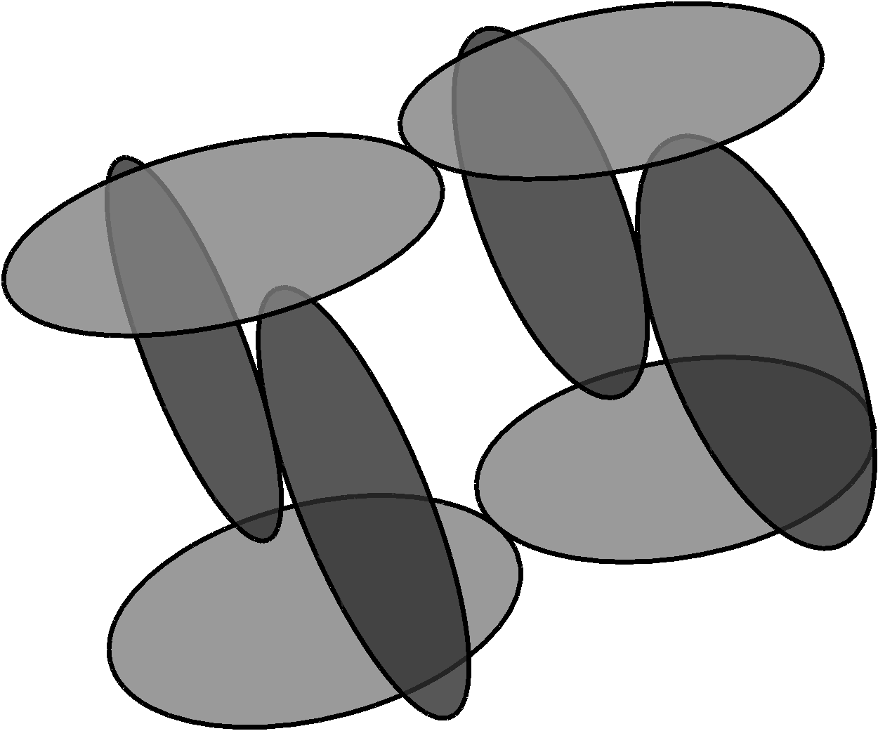
a) b)

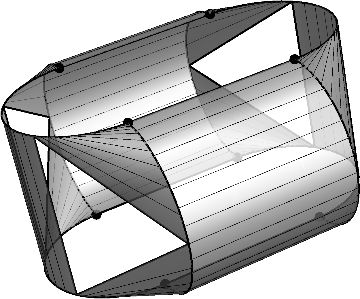
Figure 1. a) Unit disks with normal vectors in $z$-direction centered at $(0,\pm 1,\pm 1)$ (respectively, $y$-direction at $(\pm 1,\pm 1,0)$). b) The convex hull of the eight disks from a) is sketched, only the boundary is depicted, two-dimensional faces are deleted, ruled surfaces are striped, and non-exposed points are marked at $(\pm 1,\pm 1,\pm 1)$.

Example 5.9 (Polar of four stadia, $\mathcal{C}_{3}^{\prime}\subsetneq\mathcal{C}_{3}^{\prime*}$).

Analogous to Theorem 5.4(3) one proves that $K\in\mathcal{C}_{m}^{\prime*}$ holds if and only if every exposed point of every proper exposed face of $K^{\circ}$ lies in $\mathcal{E}_{K^{\circ}}$. Therefore, if $L$ is a convex body with a non-exposed point, every exposed point of whose proper exposed faces is an exposed point of $L$ then the polar $K^{\circ}=L$ satisfies $K\in\mathcal{C}_{3}^{\prime*}\setminus\mathcal{C}_{3}^{\prime}$.

Let $L$ be the convex set defined in Figure 1, which is the convex hull of a cube with four half-cylinders attached, or the convex hull of four stadia. Two of the stadia lie in $\mathcal{E}_{L}$ and include eight non-exposed points of $L$. Their four straight sides are non-exposed faces of $L$. Therefore the eight non-exposed points of $L$ are no exposed points of any proper exposed face of $L$. This completes the example.

It has nothing to do with the inclusion $\mathcal{C}_{3}^{\prime}\subsetneq\mathcal{C}_{3}^{\prime*}$, but is nevertheless interesting that $L$ is the convex support (6.4) of three $16$-by-$16$ matrices and therefore the results of the Sections 3 and 4 apply to $L$. Indeed, the unit disk with normal vector in $z$-direction centered at $(0,1,1)$ is the convex support of

$$F_{1}=\left(\begin{smallmatrix}0&1\\ 1&0\end{smallmatrix}\right),\qquad F_{2}=\left(\begin{smallmatrix}1&-\operatorname{i}\\ \operatorname{i}&1\end{smallmatrix}\right),\qquad F_{3}=\left(\begin{smallmatrix}1&0\\ 0&1\end{smallmatrix}\right).$$

Similarly the other seven disks of Figure 1a) are convex support sets and their convex hull $L$ is the convex support of the direct sum of those matrices.

The lattice of exposed faces $\mathcal{E}_{L}$ has six coatoms of dimension two (two stadia and four triangles). The reminder of the boundary of $L$ is covered by four cylindrical and eight curved ruled surfaces. The straight segments on the curved ruled surface of the positive octant have end-points $(\cos(\varphi),1+\sin(\varphi),1)$ and $(1+\sin(\psi),1,\cos(\psi))$, where

$$\cos(\psi)=\tfrac{2\cos(\varphi)-1}{2-2\cos(\varphi)+\cos(2\varphi)},\qquad\sin(\psi)=\tfrac{4\cos(\varphi)\sin(\tfrac{\varphi}{2})^{2}}{2-2\cos(\varphi)+\cos(2\varphi)},\qquad\varphi\in(0,\tfrac{\pi}{3}).$$

All boundary points of $L$ are smooth except for the exposed points. They cover a half-circle of each of the eight disks used to define $L$ in Figure 1. Having a two-dimensional normal cone, each of them is the intersection of a unique pair of coatoms of $\mathcal{E}_{L}$ (segment, triangle, or stadium) by Corollary 4.2(2).

Example 5.10 (Polar of truncated torus, $\mathcal{C}_{3}^{\prime*}\subsetneq\mathcal{C}_{3}$).

Consider the convex hull $K$ of the torus $\{(x,y,z)\in\mathbb{R}^{3}\mid p(x,y,z)=0\}$ defined by

$$p:=(x^{2}+y^{2}+z^{2})^{2}-4(x^{2}+y^{2})$$

which is a torus with rotation symmetry about the $z$-axis and self-intersection at the origin $0\in\mathbb{R}^{3}$. The radius from $0$ to the center of the torus tube and the radius of the tube are both equal one. The convex body $K$ is smooth, so $K\in\mathcal{C}_{3}^{\prime\prime}$, and has the following proper exposed faces:

$$D_{\pm}:=\{(x,y,\pm 1)\in\mathbb{R}^{3}\mid x^{2}+y^{2}\leq 1\}\qquad\mbox{(two disks)}$$

and exposed points $(x,y,z)$ for $x,y,z\in\mathbb{R}$ such that $p(x,y,z)=0$ and $x^{2}+y^{2}>1$. The non-exposed points of $K$ are

$$\xi_{\pm}(\varphi):=(\cos(\varphi),\sin(\varphi),\pm 1),\quad\varphi\in[0,2\pi).$$

By intersecting $K$ with three half-spaces ($\varphi_{0}=0,\varphi_{1}=\tfrac{2}{3}\pi,\varphi_{2}=\tfrac{4}{3}\pi$) we define

$$L:=\{(x,y,z)\in K\mid x\cos(\varphi_{i})+y\sin(\varphi_{i})\leq 1,i=0,1,2\}.$$

The convex body $L$ has five 2D exposed faces, namely $D_{\pm}$ and the exposed faces in the boundaries of the three half-spaces. The latter three exposed faces of $L$ contain no non-exposed points of $L$. The disk $D_{\pm}$ contains three exposed points $\xi_{\pm}(\varphi_{1})$, $\xi_{\pm}(\varphi_{2})$, $\xi_{\pm}(\varphi_{3})$ of $L$ while the remaining exposed points of $D_{\pm}$ are non-exposed points of $L$. The convex body $L$ has no 1D exposed faces. This discussion of exposed points of $L$ and Theorem 5.4(2),(3) show $L^{\circ}\in\mathcal{C}_{3}\setminus\mathcal{C}_{3}^{\prime}$.

6. State spaces of operator systems

Theorem 6.2 proves that the state space $\mathcal{M}(S)$ of an operator system $S$ of $M_{n}$ is the projection of the state space $\mathcal{M}_{n}$ of the matrix algebra $M_{n}$ onto the real space $S{}_{\rm h}\subset S$ of hermitian matrices. We point out that

• $\mathcal{M}(S)\in\mathcal{C}_{m}^{\prime\prime}$ for $m=\dim_{\mathbb{C}}(S)-1$ (remove one codimension of $\mathcal{M}(S)$ from $S{}_{\rm h}$),

• there is a lattice isomorphism from the ground state projections of $S{}_{\rm h}$ to the exposed faces of $\mathcal{M}(S)$,

• the ground state projections of $S{}_{\rm h}$ form a coatomistic lattice.

Some of these properties may be well-known, but we are unaware of proofs in the literature. We finish the article with representations of $\mathcal{M}(S)$ as a convex support set and convex hull of a joint numerical range and with a discussion of convex support sets of 3-by-3 matrices.

Let $S\subset M_{n}$ be an operator system. It is well-known that every complex linear functional $f:S\to\mathbb{C}$ has the form $f=f_{a}$ for a unique $a\in S$ where $f_{a}(s)=\langle a,s\rangle$ for all $s\in S$. Here $\langle a,b\rangle=\operatorname{tr}(a^{*}b)$ is the Hilbert-Schmidt inner product of $a,b\in S$, whose real part defines a Euclidean scalar product on $S$ where $S=S{}_{\rm h}+\operatorname{i}S{}_{\rm h}$ is an orthogonal direct sum. The functional $f_{a}$ has real values on $S{}_{\rm h}$ if and only if $a\in S{}_{\rm h}$ so the Hilbert-Schmidt inner product restricts to a Euclidean scalar product on $S{}_{\rm h}$.

Definition 6.1.

A state on an operator system $S\subset M_{n}$ is a complex linear functional $f:S\to\mathbb{C}$ which is positive, that is $f(s)\geq 0$ holds for all positive-semidefinite $s\in S$, and normalized, that is $f(\mathds{1})=1$. Let

$$\mathcal{M}(S):=\{s\in S\mid\mbox{$f_{s}$ is a state on $S$}\}.$$

In abuse of notation we call elements of $\mathcal{M}(S)$ states on $S$ and say that $\mathcal{M}(S)$ is the state space of $S$.

Let $K\subset\mathbb{R}^{m}$ be a convex body including the origin $0\in\mathbb{R}^{m}$ in its interior. The dual of $K$ is defined as the point reflection of the polar $K^{\circ}$, defined in (5.1),

$$K^{*}:=-K^{\circ}=\{u\in\mathbb{R}^{m}\mid 1+\langle u,x\rangle\geq 0,x\in K\}.$$

It follows from the properties of $K^{\circ}$ that $K^{*}$ is a convex body with the origin in its interior and that $(K^{*})^{*}=K$ holds. Similarly, the dual of a convex cone $K\subset\mathbb{R}^{m}$ is

$$K^{*}=\{u\in\mathbb{R}^{m}\mid\langle u,x\rangle\geq 0,x\in K\}$$

and $K$ is self-dual, if $K=K^{*}$ holds. For every real subspace $X\subset(M_{n}){}_{\rm h}$ the mapping $\pi_{X}:(M_{n}){}_{\rm h}\to X$ denotes the orthogonal projection from $(M_{n}){}_{\rm h}$ onto $X$.

The following proof uses a property of self-dual convex cones: Projections of certain cone bases are dual to bounded affine sections through their interior.

Theorem 6.2.

If $S\subset M_{n}$ is an operator system then $\mathcal{M}(S)=\pi_{S{}_{\rm h}}(\mathcal{M}_{n})$.

Proof: It is well-known, see for instance [8], that the cone $K$ of positive semi-definite matrices of $M_{n}$ is self-dual with respect to $(M_{n}){}_{\rm h}$. Without loss of generality, let $\dim_{\mathbb{C}}(S)>1$. Then the space $S_{0}\subset S{}_{\rm h}$ of traceless hermitian matrices of $S$ has dimension $\dim_{\mathbb{R}}(S_{0})=\dim_{\mathbb{C}}(S)-1>0$. The affine section

$$\mathbb{A}:=K\cap(\tfrac{1}{n}\mathds{1}+S_{0})=\mathcal{M}_{n}\cap(\tfrac{1}{n}\mathds{1}+S_{0})$$

of $K$ is bounded and contains the trace state $\tfrac{1}{n}\mathds{1}$, which is an interior point with respect to $(M_{n}){}_{\rm h}$ of $K$. Since $\mathcal{M}_{n}=(\tfrac{1}{n}\mathds{1}+\mathds{1}^{\perp})\cap K$ holds, where $\mathds{1}^{\perp}$ denotes orthogonal complement, Theorem 2.16 of [42] proves (duals with respect to $S_{0}$)

1. $\mathbb{A}-\tfrac{1}{n}\mathds{1}=\tfrac{1}{n}\pi_{S_{0}}(\mathcal{M}_{n})^{*}$

2. $\pi_{S_{0}}(\mathcal{M}_{n})=\tfrac{1}{n}(\mathbb{A}-\tfrac{1}{n}\mathds{1})^{*}$.

On the other hand, an easy computation shows

$$\mathcal{M}(S) =\{s\in S{}_{\rm h}\mid\langle s,\mathds{1}\rangle=1,\langle s,a\rangle\geq 0\,\forall a\in\mathbb{A}\}$$

$$=\tfrac{1}{n}\mathds{1}+\{s_{0}\in S_{0}\mid\langle\tfrac{1}{n}\mathds{1}+s_{0},a\rangle\geq 0\,\forall a\in\mathbb{A}\}$$

$$=\tfrac{1}{n}\mathds{1}+\{s_{0}\in S_{0}\mid\tfrac{1}{n}+\langle s_{0},a_{0}\rangle\geq 0\,\forall a_{0}\in\mathbb{A}-\tfrac{1}{n}\mathds{1}\},$$

that is

1. $\mathcal{M}(S)=\tfrac{1}{n}(\mathds{1}+(\mathbb{A}-\tfrac{1}{n}\mathds{1})^{*})$.

Substituting ii) into iii) gives $\mathcal{M}(S)=\tfrac{1}{n}\mathds{1}+\pi_{S_{0}}(\mathcal{M}_{n})$ which proves the claim. $\square$

State spaces lie in $\mathcal{C}_{m}^{\prime\prime}$. More precisely the following holds, if we identify the space of traceless hermitian matrices of a $d$-dimensional operator system with $\mathbb{R}^{d-1}$.

Corollary 6.3.

If $S\subset M_{n}$ is an operator system of dimension $d:=\dim_{\mathbb{C}}(S)>1$ then $\mathcal{M}(S)-\tfrac{1}{n}\mathds{1}\in\mathcal{C}_{d-1}^{\prime\prime}$.

Proof: One can see from the proof of Theorem 6.2 that zero is an interior point with respect to $S_{0}$ of $\mathcal{M}(S)-\tfrac{1}{n}\mathds{1}=\pi_{S_{0}}(\mathcal{M}_{n})$. Further i) of Theorem 6.2 shows that the polar of $\pi_{S_{0}}(\mathcal{M}_{n})$ is an affine section of $\mathcal{M}_{n}$. Since $\mathcal{M}_{n}$ has no non-exposed faces [33, 1] it follows that this affine section has no non-exposed faces either. Then Theorem 5.4(4) proves the claim. $\square$

Analogues of Corollary 6.3 were proved in Fact 3.2 of [40] for convex support sets, defined below. One of the proofs uses that $\mathcal{M}_{n}-\tfrac{1}{n}\mathds{1}$ lies in $\mathcal{C}_{n^{2}-1}^{\prime\prime}$ so the projection $\pi_{S_{0}}(\mathcal{M}_{n})$ lies in $\mathcal{C}_{d-1}^{\prime\prime}$ by Remark 5.3.

We provide details about the lattice isomorphism from ground state projections of hermitian operators of an operator system to the exposed faces of the state space.

Remark 6.4.

Let us begin with the full operator system $S=M_{n}$ where the isomorphism is well-known, see Section 6 of [4], Chapter 3 of [1], and the references therein. We denote the set of projections $p=p^{*}=p^{2}\in M_{n}$ by $\mathcal{P}$. Endowed with the partial ordering on $(M_{n}){}_{\rm h}$ defined by

(6.1) $$a\preceq b\quad\iff\quad b\succeq a\quad\iff\quad\mbox{$b-a$ is positive semi-definite}$$

the set $\mathcal{P}$ is a complete lattice. One can represent $\mathcal{P}$ in terms of the images of the projections, ordered by inclusion, see for example Chapter 2 of [1]. The infimum in this lattice of subspaces is the intersection. Let $u\in(M_{n}){}_{\rm h}$ be a hermitian matrix and

$$u=\sum_{\lambda}\lambda p_{u,\lambda},\quad\mathds{1}=\sum_{\lambda}p_{u,\lambda},\quad p_{u,\lambda}=p_{u,\lambda}^{*}=p_{u,\lambda}^{2}\in M_{n}$$

its spectral decomposition ($\lambda$ extends over the eigenvalues of $u$). The ground state projection of $u$ is the spectral projection $p_{-}(u):=\min_{\lambda}p_{u,\lambda_{-}(u)}$ of the least eigenvalue $\lambda_{-}(u)$ of $u$. The exposed face of $\mathcal{M}_{n}$ with inward pointing normal vector $u\in(M_{n}){}_{\rm h}$

$$F_{\mathcal{M}_{n}}(u):=\operatorname*{argmin}\{\langle\rho,u\rangle\mid\rho\in\mathcal{M}_{n}\}$$

is well-known to be expressible in the form

$$F_{\mathcal{M}_{n}}(u)=\{\rho\in\mathcal{M}_{n}\mid{\rm Image}(\rho)\subset{\rm Image}(p_{-}(u))\}$$

in terms of the ground state projection of $u$, and $\mathcal{P}\to\mathcal{E}_{\mathcal{M}_{n}}$, $p\mapsto F_{\mathcal{M}_{n}}(-p)$, is a lattice isomorphism to the exposed faces of $\mathcal{M}_{n}$.

Consider now the state space $\mathcal{M}(S)$ of an operator system $S\subset M_{n}$. It is easy to see that for $s\in S{}_{\rm h}$ the exposed face

$$F_{\mathcal{M}(S)}(s):=\operatorname*{argmin}\{\langle\rho,s\rangle\mid\rho\in\mathcal{M}(S)\}$$

lifts to the corresponding exposed face of $\mathcal{M}_{n}$, that is $F_{\mathcal{M}_{n}}(s)=\pi_{S{}_{\rm h}}|_{\mathcal{M}_{n}}^{-1}(F_{\mathcal{M}(S)}(s))$. Indeed, the map

(6.2) $$\mathcal{E}_{\mathcal{M}(S)}\to\mathcal{E}_{\mathcal{M}(S)}^{\prime}:=\{\pi_{S{}_{\rm h}}|_{\mathcal{M}_{n}}^{-1}(F)\mid F\in\mathcal{E}_{\mathcal{M}(S)}\}$$

is a lattice isomorphism whose range $\mathcal{E}_{\mathcal{M}(S)}^{\prime}$ is ordered by inclusion. Moreover, the infimum of $\mathcal{E}_{\mathcal{M}(S)}^{\prime}$ is just the restriction of the infimum of $\mathcal{E}_{\mathcal{M}_{n}}$ to $\mathcal{E}_{\mathcal{M}(S)}^{\prime}$, which is the intersection (see Proposition 5.6 of [43]). Let

$$\mathcal{P}(S):=\{p_{-}(s)\mid s\in S{}_{\rm h}\}\cup\{0\}$$

denote the set of ground state projections of $S{}_{\rm h}$ endowed with the partial ordering (6.1). Notice that $p_{-}(s)$ may not lie in $S$ for some $s\in S{}_{\rm h}$. Since (6.2) is a lattice isomorphism, the lattice isomorphism $\mathcal{P}\to\mathcal{E}_{\mathcal{M}_{n}}$ restricts to a lattice isomorphism $\mathcal{P}(S)\to\mathcal{E}_{\mathcal{M}(S)}^{\prime}$ and combines with (6.2) to a lattice isomorphism

(6.3) $$\mathcal{P}(S)\to\mathcal{E}_{\mathcal{M}(S)},\quad p\mapsto\pi_{S_{h}}(F_{\mathcal{M}_{n}}(-p)).$$

The isomorphism (6.3) is described in Section 3.1 of [42]. We stress that the infimum of $\mathcal{P}(S)$ is the restriction of the infimum of $\mathcal{P}$ because the the infimum of $\mathcal{E}_{\mathcal{M}(S)}^{\prime}$ is the restriction of the infimum of $\mathcal{E}_{\mathcal{M}_{n}}$.

If projections are represented in terms of their images then the infimum of $\mathcal{E}_{\mathcal{M}(S)}$ and of $\mathcal{P}(S)$ are both given by the intersection. This is especially nice in the following corollary.

Corollary 6.5.

If $S\subset M_{n}$ is an operator system then the lattice of ground state projections $\mathcal{P}(S)$ is coatomistic.

Proof: This follows from Corollary 6.3, Lemma 4.4, and Corollary 4.5(1). $\square$

We now recall two coordinate representations of state spaces (and show that polytopes belong to them). We define the convex support of $F_{i}\in(M_{n}){}_{\rm h}$, $i=1,\ldots,k$, $k\in\mathbb{N}$, by

(6.4) $$\operatorname{cs}(F_{1},\ldots,F_{k}):=\{\langle\rho,F_{i}\rangle_{i=1}^{k}\mid\rho\in\mathcal{M}_{n}\}$$

and the joint numerical range (using the inner product of $\mathbb{C}^{n}$) by

$$W(F_{1},\ldots,F_{k}):=\{\langle x,F_{i}(x)\rangle_{i=1}^{k}\mid\langle x,x\rangle=1,x\in\mathbb{C}^{n}\}.$$

Remark 6.6 (Convex support sets).

1. State spaces and convex support sets. Let $S\subset M_{n}$ be an operator system and let $F_{i}\in(M_{n}){}_{\rm h}$ for $i=1,\ldots,k$, such that $\{\mathds{1},F_{1},\ldots,F_{k}\}$ spans $S{}_{\rm h}$. Then it is easy to see that the linear map

   $$\alpha:S{}_{\rm h}\to\mathbb{R}^{k+1},s\mapsto(\langle s,\mathds{1}\rangle,\langle s,F_{1}\rangle,\ldots,\langle s,F_{k}\rangle)$$

   restricts to a bijection $S{}_{\rm h}\to\alpha(S{}_{\rm h})$. Hence $\mathcal{M}(S)\cong\operatorname{cs}(\mathds{1},F_{1},\ldots,F_{k})$ and $\mathcal{M}(S)\cong\operatorname{cs}(F_{1},\ldots,F_{k})$ are isomorphic, see Remark 1.1(1) of [42] for a proof.

2. Convex support sets and joint numerical ranges. If $F_{i}\in(M_{n}){}_{\rm h}$, $i=1,\ldots,k$, then

   $$\operatorname{cs}(F_{1},\ldots,F_{k})=\operatorname{conv}\left(W(F_{1},\ldots,F_{k})\right).$$

   For a proof see [29] or Section 2 of [40]. For $k=2$ the joint numerical range $W(F_{1},F_{2})$ is the numerical range of $F_{1}+\operatorname{i}F_{2}$ which is convex for all $n\in\mathbb{N}$ by the Toeplitz-Hausdorff theorem. The joint numerical range is convex for $k=3$ and $n\geq 3$, but fails to be convex in general for $k\geq 4$ [3, 26, 18].

3. Polytopes. Consider a collection of $n$ points $p_{j}\in\mathbb{R}^{m}$, $n,m\in\mathbb{N}$. Define an $m$-by-$n$-matrix $M$ whose $j$’s column is $p_{j}$, $j=1,\ldots,n$, and define diagonal matrices $F_{i}\in M_{n}$ where $\operatorname{diag}(F_{i})$ is the $i$’s row of $M$, $i=1,\ldots,m$. Then the convex support $\operatorname{cs}(F_{1},\ldots,F_{m})$ is the convex hull of $\{p_{1},\ldots,p_{n}\}\subset\mathbb{R}^{m}$.

We discuss convex support sets of $3$-by-$3$ matrices.

Example 6.7.

Consider the convex support $\operatorname{cs}(F)$ of $k\in\mathbb{N}$ hermitian $3$-by-$3$ matrices $F=(F_{1},\ldots,F_{k})$ and assume without loss of generality that $\operatorname{cs}(F)$ has an interior point. Then $\operatorname{cs}(F)\in\mathcal{C}_{k}^{\prime\prime}$ holds by Remark 6.6(1) and Corollary 6.3.

The subset of non-smooth points $\partial_{\rm n}\operatorname{cs}(F)$ of the boundary $\partial\operatorname{cs}(F)$ consists of the non-smooth exposed points. Indeed, The form of a proper exposed face $G$ of $\operatorname{cs}(F)$ is very restricted for $3$-by-$3$ matrices. It may be a singleton (exposed point), either smooth or not. Otherwise $G$ is a segment, a filled ellipse, or filled ellipsoid [40]. We see that proper exposed faces of $\operatorname{cs}(F)$ have no segments on their relative boundary. Therefore, if $G$ is not a singleton then it is necessarily a coatom of $\mathcal{E}_{\operatorname{cs}(F)}$ and is therefore smooth (has a unique unit normal vector) by Theorem 3.2. For the same reason, every non-exposed face of $\operatorname{cs}(F)$ is a singleton. Moreover, every non-exposed point is smooth because it has the same normal cone as the smallest exposed face in which it is contained (see Lemma 4.6 of [43]). This proves the claim. Equivalently, $\partial_{\rm n}\operatorname{cs}(F)$ is the set of intersection points of pairs of mutually distinct coatoms of $\mathcal{E}_{\operatorname{cs}(F)}$ by Corollary 2.3.

A notable property of $3$-by-$3$ matrices is that each two coatoms of $\mathcal{E}_{\operatorname{cs}(F)}$ which are both no singletons must intersect. This follows from the analogue property of $k=2$ by projecting $\operatorname{cs}(F)$ onto the span of the normal vectors of these coatoms (for a proof when $k=3$ see Lemma 5.1 of [40], $k>3$ is analogous). The case $k=2$ is solved by the classification of the numerical range of $3$-by-$3$ matrices [24, 23]. So, $\mathcal{E}_{\operatorname{cs}(F)}$ has only one cluster of coatoms of positive dimension, in the sense of Corollary 2.4.

The classification [40] proves that $\partial_{\rm n}\operatorname{cs}(F)$ is closed for $k=3$. If $\operatorname{cs}(F)$ has a corner then $\operatorname{cs}(F)$ is either the convex hull of an ellipsoid and a point outside the ellipsoid or the convex hull of an ellipse and a point outside the affine hull of the ellipse. In the first case $\partial_{\rm n}\operatorname{cs}(F)$ is a singleton, in the second case $\partial_{\rm n}\operatorname{cs}(F)$ is the union of an ellipse and a singleton. If $\operatorname{cs}(F)$ has no corner then the cluster of $\mathcal{E}_{\operatorname{cs}(F)}$ with coatoms of positive dimension contains $s$ segments and $e$ ellipses such that

$$(s,e)\in\{\begin{smallmatrix}(0,0)\end{smallmatrix},\begin{smallmatrix}(0,1)\end{smallmatrix},\begin{smallmatrix}(0,2)\end{smallmatrix},\begin{smallmatrix}(0,3)\end{smallmatrix},\begin{smallmatrix}(0,4)\end{smallmatrix},\begin{smallmatrix}(1,0)\end{smallmatrix},\begin{smallmatrix}(1,1)\end{smallmatrix},\begin{smallmatrix}(1,2)\end{smallmatrix}\}.$$

The coatoms of this cluster intersect in pairs but not in triples so $\partial_{\rm n}\operatorname{cs}(F)$ has cardinality ${s+e\choose 2}\in\{0,1,3,6\}$. Since $\partial_{\rm n}\operatorname{cs}(F)$ is closed it follows that its complement $\partial\operatorname{cs}(F)\setminus\partial_{\rm n}\operatorname{cs}(F)$ is a $C^{1}$-submanifold of $\mathbb{R}^{3}$ (Theorem 2.2.4 of [38] can be used locally to prove this).

Acknowledgements. The author thanks Eduardo Garibaldi, Fernando Torres, and especially Marcelo Terra Cunha for discussions. He is grateful for Arleta Szkoła’s comments on an earlier manuscript. This work is supported by a PNPD/CAPES scholarship of the Brazilian Ministry of Education.

References

- [1] E. M. Alfsen and F. W. Shultz (2001) State Spaces of Operator Algebras: Basic Theory, Orientations, and C*-Products, Boston: Birkhäuser
- [2] L. Arrachea, N. Canosa, A. Plastino, M. Portesi, and R. Rossignoli (1992) Maximum-entropy approach to critical phenomena in ground states of finite systems, Phys Rev A 45 7104–7110
- [3] Y. H. Au-Yeung and Y. T. Poon (1979) A remark on the convexity and positive definiteness concerning Hermitian matrices, Southeast Asian Bull Math 3 85–92
- [4] G. P. Barker and D. Carlson (1975) Cones of diagonally dominant matrices, Pac J Math 57 15–32
- [5] G. P. Barker (1978) Faces and duality in convex cones, Linear Multilinear A 6 161–169
- [6] O. Barndorff-Nielsen (1978) Information and Exponential Families in Statistical Theory, Chichester: John Wiley & Sons Ltd
- [7] I. Bengtsson and K. Życzkowski (2006) Geometry of Quantum States, Cambridge: Cambridge University Press
- [8] A. Berman and A. Ben-Israel (1973) Linear equations over cones with interior: A solvability theorem with applications to matrix theory, Linear Algebra Appl 7 139–149
- [9] G. Birkhoff (1967) Lattice Theory, 3rd ed., Providence, R.I.: AMS
- [10] J. Chen, Z. Ji, D. Kribs, Z. Wei, and B. Zeng (2012) Ground-state spaces of frustration-free Hamiltonians, J Math Phys 53 102201
- [11] J. Chen, Z. Ji, C.-K. Li, Y.-T. Poon, Y. Shen, N. Yu, B. Zeng, and D. Zhou (2015) Discontinuity of maximum entropy inference and quantum phase transitions, New J Phys 17 083019
- [12] J. Chen, Z. Ji, M. B. Ruskai, B. Zeng, and D.-L. Zhou (2012) Comment on some results of Erdahl and the convex structure of reduced density matrices, J Math Phys 53 072203
- [13] J. Chen, Z. Ji, B. Zeng, and D. L. Zhou (2012) From ground states to local Hamiltonians, Phys Rev A 86 022339
- [14] W.-S. Cheung, X. Liu, and T.-Y. Tam (2011) Multiplicities, boundary points, and joint numerical ranges, Oper Matrices 1 41–52
- [15] M.-T. Chien and H. Nakazato (2010) Joint numerical range and its generating hypersurface, Linear Algebra Appl 432 173–179
- [16] R. M. Erdahl (1972) The convex structure of the set of N-representable reduced 2-matrices, J Math Phys 13 1608–1621
- [17] B. Grünbaum (2003) Convex Polytopes, 2nd ed., New York: Springer
- [18] E. Gutkin, E. A. Jonckheere, and M. Karow (2004) Convexity of the joint numerical range: topological and differential geometric viewpoints, Linear Algebra Appl 376 143–171
- [19] E. Gutkin and K. Życzkowski (2013) Joint numerical ranges, quantum maps, and joint numerical shadows, Linear Algebra Appl 438 2394–2404
- [20] T. Heinosaari, L. Mazzarella, and M. M. Wolf (2013) Quantum tomography under prior information, Commun Math Phys 318 355–374
- [21] A. Holevo (2011) Probabilistic and Statistical Aspects of Quantum Theory, 2nd edition, Pisa: Edizioni della Normale
- [22] E. Jaynes (1957) Information theory and statistical mechanics. II, Phys Rev 108 171–190
- [23] D. S. Keeler, L. Rodman, and I. M. Spitkovsky (1997) The numerical range of matrices, Lin Alg Appl 252 115–139
- [24] R. Kippenhahn (1951) Über den Wertevorrat einer Matrix, Math Nachr 6 193–228
- [25] N. Krupnik and I. M. Spitkovsky (2006) Sets of matrices with given joint numerical range, Linear Algebra Appl 419 569–585
- [26] C.-K. Li and Y.-T. Poon (2000) Convexity of the joint numerical range, SIAM J Matrix Anal A 21 668–678
- [27] R. Loewy and B.-S. Tam (1986) Complementation in the face lattice of a proper cone, Linear Algebra Appl 79 195–207
- [28] V. Magron, D. Henrion, and J.-B. Lasserre (2015) Semidefinite approximations of projections and polynomial images of semialgebraic sets, SIAM J Optimiz 25 2143–2164
- [29] V. Müller (2010) The joint essential numerical range, compact perturbations, and the Olsen problem, Stud Math 197 275–290
- [30] T. Netzer, D. Plaumann, and M. Schweighofer (2010) Exposed faces of semidefinitely representable sets, SIAM J Optimiz 20 1944–1955
- [31] S. A. Ocko, X. Chen, B. Zeng, B. Yoshida, Z. Ji, M. B. Ruskai, and I. L. Chuang (2011) Quantum codes give counterexamples to the unique preimage conjecture of the N-representability problem, Phys Rev Lett 106 110501
- [32] V. I. Paulsen (2002) Completely Bounded Maps and Operator Algebras, New York: Cambridge University Press
- [33] M. Ramana and A. J. Goldman (1995) Some geometric results in semidefinite programming, J Global Optim 7 33–50
- [34] R. T. Rockafellar (1970) Convex Analysis, Princeton: Princeton University Press
- [35] L. Rodman, I. M. Spitkovsky, A. Szkoła, and S. Weis (2016) Continuity of the maximum-entropy inference: Convex geometry and numerical ranges approach, J Math Phys 57 015204
- [36] P. Rostalski and B. Sturmfels (2013) Dualities, 203–249 of G. Blekherman, P. Parrilo, and R. Thomas, Eds., Semidefinite Optimization and Convex Algebraic Geometry, MOS-SIAM series on optimization, Philadelphia: SIAM
- [37] R. Sanyal, F. Sottile, and B. Sturmfels (2011) Orbitopes, Mathematika 57 275–314
- [38] R. Schneider (2014) Convex bodies: The Brunn-Minkowski theory, 2nd ed., New York: Cambridge University Press
- [39] R. Sinn and B. Sturmfels (2015) Generic spectrahedral shadows, SIAM J Optimiz 25 1209–1220
- [40] K. Szymański, S. Weis, and K. Życzkowski (submitted) Classification of joint numerical ranges of three hermitian matrices of size three, arXiv:1603.06569 [math.FA]
- [41] B.-S. Tam (1985) On the duality operator of a convex cone, Lin Alg Appl 64 33–56
- [42] S. Weis (2011) Quantum convex support, Linear Algebra Appl 435 3168–3188
- [43] S. Weis (2012) A note on touching cones and faces, J Convex Anal 19 323–353
- [44] S. Weis (2012) Duality of non-exposed faces, J Convex Anal 19 815–835
- [45] S. Weis and A. Knauf (2012) Entropy distance: New quantum phenomena, J Math Phys 53 102206
- [46] S. Weis (2014) Continuity of the maximum-entropy inference, Commun Math Phys 330 1263–1292
- [47] G. M. Ziegler (1995) Lectures on Polytopes, New York: Springer-Verlag
Stephan Weis
e-mail: maths@stephan-weis.info
Departamento de Matem tica
Instituto de Matem tica, Estat stica e Computa o Cient fica
Universidade Estadual de Campinas
Rua S rgio Buarque de Holanda, 651
Campinas-SP, CEP 13083-859
Brazil
Centre for Quantum Information and Communication
Ecole Polytechnique de Bruxelles
Universit Libre de Bruxelles
50 av. F.D. Roosevelt - CP165/59
B-1050 Bruxelles
Belgium