$SO(10)$ thick branes and perturbative stability

Abstract

Three self-gravitating $SO(10)$ domain walls in five dimensions are obtained and their properties are analyzed. These non-abelian domain walls interpolate between AdS₅ spacetimes with different embedding of $SU(5)$ in $SO(10)$ and they can be distinguished, among other features, by the unbroken group on each wall, being either $SO(10)$, $SO(6)\otimes SU(2)\otimes U(1)/Z_{2}$ or $SU(4)\otimes SO(2)\otimes U(1)/Z_{4}$. We show that, unlike Minkowskian versions, the curved scenarios are perturbatively stable due to the gravitational capture of scalar fluctuations associated to the residual orthogonal subgroup in the core of the walls. These stabilizer modes are additional to the four-dimensional Nambu-Goldstone states found in two of the three gravitational sceanarios.

I Introduction

Our universe could be a hypersurface embedded in a higher dimensional spacetime and among the proposals that have emerged to develop this idea, the five-dimensional Randall-Sundrum model Randall:1999vf has received much attention because standard gravitation can be recovered on the four-dimensional worldsheet (or 3-brane) of the scenario. For a discussion about localization of matter and interaction fields, see Bajc:1999mh ; Dvali:2000rx .

In more realistic models the thickness of the worldsheet is taken into account, in this case the brane is generated by a domain wall, a solution to Einstein gravity theory interacting with a scalar field where the scalar field is a standard kink interpolating between the minima of a potential with spontaneously broken symmetry Gremm:1999pj ; DeWolfe:1999cp ; Wang:2002pka ; Bazeia:2003aw ; Melfo:2002wd ; CastilloFelisola:2004eg ; Melfo:2006hh ; Guerrero:2006gj ; Guerrero:2009ac . This scenarios are topologically stables and, consequently, the analysis of small fluctuations of both the metric tensor and the scalar field Giovannini:2001fh , revels a tower of modes free of tachyonic instabilities.

Domain walls generated from several scalar fields have been also considered, see Ref. George:2011tn , and among other properties, it is observed that the flat configuration admits the translation zero mode in Kaluza-Klein spectrum of the scalar perturbations which is removed when the extra dimension is warped; however, the general set-up, in the presence of gravity, can support one or several extra zero modes in the excitations tower.

It is also possible to consider domain walls with multiple scalar fields in terms of a non-abelian source with internal gauge symmetry group $G$, which is advantageous on the wall, where our universe is realized, because a symmetry breaking pattern, $G\rightarrow H_{0}$, could be obtained. This opens up the possibility of building braneworld with Standard Model group on the wall. In this sense several attempts have been made; in particular, a pair of perturbatively stable self-gravitating $SU(5)\otimes Z_{2}$ domain walls, with different group $H_{0}$, were reported in Melfo:2011ev . Remarkably, one of them corresponds to curved version of the flat solution found in Pogosian:2000xv and widely disscused in Vachaspati:2001pw ; Pogosian:2001pq ; Vachaspati:2003zp . Other notable attempt, with $G=E_{6}$ but in flat space, was reported in Davidson:2007cf .

The perturbative stability analysis of the $SU(5)\otimes Z_{2}$ walls was performed in Pantoja:2015yin (as far as we know, there is no a topologiacal charge difined for non-abelian walls) and, in addition to verifying the local stability of scenarios, it was shown that, for a four-dimensional observer localized on the brane, the tensor and vector sectors of the gravity fluctuations behave in a similar way to the abelian domain wall set-up Giovannini:2001fh ; namely, while the zero mode of the tensor excitations is localized, there is not a nomalizable solution for the vector perturbations. On the other hand, in the spectrum of the scalar fluctuations, the absence of the translation mode was verified and normalizable massless scalar modes associated to the particular symmetry breaking pattern considered on the wall were found.

From the point of view of Grand Unified Theories, the symmetry $O(10)$ is considered more fundamental that $U(5)$ in the sense that $SU(5)\subset SO(10)$ and the Standard Model group is embedded in $SO(10)$ as a single irreducible representation of the underlying gauge group. In Shin:2003xy , three flat $SO(10)$ domain walls were found and, just as in $SU(5)\otimes Z_{2}$ case, a symmetry breaking pattern, $SO(10)\rightarrow H_{0}$, was determined for each wall. These scenarios will be considered in this paper; concretely, we will focus on both the extension to curved spacetime and the stability under small perturbations. Among the results that we will show highlight, the local instability of two of the flat scenarios due to tachyonic Pöschl-Teller modes in spectrum of scalar perturbations, which, fortunately, can be removed when gravity is included; and, the four-dimensional localization of massless scalar states along the broken generators associated to $SO(10)\rightarrow H_{0}$, which occurs only when gravity is present in the model.

The paper is organized as follows, in Sections II and III the gravity $SO(10)$ set-up and the extensions to warped spacetime of the flat $SO(10)$ kinks are obtained. In Section IV, the perturbative stability analysis of the $SO(10)$ walls is performed and it is show that gravitation rescues the stability through the capture of massless scalar perturbations associated to the orthogonal subgroup of $H_{0}$. Finally, in Section V our results and conclusions are summarized and presented.

II Self-gravitating $SO(10)$ kinks

Consider the Einstein-scalar field coupled system in five dimensions

$$R_{ab}-\frac{1}{2}g_{ab}R=$$

$$-\frac{1}{2}\text{Tr}(\nabla_{a}\mathbf{\Phi}\nabla_{b}\mathbf{\Phi}) + g_{ab}(\frac{1}{4}\text{Tr}(\nabla_{c}\mathbf{\Phi}\nabla^{c}\mathbf{\Phi})-V(\mathbf{\Phi}))$$ (1)

and

$$\nabla_{c}\nabla^{c}\mathbf{\Phi}=\frac{\partial V(\mathbf{\Phi})}{\partial\mathbf{\Phi}},$$ (2)

where $\mathbf{\Phi}$ is a scalar multiplet in the 45-adjoint representation of $SO(10)$, i.e

$$\mathbf{\Phi}\rightarrow{\boldsymbol{O}}\mathbf{\Phi}{\boldsymbol{O}}^{\text{T}},\quad{\boldsymbol{O}}=e^{\frac{1}{2}\alpha_{j_{1}j_{2}}\mathbf{L}_{j_{1}j_{2}}}$$ (3)

with $\alpha$ and $\mathbf{L}$ the parameters and generators of the group respectively. In particular, for the generators in the fundamental representation we have

$$\left(\mathbf{L}_{j_{1}j_{2}}\right)_{j_{3}j_{4}}=\delta_{j_{1}j_{4}}\delta_{j_{2}j_{3}}-\delta_{j_{1}j_{3}}\delta_{j_{2}j_{4}}.$$ (4)

The latin index $j=1,\dots,10$, denotes an internal index of SO(10) group.

Now, consider the spacetime ($\mathbb{R}^{5}$, $\bf{g}$) where the tensor metric $\bf{g}$ for a five-dimensional static spacetime with a planar-parallel symmetry, in a particular coordinate basis, is given by

$$ds^{2}=e^{2A(y)}\eta_{\mu\nu}dx^{\mu}dx^{\nu}+dy^{2},\quad\mu,\nu=0,\dots,4.$$ (5)

We are interested in the realization of brane worlds on this geometry. In order to do this, we consider a potential of sixth-order

$$V(\mathbf{\Phi}) = V_{0}+\frac{\mu^{2}}{2}\text{Tr}\mathbf{\Phi}^{2}+\frac{h}{4}(\text{Tr}\mathbf{\Phi}^{2})^{2}+\frac{\lambda}{4}\text{Tr}\mathbf{\Phi}^{4}$$ (6)

$$+\frac{\alpha}{6}(\text{Tr}\mathbf{\Phi}^{2})^{3}+\frac{\gamma}{6}\text{Tr}\mathbf{\Phi}^{4}\text{Tr}\mathbf{\Phi}^{2}+\frac{\beta}{6}\text{Tr}\mathbf{\Phi}^{6},$$

where $V_{0}$ is a constant to be fixed.

Two aspects of the theory should be highlighted. First, the $O(10)$ group has two disconnected components, the $SO(10)$ special subgroup and the antispecial part. These two subspaces are related by a discrete $Z_{2}$ transformation of $O(10)$. Second, both $\text{Tr}(\mathbf{\Phi}^{3})$ and $\text{Tr}(\mathbf{\Phi}^{5})$ vanishes in (6) because the scalar field is antisymmetric. Therefore, the reflection symmetry

$$Z_{2}:\mathbf{\Phi}\rightarrow-\mathbf{\Phi},$$ (7)

that connects the vacuum expectation values (vev’s) of scalar field

$$\mathbf{\Phi}(y=-\infty)=-{\boldsymbol{O}}\mathbf{\Phi}(y=+\infty){\boldsymbol{O}}^{\text{T}},$$ (8)

is part of the model and is outside the $SO(10)$ group Shin:2003xy . Hence, a $SO(10)$ kink interpolating between two minima of $V(\mathbf{\Phi})$ is a feasible solution for the coupled system. A kink solution for a sixth-order polynomial potential and a single self-gravitating scalar field have been found in DeWolfe:1999cp .

We will assume that the scalar field takes values in the Cartan-subalgebra space of $SO(10)$, that is

$$\mathbf{\Phi}=\phi_{1}\mathbf{L}_{12}+\phi_{2}\mathbf{L}_{34}+\phi_{3}\mathbf{L}_{56}+\phi_{4}\mathbf{L}_{78}+\phi_{5}\mathbf{L}_{90}.$$ (9)

(Hereon we denote the subscript $10$ as $0$.) Following the usual strategy, from (II) and (2) we find

$$3A^{\prime\prime}=-\phi_{k}^{\prime}\phi_{k}^{\prime}\ ,\quad\frac{3}{2}A^{\prime\prime}+6A^{\prime 2}=-V({\bf\Phi})$$ (10)

and

$$\phi_{i}^{\prime\prime}+4A^{\prime}\phi_{i}^{\prime}=-2(\mu^{2} - 2h\phi_{k}\phi_{k})\phi_{i}+2\lambda\phi_{i}^{3}+2\beta\phi_{i}^{5}$$

$$+\frac{4\gamma}{3}(2\phi_{i}^{2}\phi_{k}\phi_{k} - \phi_{k}^{2}\phi_{k}^{2})\phi_{i}-8\alpha(\phi_{k}\phi_{k})^{2}\phi_{i},$$ (11)

where prime indicates derivative with respect to extra coordinate $y$ and $i,k=1,\dots,5$.

From the minimum of the potential we take the following three boundary conditions Li:1973mq ; Shin:2003xy

$${\mathbf{\Phi_{A}}}(y=\pm\infty)=\pm\frac{v}{\sqrt{5}}\ (\mathbf{L}_{12}+\mathbf{L}_{34}+\mathbf{L}_{56}+\mathbf{L}_{78}+\mathbf{L}_{90}),$$ (12)

$${\mathbf{\Phi_{B}}}(y=\pm\infty)=\frac{v}{\sqrt{3}}\ (\pm\mathbf{L}_{12}\pm\mathbf{L}_{34}\pm\mathbf{L}_{56}-\mathbf{L}_{78}-\mathbf{L}_{90})$$ (13)

and

$${\mathbf{\Phi_{C}}}(y=\pm\infty)=v\ (\pm\mathbf{L}_{12}-\mathbf{L}_{34}-\mathbf{L}_{56}-\mathbf{L}_{78}-\mathbf{L}_{90}).$$ (14)

Now, choosing

$$h=0,\quad\alpha=0,\quad\gamma=0,$$ (15)

in order to decouple (II), and solving the boundary value problem for

$$A=-\frac{v^{2}}{9}\left[2\ln\cosh(ky)+\frac{1}{2}\tanh^{2}(ky)\right],$$ (16)

we obtain three non-abelian kink solutions determined as follows

Symmetric kink: for the boundary condition (12), we get a kink solution with a single component,

$$\mathbf{\Phi_{A}}=v\tanh(ky)\mathbf{M_{A}},$$ (17)

such that

$$\mathbf{M_{A}}=\frac{1}{\sqrt{5}}(\mathbf{L}_{12}+\mathbf{L}_{34}+\mathbf{L}_{56}+\mathbf{L}_{78}+\mathbf{L}_{90})$$ (18)

and

$$v=\frac{\sqrt{5}}{2} \sqrt{\frac{\lambda}{\beta}-\frac{9}{10}},\quad k=\frac{3}{2\sqrt{10}}\sqrt{\beta\left(\frac{\lambda}{\beta}-\frac{9}{10}\right)},$$ (21)

$$\mu=\frac{\sqrt{3}}{4}\sqrt{\beta\left(\frac{\lambda}{\beta}+\frac{3}{10}\right)\left(\frac{\lambda}{\beta}-\frac{9}{10}\right)},$$

$$\qquad V_{0}=\frac{9}{64}\beta\left(\frac{\lambda}{\beta}-\frac{9}{10}\right)^{2},$$

with $\beta>0$ and $\lambda>9\beta/10$.

Asymmetric kink: in connection with (13), the kink solution obtained in this case has two components,

$$\mathbf{\Phi_{B}}=v\tanh(ky)\mathbf{M_{B}}-\sqrt{\frac{{2}}{3}}v\mathbf{P_{B}},$$ (22)

where

$$\mathbf{M_{B}}=\frac{1}{\sqrt{3}}(\mathbf{L}_{12}+\mathbf{L}_{34}+\mathbf{L}_{56}),\ \mathbf{P_{B}}=\frac{1}{\sqrt{2}}(\mathbf{L}_{78}+\mathbf{L}_{90})$$ (23)

and

$$v= \frac{\sqrt{3}}{2}\sqrt{\frac{\lambda}{\beta}-\frac{3}{2}},\quad k=\frac{\sqrt{3}}{2\sqrt{2}}\sqrt{\beta\left(\frac{\lambda}{\beta}-\frac{3}{2}\right)},$$ (26)

$$\mu=\frac{\sqrt{3}}{4}\sqrt{\beta\left(\frac{\lambda}{\beta}+\frac{1}{2}\right)\left(\frac{\lambda}{\beta}-\frac{3}{2}\right)},$$

$$V_{0}=\frac{1}{24}\beta\left(\frac{\lambda}{\beta}+\frac{33}{8}\right)\left(\frac{\lambda}{\beta}-\frac{3}{2}\right)^{2},$$

with $\beta>0$ and $\lambda>3\beta/2$.

Superasymmetric kink: for the condition (14), as in the previous case, we find a kink solution with components in two directions,

$$\mathbf{\Phi_{C}}=v\tanh(ky)\mathbf{M_{C}}-2v\mathbf{P_{C}},$$ (27)

where

$$\mathbf{M_{C}}=\mathbf{L}_{12},\quad\mathbf{P_{C}}=\frac{1}{2}(\mathbf{L}_{34}+\mathbf{L}_{56}+\mathbf{L}_{78}+\mathbf{L}_{90}).$$ (28)

and

$$v= \frac{1}{2}\sqrt{\frac{\lambda}{\beta}-\frac{9}{2}},\quad k=\frac{3}{2\sqrt{2}}\sqrt{\beta\left(\frac{\lambda}{\beta}-\frac{9}{2}\right)},$$ (30)

$$\mu=\frac{\sqrt{3}}{4}\sqrt{\beta\left(\frac{\lambda}{\beta}+\frac{3}{2}\right)\left(\frac{\lambda}{\beta}-\frac{9}{2}\right)},$$

$$V_{0}=\frac{1}{12}\beta\left(\frac{\lambda}{\beta}+\frac{63}{16}\right)\left(\frac{\lambda}{\beta}-\frac{9}{2}\right)^{2},$$ (31)

such that $\beta>0$ and $\lambda>9\beta/2$.

In all cases $\mathbf{M_{A,B,C}}$ and $\mathbf{P_{B,C}}$ are orthogonal generators of $SO(10)$.

The warp factor (16) together with (17), (22) or (27) represent a two-parameter family of $SO(10)$ static domain walls, asymptotically AdS₅ with cosmological constant determined by

$$\Lambda_{\bf A}=-\frac{5}{48}\beta\left(\frac{\lambda}{\beta}-\frac{9}{10}\right)^{3}$$ (32)

for the symmetric case;

$$\Lambda_{\bf B}=-\frac{1}{16}\beta\left(\frac{\lambda}{\beta}-\frac{3}{2}\right)^{3}$$ (33)

for the asymmetric case; or

$$\Lambda_{\bf C}=-\frac{1}{48}\beta\left(\frac{\lambda}{\beta}-\frac{9}{2}\right)^{3}$$ (34)

for the superasymmetric case. On the other hand, they can also be considered as the extensions to curved spacetime of the flat $SO(10)$ kinks reported in Shin:2003xy and supported on a four-order potential ( $\alpha=\gamma=\beta=0$). In this case the system is decoupled for $h=0$ and is satisfied when $k=\mu$ and $v=\sqrt{5\mu^{2}/\lambda}$, $\sqrt{3\mu^{2}/\lambda}$, $\mu/\sqrt{\lambda}$ respectively for the symmetric, asymmetric and superasymmetric kink.

III The breaking scheme of $SO(10)$ Brane

Any of the non-abelian kinks induces the breaking of $SO(10)$ both in the core and at the edge of the scenarios. The unbroken symmetry at $y\rightarrow\pm\infty$, for each kink solution, is given by

$$SO(10)\longrightarrow\frac{SU(5)\otimes U(1)}{Z_{5}},$$ (35)

and in concordance with the boundary conditions (12, 13, 14), $SU(5)$ is embedded in $SO(10)$ in different ways Li:1973mq .

In the core of the wall, the remaining groups are completely different. For the symmetric kink (17) the scalar field vanish in $y=0$; so, all generators of $SO(10)$ are annihilated for the field and the group is preserved on the wall. This is a straightforward generalization of the abelian case.

For the other scenarios the situation is more interesting. This means that some components of ${\mathbf{\Phi_{B,C}}}$ can be nonzero in the core, and some generators of $SO(10)$ remain broken even in the core. Therefore, the spontaneous symmetry breaking is non-trivially realized on the wall. To see this explicitly we consider a combinations $\mathbf{T}$ of generators $\mathbf{L}$ such that $\partial^{2}V({\mathbf{\Phi}})/\partial\phi_{j_{1}}\partial\phi_{j_{2}}$ is diagonal for each kink solution $\mathbf{\Phi_{B,C}}$. For the asymmetric kink we find that $SO(3)$ sector of $SO(10)$ is isomorphically equivalent to $SU(2)$; on the other hand, for the superasymmetric kink, we get that $SO(6)$ sector of $SO(10)$ becomes isomorphic to $SU(4)$.

Therefore, in the core of the non-abelian walls (22) and (27) respectively we have

$$SO(10)\longrightarrow H_{\mathbf{B}}=\frac{SO(6)\otimes SU(2)\otimes U(1)_{\mathbf{P_{B}}}}{Z_{2}}$$ (36)

and

$$SO(10)\longrightarrow H_{\mathbf{C}}=\frac{SU(4)\otimes SO(2)\otimes U(1)_{\mathbf{P_{C}}}}{Z_{4}}.$$ (37)

We leave in the Appendix the technical details associated to (36) and (37).

IV Stability of non-abelian kink

These non-abelian walls are not topologically protected and, therefore, their stability is not guaranteed. Let us examine the perturbative stability of these domain wall spacetimes considering small deviations to the solutions of the Einstein scalar field equations, $g_{ab}$ and $\mathbf{\Phi}$, defined by $h_{ab}$ and $\boldsymbol{\varphi}$, respectively.

Thus, in accordance with Ref. CastilloFelisola:2004eg , from (II) and (2) the equations for the excitations are obtained

$$-\frac{1}{2}g^{cd}\nabla_{c}\nabla_{d}h_{ab} + R^{c}{}_{(ab)}{}^{d}h_{cd}+R^{c}{}_{(a}h_{b)c}$$

$$-\frac{1}{2}\nabla_{a}\nabla_{b}\left(g^{cd}h_{cd}\right) + \nabla_{(a}\nabla^{c}h_{b)c}=2\nabla_{(a}\phi_{j}\nabla_{b)}\varphi_{j}$$

$$+\frac{2}{3}h_{ab}V(\mathbf{\Phi}) + \frac{2}{3}g_{ab}\frac{\partial V(\mathbf{\Phi})}{\partial\phi_{j}}\varphi_{j}$$ (38)

and

$$-h^{ab}\nabla_{a}\nabla_{b}\phi_{j_{1}} - \frac{1}{2}g^{ab}g^{cd}\left(\nabla_{a}h_{bd}+\nabla_{b}h_{ad}-\nabla_{d}h_{ab}\right)\nabla_{c}\phi_{j_{1}}$$ (39)

$$+ g^{ab}\nabla_{a}\nabla_{b}\varphi_{j_{1}}=\frac{\partial^{2}V(\mathbf{\Phi})}{\partial\phi_{j_{2}}\partial\phi_{j_{1}}}\varphi_{j_{2}}$$

where we have considered that $\mathbf{\Phi}=\phi_{j}\mathbf{T}^{j}$ and $\boldsymbol{\varphi}=\varphi_{j}\mathbf{T}^{j}$.

Now, taking into account the generalization of the Bardeen formalism Bardeen:1980kt to the case of warped geometries presented in Giovannini:2001fh , we consider the decomposition of $h_{ab}$ in terms of tensor, vector and scalar modes, namely

$$h_{\mu\nu}=2e^{2A}(h_{\mu\nu}^{TT}+\partial_{(\mu}f_{\nu)} + \eta_{\mu\nu}\psi+\partial_{\mu}\partial_{\nu}E),$$ (40)

$$h_{\mu y}=e^{A}\left(D_{\mu}+\partial_{\mu}C\right) h_{yy}=2\omega,$$ , (41)

In order to preserve the degrees of freedom of $h_{ab}$, both $h^{TT}_{\mu\nu}$ and $f_{\mu}$ and $D_{\mu}$ must satisfy the conditions of transverse traceless and divergence-free

$$h^{TT\mu}_{\mu}=0,\ \partial^{\mu}h^{TT}_{\mu\nu}=0,\ \partial^{\mu}f_{\mu}=0,\ \partial^{\mu}D_{\mu}=0,$$ (42)

These modes can be rewritten in terms of following variables: a vector field

$$V_{\mu}=D_{\mu}-e^{A}f^{\prime}_{\mu},$$ (43)

two scalar fields

$$\Gamma=\psi- A^{\prime}(e^{2A}E^{\prime}-e^{A}C),$$ (44)

$$\Theta=\omega +(e^{2A}E^{\prime}-e^{A}C)^{\prime}.$$ (45)

and the non-abelian scalar

$$\boldsymbol{\chi}=\boldsymbol{\varphi}-\mathbf{\Phi}^{\prime}\left(e^{2A}E^{\prime}-e^{A}C\right);$$ (46)

which, similarly to $h^{TT}_{\mu\nu}$, do not change under the following infinitesimal coordinate transformation

$$x^{a}\rightarrow\bar{x}^{a}=x^{a}+\epsilon^{a},$$ (47)

with

$$\epsilon_{a}=(e^{2A}\epsilon_{\mu},\epsilon_{y}),$$ (48)

$$\epsilon_{\mu}=\partial_{\mu}\epsilon+\zeta_{\mu},\quad\partial^{\mu}\zeta_{\mu}=0.$$ (49)

Choosing the longitudinal gauge, $E=0$, $C=0$ and $f_{\mu}=0$, from (IV) and (39) the equations for the gauge-invariant variables are obtained which we write below in conformal coordinates, $dz=\exp(-A(y))dy$.

Graviton and graviphoton: whilenamely the tensor modes equation is determined by

$$\left(-\partial_{z}^{2}+V_{Q}\right)\psi_{\mu\nu}(z)=m^{2}\psi_{\mu\nu}(z),$$ (50)

where $\psi_{\mu\nu}\equiv e^{3A/2}h_{\mu\nu}$ and

$$V_{Q}=\frac{9}{4}A^{\prime 2}+\frac{3}{2}A^{\prime\prime};$$ (51)

for gauge-invariant vector variable $V_{\mu}$ we have

$$\left(\partial_{z}+3A^{\prime}\right)V_{\mu}=0,\quad\partial^{\alpha}\partial_{\alpha}V_{\mu}=0.$$ (52)

Thus, similarly to abelian domain wall, from (50) we find that the spectrum of tensor perturbations consists of a zero mode, or graviton, bound on the brane, $\psi\sim e^{3A/2}$, and a set of continuous modes with $m^{2}>0$ move freely along the extra dimension. On the other hand, for the vector field a normalizable solution for (52) is not feasible because $V_{\mu}(x,z)=e^{-3A(z)}V_{\mu}(x)$.

Graviscalars: in order to decouple the scalar sector the following constraints are required

$$2\Gamma+\Theta=0,\quad 3A^{\prime}\Theta-3\Gamma^{\prime}-\phi_{M}^{\prime}\chi_{M}=0.$$ (53)

Thus, considering (53) and the definition

$$e^{ip.x}\Omega(z)\equiv e^{3A/2}\Gamma/\phi_{M}^{\prime},$$ (54)

we obtain

$$\boldsymbol{Q}^{+}\boldsymbol{Q}\ \Omega(z)=m^{2}\Omega(z),$$ (55)

with $\boldsymbol{Q}\equiv\partial_{z}+Z^{\prime}/Z$ and $\boldsymbol{Q}^{+}\equiv-\partial_{z}+Z^{\prime}/Z$, where

$$Z=e^{3A/2}\frac{\phi_{M}^{\prime}}{A^{\prime}}.$$ (56)

Since the differential operator in (55) is factorizable, $m^{2}$ is real and positive and, hence, there are not unstable scalar excitations in the spectrum of $\Omega$. On the order hand, as shown below, the massless graviscalar mode is not bounded around the brane Giovannini:2001fh .

Scalar perturbations: similarly to the previous case, we define

$$e^{ip.x}\Xi_{j}(z)\equiv e^{3A/2}\left(\chi_{j}-\frac{\Gamma}{A^{\prime}}\phi_{j}^{\prime}\right),$$ (57)

where, as noted above, the index $j$ indicates the component along the generator $\mathbf{T}^{j}$. In particular for $j=1$, associated with the direction along $\mathbf{M}$, the evolution equation for the gauge-invariant scalar fluctuations can be written as

$$\boldsymbol{Q}\boldsymbol{Q}^{+}\ \Xi_{M}(z)=m^{2}\ \Xi_{M}(z).$$ (58)

Notice that (55) and (58) can be viewed as a SUSY quantum mechanics problem ArkaniHamed:1999dc . It follows that the eigenvalues of $\Omega(z)$ and $\Xi_{M}(z)$ always come in pairs, except for the massless modes. Indeed,

$$\Omega(z)=\frac{1}{m}\boldsymbol{Q}^{+}\ \Xi_{M}(z)$$ (59)

which exists strictly only for $m>0$. Moreover, the massless state

$$\Xi_{M}(z)\sim e^{3A/2}\frac{\phi_{M}^{\prime}}{A^{\prime}}$$ (60)

is a non-normalizable mode and when gravity is switched off, this massless mode correspond to the bound translation mode of the flat space $SO(10)$ kink Shin:2003xy . Then, in flat space there will exist the translation zero mode, which is removed from the four-dimensional KK spectrum when the extra dimension is warped George:2011tn . For a single scalar field this conclusion was made in Shaposhnikov:2005hc .

Now, it is not always the case that all zero modes of spin$-0$ fields are removed by the inclusion of warped gravity. For $j>1$ we get

$$\left(-\delta_{j_{1}j_{2}}\partial^{2}_{z}+V_{j_{1}j_{2}}\right)\Xi_{j_{2}}(z)=m_{j_{1}j_{2}}^{2}\ \Xi_{j_{2}}(z)$$ (61)

with

$$V_{j_{1}j_{2}}=V_{Q}\delta_{j_{1}j_{2}}+e^{2A}\frac{\partial^{2}V(\mathbf{\Phi})}{\partial\phi_{j_{1}}\partial\phi_{j_{2}}}\Bigg{|}_{\mathbf{\Phi}_{k}}$$ (62)

where

$$\frac{\partial^{2}V}{\partial\phi_{j_{1}}\partial\phi_{j_{2}}}=-2\mu^{2}\delta^{j_{1}j_{2}} +3\lambda\text{Tr}[\mathbf{T}^{(j_{1}}\mathbf{T}^{j_{3}}\mathbf{T}^{j_{4})}\mathbf{T}^{j_{2}}]\phi_{j_{3}}\phi_{j_{4}}$$

$$+5\beta\text{Tr}[\mathbf{T}^{(j_{1}}\mathbf{T}^{j_{3}}\mathbf{T}^{j_{4}} \mathbf{T}^{j_{5}}\mathbf{T}^{j_{6})}\mathbf{T}^{j_{2}}]\phi_{j_{3}}\phi_{j_{4}}\phi_{j_{5}}\phi_{j_{6}},$$ (63)

which is diagonal for each of the basis indicated in previous section, and $\mathbf{\Phi}_{k}$ is any non-abelian kink, $\mathbf{\Phi_{A}}$, $\mathbf{\Phi_{B}}$ or $\mathbf{\Phi_{C}}$, around which the perturbation is realized.

Next, let us will study the spectrum of eigenfunctions of (61) for $j>1$, in correspondence with both the subgroup $H$ and the broken generators in the core of the wall.

IV.1 Symmetric kink

For this scenario some components are subjected to the potential with

$$\frac{\partial^{2}V}{\partial\phi_{j_{1}}^{2}}=-2k^{2}\left(1+\frac{2}{3}v^{2}-\left(3+\frac{2}{3}v^{2}(4-\frac{5}{3}F^{2})\right)F^{2}\right)$$ (64)

and others ones to the potential with

$$\frac{\partial^{2}V}{\partial\phi_{j_{2}}^{2}}=-2k^{2}\left(1+\frac{2}{3}v^{2}(1-\frac{1}{3}F^{2})\right)(1-F^{2}).$$ (65)

where $F\equiv\tanh(ky)$.

The plots depicted in Fig.1 show that in both cases $V_{j}$ is a volcano potential. Notice that massive states have $m^{2}_{j}\geq 0$, where the zero modes for each component are bound states. Hence, there is no unstable tachyonic excitation in the system $\mathbf{\Phi_{A}}$.

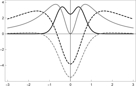
Figure 1: Plots of potential $V_{j}$ (dashed line) and the zero mode associated (solid line). Black line for (64) and gray line for (65).

On the other hand, the behavior of perturbations of the $SO(10)$ self-gravitating domain walls differs from the behavior of the exitations of the $SO(10)$ flat kinks where the $V_{j}$ are Pöschl-Teller potentials Poschl:1933zz ,

$$V_{j_{1}}=2\mu^{2}(3F^{2}-1),\qquad V_{j_{2}}=2\mu^{2}(F^{2}-1).$$ (66)

For each spectrum of scalar states subjected to $V_{j_{1}}$ we find two localized modes

$$m_{0}^{2}=0, \quad\Xi_{0}\sim\cosh^{-2}(ky),$$ (67)

$$m_{1}^{2}=3\mu^{2},\quad \Xi_{1}\sim\cosh^{-2}(ky)\sinh(ky).$$ (68)

While for those ones under $V_{j_{2}}$ only a single state with negative eigenvalue is confined

$$m_{0}^{2}=-\mu^{2},\quad\Xi_{0}\sim\text{sech}(ky).$$ (69)

This reveals the local instability of the symmetric kink when is embedded in a Minkowski spacetime.

When comparing with the $SO(10)$ warped scenario, we noticed that the gravitation repels the tachyonic mode and favors the four-dimensional localization of scalar states $\Xi_{j}(z)$, thus inducing the local stability of the scenario $\mathbf{\Phi_{A}}$.

IV.2 Asymmetric kink

In Section III we showed that on the domain wall $\mathbf{\Phi_{B}}$ the symmetry is broken from $SO(10)$ to the subgroups $SO(6)$, $SU(2)$ and $U(1)$. In particular, along the $SO(6)$ generators we find that the spectrum of scalar perturbations is restricted by $V_{j}$ which depends on (64) or (65). In any case, a tower of states with positive eigenvalues is expected and hence $\mathbf{\Phi_{B}}$ is perturbatively stable in these directions.

On the other hand, for the components of $\Xi_{j}(z)$ along the generators of $SU(2)$ and $U(1)_{\mathbf{P_{B}}}$ we have

$$\frac{\partial^{2}V}{\partial\phi_{j_{3}}^{2}}=4k^{2}\left(1+\frac{4}{9}v^{2}\right);$$ (70)

so, $V_{j_{3}}$ is a positive barrier potential, see Fig.2, which does not support eigenfunctions with $m_{j_{3}}^{2}<0$. Therefore, $\mathbf{\Phi_{B}}$ also is stable along the $SU(2)\otimes U(1)$ generators.

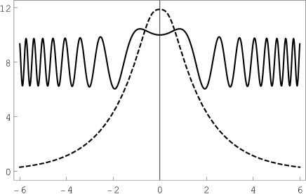
Figure 2: Plots of potential $V_{j_{3}}$ (dashed line) for the scalar perturbations (solid line) of $\mathbf{\Phi_{B}}$ along the $SU(2)\otimes U(1)$ generators.

Now, when the gravity is switched off we find that the scalar perturbation hosted in $SU(2)\otimes U(1)$ are dominated by the potential $V_{j_{3}}=4\mu^{2}>0$ where the eigenvalues are defined for $m^{2}>0$. On the other hand, the wavefunctions associated to $SO(6)$ interact with the potentials (66) and once again within the spectrum of fluctuations there are tachyonic modes (69) induced along the orthogonal subgroup. This puts in evidence the local instability of $\mathbf{\Phi_{B}}$ in five-dimensional Minkowski space.

With regard to the broken generators, for two components of scalar perturbation we find

$$\frac{\partial^{2}V}{\partial\phi_{j_{4}}^{2}}=0$$ (71)

which leads to a symmetric volcano potential for $V_{j_{4}}$ with $m_{j_{4}}\geq 0$ for the eigenfunctions associated. For the others twenty fourth fields we get

$$\frac{\partial^{2}V}{\partial\phi_{j_{\pm}}^{2}}=2k^{2}\left(1+\frac{2}{3}v^{2}(1-\frac{1}{3}F^{2})\right)(F\pm 1)F$$ (72)

and in this case, an asymmetric volcano potentials, $V_{j_{\pm}}$, is obtained. In Fig.3 (top panel) the potential $V_{j_{-}}$ is shown (the profile of the potential $V_{j_{+}}$ is a specular image of the potential $V_{j_{-}}$; thus, both potentials have the same properties). The eigenfunctions are determined by a zero mode localized around the brane and a continuos tower of massive modes propagating freely for the five-dimensional bulk with $m_{-}>0$. Additionally, due to the absence of $Z_{2}$ symmetry in the potential, resonance modes in the spectrum of fluctuations are expected to coexist Gabadadze:2006jm ; Melfo:2010xu ; Araujo:2011fm . Hence, the perturbative stability of AdS₅ vacua along the broken generators is guaranteed and $\mathbf{\Phi_{B}}$ is a stable braneworld.

Let us comment a little further on the symmetry of the potential. For a single scalar field several asymmetric potentials arising from a spacetime without $Z_{2}$ symmetry have been found in Melfo:2002wd ; Guerrero:2005aw . However, in our case the spacetime has $Z_{2}$ symmetry but not $V_{j_{\pm}}$. On the other hand, $\mathbf{\Phi}$ is a $SO(10)$ scalar field self-interacting via $V(\mathbf{\Phi})$, i.e, the components $\phi_{j}$ of the field interact with each other according to the $SO(10)$ symmetry. Therefore, the $SO(10)$ group constrains on the self-interaction of field break the $Z_{2}$ symmetry of the scalar fluctuations along of the broken generators associated to $H_{\mathbf{B}}$.

Figure 3: Plot of the potentials $V_{j_{-}}$ (dashed line) and massive modes (solid line) for scalar perturbations of $\mathbf{\Phi_{B}}$ along the broken generator associated to $H_{\mathbf{B}}$, for the warped geometry (top panel) and flat geometry (bottom panel).

Finally, in the flat scenario, where

$$V_{j_{4}}=0$$ (73)

and

$$V_{j_{\pm}}=2\mu^{2}(F\pm 1)F,$$ (74)

the last one plotted in Fig.3 (botton panel), we notice that the potentials do not support a normalizable zero mode. So, while the gravitation of the scenario delocalized the translation mode, it favours capture of others massless modes, those ones along the broken generatos associated to $\mathbf{H_{B}}$.

IV.3 Superasymmetric kink

The scalar perturbation along $SO(2)$ is the translation mode and, according to what was shown at the beginning of this section, it is not located. In the directions of $SU(4)\otimes U(1)_{\mathbf{P_{C}}}$ we have the quantum mechanics potential (70) for the scalar perturbations. Hence, there are not normalizable massless states along these generators. This also happens in flat case where $V_{j}=4\mu^{2}$ is obtained.

For the broken generators associated to $H_{\mathbf{C}}$, (71) is obtained for twelve scalars and we get (72) for the last sixteen perturbations. Thus, along the broken basis massless bound states are found. Remarkably, in absence of gravity the analogous modes are not normalizable since (73) and (74) are recovered Shin:2003xy .

In any case we do not find modes with $m^{2}<0$ and hence $\mathbf{\Phi_{C}}$ is stable under wall’s perturbations.

V Summary and Conclusions

We have derived three $SO(10)$ self-gravitating kinks interpolating asymptotically between AdS₅ vacuums, such that, whereas the symmetry breaking pattern $SO(10)\rightarrow SU(5)\times Z_{2}$ is induced at the edges of the scenarios, in the core of each wall, a different unbroken symmetry is obtained: $SO(10)$, $SO(6)\otimes SU(2)\otimes U(1)/Z_{2}$ and $SU(4)\otimes SO(2)\otimes U(1)/Z_{4}$ respectively for the symmetric, asymmetric and superasymmetric kink.

These solutions are the gravitational analogue of the $SO(10)$ walls in Minkowskian bulk found in Shin:2003xy . The perturbative stability of scenarios were studied and as a result we find that gravitation favors the stability of the $SO(10)$ walls and its absence, on the contrary, weakens the integrity of the scenarios. In flat case, in addition to four-dimensional translation mode, massive states and tachyonic Pöschl-Teller states along $SO(10)$ and $SO(6)$ for the symmetric and asymmetric kink respectively are obtained in the spectrum of the scalar fluctuations. Fortunately, when gravity is included, the unstable tachyonic excitations are not already present and the scalar perturbation spectrum is defined only for $m^{2}\geq 0$.

The scalar fluctuations of the non-abelian warped scenarios satisfy the following general characteristics: free massive modes ($m^{2}>0$), non-normalizable translation mode and localized massless states along broken generators associated to $\mathbf{H_{0}}$ (Nambu-Goldstone bosons). These gravitational effects on the scalar fluctuations are fulfilled by the superasymmetric kink.

Now, for the symmetric and asymmetric kink, in addition to Nambu-Goldstone bosons, massless scalar excitations along the orthogonal subgroup are confined. The results are summered as follow: For the symmetric scenario, we find $SO(10)$ scalar zero modes trapped by the wall. This effect also is shared by the asymmetric scenario where scalar massless fluctuations along the generators of $SO(6)$ are localized. In both cases tachyonic modes are not found. Hence, the unstable modes along the orthogonal groups found in flat case are shifted for bounded zero modes when gravity is included.

Finally, we observe that the interactions conditioned by the orthogonal symmetry, unlike those ones defined by unitary group, could be favoring the confinement of spinless bosons along the unbroken generators of $\mathbf{H_{0}}$. This issue is beyond the scope of this paper and will be treated in a next work.

VI Acknowledgements

We wish to thank Rafael Torrealba and Oscar Castillo-Felisola for discussions. This work was supported by CDCHT-UCLA under projects 007-RCT-2014 and 03-CT-2015.

VII Appendix

In $N$ dimensions one can define $N(N-1)/2$ linearly independent and antisymmetric matrices $\mathbf{L}$ to form a basis such that any real antisymmetric $N\times N$ matrix can be expanded in terms of this basis. The Lie algebra for the basis $\mathbf{L}$ is given through

$$[\mathbf{L}_{j_{1}j_{2}},\mathbf{L}_{j_{3}j_{4}}]= \delta_{j_{1}j_{4}}\mathbf{L}_{j_{2}j_{3}}-\delta_{j_{1}j_{3}}\mathbf{L}_{j_{2}j_{4}}$$ (75)

$$+\delta_{j_{2}j_{3}}\mathbf{L}_{j_{1}j_{4}}-\delta_{j_{2}j_{4}}\mathbf{L}_{j_{1}j_{3}},$$

where $j=1,\dots,N$. The mutually commuting generators can be found and they are $\mathbf{L}_{12}$, $\mathbf{L}_{34},\dots,\mathbf{L}_{N-1,N}$. These generators form an abelian subgroup i.e., the Cartan subalgebra of $SO(N)$. The rank of the algebra is equal to the number of mutually commuting generators.

A suitable generating expression for the basis $\mathbf{L}$ can be stated as

$$\left(\mathbf{L}_{j_{1}j_{2}}\right)_{j_{3}j_{4}}=\delta_{j_{1}j_{4}}\delta_{j_{2}j_{3}}-\delta_{j_{1}j_{3}}\delta_{j_{2}j_{4}}.$$ (76)

In particular, for $N=10$ we deal with three kink solutions for the scalars field $\mathbf{\Phi}$ and to find explicitly the remain symmetry in the core of each kink we introduce three differently basis, A,B,C, obtained from a certain combination of ${\mathbf{L}}$’s.

Basis A: for the symmetric scenario

$$\mathbf{T_{A}}^{1} = \mathbf{M_{A}},$$ (77)

$$\mathbf{T_{A}}^{2}=\frac{1}{\sqrt{20}}(\mathbf{L}_{34}+\mathbf{L}_{56} + \mathbf{L}_{78}+\mathbf{L}_{90}-4\mathbf{L}_{12}),$$ (78)

$$\mathbf{T_{A}}^{3}={\frac{1}{\sqrt{12}}}(\mathbf{L}_{56}+ \mathbf{L}_{78} +\mathbf{L}_{90}-3\mathbf{L}_{34}),$$ (79)

$$\mathbf{T_{A}}^{4}=\frac{1}{\sqrt{6}}(\mathbf{L}_{78} + \mathbf{L}_{90}-2\mathbf{L}_{56}),$$ (80)

$$\mathbf{T_{A}}^{5}=\frac{1}{\sqrt{2}}( \mathbf{L}_{90} -2\mathbf{L}_{78}).$$ (81)

Basis B: for the asymmetric kink

$$\mathbf{T_{B}}^{1}=\mathbf{M_{B}},\quad\mathbf{T_{B}}^{2} = \frac{1}{\sqrt{6}}(-2\mathbf{L}_{12}+\mathbf{L}_{34}+\mathbf{L}_{56}),$$ (82)

$$\mathbf{T_{B}}^{3}=\frac{1}{\sqrt{2}}( \mathbf{L}_{34} -\mathbf{L}_{56}),\quad\mathbf{T_{B}}^{4}=\mathbf{P_{B}}$$ (83)

$$\mathbf{T_{B}}^{5} = \frac{1}{\sqrt{2}}(\mathbf{L}_{78}-\mathbf{L}_{90}).$$ (84)

Basis C: for superasymmetric case

$$\mathbf{T_{C}}^{1}=\mathbf{M_{C}} \mathbf{T_{C}}^{2}=\mathbf{P_{C}},$$ , (85)

$$\mathbf{T_{C}}^{3}=\frac{1}{\sqrt{12}}(-3\mathbf{L}_{34} + \mathbf{L}_{56}+\mathbf{L}_{78}+\mathbf{L}_{90}),$$ (86)

$$\mathbf{T_{C}}^{4}=\frac{1}{\sqrt{6}}(\mathbf{L}_{78} + \mathbf{L}_{90}-2\mathbf{L}_{56}),$$ (87)

$$\mathbf{T_{C}}^{5}=\frac{1}{\sqrt{2}}( \mathbf{L}_{78} -\mathbf{L}_{90}).$$ (88)

These basis share forty generators which are determined by

$$\mathbf{T}^{j^{\prime}}=\frac{1}{\sqrt{2}}C^{j^{\prime}}_{ij}\mathbf{L}_{ij},\quad{j^{\prime}}=6,\dots,45,$$ (89)

where $1/\sqrt{2}$ is a normalization factor and $C^{j^{\prime}}_{ij}$ a linear combination coefficient which is selected according to

$$\begin{array}[]{c l l}&{j^{\prime}}=10+j,&j\;\text{even}\\ C^{j^{\prime}}_{1j}=1,&{j^{\prime}}=12+j,&j\;\text{odd}\\ &{j^{\prime}}=3+j,&\text{for all}\;j;\end{array}$$

$$\begin{array}[]{c l l}&{j^{\prime}}=22+j,&j\;\text{even}\\ C^{j^{\prime}}_{3j}=1,&{j^{\prime}}=24+j,&j\;\text{odd}\\ &{j^{\prime}}=17+j,&\text{for all}\;j;\end{array}$$

$$\begin{array}[]{c l l}&{j^{\prime}}=30+j,&j\;\text{even}\\ C^{j^{\prime}}_{5j}=1,&{j^{\prime}}=32+j,&j\;\text{odd}\\ &{j^{\prime}}=27+j,&\text{for all}\;j,\end{array}$$

for $10\geq j>i+1$;

$$\begin{array}[]{c}C^{j^{\prime}}_{2j}=\left\{\begin{array}[]{lll}1,&{j^{\prime}}=2+j,&j\;\text{even}\\ &{j^{\prime}}=4+j,&j\;\text{odd}\\ -1,&{j^{\prime}}=11+j,&\text{for all}\;j;\end{array}\right.\end{array}$$

$$\begin{array}[]{c}C^{j^{\prime}}_{4j}=\left\{\begin{array}[]{lll}1,&{j^{\prime}}=16+j,&j\;\text{even}\\ &{j^{\prime}}=18+j,&j\;\text{odd}\\ -1,&{j^{\prime}}=23+j,&\text{for all}\;j;\end{array}\right.\end{array}$$

$$\begin{array}[]{c}C^{j^{\prime}}_{6j}=\left\{\begin{array}[]{lll}1,&{j^{\prime}}=26+j,&j\;\text{even}\\ &{j^{\prime}}=28+j,&j\;\text{odd}\\ -1,&{j^{\prime}}=31+j,&\text{for all}\;j\end{array}\right.\end{array}$$

for $10\geq j>i$ and

$$C^{42}_{70}=C^{45}_{79}=-1$$

$$C^{43}_{74}=C^{44}_{70}=C^{42}_{89}=C^{43}_{80}=C^{44}_{89}=C^{45}_{80}=1.$$

To indicate the unbroken symmetry group on the wall, we will focus on getting the basis that annihilate the field in the core, $[{\mathbf{T}},{\mathbf{\Phi}}(y=0)]=0$. For $\mathbf{\Phi_{A}}$ the result is straightforward because all generators annihilate to $\mathbf{\Phi_{A}}(y=0)$ and, therefore, the $SO(10)$ symmetry is restored on the kink.

For the asymmetric scenario $\mathbf{\Phi_{B}}$, there are nineteen generators annihilating the field in the origin of which fifteen of them form a basis for $SO(6)$ ($j=1$, 2, 3, 6, 7, 8, 9, 14, 15, 16, 17, 22, 23, 28, 29), three of them ($j=5$, 42, 43) are generators of $SO(3)\sim SU(2)$ and the last one, $j=4$, in correspondence with $SO(2)\sim U(1)$. Hence, on the asymmetric kink $SO(10)\rightarrow SO(6)\otimes SU(2)\otimes U(1)/Z_{2}$ is obtained.

Finally, with respect to the superasymmetric kink $\mathbf{\Phi_{C}}$ we have seventeen generators annihilating the field in $y=0$. In this case, fifteen of them ($j=3$, 4, 5, 22, 24, 26, 28, 30, 32, 34, 36, 38, 40, 42, 43) are associated to $SO(6)\sim SU(4)$ and the two remaining ones ($j=1,2$) are in correspondence with $SO(2)$ and with $SO(2)\sim U(1)$. Therefore, $SO(10)\rightarrow SU(4)\otimes SO(2)\otimes U(1)/Z_{4}$ is recovered in the core of the scenario.

Notice that, the unbroken symmetries $SO(6)\otimes SU(2)\otimes U(1)$ and $SU(4)\otimes SO(2)\otimes U(1)$ are closely related with the Pati-Salam like group, $SU(4)\otimes SU(2)\otimes U(1)$, and the chiral bilepton gauge model, $SU(4)\otimes U(1)\otimes U(1)$, respectively.

References

• (1) L. Randall and R. Sundrum, Phys. Rev. Lett.  83, 4690 (1999)
• (2) B. Bajc and G. Gabadadze, Phys. Lett. B 474, 282 (2000)
• (3) G. R. Dvali, G. Gabadadze and M. A. Shifman, Phys. Lett. B 497, 271 (2001)
• (4) O. DeWolfe, D. Z. Freedman, S. S. Gubser and A. Karch, Phys. Rev. D 62, 046008 (2000)
• (5) M. Gremm, Phys. Lett. B 478, 434 (2000)
• (6) A. Wang, Phys. Rev. D 66, 024024 (2002)
• (7) D. Bazeia, C. Furtado and A. R. Gomes, JCAP 0402, 002 (2004)
• (8) A. Melfo, N. Pantoja and A. Skirzewski, Phys. Rev. D 67, 105003 (2003)
• (9) O. Castillo-Felisola, A. Melfo, N. Pantoja and A. Ramirez, Phys. Rev. D 70, 104029 (2004)
• (10) A. Melfo, N. Pantoja and J. D. Tempo, Phys. Rev. D 73, 044033 (2006)
• (11) R. Guerrero, A. Melfo, N. Pantoja and R. O. Rodriguez, Phys. Rev. D 74, 084025 (2006)
• (12) R. Guerrero, A. Melfo, N. Pantoja and R. O. Rodriguez, Phys. Rev. D 81, 086004 (2010)
• (13) M. Giovannini, Phys. Rev. D 64 (2001) 064023
• (14) D. P. George, Phys. Rev. D 83, 104025 (2011)
• (15) A. Melfo, R. Naranjo, N. Pantoja, A. Skirzewski and J. C. Vasquez, Phys. Rev. D 84, 025015 (2011)
• (16) L. Pogosian and T. Vachaspati, Phys. Rev. D 62, 123506 (2000)
• (17) T. Vachaspati, Phys. Rev. D 63, 105010 (2001)
• (18) L. Pogosian, Phys. Rev. D 65, 065023 (2002)
• (19) T. Vachaspati, Phys. Rev. D 67, 125002 (2003)
• (20) A. Davidson, D. P. George, A. Kobakhidze, R. R. Volkas and K. C. Wali, Phys. Rev. D 77, 085031 (2008)
• (21) N. Pantoja and R. Rojas, arXiv:1511.08089 [hep-th].
• (22) E. M. Shin and R. R. Volkas, Phys. Rev. D 69, 045010 (2004)
• (23) L. F. Li, Phys. Rev. D 9, 1723 (1974).
• (24) J. M. Bardeen, Phys. Rev. D 22, 1882 (1980). doi:10.1103/PhysRevD.22.1882
• (25) N. Arkani-Hamed and M. Schmaltz, Phys. Rev. D 61, 033005 (2000) doi:10.1103/PhysRevD.61.033005 [hep-ph/9903417].
• (26) M. Shaposhnikov, P. Tinyakov and K. Zuleta, JHEP 0509, 062 (2005)
• (27) G. Poschl and E. Teller, Z. Phys.  83, 143 (1933).
• (28) G. Gabadadze, L. Grisa and Y. Shang, JHEP 0608, 033 (2006) doi:10.1088/1126-6708/2006/08/033 [hep-th/0604218].
• (29) A. Melfo, N. Pantoja and F. Ramirez, arXiv:1011.2524 [hep-th].
• (30) A. Araujo, R. Guerrero and R. O. Rodriguez, Phys. Rev. D 83, 124049 (2011) doi:10.1103/PhysRevD.83.124049 [arXiv:1104.3627 [hep-th]].
• (31) R. Guerrero, R. O. Rodriguez and R. S. Torrealba, Phys. Rev. D 72, 124012 (2005)