Towards Self-Calibrating Inertial Body Motion Capture

Abstract

This paper presents a novel online capable method for simultaneous estimation of human motion in terms of segment orientations and positions along with sensor-to-segment calibration parameters from inertial sensors attached to the body. In order to solve this ill-posed estimation problem, state-of-the-art motion, measurement and biomechanical models are combined with new stochastic equations and priors. These are based on the kinematics of multi-body systems, anatomical and body shape information, as well as, parameter properties for regularisation. This leads to a constrained weighted least squares problem that is solved in a sliding window fashion. Magnetometer information is currently only used for initialisation, while the estimation itself works without magnetometers. The method was tested on simulated, as well as, on real data, captured from a lower body configuration.

I INTRODUCTION

Inertial body motion capture (mocap) has found widespread use in various applications ranging from robotics [1] over sports [2] and health [3, 4] to human-machine-interaction [5]. In particular if in-field assessment of human motion is required, body-worn inertial measurement units (IMUs), including 3D accelerometers, gyroscopes and often magnetometers, offer key advantages over marker-based optical systems [6], by not depending on the line of sight or being restricted to laboratory conditions. Though mature systems are already available on the market [7], inertial mocap is still subject of research aiming at both increasing the accuracy, robustness, as well as, the practicality of such systems. One challenge that arises for magnetometer dependent systems is the fact that man made environments do often not provide a static magnetic field, thus reduced dependence on magnetometer usage represents an important aspect of robustness [8]. Moreover, in order to deduce the positions and orientations of the body segments comprising the biomechanical model via body-worn IMUs, it is crucial to know the relative position and orientation of each IMU with respect to (w.r.t.) the segment it is attached to (cf. Fig. 1). In a kinematic model with rigid segments and joints, the IMU-to-segment relation (I2S calibration) is typically modelled as a rigid transformation with six degrees of freedom (DoF) [7, 9, 10, 11, 12]. Providing accurate and easy-to-use calibration mechanisms is therefore an important aspect of practicality.

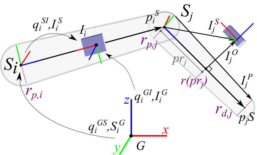
Figure 1: Biomechanical model with two segments.

Though I2S calibration errors, in particular w.r.t. the orientations, immediately lead to errors within the estimated segment poses [13, 14], calibration issues have not been intensively addressed in the mocap literature, i.e. calibration is often assumed to be given, e.g. [12, 10]. Functional calibration requires the user to precisely perform predefined static poses or movements. The most simple but also widespread procedures involve only one static pose, e.g. the so-called N-pose (all segments aligned with the vertical) or T-pose (arm segments horizontal), from which all I2S orientations can be determined based on measured accelerations and magnetic fields [7].

Note that human anatomy does not allow to precisely perform the N-pose, for instance, due to the individual’s carrying angle, chest and upper arm circumferences, which all influence the calibration result [15]. Calibration procedures based on measuring angular velocities during rotations around predefined anatomical axes result in better consistency with anatomical joint coordinate systems [13]. However, they usually involve more steps and are less easy to perform by a subject autonomously [16], [13]. In [17], different manual alignment and functional calibration methods, including the above mentioned ones, are validated against an optoelectronic reference system based on ten healthy subjects instructed by three operators. The study reports precision in the range $[6,26]^{\circ}$ and reproducibility in the range $[5,10]^{\circ}$ root mean squared error (RMSE). It is pointed out that calibration accuracy is more dependent on the level of rigor of the experimental procedure (e.g. the operator training) than on the choice of calibration itself. This underlines the limitation of these methods to require a trained and compliant user, who, in addition, has the physical and cognitive capabilities to precisely perform the required protocol.

Self-calibration methods determine calibration parameters from sensor measurements without prior knowledge or assumptions about the performed movements and are therefore particularly interesting when targeting a practical system. Up to now, such methods appear to be mainly used for calibrating single sensor units or packages, in particular when estimating calibration parameters simultaneously with motion; e.g. [18] proposes an offline maximum likelihood estimator for simultaneous IMU calibration and orientation estimation during arbitrary motion, while [19] proposes an extended Kalman filter based method for simultaneous vehicle navigation and smartphone-to-vehicle alignment. In the recent robotics literature, several examples of online [20] and offline [21, 22] estimation of calibration parameters simultaneously with motion can be found. However, self-calibration methods for human motion tracking appear to be rare. In [23], offline least squares estimators are proposed for estimating calibration parameters of two linked segments with attached IMUs from their measured angular velocities and accelerations. Parameters include the rotation axis of a revolute joint (e.g. the knee) and the position of a ball-and-socket joint, given in the reference frames of the two IMUs. In [24] the IMU position calibration method of [23] is initially analyzed w.r.t. observability and additional constraints from a three-link-segment are introduced in order to better constrain the optimisation problem.

Removing the need for precisely executing predefined calibration poses or movements, in particular when IMUs have slipped unintentionally during recording, is a key requirement for obtaining a truly practical system, which can be operated by a wide range of non-expert users. The present work makes a first step into this direction by showing results from a novel online-capable, self-calibrating inertial body mocap system. The approach is inspired by the offline inertial mocap method of [12] that obtains a constrained weighted least squares (WLS) estimate for a complete movement from a batch of inertial measurements. In this paper, a sliding window based constrained WLS method is proposed for simultaneously estimating the body motion along with the I2S calibration parameters. The approach can also be used as a moving horizon approach, thus avoiding a delay in processing streamed data [25]. In order to achieve convergence from a wide range of initialisations, new stochastic equations and priors are introduced into the objective function. These are based on multi-body kinematic equations [11], anatomical information (restricted joints and range of motion), similar to [10], and novel inclusion of body shape information as well as regularisation. The convergence behaviour, precision and repeatability of the proposed method were initially tested within both, a simulation study and a real data case study, where a subject performed squat exercises. On simulated data from a two segment model, reliable convergence with sub-degree precision was observed when initialising the I2S orientations with angular offsets up to $95^{\circ}$. On real data captured from a lower body with four segments, repeatable results (below $2^{\circ}$ difference) were obtained from three different initialisations of the sensor-to-segment calibrations including a maximum initial angular difference of $113^{\circ}$. In the following, Section II introduces the notation, while Sections III through V explain the proposed method, which is then evaluated in Sections VI and VII. Finally, Section VIII draws conclusions.

II Notation and Biomechanical Model

As illustrated in Fig. 1, the human body is represented as a set of rigid segments $\mathbb{S}$ that are connected through joints, $\mathbb{J}$. For each joint, $J_{k}\in\mathbb{J}$, the connecting segments are collected in $\mathbb{S}_{J_{k}}$. A subset $\mathbb{H}\subset\mathbb{J}$ is assumed to be hinge joints (e.g. the knee has one major rotation axis, which is in general not aligned with any of the local segment frame axes [23]) with limited range of motion (RoM), while the other joints are modelled as ball-and-socket joints. Inspired by the Hanavan model [26], each segment $S_{i}\in\mathbb{S}$ is surrounded by a capsule $C_{i}\in\mathbb{C}$, which represents the soft tissue.

A set of IMUs $\mathbb{I}$ is attached to the body, where $I_{i}\in\mathbb{I}$ is assumed to be on segment $S_{i}$, sitting on the surface of $C_{i}$. Each segment $S_{i}\in\mathbb{S}$ has a local frame attached to it, with the origin in the centre of rotation of the proximal joint and the $z$-axis pointing along the segment. The segment pose w.r.t. the global frame $G$ is parametrized through an orientation quaternion $q^{GS}_{i}$ and a position $S_{i}^{G}$. The segment vector, $p^{S}_{i}$, points along the segment from the proximal to the distal joint or endpoint, where $\|p^{S}_{i}\|$ corresponds to the segment length. The surrounding capsule $C_{i}$ has radii $r_{p,i}$ and $r_{d,i}$ at the proximal and distal joint, respectively. Note that $r_{d,i}$ is equivalent with $r_{p,i}$ of the subsequent segment in distal direction. Each IMU $I_{i}$ has a local frame attached to it, with origin in the centre of the accelerometer triad, coordinate axes aligned to the casing and local $z$-axis pointing orthogonally away from the bottom plate. The IMU’s orientation and position w.r.t. to $G$ are denoted $q^{GI}_{i}$ and $I_{i}^{G}$, respectively. The I2S calibrations are defined as the relative orientations $q^{SI}_{i}$ and positions $I_{i}^{S}$, $\forall I_{i}\in\mathbb{I}$.

The knowledge required by the proposed method comprises segment lengths, capsule radii, hinge rotation axes and ranges of motion. These can be obtained based on measurements in combination with anthropometric databases [27, 26], body scanning technologies [28, 29] or calibration [23] and have to be determined once per person.

In the following, unit quaternion $q$ and respective rotation matrix $R$ are used interchangeably.

III Variables, motion and measurement models

The variables to be estimated include:

• IMU poses and velocities for each time step $t$: $I^{G}_{i,t},\dot{I}^{G}_{i,t}q^{GI}_{i,t},\omega^{GI}_{I,i,t},\forall I_{i}\in\mathbb{I}$

• Segment poses for each time step $t$: $S^{G}_{i,t},q^{GS}_{i,t},\forall S_{i}\in\mathbb{S}$

• I2S calibrations: $I_{i}^{S},q^{SI}_{i},\forall I_{i}\in\mathbb{I}$.

Note, the general approach of defining a redundant variable set in combination with constraints, rather than relying on a minimal parametrisation (e.g. [9], [30]) is adopted from [12], arguing that this better accounts for model violations typically appearing in human motion tracking, (e.g. due to soft tissue artefacts and anatomical variability).

Note, gyroscope and accelerometer bias models are not in the focus of this paper, but can be easily added, see e.g. [12, 31].

The motion of each IMU $I_{i}\in\mathbb{I}$ from time step $t$ to $t+1$, with sampling time $T$, is modelled by taking the measured acceleration, $y^{a}_{i,t}$, as input [31], yielding $\forall I_{i}\in\mathbb{I}$:

$$I^{G}_{i,t+1} =I^{G}_{i,t}+T\dot{I}^{G}_{i,t}+\frac{T^{2}}{2}R^{GI}_{i,t}(y^{a}_{i,t}-v^{I^{G}}_{i,t})+\frac{T^{2}}{2}g^{G},$$ (1a)

$$\dot{I}^{G}_{i,t+1} =\dot{I}^{G}_{i,t}+TR^{GI}_{i,t}\left(y^{a}_{i,t}-v^{\dot{I}^{G}}_{i,t}\right)+Tg^{G},$$ (1b)

$$q^{GI}_{i,t+1} =q^{GI}_{i,t}\odot\exp\left(\frac{T}{2}\omega^{GI}_{I,i,t}+v^{q^{GI}}_{i,t}\right),$$ (1c)

with process noises $v^{X}_{i,t}\sim\mathcal{N}(0,\Sigma^{X}),\,X\in\{I^{G},\dot{I}^{G},q^{GI}\}$. Here, $g^{G}$ denotes the global gravity vector, $\odot$ and $\exp$ are the quaternion product and exponential, respectively.

For all $I_{i}\in\mathbb{I}$ the measured angular velocity, $y^{\omega}_{i,t}$, is related to the estimated angular velocity via [31]:

$$y^{\omega}_{i,t}=\omega^{GI}_{I,i,t}+e^{y^{\omega}}_{i,t},\quad e^{y^{\omega}}_{i,t}\sim\mathcal{N}(0,\Sigma^{y^{\omega}}).$$ (2)

The reason for modelling the measured accelerations as inputs and the angular velocities as measurements is that both angular and linear velocities are required as estimation variables (cf. Section IV-B).

IV Biomechanical model and priors

In the following, the biomechanical model is formulated as constraints, stochastic equations and priors for the final WLS minimisation. Here, priors correspond to equations that include the I2S calibration parameters only.

IV-A Connected segments constraint and I2S calibration

These relations are adapted from [12] and are included as follows. $\forall J_{k}\in\mathbb{J}$ with $S_{i},S_{j}\in\mathbb{S}_{J_{k}}$:

$$c(S_{j,t}^{G},S_{i,t}^{G},q^{GS}_{i,t})=S_{j,t}^{G}-\left(S_{i,t}^{G}+R^{GS}_{i,t}(p^{S}_{i})\right).$$ (3)

This constrains the body segments to be attached at the joints. Moreover, $\forall I_{i}\in\mathbb{I}$:

$$q^{GI}_{i,t} =q^{GS}_{i,t}\odot q^{SI}_{i,t}\odot\exp\left(\frac{1}{2}e^{q^{SI}}_{i,t}\right),e^{q^{SI}}_{i,t}\sim\mathcal{N}(0,\Sigma^{q^{SI}}),$$ (4a)

$$I_{i,t}^{G} =S_{i,t}^{G}+R^{GS}_{i,t}\left(I^{S}_{i,t}+e^{I^{S}}_{i,t}\right),e^{I^{S}}_{i,t}\sim\mathcal{N}(0,\Sigma^{I^{S}}),$$ (4b)

models the fact that IMU and segment poses are coupled through the I2S calibrations, up to some uncertainty that might compensate for soft-tissue artefacts [12].

IV-B Velocity at joints

In [11], a measurement model for minimising the linear velocity difference at a joint was proposed in a filter framework. The goal was to reduce the dependence on magnetometer usage for heading drift correction. In this work we found that this minimisation aids the calibration estimation (cf. Fig. 4). The equation can be adapted as follows. $\forall J_{k}\in\mathbb{J}$ with $S_{i},S_{j}\in\mathbb{S}_{J_{k}}$, $I_{i},I_{j}\in\mathbb{I}$:

$$e^{J_{v}}_{k,t}=\dot{I}_{i,t}^{I}+\omega_{I,i}^{GI}\times\left(R^{IS}_{i}(p_{i}^{S_{i}}-I_{i}^{S_{i}})\right)\\ -R^{IG}_{i}R^{GI}_{j}\left(\dot{I}_{j,t}^{I}+(R^{IS}_{j}I_{j}^{S})\times\omega_{I,j}^{GI}\right),\quad e^{J_{v}}_{k,t}\sim\mathcal{N}(0,\Sigma^{J_{v}}).$$ (5)

IV-C Hinge joint and RoM limit

Minimising $\forall J_{k}\in\mathbb{H}$ with $S_{i},S_{j}\in\mathbb{S}_{J_{k}}$:

$$e^{H}_{k,t}=h^{S}_{i}-R^{SG}_{j,t}R^{GS}_{i,t}h^{S}_{i},\quad e^{H}_{k,t}\sim\mathcal{N}(0,\Sigma^{H}),$$ (6a)

constrains the rotation of joint $$J_{k} h^{S}_{i} e^{H}_{k,t} \text{{RoM}\@}\in[\theta_{min,k},\theta_{max,k}]$$ to mainly appear around axis , which is assumed known (cf. Section II). Here, the additive noise term accounts for both, an error in the rotation axis and small rotations around other axes. Moreover, rotation angles around this axis outside a predefined range, , are penalised by minimising:

$$e^{RoM}_{k,t}=\begin{cases}\theta_{min,k}-\theta_{k,t}&\text{for }\theta_{k,t}<\theta_{min,k}\\ \theta_{k,t}-\theta_{max,k}&\text{for }\theta_{k,t}>\theta_{max,k}\\ 0&\text{otherwise },\end{cases}$$ (6b)

with $\theta_{k,t}=2\arccos([q^{SG}_{j,t}\odot q^{GS}_{i,t}]_{w})$ and $e^{RoM}_{k,t}\sim\mathcal{N}(0,\Sigma^{RoM})$.

IV-D Body shape prior

Assuming each IMU to be mounted approximately on the surface of the respective body segment, approximated via a capsule (cf. Fig. 1), is a reasonable assumption that can be used to guide both the I2S orientation and position estimation. As illustrated in Fig. 1, let $pr_{i,t}$ be the length of the orthogonal projection of IMU position $I^{S}_{i}$ onto the segment $p^{S}_{i}$, and let $I^{O}_{i}$ be the vector part of $I^{S}_{i}$ which is orthogonal to the segment. Minimising, $\forall I_{i}\in\mathbb{I}$:

$$e^{I^{S}_{shape}}_{i}=\begin{cases}I^{S}_{i}-r_{p,i}\overline{I^{S}_{i}}&\text{for }pr_{i}<0\\ I^{O}_{i}-r(pr_{i})\overline{I^{O}_{i}}&\text{for }0\leq pr_{i}\leq\|p^{S_{i}}\|\\ (I^{S}_{i}-p^{S}_{i})-r_{d,i}\overline{I^{S}_{i}-p^{S}_{i}}&\text{for }pr_{i}>\|p^{S}_{i}\|,\end{cases}$$ (7a)

with $$\overline{v}\coloneqq\frac{v}{\|v\|} r(pr_{i})\coloneqq r_{p,i}+\frac{pr_{i}}{\|p^{S}_{i}\|}(r_{d,i}-r_{p,i}) e^{I^{S}_{shape}}_{i}\sim\mathcal{N}(0,\Sigma^{I^{S}_{shape}}) I^{S}_{i,t} r(pr_{i}) I^{P}_{i}$$, and allows to move on the surface of the capsule while penalising orthogonal displacements. The above model can be extended to other shapes by modifying the computation of the radius . Even more complex shapes (e.g. from a body scanner) could be included, given that the complete surface and outer normals of the shape are known. Moreover, as illustrated in Fig. 1, let be a vector parallel to the capsule surface. Minimising:

$$e^{q^{SI}_{shape}}_{i}=[R^{SI}_{i}]_{3,1:3}\overline{I_{i}^{P}},\quad e^{q^{SI}_{shape}}_{i}\sim\mathcal{N}(0,\Sigma^{q^{SI}_{shape}}),$$ (7b)

constrains the IMU’s $z$-axis to point orthogonally to the capsule surface. Here, $R_{3,1:3}$ picks the third row of the rotation matrix $R$. Without loss of generality, we assume here that the $z$-axis of the IMU points away from the surface it is mounted on. The positive effect of this prior can be observed in Fig. 4. Note, this prior only depends on the calibration parameters and is therefore not time dependent.

IV-E Fixed segment position

In some movement scenarios, it is known that some segments are stationary at specific points, e.g. that the soles of the feet stay on the ground. Let $\mathbb{F}\subset\mathbb{S}$ define a subset of segments with fixed position. Minimising, $\forall S_{i}\in\mathbb{F}$:

$$e^{S^{G}_{fix}}_{i,t}=p^{G}_{i,fix}-\left(S^{G}_{i,t}+R^{GS}_{i,t}p^{S}_{i,fix}\right),e^{S^{G}_{fix}}_{i,t}\sim\mathcal{N}(0,\Sigma^{S^{G}_{fix}})$$ (8)

constrains the fixed position $p^{S}_{i,fix}$ to coincide with the known global position $p^{G}_{i,fix}$ at each time step $t$. Alternative methods to reduce drift are, for instance, to enforce zero velocity based on detections [32] or to enforce a known mean acceleration [12].

V Sliding window based optimisation

In [12] it is suggested to calculate an offline maximum a posteriori (MAP) estimate of the IMU and segment poses of all time steps, by solving a global constrained WLS problem, where (3) enters as hard equality constraints. In order to reduce the computation time, the optimisation works on accumulated measurement data. Moreover, the I2S calibrations are assumed known. In order to obtain an online-capable approach a sliding window based WLS estimate is proposed in this work. It sequentially processes overlapping batches of few IMU data as they are captured, in order to estimate both kinematics and I2S calibrations. Let $\{y^{a},y^{\omega}\}_{t=0:w-1}^{b},w\geq 2$ be the sequence of IMU data available in batch $b\geq 0$, with $y_{t}\coloneqq[y^{a},y^{\omega}]_{t}^{T}$. Moreover, for $b>0$, let $\{y^{a},y^{\omega}\}_{w-1}^{b-1}=\{y^{a},y^{\omega}\}^{b}_{0}$, i.e. let the last time step of batch $b-1$ correspond to the first time step in batch $b$, so that each new batch contains $w-1$ new time steps and the size of each batch is $w$. Then, the variables to be estimated for batch $b$ comprise (cf. Section III): time-varying IMU kinematics and segment poses:

$$x^{b} =\left\{\left\{I^{G}_{i,t},\dot{I}^{G}_{i,t}q^{GI}_{i,t},\omega^{GI}_{I,i,t}\right\}_{I_{i}\in\mathbb{I}},\left\{S^{G}_{i,t},q^{GS}_{i,t}\right\}_{S_{i}\in\mathbb{S}}\right\}_{t=0:w-1}^{b}$$ (9a)

and static I2S calibrations

$$z^{b} =\left\{I_{i}^{S},q^{SI}_{i}\right\}_{I_{i}\in\mathbb{I}}^{b}.$$ (9b)

Overall this gives the following dimensionality for the state per batch $[x^{b},z^{b}]^{T}\in\mathbb{R}^{w(13|\mathbb{I}|+7|\mathbb{S}|)+7|\mathbb{I}|}$.

V-A Batch initialisation and regularisation

Measurement noise, model errors and motion that is available in the small batches can significantly influence the estimation result and cause instant changes in both the estimates of the time-varying variables at the batch overlap and the estimated I2S calibrations. These are $x_{w-1}^{b-1}$, $x_{0}^{b}$ and $z^{b-1}$, $z^{b}$, respectively. To reduce this effect, different regularisation priors are introduced. Minimising $\forall I_{i}\in\mathbb{I}$

$$e^{q^{GI}_{0}}_{i,t}=\begin{cases}2\log\left(q^{IG,b-1}_{i,w-1}\odot q^{GI,b}_{i,0}\right)&\text{for }b>0\\ 2\log\left(q^{IG}_{i,init}\odot q^{GI,b}_{i,0}\right)&\text{else }\end{cases},$$ (10)

with $e^{q^{GI}_{0}}_{i,t}\sim\mathcal{N}(0,\Sigma^{q^{GI}_{0}})$ penalises sudden changes of the estimated IMU orientations for the overlap of $b-1$ and $b$. Note, in a moving horizon context this term corresponds to the arrival cost for the variables. Here, $\log$ denotes the quaternion logarithm. Note, for $b=0$ the initial quaternions $q^{GI}_{i,init}$ are obtained using the TRIAD algorithm [33]. This is currently the only point, where magnetometer data is used in the proposed method. Regularising only the initial IMU orientations in each batch turned out to be sufficient to produce a smooth trajectory.

Moreover, for $b>0$ and $\forall I_{i}\in\mathbb{I}$, minimising

$$e^{q^{SI}_{const}}_{i} =\log\left(q^{IS}_{i,b-1}\odot q^{SI}_{i,b}\right),\quad e^{q^{SI}_{const}}_{i}\sim\mathcal{N}(0,\Sigma^{q^{SI}_{const}})$$ (11a)

$$e^{I^{S}_{const}}_{i} =I^{S}_{i,b}-I^{S}_{i,b-1},\quad e^{I^{S}_{const}}_{i}\sim\mathcal{N}(0,\Sigma^{I^{S}_{const}})$$ (11b)

penalises sudden changes in the I2S calibrations between batch $b-1$ and $b$. Obviously, the amount of change depends on the noise covariances, which have to be adapted appropriately in order to enable convergence to a stationary or only slightly varying calibration, i.e. the correct one.

For this, a convergence indicator has been defined based on the following observations: First, in the presence of motion, the residuals of the velocity constraint are biased, if one or both of the respective I2S calibrations are incorrect. Second, if an I2S calibration stays rather constant over a history of $h$ batches, despite motion and high covariances in (11), a feasible calibration is indicated. Hence, if:

$$\frac{1}{w}\frac{1}{|\mathbb{J}|}\left\|\sum_{t=0}^{w-1}\sum_{k\in\mathbb{J}}\left(e^{J_{v}}_{k,t}\right)^{b}\right\|_{2}<th^{J_{v}}\bigwedge\\ \frac{1}{h}\frac{1}{|\mathbb{I}|}\left\|\sum_{l=b-h}^{b}\sum_{I_{i}\in\mathbb{I}}2\log\left(q^{IS,l-1}_{i}\odot q^{SI,l}_{i}\right)\right\|_{2}<th^{q^{SI}}\bigwedge\\ \frac{1}{h}\frac{1}{|\mathbb{I}|}\left\|\sum_{l=b-h}^{b}\sum_{I_{i}\in\mathbb{I}}I^{S,l}_{i}-I^{S,l-1}_{i}\right\|_{2}<th^{I^{S}},$$ (12)

with $b>h$, convergence is assumed and the covariances $\Sigma^{I^{S}_{const}}_{t}$ and $\Sigma^{q^{SI}_{const}}_{t}$ are both decreased by a factor $f$ ($h=10$, $th^{J_{v}}$=0.01, $th^{q^{SI}}$=0.01, $th^{I^{S}}$=0.05, $f=10$ in the experiments). To derive the thresholds for the above indicators based on a statistical test and realize an adaptive covariance update is part of our future work.

V-B MAP estimate and resulting WLS problem

Starting from the MAP estimate for batch $b$ (cf. [12]):

$$\min_{x^{b},z^{b}}\underbrace{-\sum_{t=1}^{w-1}\log p(x^{b}_{t}|x^{b}_{t-1},z^{b})}_{\text{motion model}}\underbrace{-\sum_{t=0}^{w-1}\log p(y^{b}_{t}|x^{b}_{t},z^{b})}_{\text{measurement and biomechanical models}}\\ \underbrace{-\log p(x^{b}_{0}|y^{b}_{0})}_{\text{batch initialisation}}\underbrace{-\log p(z^{b})}_{\text{priors}}\\ s.t.\quad c(x^{b})=0,$$ (13)

the constrained WLS problem can now be derived by appropriately incorporating all the above mentioned models, constraints, stochastic equations and priors. Removing all constant terms, this yields:

$$\min_{x^{b},z^{b}}\sum\limits^{w-1}_{t=1}\sum_{I_{i}\in\mathbb{I}}\Bigg{(}\underbrace{\left\|v^{I^{G}}_{i,t}\right\|^{2}_{(\Sigma^{I^{G}})^{-1}}+\left\|v^{\dot{I}^{G}}_{i,t}\right\|^{2}_{(\Sigma^{\dot{I}^{G}})^{-1}}+\left\|v^{q^{GI}}_{i,t}\right\|^{2}_{(\Sigma^{q^{GI}})^{-1}}}_{\text{motion model \eqref{eq:motion_model}}}\Bigg{)}\\ +\sum\limits^{w-1}_{t=0}\Bigg{(}\sum_{I_{i}\in\mathbb{I}}\Bigg{(}\underbrace{\left\|e^{y^{\omega}}_{i,t}\right\|^{2}_{(\Sigma^{y^{\omega}})^{-1}}}_{\text{gyr. model \eqref{eq:gyro_meas}}}+\underbrace{\left\|e^{q^{SI}}_{i,t}\right\|^{2}_{(\Sigma^{q^{SI}})^{-1}}+\left\|e^{I^{S}}_{i,t}\right\|^{2}_{(\Sigma^{I^{S}})^{-1}}}_{\text{{I2S}\@ calibrations \eqref{eq:imu_placement}}}\Bigg{)}\\ +\sum_{J_{k}\in\mathbb{J}}\underbrace{\left\|e^{J_{v}}_{k,t}\right\|^{2}_{(\Sigma^{J_{v}})^{-1}}}_{\text{vel. at joints \eqref{eq:velocity_constraint}}}+\sum_{J_{k}\in\mathbb{H}}\Bigg{(}\underbrace{\left\|e^{H}_{k,t}\right\|^{2}_{(\Sigma^{H})^{-1}}+\left\|e^{RoM}_{k,t}\right\|^{2}_{(\Sigma^{RoM})^{-1}}}_{\text{hinge joints \eqref{eq:hinge}}}\Bigg{)}\\ +\sum_{S_{i}\in\mathbb{F}}\underbrace{\left\|e^{S^{G}_{fix}}_{i,t}\right\|^{2}_{(\Sigma^{S^{G}_{fix}})^{-1}}}_{\text{fixed seg. pos. \eqref{eq:fixed_position}}}\Bigg{)}+\sum_{I_{i}\in\mathbb{I}}\Bigg{(}\underbrace{\left\|e^{q^{GI}_{0}}_{i,t}\right\|^{2}_{(\Sigma^{q^{GI}_{0}})^{-1}}}_{\text{initialisation \eqref{eq:imu_ori_prior}}}\\ +\underbrace{\left\|e^{I^{S}_{const}}_{i}\right\|^{2}_{(\Sigma^{I^{S}_{const}})^{-1}}+\left\|e^{q^{SI}_{const}}_{i}\right\|^{2}_{(\Sigma^{q^{SI}_{const}})^{-1}}}_{\text{if $b>0$, {I2S}\@ calibration prior \eqref{eq:calib_prior}}}\\ +\underbrace{\left\|e^{I^{S}_{shape}}_{i}\right\|^{2}_{(\Sigma^{I^{S}_{shape}})^{-1}}+\left\|e^{q^{SI}_{shape}}_{i}\right\|^{2}_{(\Sigma^{q^{SI}_{shape}})^{-1}}}_{\text{body shape prior \eqref{equ:shape_pos}, \eqref{equ:shape_or}}}\Bigg{)}\\ s.t.\,c(x^{b})=0.$$ (14)

Note, the terms in (14) are obtained from the referenced stochastic models and priors by reformulating the latter so that the noises are isolated on the left side. This constrained WLS problem can be solved in different ways: The hard constraint in (14) can be enforced using an infeasible start Gauss-Newton method, as suggested in [12], see [34]. Another possibility is to include this constraint as soft constraint, by adding the term as stochastic equation with a low covariance matrix. This leads to an unconstrained WLS problem that can be solved using a standard solver like Gauss-Newton [34] or the Levenberg-Marquardt method [35]. An inclusion using general nonlinear optimisation techniques, such as Augmented Lagrangian or an inner point method, are also possible, however, these methods usually have a higher computational cost [36].

V-C Initialisation

For $b=0$, all IMU orientations $\{q^{GI}_{i,t}\}_{I_{i}\in\mathbb{I},t=0:w-1}$ are initialised with $q^{GI}_{i,init}$ (cf. Section V-A), while all other time-varying variables are initialised with standard values, i.e. zero vectors or identity quaternions. The effect of using different initial values for the I2S calibrations are analyzed in Sections VI and VII.

For $b>1$, all time-varying estimation variables $x^{b}_{t=0:w-1}$ are initialised with $x_{w-1}^{b-1}$. This mimics the idea that the current estimate provides a good predictor for the future, assuming that all the variables change smoothly. Moreover, the I2S calibrations $z^{b}$ are also initialised from the previous batch $z^{b-1}$.

V-D Tuning parameter settings

All covariance matrices in (14) can be considered tuning parameters for the proposed algorithm. However, as already mentioned in [12], the algorithm was rather insensitive w.r.t. the majority of covariance settings in a large range. Therefore, if not otherwise mentioned in the following, the covariances in (14) were all set to identity. Since (5) was found to be sensitive w.r.t. noisy measurements, the associated covariance was increased to $\Sigma^{J_{v}}=\text{diag}(10,10,10)$. The algorithm was found to be most sensitive w.r.t. the covariances associated to the body shape prior (7b) and the regularisation (10). Recall that the regularisation prior influences the amount of variation of the I2S calibrations between batches and that the capsule model might only be a rough approximation of the real body shape. In order to allow enough variation for the I2S calibrations to adjust towards the correct values from batch to batch, as well as, be robust against shape variations, the associated covariances are initially set to $\Sigma^{I^{S}_{shape}},\Sigma^{q^{SI}_{shape}},\Sigma^{q^{SI}_{const}},\Sigma^{I^{S}_{const}}=\text{diag}(100,100,100)$. The batch size is $w=10$ with an overlap of $1$, if not mentioned otherwise in the experiments.

VI Simulation case study

One major challenge of the sliding window approach is to enable convergence of the I2S calibration parameters from a wide range of initialisations, despite the limited information available in each batch. To analyze the convergence behaviour of the proposed method (including the currently heuristic convergence indicator solution (12)) was the focus of the simulation study. Note, in this study, the main focus was on the I2S and segment orientation errors, since accurate tracking of segment orientations is of primary interest for our applications [4].

Therefore, IMU data was simulated from $2$ IMUs $\mathbb{I}=\{I_{0},I_{1}\}$, mounted on a biomechanical model with $2$ segments $\mathbb{S}=\{S_{0},S_{1}\}$ and capsules $\mathbb{C}=\{C_{0},C_{1}\}$ ($||p^{S}_{i}||=0.3m,r_{p,i}=r_{d,i}=0.1m,i=0,1$), as well as, two joints $\mathbb{J}=\{J_{0},J_{1}\}$, with $J_{0}$ being a ball-and-socket joint and $J_{1}\in\mathbb{H}$ being a hinge joint ($h^{S}_{1}=[1,0,0]^{T}$, RoM $=[\theta_{min,1}=0,\theta_{max,1}=162]^{\circ}$). The target I2S calibrations were chosen as indicated in Fig. 1.

For animating the biomechanical model, $S^{G}_{0}$ was kept stationary in the origin, i.e. with $p^{S}_{0,fix}=p^{G}_{0,fix}=[0,0,0]^{T}$, and an angle sequence $\{\{\phi\}_{d=0:3}\}_{t=0:628}$ was generated for each rotational DoF $d$ (i.e. $d_{0:2}$ for $J_{0}$ and $d_{3}$ for $J_{1}$) using:

$$\phi(\alpha(t))_{d}=\sin\left(\frac{\alpha(t)}{2}\right)\sin(\alpha(t))\pi,$$ (15)

with $\alpha(t)=\frac{2\pi}{629}t$. Here, $\phi(\alpha(t))_{3}$ was clipped to $\theta_{max,1}$ in order to respect the RoM. This provided sufficient variations in all DoFs, with smoothly varying and periodically increasing and decreasing angular velocities, as well as, direction changes.

Now, for each $I_{i}\in\mathbb{I}$, $441$ starting values $\{q^{SI}_{i,l},I^{S}_{i,l}\}_{l=0:440}$ were generated, yielding $882$ tests altogether. This was done by systematically sampling rotation offset tuples $(\beta,\gamma)_{l}\in\bigcup_{\beta,\gamma\in R}$ with $R=\{-100^{\circ},-90^{\circ},\ldots,90^{\circ},100^{\circ}\}$ and applying those to the target calibration $q^{SI}_{i},I^{S}_{i}$ using:

$$q^{SI}_{i,l} =q_{z}(\gamma_{l})\odot q^{SI}_{i}\odot q_{z}(\beta_{l})$$ (16a)

$$I^{S}_{i,l} =R_{z}(\gamma_{l})I^{S}_{i}.$$ (16b)

Here, $q_{z}(\gamma_{l})$ denotes a rotation of angle $\gamma_{l}$ around the segment’s $z$-axis, where $I^{S}_{i}$ is moved accordingly on the capsule surface, and $q_{z}(\beta_{l})$ is a rotation of angle $\beta_{l}$ around the IMU’s $z$-axis.

Note, when calculating the absolute angular offset between initial and target orientation using:

$$q^{SI}_{i,l}\angle q^{SI}_{i}\coloneqq\left|2\arccos\left[q^{SI}_{i,l}\odot q^{IS}_{i}\right]_{0}\right|,$$ (17)

the above variations include initial angular offsets up to $131.19^{\circ}$ and position offsets up to $0.15m$.

VI-A Convergence behaviour

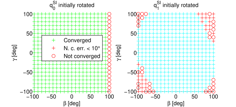
Figure 2: Simulation study: convergence behaviour ($+$: true positive (convergence detected and actually converged), $\circ$: true negative, red $+$: false negative).

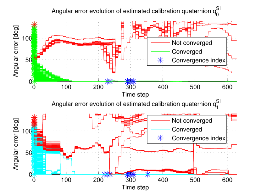
Figure 3: Simulation study: angular error evolutions. Note, in all plots, a star at time step $0$ marks the initial angular offset as calculated using Equation (17). Moreover, the two graphs show the results for the IMU, which was initialised incorrectly.

Fig. 2 provides an overview of the convergence behaviour. All initial I2S calibration-offsets are marked w.r.t. both, whether convergence was detected by the method or not (Equation (12)) and whether this detection could be considered correct or not (based on a threshold of $10^{\circ}$ mean angular error). Fig. 3 provides more detailed information about the actual angular error evolution, as well as, the time, where convergence was detected.

For the tests, where $I_{0}$ was initialised incorrectly, $420$ out of $441$ tests ($=95.24\%$) converged correctly within time step range $[227,308]$. The minimal offset angle (cf. (17)), where the test did not converge, was $100.00^{\circ}$. The maximum angle, where convergence was correctly detected, was $131.19^{\circ}$. For the tests, where $I_{1}$ was initialised incorrectly, $382$ out of $441$ tests ($=86.62\%$) converged correctly within time step range $[218,353]$. Moreover, for $28$ tests, there was no convergence detected, while both estimated I2S orientations showed a mean angular error below $10^{\circ}$ (mean taken over all time steps after $308$ for $I_{0}$ and $353$ for $I_{1}$). This could be interpreted as false negatives, considering the error ranges of established calibration methods as mention in Section I. In Fig. 3, these tests appear as red plots with a rather low angular error. The minimal offset angle, where the test did not converge, was $96.72^{\circ}$. The maximum angle, where convergence was detected, was $116.46^{\circ}$.

TABLE I: Simulation study: error statistics for all converged tests.

	$\mathbf{I_{0}}$: mean, std, max	$\mathbf{I_{1}}$: mean, std, max
Pos. error $\mathbf{I^{S}}[m]$	$0.013$, $0.014$, $0.053$	$0.008$, $0.004$, $0.024$
Abs. ang. error $\mathbf{q^{SI}}[\circ]$	$0.574$, $0.358$, $3.435$	$0.136$, $0.119$, $0.629$
Abs. ang. error $\mathbf{q^{SG}}[\circ]$	$0.575$, $0.357$, $3.442$	$0.136$, $0.119$, $0.630$

Table I provides error statistics for the estimated I2S calibrations, as well as, the segment orientations, computed from all converged tests, after the time, where convergence was detected. The average calibration errors are small, in sub-degree range for both IMUs (though comparably higher for $I_{0}$), in the order of a centimetre for $I_{0}$ and in the order of millimetres for $I_{1}$, providing overall good precision. Moreover, low standard deviations and maximum values indicate good repeatability, though the maximum values for $I_{0}$ are higher than those for $I_{1}$. Note, for $q^{SI}_{0}$, all angular errors above $2^{\circ}$ were observed with initial angular offsets of $q^{SI}_{1}$ above $90^{\circ}$, indicating a stronger error propagation from $I_{1}$ to $I_{0}$. Another interesting observation is that the mean angular errors of $q^{SI}$ are nearly identical to those of $q^{SG}$. This indicates that (a) orientation calibration errors propagate linearly into the estimated segment orientations and (b) that the tracking does not add significant errors given the otherwise perfect conditions in this simulation study.

In summary, the proposed method correctly converged from a wide range of I2S initialisations, up to above $95^{\circ}$ of angular offset for both IMUs. There were no false positive convergence detections. For $I_{1}$, there were a few false negatives.

VI-B Contribution of different model equations (case study)

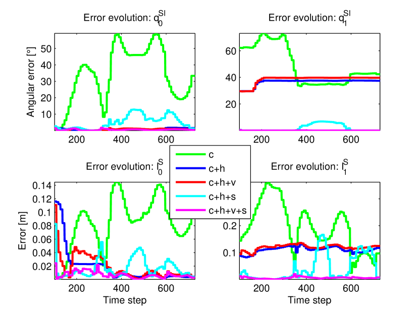
Figure 4: Simulation case study: calibration error evolutions when using different combinations of constraints, stochastic equations and priors (c=connected segments, h=hinge, v=velocity, s=shape).

As major contribution of this work we consider the combination of different constraints, stochastic equations and priors in order to sufficiently constrain the estimation problem, so that the I2S calibrations can be correctly estimated under motion from only small batches of data. Fig. 4 shows the contributions of the different constraints and priors exemplified for one representative simulation test ($\gamma=45^{\circ},\beta=-45^{\circ}$ applied to $I_{1}$). Here, it is clearly visible that only the combination of all proposed constraints and priors leads to convergence of the estimated I2S calibrations of both segments. A more in depth study under different movements and configurations is planned as future work.

VII Real data case study

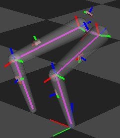
Figure 5: Real data case study: biomechanical model with capsules.

In order to test the proposed method under real conditions, IMU data and global segment poses were captured at $240$ Hz from one subject ($33$ years, $1.85$m, $77$kg) performing five squat exercises at normal speed using the Xsens MVN BIOMECH Link inertial mocap system in lower body configuration (cf. [7]). While the latter includes $7$ IMUs on feet, lower legs, upper legs and pelvis, the feet IMUs were excluded from the study, since these were stationary during recording. The segment lengths were measured and entered into the system manually and the N-pose option was used for calibration. We also measured the leg circumferences manually in order to obtain the required radii for our proposed biomechanical model, which is illustrated in Fig. 5. In summary, the setup included $5$ IMUs on right and left upper and lower legs and pelvis $\mathbb{I}=\{I_{ru},I_{rl},I_{lu},I_{ll},I_{p}\}$, mounted on a biomechanical model with $5$ segments $\mathbb{S}=\{S_{ru},S_{rl},S_{lu},S_{ll},S_{p}\}(\|p^{S}_{ru/lu}\|=0.546m,\|p^{S}_{rl/ll}\|=0.440m)$. Respective capsules $\mathbb{C}=\{C_{ru},C_{rl},C_{lu},C_{ll}\}$ ($r_{p,ru/lu}=0.074m,r_{d,ru/lu}=r_{p,rl/ll}=0.049m,r_{d,rl/ll}=0.027m$) were only modelled for the legs and the $4$ I2S calibrations for the legs were in the focus of the analysis. The hips were represented as ball-and-socket joints, while the knees were represented as hinge joints with rotation axes obtained from [23]: $\mathbb{J}=\{J_{lh},J_{rh},J_{lk},J_{rk}\}$, $\mathbb{H}=\{J_{lk},J_{rk}\},h^{S}_{lk}=[0.159,-0.979,0.124]^{T},h^{S}_{rk}=[0.152,0.951,0.138]^{T}$, RoM $=[\theta_{min,lk/rk}=0,\theta_{max,lk/rk}=162]^{\circ}$. The endpoints of the lower legs were assumed to have fixed positions during the squat movement. The target I2S calibrations were chosen as indicated in Fig. 5. In this study, a batch size $w=5$ was used to lower processing time. For our case study, the I2S rotations and segment poses, as extracted from the captured data, as well as, manually measured I2S positions (since these are not provided by the capturing system), were considered as “well established” reference values. Note, since these data cannot be considered ground truth (cf. Section I and [37]), the focus of the real data case study was on repeatability of the calibration results.

Compared to the simulation study, the real data case study shows the following additional challenges for the proposed method:

• The capsule model (cf. Fig. 5) is only a rough approximation of the subject’s body shape and the I2S poses therefore do not perfectly coincide with the shape prior.

• The IMU data is noisy and biased (note, the gyroscope bias has been approximated from a stationary sequence and subtracted in a preprocessing step).

• The knee is not a perfect hinge and the axis is estimated.

• Not all DoFs of the biomechanical model, in particular the hips, are fully excited during the squat motion.

• All I2S calibrations for the leg IMUs are simultaneously initialised incorrectly.

The ability of the proposed method to produce repeatable calibration results under these challenging conditions was tested by using three different I2S initialisation scenarios, namely:

(1) plausible: refers, for both legs, to the same initialisation as chosen in the simulation study (cf. Fig. 1).

(2) simple: refers to a default configuration, where all IMUs were initialised at the middle of the segment on the capsule surface, their local $z$- and $y$-axes being aligned with the segments’ $x$- and $y$-axes, respectively. Note, this initial configuration is consistent with the shape prior.

(3) perfect: refers to the I2S orientations obtained from the reference system via the N-pose calibration and the measured I2S positions.

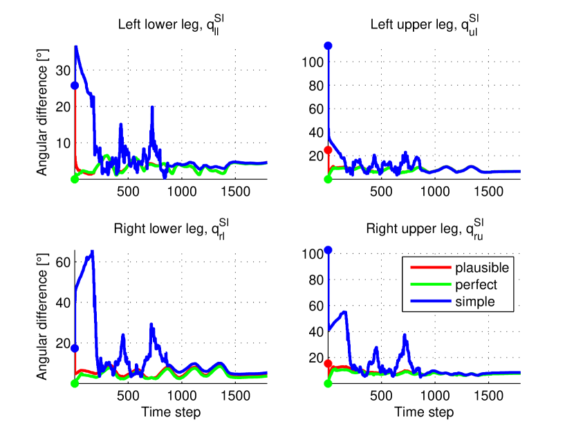
Figure 6: Real data case study: convergence of the different I2S orientations (difference w.r.t. reference).

TABLE II: Real data case study: results for three different I2S initialisations.

	Diff. to ref.: min, max		In-between diff.: min, max
	initial	final	initial	final
$\mathbf{{q^{SI}}_{ll}}[\circ]$	$0.000,\,25.73$	$4.516,\,4.613$	$0.000,\,25.73$	$0.000,\,1.178$
$\mathbf{{q^{SI}}_{lu}}[\circ]$	$0.000,\,113.6$	$6.634,\,6.664$	$24.76,\,113.6$	$0.079,\,0.417$
$\mathbf{{q^{SI}}_{rl}}[\circ]$	$0.000,\,17.36$	$3.620,\,5.295$	$0.000,\,17.36$	$0.405,\,1.707$
$\mathbf{{q^{SI}}_{ru}}[\circ]$	$0.000,\,102.8$	$7.777,\,8.451$	$15.27,\,102.8$	$0.371,\,1.287$
$\mathbf{{I^{S}}_{ll}}[m]$	$0.000,\,0.076$	$0.036,\,0.066$	$0.000,\,0.077$	$0.028,\,0.062$
$\mathbf{{I^{S}}_{lu}}[m]$	$0.000,\,0.093$	$0.080,\,0.090$	$0.055,\,0.093$	$0.004,\,0.012$
$\mathbf{{I^{S}}_{rl}}[m]$	$0.000,\,0.077$	$0.046,\,0.060$	$0.000,\,0.077$	$0.014,\,0.030$
$\mathbf{{I^{S}}_{ru}}[m]$	$0.000,\,0.092$	$0.061,\,0.067$	$0.055,\,0.092$	$0.003,\,0.006$

Table II summarizes the minimum and maximum differences of the initial and final I2S calibrations of all test configurations w.r.t. the reference values, as well as, among each other. Note, since the perfect initialisation is one of the test cases, the minimum initial differences to the reference are all zero. However, the maximal differences are above $113^{\circ}$ in orientation and $0.09m$ in position. Looking at the final calibration results, these are all reasonably close to the reference calibration, with a maximum angular difference of $8.451^{\circ}$ and a maximum position difference of $0.067m$ in the right upper leg. Recall, that the reference values cannot be considered ground truth. We also confirmed that this difference was not introduced through the shape prior, by observing that the same result was obtained when removing this prior and starting from the perfect calibration.

More importantly, all initial I2S calibrations converged to very similar final I2S orientations, with an in-between maximum angular difference of only $1.7^{\circ}$. This is a promising result, which confirms the capability of the algorithm to produce repeatable calibrations, as already indicated in the simulation study.

The maximum in-between I2S position difference was $0.062m$ for the right lower leg, which is significantly larger than for the upper legs ($0.012m$, $0.006m$). This might be explained by the low amount of motion in the lower legs as compared to the upper legs during the squat exercise, yielding less information for the calibration estimation.

Fig. 6 shows the evolutions of the I2S orientation differences w.r.t. the reference for all IMUs. The figure clearly shows the different initialisations and the convergence to similar results towards the end of the sequence. What can also be observed is a smooth but periodic change of all estimated I2S orientations during the sequence, particularly in the calibration estimate of the lower right leg and the upper left leg. This behaviour can have different sources, one of them being a time dependent I2S calibration change due to soft-tissue artefacts. Such effects will be further investigated as part of our future work.

VIII Conclusion

This paper presents a method for simultaneous I2S calibration and body motion estimation from inertial sensors mounted on the body. The method is based on sliding window constrained WLS optimisation and combines state-of-the-art motion and measurement models with different, partly novel biomechanical constraints, stochastic equations and priors. Through experiments with simulated and real data, it has been shown that the method can successfully estimate accurate and repeatable I2S calibrations from a wide range of initialisations. For simulated data, the I2S calibrations converged reliably up to $95^{\circ}$ and convergences were observed up to a maximal tested initial angular offset of $131.19^{\circ}$, where the average precision was in the order of sub-degrees for the orientation and in the order of a centimetre for the position. For real data, initialisations up to an initial angular difference of $113^{\circ}$ converged to similar results within a range of below $2^{\circ}$.

Given its online capable nature, the proposed method can not only be used for initial I2S calibration without the need for precisely executed calibration poses or motions, but it could also be used for on-the-fly re-calibration, given an appropriate detection, e.g. when an IMU slipped during recording. This would significantly improve the usability of such systems.

References

- [1] N. Miller, O. C. Jenkins, M. Kallmann, and M. J. Mataric, “Motion capture from inertial sensing for untethered humanoid teleoperation.” in Proceedings of the 4th International Conference on Humanoid Robots, November 2004.
- [2] E. Ruffaldi, L. Peppoloni, and A. Filippeschi, “Sensor fusion for complex articulated body tracking applied in rowing,” Journal of Sports Engineering and Technology, vol. 1, no. 11, 2015.
- [3] D. T.-P. Fong and Y.-Y. Chan, “The use of wearable inertial motion sensors in human lower limb biomechanics studies: a systematic review.” Sensors, vol. 10, no. 12, pp. 11 556–11 565, 2010.
- [4] G. Bleser, D. Steffen, A. Reiss, M. Weber, G. Hendeby, and L. Fradet, “Personalized physical activity monitoring using wearable sensors,” in Smart Health. Springer, February 2015, vol. 8700, pp. 99–124.
- [5] G. Bleser, D. Damen, A. Behera, G. Hendeby, K. Mura, M. Miezal, A. Gee, N. Petersen, G. Maçães, H. Domingues et al., “Cognitive learning, monitoring and assistance of industrial workflows using egocentric sensor networks,” PLOS ONE, vol. 10, no. 6, 2015.
- [6] http://www.optitrack.com/motion-capture-biomechanics/.
- [7] D. Roetenberg, H. Luinge, and P. Slycke, “Xsens MVN: Full 6DOF human motion tracking using miniature inertial sensors,” Xsens Technologies, Tech. Rep., 2013.
- [8] G. Ligorio and A. M. Sabatini, “Dealing with magnetic disturbances in human motion capture: A survey of techniques,” Micromachines, vol. 7, no. 3, 2016.
- [9] M. Miezal, G. Bleser, N. Schmitz, and D. Stricker, “A generic approach to inertial tracking of arbitrary kinematic chains,” in Proceedings of the 8th International Conference on Body Area Networks, Boston, Massachusetts, US, October 2013.
- [10] M. El-Gohary and J. McNames, “Human joint angle estimation with inertial sensors and validation with a robot arm,” Transactions on Biomedical Engineering, vol. 62, no. 7, July 2015.
- [11] F. Wenk and U. Frese, “Posture from motion,” in Proceedings of the International Conference on Intelligent Robots and Systems (IROS), Hamburg, Germany, September 2015.
- [12] M. Kok, J. Hol, and T. Schön, “An optimization-based approach to human body motion capture using inertial sensors,” in Proceedings of the 19th World Congress of the International Federation of Automatic Control (IFAC), Cape Town, South Africa, August 2014.
- [13] W. De Vries, H. Veeger, A. Cutti, C. Baten, and F. Van der Helm, “Functionally interpretable local coordinate systems for the upper extremity using inertial & magnetic measurement systems,” Journal of Biomechanics, vol. 43, no. 10, pp. 1983–1988, 2010.
- [14] E. Palermo, S. Rossi, F. Marini, F. Patanè, and P. Cappa, “Experimental evaluation of accuracy and repeatability of a novel body-to-sensor calibration procedure for inertial sensor-based gait analysis,” Measurement, vol. 52, pp. 145–155, 2014.
- [15] O. Rettig, L. Fradet, P. Kasten, P. Raiss, and S. I. Wolf, “A new kinematic model of the upper extremity based on functional joint parameter determination for shoulder and elbow,” Gait & Posture, vol. 30, no. 4, pp. 469–476, 2009.
- [16] A. G. Cutti, A. Giovanardi, L. Rocchi, A. Davalli, and R. Sacchetti, “Ambulatory measurement of shoulder and elbow kinematics through inertial and magnetic sensors.” Medical Biological Engineering and Computing, vol. 46, no. 2, pp. 169–178, 2008.
- [17] B. Bouvier, S. Duprey, L. Claudon, R. Dumas, and A. Savescu, “Upper limb kinematics using inertial and magnetic sensors: Comparison of sensor-to-segment calibrations,” Sensors, vol. 15, no. 8, pp. 813–833, 2015.
- [18] M. Kok and T. Schön, “Maximum likelihood calibration of a magnetometer using inertial sensors,” in Proceedings of the 19th World Congress of the International Federation of Automatic Control (IFAC), Cape Town, South Africa, August 2014.
- [19] J. Wahlström, I. Skog, and P. Händel, “IMU alignment for smartphone-based automotive navigation.” in Proceedings of the 18th International Conference on Information Fusion, Washington, D.C., US, July 2015.
- [20] M. Li, H. Yu, X. Zheng, A. Mourikis et al., “High-fidelity sensor modeling and self-calibration in vision-aided inertial navigation,” in Proceedings of the International Conference on Robotics and Automation (ICRA), Hong Kong, China, June 2014.
- [21] D. Cucci, M. Matteucci et al., “Position tracking and sensors self-calibration in autonomous mobile robots by Gauss-Newton optimization,” in Proceedings of the International Conference on Robotics and Automation (ICRA), Hong Kong, China, May 2014.
- [22] O. Birbach and B. Bauml, “Calibrating a pair of inertial sensors at opposite ends of an imperfect kinematic chain,” in Proceedings of the International Conference on Intelligent Robots and Systems (IROS), Chicago, Illinois, US, September 2014.
- [23] T. Seel, J. Raisch, and T. Schauer, “IMU-based joint angle measurement for gait analysis,” Sensors, vol. 14, no. 4, pp. 6891–6909, 2014.
- [24] S. Salehi, G. Bleser, A. Reiss, and D. Stricker, “Body-IMU autocalibration for inertial hip and knee joint tracking,” in Proceedings of the 10th International Conference on Body Area Networks, Sydney, Australia, September 2015.
- [25] C. V. Rao, J. B. Rawlings, and J. H. Lee, “Constrained linear state estimation a moving horizon approach,” Automatica, vol. 37, no. 10, pp. 1619–1628, Oct. 2001.
- [26] V. Zatsiorsky, Kinetics of Human Motion. Human Kinetics, 2002.
- [27] R. Trieb, A. Ballester, G. Kartsounis, S. Alemany, J. Uriel, G. Hansen, F. Fourli, M. Sanguinetti, and M. Vangenabith, “Eurofit - integration, homogenisation and extension of the scope of large 3D anthropometric data pools for product development,” in Proceedings of the 4th International Conference and Exhibition on 3D Body Scanning Technologies, Long Beach, CA, November 2013.
- [28] K. E. Peyer, M. Morris, and W. I. Sellers, “Subject-specific body segment parameter estimation using 3D photogrammetry with multiple cameras,” PeerJ, vol. 3, no. e831, 2015.
- [29] O. Wasenmüller, J. C. Peters, V. Golyanik, and D. Stricker, “Precise and automatic anthropometric measurement extraction using template registration,” in Proceedings of the International Conference on 3D Body Scanning Technologies, Lugano, Switzerland, 2015.
- [30] M. Miezal, B. Taetz, N. Schmitz, and G. Bleser, “Ambulatory inertial spinal tracking using constraints,” in Proceedings of the 9th International Conference on Body Area Networks, London, Great Britain, September 2014.
- [31] G. Bleser and D. Stricker, “Advanced tracking through efficient image processing and visual–inertial sensor fusion,” Computers & Graphics, vol. 33, no. 1, pp. 59–72, 2009.
- [32] I. Skog, P. Händel, J.-O. Nilsson, and J. Rantakokko, “Zero-velocity detection—an algorithm evaluation,” Transactions on Biomedical Engineering, vol. 57, no. 11, pp. 2657–2666, 2010.
- [33] M. D. Shuster and S. Oh, “Three-axis attitude determination from vector observations,” Journal of Guidance, Control, and Dynamics, vol. 4, no. 1, pp. 70–77, 1981.
- [34] S. Boyd and L. Vandenberghe, Convex Optimization. New York: Cambridge University Press, 2004.
- [35] K. Levenberg, “A method for the solution of certain problems in least squares.” Quaterly Journal on Applied Mathematics, no. 2, pp. 164–168, 1944.
- [36] J. Nocedal and S. J. Wright, Numerical Optimization, 2nd ed., ser. Springer series in operations research and financial engineering. New York: Springer, 2006.
- [37] J.-T. Zhang, A. C. Novak, B. Brouwer, and Q. Li, “Concurrent validation of Xsens MVN measurement of lower limb joint angular kinematics,” Physiological Measurement, vol. 34, no. 8, p. N63, 2013.