2016–157 12 June 2016

The COMPASS Collaboration The COMPASS Collaboration

Exclusive production of $\omega$ mesons was studied at the COMPASS experiment by scattering $160~{}\mathrm{GeV}/\mathit{c}$ muons off transversely polarised protons. Five single-spin and three double-spin azimuthal asymmetries were measured in the range of photon virtuality $1~{}(\mathrm{GeV}/\mathit{c})^{2}<Q^{2}<10~{}(\mathrm{GeV}/\mathit{c})^{2}$, Bjorken scaling variable $0.003<x_{\mathit{Bj}}<0.3$ and transverse momentum squared of the $\omega$ meson $0.05~{}(\mathrm{GeV}/\mathit{c})^{2}<p_{T}^{2}<0.5~{}(\mathrm{GeV}/\mathit{c})^{2}$. The measured asymmetries are sensitive to the nucleon helicity-flip Generalised Parton Distributions (GPD) $E$ that are related to the orbital angular momentum of quarks, the chiral-odd GPDs $H_{T}$ that are related to the transversity Parton Distribution Functions, and the sign of the $\pi\omega$ transition form factor. The results are compared to recent calculations of a GPD-based model.

The COMPASS Collaboration

C. Adolpherlangen, M. Aghasyantriest_i, R. Akhunzyanovdubna, M.G. Alexeevturin_u, G.D. Alexeevdubna, A. Amorosoturin_uturin_i, V. Andrieuxsaclay, N.V. Anfimovdubna, V. Anosovdubna, W. Augustyniakwarsaw, A. Austregesilomunichtu, C.D.R. Azevedoaveiro, B. Badełekwarsawu, F. Balestraturin_uturin_i, J. Barthbonnpi, R. Beckbonniskp, Y. Bedfersaclay, J. Bernhardmainzcern, K. Bickermunichtucern, E. R. Bielertcern, R. Birsatriest_i, J. Bisplinghoffbonniskp, M. Bodlakpraguecu, M. Boersaclay, P. Bordalolisbona, F. Bradamantetriest_utriest_i, C. Braunerlangen, A. Bressantriest_utriest_i, M. Büchelefreiburg, W.-C. Changtaipei, C. Chatterjeecalcutta, M. Chiossoturin_uturin_i, I. Choiillinois, S.-U. Chungmunichtub, A. Cicuttintriest_ictptriest_i, M.L. Crespotriest_ictptriest_i, Q. Curielsaclay, S. Dalla Torretriest_i, S.S. Dasguptacalcutta, S. Dasguptatriest_utriest_i, O.Yu. Denisovturin_i, L. Dharacalcutta, S.V. Donskovprotvino, N. Doshitayamagata, V. Duictriest_u, W. Dünnweberr, M. Dziewieckiwarsawtu, A. Efremovdubna, P.D. Eversheimbonniskp, W. Eyricherlangen, M. Faesslerr, A. Ferrerosaclay, M. Fingerpraguecu, M. Finger jr.praguecu, H. Fischerfreiburg, C. Francolisbon, N. du Fresne von Hoheneschemainz, J.M. Friedrichmunichtu, V. Frolovdubnacern, E. Fucheysaclay, F. Gautheronbochum, O.P. Gavrichtchoukdubna, S. Gerassimovmoscowlpimunichtu, F. Giordanoillinois, I. Gnesiturin_uturin_i, M. Gorzellikfreiburg, S. Grabmüllermunichtu, A. Grassoturin_uturin_i, M. Grosse Perdekampillinois, B. Grubemunichtu, T. Grussenmeyerfreiburg, A. Guskovdubna, F. Haasmunichtu, D. Hahnebonnpi, D. von Harrachmainz, R. Hashimotoyamagata, F.H. Heinsiusfreiburg, R. Heitzillinois, F. Herrmannfreiburg, F. Hinterbergerbonniskp, N. Horikawanagoyad, N. d’Hosesaclay, C.-Y. Hsiehtaipeix, S. Hubermunichtu, S. Ishimotoyamagatae, A. Ivanovturin_uturin_i, Yu. Ivanshindubna, T. Iwatayamagata, R. Jahnbonniskp, V. Jarypraguectu, R. Joostenbonniskp, P. Jörgfreiburg, E. Kabußmainz, B. Ketzerbonniskp,G.V. Khaustovprotvino, Yu.A. Khokhlovprotvinogv, Yu. Kisselevdubna, F. Kleinbonnpi, K. Klimaszewskiwarsaw, J.H. Koivuniemibochum, V.N. Kolosovprotvino, K. Kondoyamagata, K. Königsmannfreiburg, I. Konorovmoscowlpimunichtu, V.F. Konstantinovprotvino, A.M. Kotzinianturin_uturin_i, O.M. Kouznetsovdubna, M. Krämermunichtu, P. Kremserfreiburg, F. Krinnermunichtu, Z.V. Kroumchteindubna, Y. Kulinichillinois, F. Kunnesaclay, K. Kurekwarsaw, R.P. Kurjatawarsawtu, A.A. Lednevprotvino, A. Lehmannerlangen, M. Levillainsaclay, S. Levoratotriest_i, Y.-S. Liantaipeiy, J. Lichtenstadttelaviv, R. Longoturin_uturin_i, A. Maggioraturin_i, A. Magnonsaclay, N. Makinsillinois, N. Makketriest_utriest_i, G.K. Mallotcern, C. Marchandsaclay, B. Marianskiwarsaw, A. Martintriest_utriest_i, J. Marzecwarsawtu, J. Matoušekpraguecutriest_i, H. Matsudayamagata, T. Matsudamiyazaki, G.V. Meshcheryakovdubna, M. Meyerillinoissaclay, W. Meyerbochum, T. Michigamiyamagata, Yu.V. Mikhailovprotvino, M. Mikhasenkobonniskp, E. Mitrofanovdubna, N. Mitrofanovdubna, Y. Miyachiyamagata, P. Montuengaillinois, A. Nagaytsevdubna, F. Nerlingmainz, D. Neyretsaclay, V.I. Nikolaenkoprotvino, J. Novýpraguectucern, W.-D. Nowakmainz, G. Nukazukayamagata, A.S. Nuneslisbon, A.G. Olshevskydubna, I. Orlovdubna, M. Ostrickmainz, D. Panzieriturin_pturin_i, B. Parsamyanturin_uturin_i, S. Paulmunichtu, J.-C. Pengillinois, F. Pereiraaveiro, M. Pešekpraguecu, D.V. Peshekhonovdubna, N. Pierremainzsaclay, S. Platchkovsaclay, J. Pochodzallamainz, V.A. Polyakovprotvino, J. Pretzbonnpih, M. Quaresmalisbon, C. Quintanslisbon, S. Ramoslisbona, C. Regalifreiburg, G. Reicherzbochum, C. Riedlillinois, M. Roskotpraguecu, D.I. Ryabchikovprotvinov, A. Rybnikovdubna, A. Rychterwarsawtu, R. Salacpraguectu, V.D. Samoylenkoprotvino, A. Sandaczwarsaw, C. Santostriest_i, S. Sarkarcalcutta, I.A. Savindubna, T. Sawadataipei G. Sbrizzaitriest_utriest_i, P. Schiavontriest_utriest_i, K. Schmidtfreiburgc, H. Schmiedenbonnpi, K. Schönningcerni, S. Schopfererfreiburg, E. Sedersaclay, A. Selyunindubna, O.Yu. Shevchenkodubna, L. Silvalisbon, L. Sinhacalcutta, S. Sirtlfreiburg, M. Sluneckadubna, J. Smolikdubna, F. Sozzitriest_i, A. Srnkabrno, D. Steffencernmunichtu, M. Stolarskilisbon, M. Sulcliberec, H. Suzukiyamagatad, A. Szabelskiwarsaw, T. Szameitatfreiburgc, P. Sznajderwarsaw, S. Takekawaturin_uturin_i, M. Tasevskydubna, S. Tessarotriest_i, F. Tessarottotriest_i, F. Thibaudsaclay, F. Toselloturin_i, V. Tskhaymoscowlpi, S. Uhlmunichtu, J. Velosoaveiro, M. Viriuspraguectu, J. Vondrapraguectu, S. Wallnermunichtu, T. Weisrockmainz, M. Wilfertmainz, J. ter Wolbeekfreiburgc, K. Zarembawarsawtu, P. Zavadadubna, M. Zavertyaevmoscowlpi, E. Zemlyanichkinadubna, M. Ziembickiwarsawtu and A. Zinkerlangen

turin_pUniversity of Eastern Piedmont, 15100 Alessandria, Italy

aveiroUniversity of Aveiro, Department of Physics, 3810-193 Aveiro, Portugal

bochumUniversität Bochum, Institut für Experimentalphysik, 44780 Bochum, Germanyls

bonniskpUniversität Bonn, Helmholtz-Institut für Strahlen- und Kernphysik, 53115 Bonn, Germanyl

bonnpiUniversität Bonn, Physikalisches Institut, 53115 Bonn, Germanyl

brnoInstitute of Scientific Instruments, AS CR, 61264 Brno, Czech Republicm

calcuttaMatrivani Institute of Experimental Research & Education, Calcutta-700 030, Indian

dubnaJoint Institute for Nuclear Research, 141980 Dubna, Moscow region, Russiao

erlangenUniversität Erlangen–Nürnberg, Physikalisches Institut, 91054 Erlangen, Germanyl

freiburgUniversität Freiburg, Physikalisches Institut, 79104 Freiburg, Germanyls

cernCERN, 1211 Geneva 23, Switzerland

liberecTechnical University in Liberec, 46117 Liberec, Czech Republicm

lisbonLIP, 1000-149 Lisbon, Portugalp

mainzUniversität Mainz, Institut für Kernphysik, 55099 Mainz, Germanyl

miyazakiUniversity of Miyazaki, Miyazaki 889-2192, Japanq

moscowlpiLebedev Physical Institute, 119991 Moscow, Russia

munichtuTechnische Universität München, Physik Department, 85748 Garching, Germanylr

nagoyaNagoya University, 464 Nagoya, Japanq

praguecuCharles University in Prague, Faculty of Mathematics and Physics, 18000 Prague, Czech Republicm

praguectuCzech Technical University in Prague, 16636 Prague, Czech Republicm

protvinoState Scientific Center Institute for High Energy Physics of National Research Center ‘Kurchatov Institute’, 142281 Protvino, Russia

saclayIRFU, CEA, Université Paris-Saclay, 91191 Gif-sur-Yvette, Frances

taipeiAcademia Sinica, Institute of Physics, Taipei 11529, Taiwan

telavivTel Aviv University, School of Physics and Astronomy, 69978 Tel Aviv, Israelt

triest_uUniversity of Trieste, Department of Physics, 34127 Trieste, Italy

triest_iTrieste Section of INFN, 34127 Trieste, Italy

triest_ictpAbdus Salam ICTP, 34151 Trieste, Italy

turin_uUniversity of Turin, Department of Physics, 10125 Turin, Italy

turin_iTorino Section of INFN, 10125 Turin, Italy

illinoisUniversity of Illinois at Urbana-Champaign, Department of Physics, Urbana, IL 61801-3080, USA

warsawNational Centre for Nuclear Research, 00-681 Warsaw, Polandu

warsawuUniversity of Warsaw, Faculty of Physics, 02-093 Warsaw, Polandu

warsawtuWarsaw University of Technology, Institute of Radioelectronics, 00-665 Warsaw, Polandu

yamagataYamagata University, Yamagata 992-8510, Japanq

Deceased

aAlso at Instituto Superior Técnico, Universidade de Lisboa, Lisbon, Portugal

bAlso at Department of Physics, Pusan National University, Busan 609-735, Republic of Korea and at Physics Department, Brookhaven National Laboratory, Upton, NY 11973, USA

rSupported by the DFG cluster of excellence ‘Origin and Structure of the Universe’ (www.universe-cluster.de)

dAlso at Chubu University, Kasugai, Aichi 487-8501, Japanq

xAlso at Department of Physics, National Central University, 300 Jhongda Road, Jhongli 32001, Taiwan

eAlso at KEK, 1-1 Oho, Tsukuba, Ibaraki 305-0801, Japan

gAlso at Moscow Institute of Physics and Technology, Moscow Region, 141700, Russia

vSupported by Presidential grant NSh–999.2014.2

hPresent address: RWTH Aachen University, III. Physikalisches Institut, 52056 Aachen, Germany

yAlso at Department of Physics, National Kaohsiung Normal University, Kaohsiung County 824, Taiwan

iPresent address: Uppsala University, Box 516, 75120 Uppsala, Sweden

cSupported by the DFG Research Training Group Programme 1102 “Physics at Hadron Accelerators”

lSupported by the German Bundesministerium für Bildung und Forschung

sSupported by EU FP7 (HadronPhysics3, Grant Agreement number 283286)

mSupported by Czech Republic MEYS Grant LG13031

nSupported by SAIL (CSR), Govt. of India

oSupported by CERN-RFBR Grant 12-02-91500

pSupported by the Portuguese FCT - Fundação para a Ciência e Tecnologia, COMPETE and QREN, Grants CERN/FP 109323/2009, 116376/2010, 123600/2011 and CERN/FIS-NUC/0017/2015

qSupported by the MEXT and the JSPS under the Grants No.18002006, No.20540299 and No.18540281; Daiko Foundation and Yamada Foundation

tSupported by the Israel Academy of Sciences and Humanities

uSupported by the Polish NCN Grant 2015/18/M/ST2/00550

1 Introduction

Hard exclusive meson production (HEMP) in charged lepton scattering off nucleons plays an important role in studies of the nucleon structure in terms of its constituents, i.e. quarks and gluons. Interest in studying HEMP as well as deeply virtual Compton scattering (DVCS) has increased recently as this allows access to generalised parton distributions (GPDs) [1, 2, 3, 4, 5], which offer a comprehensive description of the partonic structure of the nucleon. In particular, GPDs provide a picture of the nucleon as an extended object [6, 7, 8]. In this picture, which is often referred to as 3-dimensional nucleon tomography, longitudinal momenta and transverse spatial degrees of freedom of partons are correlated. Constraining GPDs may also yield an insight into angular momenta of quarks, which represent another fundamental property of the nucleon [2, 3]. The mapping of nucleon GPDs, which became one of the key objectives of hadron physics, requires a comprehensive programme of measuring hard exclusive production of photons and various mesons in a broad kinematic range.

The amplitude for hard exclusive meson production by longitudinally polarised virtual photons was proven to factorise into a hard scattering part that is calculable in perturbative QCD (pQCD) and a soft part [4, 9]. The soft part contains GPDs that describe the structure of the target nucleon and a distribution amplitude (DA), which accounts for the structure of the produced meson. The factorisation holds in the limit of large photon virtuality $Q^{2}$ and large invariant mass $W$ of the virtual-photon nucleon system, but fixed $x_{\mathit{Bj}}$, and for $|t|/Q^{2}\ll 1$. Here, $t$ is the squared four-momentum transfer to the proton and $x_{\mathit{Bj}}=Q^{2}/(2M_{p}\nu)$, where $\nu$ is the energy of the virtual photon in the lab frame and $M_{p}$ is the proton mass. This factorisation is referred to as ‘collinear’ because parton transverse momenta are neglected. No similar proof of factorisation exists for transversely polarised virtual photons. However, phenomenological pQCD-inspired models have been proposed [10, 11, 12, 13] that go beyond the collinear factorisation by postulating the so called ‘$k_{\perp}$ factorisation’, where $k_{\perp}$ denotes the parton transverse momentum. In the model of Refs. [11, 12, 13, 14, 15], hereafter referred to as ‘GK’ model, cross sections and spin-density matrix elements (SDMEs) for HEMP by both longitudinal and transverse virtual photons can be described simultaneously.

At leading twist, the chiral-even GPDs $H^{f}$ and $E^{f}$, where $f$ denotes a quark of a given flavour or a gluon, are sufficient to describe exclusive vector meson production on a spin $\nicefrac{{1}}{{2}}$ target. These GPDs are of special interest as they are related to the total angular momentum carried by partons in the nucleon [2]. When higher-twist effects are included in the DA, the chiral-odd GPDs $H_{T}^{f}$ and $\overline{E}_{T}^{f}$ appear, which describe the process amplitude with helicity flip of the exchanged quark. They are also referred to as ‘transverse’ GPDs. While parameterisations of GPDs $H^{f}$ over the presently accessible $x_{\mathit{Bj}}$ range are well constrained by existing measurements of DVCS and HEMP, much less experimental results exist that allow one to constrain the other mentioned GPDs. For references to measurements relevant for constraining GPDs $H^{f}$ and $E^{f}$ see e.g. the introductory sections in Refs. [16, 17]. Depending on quark content and quantum numbers of the meson, the soft part of the process amplitude contains specific combinations of flavour-dependent quark GPDs and gluon GPDs [18, 19, 20]. Because of this property HEMP can be regarded as a quark flavour filter, which motivates the study of a wide spectrum of mesons.

The COMPASS collaboration has already published results on azimuthal asymmetries for exclusive $\rho^{0}$ production on transversely polarised protons [16, 17] and deuterons [16], which were compared with predictions of the GPD model of Refs. [13, 14]. These asymmetries are sensitive to all types of GPDs, including the chiral-odd GPDs $H_{T}$ and $\overline{E}_{T}$. In particular, the leading-twist asymmetry $A_{\mathrm{UT}}^{\sin\left(\phi-\phi_{S}\right)}$ (see Sec. 2 for the definition) is sensitive to the chiral-even GPDs $E$. These GPDs are of special interest, as they describe transitions with nucleon helicity flip and are related to the orbital angular momentum of quarks. The model describes well the COMPASS data obtained for $\rho^{0}$ and provides their interpretation in terms of GPDs. The measured asymmetry $A_{\mathrm{UT}}^{\sin\left(\phi-\phi_{S}\right)}$ is of small magnitude, because for GPDs $E$ in $\rho^{0}$ production the valence quark contribution is expected to be small. This is interpreted as approximate cancellation due to opposite signs and similar magnitudes of GPDs $E^{u}$ and $E^{d}$ for valence quarks [13]. Also, the small gluon and sea contributions evaluated in Ref. [13] cancel here to a large extent. The model also explains the non-vanishing asymmetry $A_{\mathrm{UT}}^{\sin\phi_{S}}$ by a significant contribution from chiral-odd GPDs $H_{T}$ that are related to transversity parton distribution functions. It is the first experimental indication in hard exclusive $\rho^{0}$ production of the contribution of these chiral-odd GPDs.

The interest in studying transverse spin azimuthal asymmetries in hard exclusive $\omega$ production is twofold. First, due to the different quark combinations in the flavour-dependent wave functions of the mesons, certain asymmetries are expected to be larger for $\omega$ production than the corresponding ones for $\rho^{0}$. In particular, for $A_{\mathrm{UT}}^{\sin\left(\phi-\phi_{S}\right)}$ the version of the model as described in Ref. [13] predicts a sizeable value of approximately $-0.1$ for the $\omega$ channel in contrast to a small value predicted for the $\rho^{0}$ channel. Thus the measurement of this asymmetry in both channels will provide additional constraints, which may help to separate the valence quarks contributions $E^{u}$ and $E^{d}$. Secondly, it is known since a long time that pion exchange can play an important role in photo- and leptoproduction of $\omega$ mesons [21]. The recent HERMES measurements of SDMEs for exclusive electroproduction of $\omega$ mesons [22] indicate a sizeable contribution of the unnatural-parity-exchange processes in the covered energy range. In the framework of the GK model it was shown [15] that the pion-pole exchange is important to reproduce HERMES results on SDMEs. Still, SDME data do not allow to distinguish the sign of the $\pi\omega$ transition form factor. Certain azimuthal asymmetries for $\omega$ production are sensitive to the pion-pole contribution and hence in principle could allow the determination of its sign. Although the effect of the pion-pole decreases with increasing $W$, it might still be measurable beyond experimental uncertainties at COMPASS. For other vector mesons the effect is expected to be very small ($\rho^{0}$ production) or negligible ($\phi$ production) [15].

This Paper describes the measurement of exclusive $\omega$ muoproduction on transversely polarised protons with the COMPASS apparatus. Size and kinematic dependences of azimuthal asymmetries of the cross section with respect to beam and target polarisation are determined and discussed. The related theoretical formalism is outlined in the following section. A brief presentation of the experiment is given in Sec. 3, while in Sec. 4 the data selection is reported in detail. The extraction of asymmetries and the estimation of systematic uncertainties are described in Sec. 5 and 6, respectively. Results and concluding remarks are given in Sec. 7.

2 Theoretical formalism

The cross section for exclusive $\omega$ muoproduction, $\mu\,N\to\mu^{\prime}\,\omega\,N^{\prime}$, on a transversely polarised nucleon reads [23]:

$$\left[\frac{\alpha_{\mathit{em}}}{8\pi^{3}}\frac{y^{2}}{1-\epsilon}\frac{1-x_{\mathit{Bj}}}{x_{\mathit{Bj}}}\frac{1}{Q^{2}}\right]^{-1}\frac{{\mathrm{d}}\sigma}{{\mathrm{d}}x_{\mathit{Bj}}{\mathrm{d}}Q^{2}{\mathrm{d}}t{\mathrm{d}}\phi{\mathrm{d}}\phi_{s}}=$$

$$\text{\rule{40.0pt}{0.0pt}}\text{\phantom{${}+{}$}}\frac{1}{2}\left(\sigma_{++}^{++}+\sigma_{++}^{--}\right)+\epsilon\sigma_{00}^{++}-\epsilon\cos\left(2\phi\right)\mathrm{Re}\;\sigma_{+-}^{++}$$

$$\text{\rule{40.0pt}{0.0pt}}-\sqrt{\epsilon\left(1+\epsilon\right)}\cos\phi\;\mathrm{Re}\left(\sigma_{+0}^{++}+\sigma_{+0}^{--}\right)\text{\phantom{$\Big{[}$}}$$

$$\text{\rule{40.0pt}{0.0pt}}-P_{\ell}\sqrt{\epsilon\left(1-\epsilon\right)}\sin\phi\;\mathrm{Im}\left(\sigma_{+0}^{++}+\sigma_{+0}^{--}\right)\text{\phantom{$\Big{[}$} }$$

$$\text{\rule{40.0pt}{0.0pt}}-S_{T}\text{\phantom{$P_{\ell}$}}\Big{[}\sin\left(\phi-\phi_{s}\right)\mathrm{Im}\left(\sigma_{++}^{+-}+\epsilon\sigma_{00}^{+-}\right)+\frac{\epsilon}{2}\sin\left(\phi+\phi_{s}\right)\mathrm{Im}\;\sigma_{+-}^{+-}$$

$$\text{\rule{40.0pt}{0.0pt}}\text{\phantom{$S_{T}P_{\ell}$}}+\frac{\epsilon}{2}\sin\left(3\phi-\phi_{s}\right)\mathrm{Im}\;\sigma_{+-}^{-+}+\sqrt{\epsilon\left(1+\epsilon\right)}\sin\phi_{s}\;\mathrm{Im}\;\sigma_{+0}^{+-}$$

$$\text{\rule{40.0pt}{0.0pt}}\text{\phantom{$S_{T}P_{\ell}$}}+\sqrt{\epsilon\left(1+\epsilon\right)}\sin\left(2\phi-\phi_{s}\right)\mathrm{Im}\;\sigma_{+0}^{-+}\Big{]}$$

$$\text{\rule{40.0pt}{0.0pt}}+S_{T}P_{\ell}\Big{[}\sqrt{1-\epsilon^{2}}\cos\left(\phi-\phi_{s}\right)\mathrm{Re}\;\sigma_{++}^{+-}-\sqrt{\epsilon\left(1-\epsilon\right)}\cos\phi_{s}\;\mathrm{Re}\;\sigma_{+0}^{+-}$$

$$\text{\rule{40.0pt}{0.0pt}}\text{\phantom{$S_{T}P_{\ell}$}}-\sqrt{\epsilon\left(1-\epsilon\right)}\cos\left(2\phi-\phi_{s}\right)\mathrm{Re}\;\sigma_{+0}^{-+}\Big{]},$$ (1)

where only terms relevant for the present analysis are shown. For brevity, the dependence on kinematic variables is omitted. The general formula for the cross section for meson leptoproduction can be found in Ref. [23]. The angle $\phi$ is the azimuthal angle between the lepton plane that is spanned by the momenta of the incoming and the scattered leptons, and the hadron plane that is spanned by the momenta of the virtual photon and the meson (see Fig. 1). The angle $\phi_{s}$ is the azimuthal angle between the lepton plane and the spin direction of the target nucleon.

The polarisation of the lepton beam is denoted by $P_{\ell}$. The component of the transverse target spin perpendicular to the virtual-photon direction, $S_{T}$, is approximated in the COMPASS kinematic region by the corresponding component perpendicular to the direction of the incoming muon, $P_{T}$. According to Ref. [23], the transition from $S_{T}$ to $P_{T}$ introduces in Eq. (1) a dependence on $\theta$, which is the angle between the directions of virtual photon and incoming beam particle. This dependence gives rise to additional asymmetries of the cross section that are related to longitudinal target polarisation. These asymmetries are suppressed by the factor $\sin\theta$, which is small at COMPASS kinematics ($\sin\theta\approx 0.056$ on average). In the present analysis the effect of the angle $\theta$ is neglected.

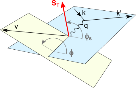
Figure 1: Kinematics of exclusive meson production in the target rest frame. Here $\mathbf{k}$, $\mathbf{k^{\prime}}$, $\mathbf{q}$ and $\mathbf{v}$ represent the three-momentum vectors of the incident and the scattered muons, the virtual photon and the meson respectively. The component of the target spin vector $\mathbf{S}$ (not shown) perpendicular to the virtual-photon direction is denoted by $\mathbf{S_{T}}$.

In the considered kinematics, where the mass of the incoming lepton $m_{\mu}\ll Q^{2}$, the virtual-photon polarisation parameter $\epsilon$ can be approximated in the following way:

$$\epsilon\approx\frac{\displaystyle 1-y-\frac{1}{4}y^{2}\gamma^{2}}{\displaystyle 1-y+\frac{1}{2}y^{2}+\frac{1}{4}y^{2}\gamma^{2}}.$$ (2)

Here, $y$ is the fractional energy of the virtual photon (see Table 1), $\gamma^{2}=\left(2x_{\mathit{Bj}}M_{p}\right)^{2}/Q^{2}$ and $M_{p}$ is the mass of the proton.

The photoabsorption cross sections or interference terms $\sigma_{ij}^{mn}$ are proportional to bilinear combinations of helicity amplitudes $\mathcal{M}$ for the photoproduction subprocess,

$$\sigma_{ij}^{mn}\propto\sum\mathcal{M}_{i^{\prime}m^{\prime},im}^{*}\mathcal{M}_{i^{\prime}m^{\prime},jn},$$ (3)

where the helicity of the virtual photon is denoted by $i,j=-1,0,+1$ and the helicity of the initial-state proton is denoted by $m,n=-\nicefrac{{1}}{{2}},+\nicefrac{{1}}{{2}}$. The sum runs over all combinations of helicities of meson ($i^{\prime}=-1,0,+1$) and final-state proton ($m^{\prime}=-\nicefrac{{1}}{{2}},+\nicefrac{{1}}{{2}}$). In the following the helicities $-1,-\nicefrac{{1}}{{2}},0,+\nicefrac{{1}}{{2}},+1$ will be labelled by only their sign or zero, omitting $\nicefrac{{1}}{{2}}$ or $1$.

For a transversely polarised target five single ($\mathrm{UT}$) and three double ($\mathrm{LT}$) spin asymmetries can be defined:

$$A_{\mathrm{UT}}^{\sin\left(\phi-\phi_{s}\right)\text{\phantom{$3$}}} =-\frac{\mathrm{Im}\left(\sigma_{++}^{+-}+\epsilon\sigma_{00}^{+-}\right)}{\sigma_{0}}, A_{\mathrm{LT}}^{\cos\left(\phi-\phi_{s}\right)\text{\phantom{$3$}}} =\phantom{-}\frac{\mathrm{Re}\;\sigma_{++}^{+-}}{\sigma_{0}},$$

$$A_{\mathrm{UT}}^{\sin\left(\phi+\phi_{s}\right)\text{\phantom{$3$}}} =-\frac{\mathrm{Im}\;\sigma_{+-}^{+-}}{\sigma_{0}}, A_{\mathrm{LT}}^{\cos\phi_{s}\text{\phantom{$\left(3\phi+\right)$}}} =-\frac{\mathrm{Re}\;\sigma_{+0}^{+-}}{\sigma_{0}},$$

$$A_{\mathrm{UT}}^{\sin\left(3\phi-\phi_{s}\right)} =-\frac{\mathrm{Im}\;\sigma_{+-}^{-+}}{\sigma_{0}}, A_{\mathrm{LT}}^{\cos\left(2\phi-\phi_{s}\right)} =-\frac{\mathrm{Re}\;\sigma_{+0}^{-+}}{\sigma_{0}},$$

$$A_{\mathrm{UT}}^{\sin\phi_{s}\text{\phantom{$\left(3\phi+\right)$}}} =-\frac{\mathrm{Im}\;\sigma_{+0}^{+-}}{\sigma_{0}},$$

$$A_{\mathrm{UT}}^{\sin\left(2\phi-\phi_{s}\right)} =-\frac{\mathrm{Im}\;\sigma_{+0}^{-+}}{\sigma_{0}}.$$ (4)

Here, $\sigma_{0}$ is the total unpolarised cross section, which is the sum of the cross sections for longitudinally and transversely polarised virtual photons, $\sigma_{L}$ and $\sigma_{T}$, respectively:

$$\sigma_{0}=\frac{1}{2}\left(\sigma_{++}^{++}+\sigma_{++}^{--}\right)+\epsilon\sigma_{00}^{++}=\sigma_{T}+\epsilon\sigma_{L}.$$ (5)

Each asymmetry is related to a modulation of the cross section as a function of $\phi$ and/or $\phi_{s}$ (see Eq. (1)), which is indicated by the superscript.

Calculations for the full set of five $A_{\mathrm{UT}}$ and three $A_{\mathrm{LT}}$ asymmetries were performed recently in the framework of the GK model [14]. Of particular interest for an interpretation of the COMPASS results described in this Paper are three asymmetries, which can be expressed through helicity amplitudes neglecting terms containing unnatural parity exchange amplitudes:

$$\sigma_{0}\;A_{\mathrm{UT}}^{\sin\left(\phi-\phi_{s}\right)\text{\phantom{$3$}}} =-2\mathrm{Im}\left[\epsilon\mathcal{M}_{0-,0+}^{*}\mathcal{M}_{0+,0+}+\mathcal{M}_{+-,++}^{*}\mathcal{M}_{++,++}+\tfrac{1}{2}\mathcal{M}_{0-,++}^{*}\mathcal{M}_{0+,++}\right]~{},$$

$$\sigma_{0}\;A_{\mathrm{UT}}^{\sin\left(2\phi-\phi_{s}\right)} =-\phantom{2}\mathrm{Im}\left[\mathcal{M}_{0+,++}^{*}\mathcal{M}_{0-,0+}\right]~{},$$

$$\sigma_{0}\;A_{\mathrm{UT}}^{\sin\phi_{s}\text{\phantom{$\left(3\phi+\right)$}}} =-\phantom{2}\mathrm{Im}\left[\mathcal{M}_{0-,++}^{*}\mathcal{M}_{0+,0+}-\mathcal{M}_{0+,++}^{*}\mathcal{M}_{0-,0+}\right]~{}.$$ (6)

Most of the neglected amplitudes are related to pion pole exchange, the role of which will be discussed in Sec. 7.

The dominant contribution from the $\gamma^{*}_{L}\rightarrow V_{L}$ transition, where $V$ denotes vector meson, is described by $\mathcal{M}_{0+,0+}$ and $\mathcal{M}_{0-,0+}$, which are related to chiral-even GPDs $H$ and $E$. The suppressed contribution from the $\gamma^{*}_{T}\rightarrow V_{T}$ transition is described by $\mathcal{M}_{++,++}$ and $\mathcal{M}_{+-,++}$, which are also related to chiral-even GPDs. A description of the $\gamma^{*}_{T}\rightarrow V_{L}$ transition is possible by including chiral-odd GPDs $H_{T}$ and $\overline{E}_{T}$, which are related to $\mathcal{M}_{0-,++}$ and $\mathcal{M}_{0+,++}$, respectively. The $\gamma^{*}_{L}\rightarrow V_{T}$ and $\gamma^{*}_{T}\rightarrow V_{-T}$ transitions are known to be suppressed and are neglected here.

Different values are predicted for the asymmetry $A_{\mathrm{UT}}^{\sin\left(\phi-\phi_{S}\right)}$ in $\rho^{0}$ and $\omega$ productions, as already mentioned above. For this asymmetry, the contribution of chiral-odd GPDs is expected to be negligible, as one can see for instance from the comparison of calculations for the $\rho^{0}$ channel in Refs. [13] and [14]. The asymmetry $A_{\mathrm{UT}}^{\sin\phi_{S}}$ represents an imaginary part of two bilinear products of helicity amplitudes. The first product is related to GPDs $H$ and $H_{T}$, while the second one is related to GPDs $E$ and $\overline{E}_{T}$. The latter product appears also in the asymmetry $A_{\mathrm{UT}}^{\sin\left(2\phi-\phi_{S}\right)}$. For the $\rho^{0}$ channel the asymmetry $A_{\mathrm{UT}}^{\sin\phi_{S}}$ was found to be different from zero, while the asymmetry $A_{\mathrm{UT}}^{\sin\left(2\phi-\phi_{S}\right)}$ is compatible with zero [17]. This implies a non-negligible contribution of GPDs $H_{T}$ in this case.

A summary of the kinematic variables used in this Paper is given in Table 1.

Table 1: Kinematic variables.

$k$	four-momentum of incident muon
$k^{\prime}$	four-momentum of scattered muon
$p$	four-momentum of target nucleon
$v$	four-momentum of $\omega$ meson
$q=k-k^{\prime}$	four-momentum of virtual photon
$Q^{2}=-q^{2}$	negative invariant mass squared of virtual photon
$W=\sqrt{(p+q)^{2}}$	invariant mass of the $\gamma^{*}-N$ system
$M_{p}$	proton mass
$\nu=(p\cdot q)/M_{p}$	energy of virtual photon in the laboratory system
$x_{\mathit{Bj}}=Q^{2}/(2M_{p}\nu)$	Bjorken scaling variable
$y=(p\cdot q)/(p\cdot k)$	fraction of lepton energy lost in the laboratory system
$M_{\pi\pi\pi}$	invariant mass of $\pi^{+}\pi^{-}\pi^{0}$ system
$t=(q-v)^{2}$	square of the four-momentum transfer to the target nucleon
$p_{T}^{2}$	transverse momentum squared of vector meson with
	respect to the virtual-photon direction
$E_{\omega}$	energy of $\omega$ in the laboratory system
$M_{X}^{2}=(p+q-v)^{2}$	missing mass squared of the undetected system
$E_{\textrm{miss}}=((p+q-v)^{2}-p^{2})/(2M_{p})$	missing energy of the undetected system
$\phantom{E_{\textrm{miss}}}=({M_{X}^{2}-M_{p}^{2}})/({2M_{p}})$
$\phantom{E_{\textrm{miss}}}=\nu-E_{\omega}+t/(2M_{p})$

3 Experimental set-up

COMPASS is a fixed-target experiment situated at the high-intensity M2 beam line of the CERN SPS. A detailed description of the experiment can be found in Ref. [24].

The $\mu^{+}$ beam had a nominal momentum of $160~{}\mathrm{GeV}/\mathit{c}$ with a spread of $5\%$ and a longitudinal polarisation of $P_{\ell}\approx-0.8$ known with the precision of $5\%$. The data were taken at a mean intensity of $3.5\times 10^{8}~{}\mu/\mathrm{spill}$, for a spill length of about $10~{}\mathrm{s}$ every $40~{}\mathrm{s}$. A measurement of the trajectory and the momentum of each incoming muon is performed upstream of the target. The momentum of the beam muon is measured with a relative precision better than $1\%$.

The beam traverses a solid-state ammonia ($\mathrm{NH}_{3}$) target that contains transversely polarised protons. The target is situated within a large aperture magnet with a dipole holding field of $0.5~{}\mathrm{T}$. The $2.5~{}\mathrm{T}$ solenoidal field is only used when polarising the target material. A mixture of liquid ${}^{3}\mathrm{He}$ and ${}^{4}\mathrm{He}$ is used to cool the target to $50~{}\mathrm{mK}$. Ten nuclear magnetic resonance (NMR) coils surrounding the target allow for a determination of the target polarisation $P_{T}$, which typically amounts to $0.8$ with an uncertainty of $3\%$. The ammonia is contained in three cylindrical target cells with a diameter of $4~{}\mathrm{cm}$, placed along the beam with $5~{}\mathrm{cm}$ space between cells. The central cell is $60~{}\mathrm{cm}$ long and the two outer ones are $30~{}\mathrm{cm}$ long. The spin directions in neighbouring cells are opposite. Such a target configuration allows for a simultaneous measurement of azimuthal asymmetries for the two target spin directions without relying on beam flux measurements. Systematic effects due to acceptance are reduced by reversing the spin directions on a weekly basis. With the three-cell configuration, the average acceptance for cells with opposite spin direction is approximately the same, which leads to a further reduction of systematic uncertainties.

The dilution factor $f$, which is the cross-section-weighted fraction of polarisable material, is calculated for incoherent exclusive $\omega$ production using the measured material composition and the nuclear dependence of the cross section:

$$f=\frac{n_{p}}{n_{p}+\sum_{A}{n_{A}\frac{\widetilde{\sigma}_{A}}{\sigma_{p}}}}.$$ (7)

Here, $n_{p}$ and $n_{A}$ denote the numbers of polarisable protons in the target and of unpolarised nucleons in the target material with atomic mass $A$, respectively. The sum runs over all nuclei present in the COMPASS target. The ratio of the cross section per nucleon for a given nucleus to the cross section on the proton is denoted by $\widetilde{\sigma}_{A}/\sigma_{p}$. The inclusion of the effect of nuclear shadowing on the calculation of the dilution factor is crucial for the ammonia target. However, this effect has never been measured for exclusive $\omega$ production in a kinematic region comparable to that covered by the COMPASS experiment. Therefore, we assume that the nuclear shadowing effect for $\omega$ is the same as that for $\rho^{0}$. This assumption is supported by similar quark compositions, quantum numbers ($J^{P}$) and masses of both mesons. The assumption leads to the same dilution factor as for $\rho^{0}$, the evaluation of which is detailed in Ref. [25]. For the $\mathrm{NH}_{3}$ target, which is used for the present analysis, the dilution factor amounts typically to $0.25$ [16].

The COMPASS spectrometer is designed to reconstruct scattered muons and produced hadrons in wide momentum and angular ranges. It consists of two stages, each equipped with a dipole magnet, to measure tracks with large and small momenta, respectively. In the high-flux region, in or close to the beam, tracking is provided by stations of scintillating fibres, silicon detectors, micromesh gaseous chambers and gas electron multiplier chambers. Large-angle tracking devices are multiwire proportional chambers, drift chambers and straw detectors. Muons are identified in large-area mini drift tubes and drift tubes placed downstream of hadron absorbers. Each stage of the spectrometer contains an electromagnetic and a hadron calorimeter. The identification of charged particles is possible with a RICH detector, although in this analysis it is not used.

The data recording system is activated by several triggers. For inclusive triggers, the scattered muon is identified by a coincidence of signals from trigger hodoscopes. Semi-inclusive triggers select events with a scattered muon and an energy deposit in a hadron calorimeter exceeding a given threshold. Moreover, a pure calorimeter trigger with a high energy threshold was implemented to extend the acceptance towards high $Q^{2}$ and large $x_{\mathit{Bj}}$. It was checked that this trigger does not introduce any bias due to the acceptance of the calorimeters in the $x_{\mathit{Bj}}$ range covered by the present data. Veto counters upstream of the target are used to suppress beam halo muons.

4 Event sample

The results presented in this Paper are based on the data taken with the transversely polarised $\mathrm{NH}_{3}$ target in 2010. An event to be accepted for further analysis is required to have the same topology as that of the observed process

Therefore, we select only events that have an incident muon track, a scattered muon track, exactly two additional tracks of oppositely charged hadrons, which are all associated to a vertex in the polarised target material, and a single $\pi^{0}$ meson that is reconstructed using its two decay photons detected in the electromagnetic calorimeters.

The flux of the incoming beam is equalised for all target cells using appropriate cuts on position and angle of beam tracks. Figure 2 shows the distribution of the reconstructed vertex position $z_{V}$ along the beam axis. In this figure as well as in Figs. 3 to 7, the distributions are obtained applying all selections except that corresponding to the displayed variable.

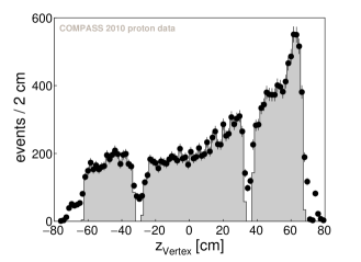
Figure 2: Distribution of z-coordinate of reconstructed primary vertices. The accepted events are denoted by the shaded area.

In order to obtain a data sample in the deep inelastic scattering region, the following kinematic cuts are applied: $1~{}(\mathrm{GeV}/\mathit{c})^{2}<Q^{2}<10~{}(\mathrm{GeV}/\mathit{c})^{2}$, where the lower cut selects the perturbative QCD region and the upper one is chosen to remove the region of $Q^{2}$ where the fraction of non-exclusive background is large; $0.1<y<0.9$, in order to suppress radiative corrections (large $y$) or poorly reconstructed kinematics (low $y$). The latter cut removes also events from the region of hadron resonances at small values of $W$. A small residual number of such events is removed by requiring $W$ to be larger than $5~{}\mathrm{GeV}/\mathit{c}^{2}$.

4.1 Reconstruction of $\pi^{0}$

A neutral pion is reconstructed using clusters in the electromagnetic calorimeters (ECALs), which are required not to be associated to charged particle tracks. Only events with two such clusters, which have to pass the selections described below, are retained for the analysis. The possibility to reconstruct $\pi^{0}$ mesons by using events with more than two clusters and examining all cluster combinations was checked in Ref. [26]. As such combinatorial method would lead to an increase of background by more than a factor of two, it is not applied in this analysis.

A photon reconstructed in a given ECAL is accepted only if its energy $E_{\gamma}$ is in the range

$$0.6~{}\mathrm{GeV}<E_{\gamma}<25~{}\mathrm{GeV}~{}~{}~{}\mathrm{for~{}ECAL1},$$

$$1.0~{}\mathrm{GeV}<E_{\gamma}<50~{}\mathrm{GeV}~{}~{}~{}\mathrm{for~{}ECAL2}.$$ (8)

Here, ECAL1 (ECAL2) denotes the electromagnetic calorimeter in the large (small) angle stage of the spectrometer. The yields of exclusive $\omega$ mesons were studied as a function of the values of the lower limits on $E_{\gamma}$ resulting in maximal yields for the indicated values. The purity of the exclusive $\omega$ sample only weakly depends on these lower limits. The upper limits on $E_{\gamma}$ are determined by requiring sufficient statistics needed for a reliable determination of the $E_{\gamma}$-dependent parameterisation of the time correlation between a given decay photon candidate and the incoming muon track. In order to ensure this correlation, the difference of the measured ECAL cluster time and the measured time of the incoming muon, $\Delta t=t_{\gamma}-t_{\mu}$, is calculated. Since the precision of time reconstruction in ECALs depends on the cluster energy, the time correlation is ensured by requiring

$$|\Delta t-\Delta t_{\mathrm{par}}(E_{\gamma})|<3~{}\sigma_{\mathrm{par}}(E_{\gamma})~{}.$$ (9)

For each calorimeter, position $\Delta t_{\mathrm{par}}(E_{\gamma})$ and width $\sigma_{\mathrm{par}}(E_{\gamma})$ of the $\gamma-\mu$ correlation peak are parameterised as a function of $E_{\gamma}$ using a sample of events for semi-inclusive $\pi^{0}$ production.

Similarly, the limit on the invariant mass of two photons, $M_{\gamma\gamma}$, depends on the energy $E_{\gamma\gamma}$ of the $\pi^{0}$ candidate:

$$|M_{\gamma\gamma}-M_{\pi^{0},\;\mathrm{par}}(E_{\gamma\gamma})|<3~{}\sigma_{\mathrm{par}}(E_{\gamma\gamma})~{}.$$ (10)

Also here, position $M_{\pi^{0},\;\mathrm{par}}(E_{\gamma\gamma})$ and width $\sigma_{\mathrm{par}}(E_{\gamma\gamma})$ of the $\pi^{0}$ peak are parameterised using semi-inclusive data for $\pi^{0}$ mesons reconstructed in each of the three possible combinations of neutral clusters in ECALs. In addition to the real data, similar parameterisations are obtained also for Monte Carlo data that are used for the procedure of background subtraction, see Sec. 5. The parameterisations are obtained in the following ranges of energy:

$$1.2~{}\mathrm{GeV} <E_{\gamma\gamma}<25~{}\mathrm{GeV}~{}~{}~{}\mathrm{for~{}ECAL1},$$

$$2.0~{}\mathrm{GeV} <E_{\gamma\gamma}<50~{}\mathrm{GeV}~{}~{}~{}\mathrm{for~{}ECAL2},$$

$$1.6~{}\mathrm{GeV} <E_{\gamma\gamma}<35~{}\mathrm{GeV}~{}~{}~{}\mathrm{for~{}ECAL1+ECAL2}.$$ (11)

The selection of $\pi^{0}$ mesons is restricted to the ranges of energy given in Eq. (11). The distribution of $M_{\gamma\gamma}$ for reconstructed events is shown in Fig. 3, where the accepted events are represented by the shaded histogram. Note that there are no sharp limits on this histogram, because the energy-dependent selection on $M_{\gamma\gamma}$ is applied, see Eq. (10).

Figure 3: Distribution of the invariant mass of two photons. The accepted events are denoted by the shaded area.

In order to reduce the smearing related to ECAL reconstruction, after having performed the $\pi^{0}$ selection the energies of decay photons for each event are rescaled by the factor

$$f_{E_{\gamma}}=\frac{M_{\pi^{0}}^{\mathrm{PDG}}}{M_{\gamma\gamma}},$$ (12)

where $M_{\pi^{0}}^{\mathrm{PDG}}\approx 0.135~{}\mathrm{GeV}/\mathit{c}^{2}$ is the nominal $\pi^{0}$ mass. This reduces the width $\sigma_{\omega}$ of the reconstructed $\omega$ resonance from $25~{}\mathrm{MeV}/\mathit{c}^{2}$ to $20~{}\mathrm{MeV}/\mathit{c}^{2}$.

4.2 Selection of incoherent exclusive $\omega$ production

Events corresponding to incoherent exclusive $\omega$ production are selected using additional cuts on:

• the invariant mass of the $\pi^{+}\pi^{-}\pi^{0}$ system, $M_{\pi^{+}\pi^{-}\pi^{0}}$,

  $$\left|M_{\pi^{+}\pi^{-}\pi^{0}}-M_{\omega}^{\mathrm{PDG}}\right|<60~{}\mathrm{MeV}/\mathit{c}^{2},$$ (13)

  where $M_{\omega}^{\mathrm{PDG}}=782.65~{}\mathrm{MeV}/\mathit{c}^{2}$ is the nominal $\omega$ resonance mass;
  

• the missing energy $E_{\mathrm{miss}}$,

  $$-3.0~{}\mathrm{GeV}<E_{\textrm{miss}}<3.0~{}\mathrm{GeV};$$ (14)

• the $\omega$ meson energy in the laboratory system,

  $$E_{\omega}>14~{}\mathrm{GeV};$$ (15)

• the transverse momentum squared of the $\omega$ meson with respect to the virtual-photon direction,

  $$0.05~{}(\mathrm{GeV}/\mathit{c})^{2}<p_{T}^{2}<0.5~{}(\mathrm{GeV}/\mathit{c})^{2}.$$ (16)

The $\omega$ meson is reconstructed using two charged hadrons and a reconstructed $\pi^{0}$. As RICH information is not used in this analysis, the charged pion mass hypothesis is assigned to each hadron track. Figure 4 shows the corresponding invariant mass spectrum that indicates clearly the $\omega$ signal at the nominal position, $M_{\omega}^{\mathrm{PDG}}=782.65~{}\mathrm{MeV}/\mathit{c}^{2}$. The selection of $\omega$ mesons using the invariant mass range given by Eq. (13) corresponds to the $\pm 3\sigma_{\omega}$ region around $M_{\omega}^{\mathrm{PDG}}$.

Figure 4: Distribution of $M_{\pi^{+}\pi^{-}\pi^{0}}$. The accepted events are denoted by the shaded area.

Figure 5: Distribution of $E_{\mathrm{miss}}$. The accepted events are denoted by the shaded area.

As the recoiling proton is not detected, exclusive events are selected by the cut on missing energy given by Eq. (14). The selected range is referred to as ‘signal region’ in the following. The distribution of $E_{\mathrm{miss}}$ is shown in Fig. 5, where the exclusive peak at $E_{\mathrm{miss}}\approx 0$ is clearly visible. The boundaries of the $E_{\mathrm{miss}}$ range for the selection of exclusive events are chosen to cover the $\pm 2\sigma$ region of the exclusive peak. Since it is not possible to distinguish on an event-by-event basis between signal and background events in the signal window, the background asymmetries are probed in the second range of $E_{\mathrm{miss}}$,

$$7~{}\mathrm{GeV}<E_{\mathrm{miss}}<20~{}\mathrm{GeV},$$ (17)

where only semi-inclusive background events contribute. The intermediate range, $3~{}\mathrm{GeV}<E_{\mathrm{miss}}<7~{}\mathrm{GeV}$, is contaminated by diffractive-dissociation events ($\gamma^{*}N\rightarrow\omega N^{*}$, where $N^{*}\rightarrow N+\pi+\ldots$), as indicated by results of Monte Carlo simulations [27, 28]. Similarly as in the $\rho^{0}$ analysis [17], this range is not taken into account in the present analysis. In order to reduce further the semi-inclusive background contribution, events are accepted only if the energy of the $\omega$ meson in the laboratory system is large enough, see Eq. (15).

Diffractive dissociation background in the exclusive sample is examined using a Monte Carlo event generator called HEPGEN [27]. Using both exclusive and nucleon-dissociative $\omega$ events generated by HEPGEN, which are reconstructed and selected as the real data, the contribution from low-mass diffractive dissociation of the nucleon, corresponding to the $E_{\mathrm{miss}}$ range given in Eq. (14), is found to be $\approx 14\%$ of the exclusive $\omega$ signal.

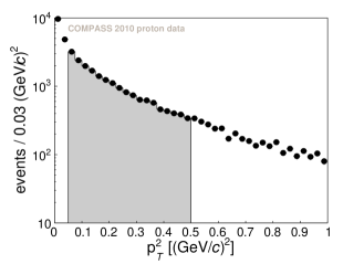
Figure 6: Distribution of $p_{T}^{2}$. The accepted events are denoted by the shaded area.

The $p_{T}^{2}$ distribution is shown in Fig. 6. We choose to use $p_{T}^{2}$ rather than $t$ or $t^{\prime}=|t|-t_{0}$, where $t_{0}$ is the minimal kinematically allowed $|t|$. The reason is that in the COMPASS kinematic region and for the set-up without detection of the recoil particle, $p_{T}^{2}$ is determined with a precision better by a factor of two to five. In addition, the $t^{\prime}$ distribution is distorted because $t_{0}$, which depends on $W$, $Q^{2}$, $M_{\pi^{+}\pi^{-}\pi^{0}}$ and $M_{X}^{2}$, is poorly determined for non-exclusive background events [29]. The $p_{T}^{2}$ distribution shown in Fig. 6 indicates at small $p_{T}^{2}$ values a contribution from coherent $\omega$ production on target nuclei. Coherent events are suppressed by applying the lower limit given by Eq. (16). A study of $p_{T}^{2}$ distributions shows that in addition to exclusive coherent and incoherent $\omega$ production a third component, which originates from non-exclusive background, is also present and its contribution increases with $p_{T}^{2}$, thus requiring also an upper limit. Therefore, in order to select the sample of events from incoherent exclusive $\omega$ production, the afore mentioned $p_{T}^{2}$ limits are applied.

After all selections, the final sample for incoherent exclusive $\omega$ production consists of about $18500$ events. The mean values of the kinematic variables $Q^{2}$, $x_{\mathit{Bj}}$, $y$, $W$ and $p_{T}^{2}$ are given in Table 2.

Table 2: Mean values of selected kinematic variables for events reconstructed in the signal region $-3~{}\mathrm{GeV}<E_{\mathrm{miss}}<3~{}\mathrm{GeV}$ with and without the correction for semi-inclusive background [30].

	$\langle Q^{2}\rangle$ $[(\mathrm{GeV}/\mathit{c})^{2}]$	$\langle x_{\mathit{Bj}}\rangle$	$\langle y\rangle$	$\langle W\rangle$ $[\mathrm{GeV}/\mathit{c}^{2}]$	$\langle p_{T}^{2}\rangle$ $[(\mathrm{GeV}/\mathit{c})^{2}]$
signal only	2.2	0.049	0.18	7.1	0.17
signal + background	2.4	0.055	0.17	6.9	0.19

5 Extraction of asymmetries

The azimuthal asymmetries listed in Eq. (4) are evaluated by fitting simultaneously the exclusive signal events (denoted by subscript $\mathrm{S}$) and semi-inclusive background events (denoted by subscript $\mathrm{B}$) using the unbinned maximum likelihood estimator. This method of extraction allows us to study correlations between asymmetries and to reduce the statistical uncertainty of the measurement compared to binned estimators.

Four subsamples of events are fitted simultaneously as a function of the azimuthal angles and the missing energy. Each subsample corresponds to the specific target cell $t$ with the polarisation state $p$. Here, $t=\mathrm{C}$ and $t=\mathrm{U+D}$ refer to the central cell and the sum of upstream and downstream cells, respectively, while the two target polarisation states are denoted by $p=\uparrow$ and $p=\downarrow$. The fitted function describes the observed sum of exclusive signal and semi-inclusive background events denoted in the following by the subscript $\mathrm{S}+\mathrm{B}$:

$$N_{t,\;\mathrm{S+B}}^{p}(\phi,\phi_{s},E_{\mathrm{miss}})=c_{t,\;\mathrm{S}+\mathrm{B}}^{p}(\phi,\phi_{s},E_{\mathrm{miss}})~{}g_{t,\;\mathrm{S+B}}^{p}(\phi,\phi_{s},E_{\mathrm{miss}}).$$ (18)

In the factor

$$c_{t,\;\mathrm{S}+\mathrm{B}}^{p}(\phi,\phi_{s},E_{\mathrm{miss}})=F~{}n~{}\left[\sigma_{0,\;\mathrm{S}}^{\phantom{p}}~{}a_{t,\;\mathrm{S}}^{p}(\phi,\phi_{s},E_{\mathrm{miss}})+\sigma_{0,\;\mathrm{B}}^{\phantom{p}}~{}a_{t,\;\mathrm{B}}^{p}(\phi,\phi_{s},E_{\mathrm{miss}})\right]$$ (19)

$F$ is the muon flux, $n$ is the number of target nucleons, $\sigma_{0,\;\mathrm{S}(\mathrm{B})}^{\phantom{p}}$ are the spin-averaged cross sections and $a_{t,\;\mathrm{S}(\mathrm{B})}^{p}(\phi,\phi_{s},E_{\mathrm{miss}})$ are the acceptances for cell $t$ with polarisation $p$, where $\mathrm{S}(\mathrm{B})$ denotes either $\mathrm{S}$ or $\mathrm{B}$. The factor

$$g_{t,\;\mathrm{S+B}}^{p}(\phi,\phi_{s},E_{\mathrm{miss}})=1\pm\gamma_{t,\;\mathrm{S}}^{p}(\phi,\phi_{s},E_{\mathrm{miss}})~{}A_{\mathrm{raw},\;\mathrm{S}}(\phi,\phi_{s})\pm\gamma_{t,\;\mathrm{B}}^{p}(\phi,\phi_{s},E_{\mathrm{miss}})~{}A_{\mathrm{raw},\;\mathrm{B}}(\phi,\phi_{s})$$ (20)

describes the measured azimuthal modulations of the cross section for longitudinally polarised beam and transversely polarised target. In Eq. (20),

$$\gamma_{t,\;\mathrm{S}(\mathrm{B})}^{p}(\phi,\phi_{s},E_{\mathrm{miss}})=\frac{\sigma_{0,\;\mathrm{S}(\mathrm{B})}^{\phantom{p}}~{}a_{t,\;\mathrm{S}(\mathrm{B})}^{p}(\phi,\phi_{s},E_{\mathrm{miss}})}{\sigma_{0,\;\mathrm{S}}^{\phantom{p}}~{}a_{t,\;\mathrm{S}}^{p}(\phi,\phi_{s},E_{\mathrm{miss}})+\sigma_{0,\;\mathrm{B}}^{\phantom{p}}~{}a_{t,\;\mathrm{B}}^{p}(\phi,\phi_{s},E_{\mathrm{miss}})}$$ (21)

are the weights corresponding to the fractions of signal and background processes that are evaluated from the data as described in the following, while

$$A_{\mathrm{raw},\;\mathrm{S}(\mathrm{B})}(\phi,\phi_{s}) =A_{\mathrm{raw},\;\mathrm{S}(\mathrm{B})}^{\sin\left(\phi-\phi_{s}\right)}\sin\left(\phi-\phi_{s}\right)+A_{\mathrm{raw},\;\mathrm{S}(\mathrm{B})}^{\sin\left(\phi+\phi_{s}\right)}\sin\left(\phi+\phi_{s}\right)+A_{\mathrm{raw},\;\mathrm{S}(\mathrm{B})}^{\sin\left(2\phi-\phi_{s}\right)}\sin\left(2\phi-\phi_{s}\right)$$

$$+A_{\mathrm{raw},\;\mathrm{S}(\mathrm{B})}^{\sin\left(3\phi-\phi_{s}\right)}\sin\left(3\phi-\phi_{s}\right)+A_{\mathrm{raw},\;\mathrm{S}(\mathrm{B})}^{\sin\phi_{s}}\sin\phi_{s}+A_{\mathrm{raw},\;\mathrm{S}(\mathrm{B})}^{\cos\left(\phi-\phi_{s}\right)}\cos\left(\phi-\phi_{s}\right)$$

$$+A_{\mathrm{raw},\;\mathrm{S}(\mathrm{B})}^{\cos\left(2\phi-\phi_{s}\right)}\cos\left(2\phi-\phi_{s}\right)+A_{\mathrm{raw},\;\mathrm{S}(\mathrm{B})}^{\cos\phi_{s}}\cos\phi_{s}$$ (22)

are the raw asymmetries that enter Eq. (20) with the sign corresponding to the target polarisation state, $+$ and $-$ for $\uparrow$ and $\downarrow$, respectively. The raw asymmetries are related to the physics asymmetries, in particular to those defined in Eq. (4) for the exclusive signal events, in the following way:

$$A_{\mathrm{UT},\;\mathrm{S}(\mathrm{B})}^{\mathrm{mod}} =\frac{A_{\mathrm{raw},\;\mathrm{S}(\mathrm{B})}^{\mathrm{mod}}}{f_{\mathrm{S}(\mathrm{B})}~{}P_{T}~{}D^{\mathrm{mod}}},$$

$$A_{\mathrm{LT},\;\mathrm{S}(\mathrm{B})}^{\mathrm{mod}} =\frac{A_{\mathrm{raw},\;\mathrm{S}(\mathrm{B})}^{\mathrm{mod}}}{f_{\mathrm{S}(\mathrm{B})}~{}P_{T}~{}P_{\ell}~{}D^{\mathrm{mod}}}.$$ (23)

Here, the first line describes $\mathrm{UT}$ and the second one $\mathrm{LT}$ asymmetries, where ‘$\mathrm{mod}$’ denotes the corresponding azimuthal modulation and $f_{\mathrm{S}(\mathrm{B})}$ is the dilution factor defined in Eq. (7). The target and beam polarisations are given by $P_{T}$ and $P_{\ell}$, respectively. The depolarisation factors $D^{\mathrm{mod}}$ depend on the virtual-photon polarisation parameter, see Eq. (2):

$$D^{\sin\left(\phi-\phi_{S}\right)\text{\phantom{$3$}}} =1~{},$$

$$D^{\sin\left(\phi+\phi_{S}\right)\text{\phantom{$3$}}} =D^{\sin\left(3\phi-\phi_{S}\right)}=\frac{\epsilon}{2}~{},$$

$$D^{\sin\left(2\phi-\phi_{S}\right)} =D^{\sin\phi_{S}}=\sqrt{\epsilon\left(1+\epsilon\right)}~{},$$

$$D^{\cos\left(\phi-\phi_{S}\right)\text{\phantom{$3$}}} =\sqrt{1-\epsilon^{2}}~{},$$

$$D^{\cos\left(2\phi-\phi_{S}\right)} =D^{\cos\phi_{S}}=\sqrt{\epsilon\left(1-\epsilon\right)}.$$ (24)

In the fit of the function given by Eq. (18), the unknowns are four functions $c_{t,\;\mathrm{S}+\mathrm{B}}^{p}(\phi,\phi_{s},E_{\mathrm{miss}})$ and sixteen physics asymmetries encoded in $g_{t,\;\mathrm{S+B}}^{p}(\phi,\phi_{s},E_{\mathrm{miss}})$. The other parameters, i.e. $\gamma_{t,\;\mathrm{S}(\mathrm{B})}^{p}$, $f_{\mathrm{S}(\mathrm{B})}$, $P_{\ell}$ and $D^{\mathrm{mod}}$, are calculated for each event, while $P_{T}$ is known from the target polarisation measurement.

Equations (18) to (22) are based upon two approximations: i) the background asymmetries do not depend on the missing energy and ii) the smearing of azimuthal angles is neglected. Approximation i) is justified by results of a study that revealed no dependence on $E_{\mathrm{miss}}$ for asymmetries in the range $7~{}\mathrm{GeV}<E_{\mathrm{miss}}<20~{}\mathrm{GeV}$, where only background events contribute. This observation agrees with our previous analyses of exclusive $\rho^{0}$ production [16, 17], where an analogous test was performed with a much better statistical precision. A possible bias on the extraction of asymmetries related to approximation ii) is estimated in Sec. 6.

When fitting Eq. (18), one has to separate the functions $c_{t,\;\mathrm{S}+\mathrm{B}}^{p}(\phi,\phi_{s},E_{\mathrm{miss}})$ and $g_{t,\;\mathrm{S+B}}^{p}(\phi,\phi_{s},E_{\mathrm{miss}})$ as due to the unknown acceptance both functions may be correlated. The separation between both functions is achieved by using the reasonable assumption that the ratio of acceptances in the cells stays the same before and after target polarisation reversal:

$$\frac{a_{\mathrm{U}+\mathrm{D},\;\mathrm{S}(\mathrm{B})}^{\uparrow}(\phi,\phi_{s},E_{\mathrm{miss}})}{a_{\mathrm{C},\;\mathrm{S}(\mathrm{B})}^{\downarrow}(\phi,\phi_{s},E_{\mathrm{miss}})}=\frac{a_{\mathrm{U}+\mathrm{D},\;\mathrm{S}(\mathrm{B})}^{\downarrow}(\phi,\phi_{s},E_{\mathrm{miss}})}{a_{\mathrm{C},\;\mathrm{S}(\mathrm{B})}^{\uparrow}(\phi,\phi_{s},E_{\mathrm{miss}})}.$$ (25)

If this assumption does not hold, false asymmetries may appear. Such a possibility is examined in Sec. 6.

Using different assumed functional forms of $c_{t,\;\mathrm{S}+\mathrm{B}}^{p}(\phi,\phi_{s},E_{\mathrm{miss}})$ in the fit has no significant effect on the fitted parameters of the function $g_{t,\;\mathrm{S+B}}^{p}(\phi,\phi_{s},E_{\mathrm{miss}})$, i.e. on the physics asymmetries. Therefore, a constant term is used in this analysis for the simplicity.

The possible dependence of $\gamma_{t,\;\mathrm{S}}^{p}(\phi,\phi_{s},E_{\mathrm{miss}})$ and $\gamma_{t,\;\mathrm{B}}^{p}(\phi,\phi_{s},E_{\mathrm{miss}})$ on the azimuthal angles is examined by using a Monte Carlo (MC) simulation of the COMPASS apparatus. In this simulation the signal and background processes were generated by HEPGEN [27] and LEPTO [31] generators, respectively. For the latter one the COMPASS tuning [32] of the JETSET parameters was used. The weights $\gamma_{t,\;\mathrm{S}}^{p}(\phi,\phi_{s},E_{\mathrm{miss}})$ and $\gamma_{t,\;\mathrm{B}}^{p}(\phi,\phi_{s},E_{\mathrm{miss}})$ are found to be independent on the azimuthal angles.

The weights $\gamma_{t,\;\mathrm{S}}^{p}(E_{\mathrm{miss}})$ and $\gamma_{t,\;\mathrm{B}}^{p}(E_{\mathrm{miss}})=1-\gamma_{t,\;\mathrm{S}}^{p}(E_{\mathrm{miss}})$ are calculated by parameterising the missing energy distribution obtained for each target cell and each target polarisation state, as illustrated in Fig. 7. In these parameterisations a Gaussian function is used for the shape of the distribution of signal events, while for background events the shape is fixed by the aforementioned MC simulation with LEPTO. In analogy to our previous analyses [16, 17], the agreement between data and MC events is improved by weighting each $E_{\mathrm{miss}}$ bin $i$ of the MC distribution by the ratio

$$w_{i}=\frac{N_{i,\;\mathrm{data}}^{\pi^{+}\pi^{+}\pi^{0}}+N_{i,\;\mathrm{data}}^{\pi^{-}\pi^{-}\pi^{0}}}{N_{i,\;\mathrm{MC}}^{\pi^{+}\pi^{+}\pi^{0}}+N_{i,\;\mathrm{MC}}^{\pi^{-}\pi^{-}\pi^{0}}}.$$ (26)

Here, $N_{i,\;\mathrm{data}}^{\pi^{\pm}\pi^{\pm}\pi^{0}}$ and $N_{i,\;\mathrm{MC}}^{\pi^{\pm}\pi^{\pm}\pi^{0}}$ are the numbers of events observed in bin $i$ for experimental data and MC, respectively, when two hadrons with the same charge are required in the selection of events. Such selection excludes any exclusive production, so that the weights for semi-inclusive events can be calculated at any value of $E_{\mathrm{miss}}$.

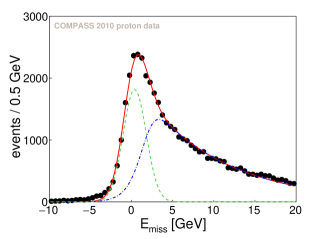
Figure 7: Parameterised distribution of $E_{\mathrm{miss}}$ for the whole data sample. The dashed (green) and dash-dotted (blue) curves represent the signal and background contributions, respectively. The sum of both contributions is represented by the solid (red) curve.

6 Systematic studies

In order to estimate the systematic uncertainties of this measurement the following contributions were examined: i) false asymmetries, ii) a possible bias of the applied estimator of the asymmetries, iii) the sensitivity to the background parameterisation, iv) the stability of asymmetries over data taking time, v) the compatibility between the three mean asymmetries obtained by averaging the one-dimensional distributions in $Q^{2}$, $x_{\mathit{Bj}}$ and $p_{T}^{2}$, vi) the uncertainty in the calculation of dilution factor, beam and target polarisations.

i) False asymmetries are extracted by analysing subsamples of data with the same spin orientation of target protons. In such a case, non-zero values of azimuthal asymmetries would indicate an experimental bias. In particular, false asymmetries provide a test of validity of the reasonable assumption, see Eq. (25), i.e. whether during data taking the acceptance has changed in a way that influences the extraction of asymmetries. False asymmetries are determined in two ways: by using the data from the upstream and downstream cells, as well as by the artificial division of the central cell into two $30~{}\mathrm{cm}$ subcells. This test is performed without separation into signal and background asymmetries, and independently for the ranges $|E_{\mathrm{miss}}|<3~{}\mathrm{GeV}$ and $-3~{}\mathrm{GeV}<E_{\mathrm{miss}}<20~{}\mathrm{GeV}$. The resulting false asymmetries are found to be consistent with zero within statistical uncertainties. Nevertheless, an upper limit on the false asymmetries is estimated to be $0.01$ [26] at the level of raw asymmetries defined in Eq. (23). This estimate represents a conservative limit for breaking the reasonable assumption given by Eq. (25). At the level of physics asymmetries, this estimation yields typically a systematic uncertainty on the level of $20\%$ of the statistical one.

ii) The check of the extraction method is twofold. First, the effect of smearing and acceptance on the extraction of asymmetries is examined by introducing an asymmetry of known value to the MC data generated with the HEPGEN generator [27], which is followed by the simulation of the COMPASS apparatus and event reconstruction. It is checked whether the unbinned maximum likelihood estimator returns the introduced asymmetry correctly. In addition, a possible mixing between asymmetries is investigated, i.e. it is checked whether a non-zero asymmetry contributes to any other asymmetry. The test shows only an effect of smearing. The related systematic uncertainty is estimated to be up to $33\%$ of the statistical one.

In the second test the obtained asymmetries are compared with those extracted with an alternative estimator that is chosen to be the 2D binned maximum likelihood estimator. In this case, in contrast to that of the unbinned estimator, the extraction of asymmetries proceeds after performing the subtraction of semi-inclusive background that is probed in the range $7~{}\mathrm{GeV}<E_{\mathrm{miss}}<20~{}\mathrm{GeV}$. This way of extraction was used in the COMPASS analysis of transverse target spin asymmetries for the $\rho^{0}$ meson [17]. The comparison indicates a good agreement between both estimators.

iii) The systematic uncertainty related to the background treatment, see Sec. 5, is estimated by assuming that the fractions of signal and background processes are known with an uncertainty of $10\%$. This assumption is supported by the COMPASS analysis for the $\rho^{0}$ meson [17], where the MC samples produced with LEPTO [31] and PYTHIA [28] generators were compared. The estimation yields typically a systematic uncertainty of $30\%$ of the statistical one.

iv) The data stability over time is examined by comparing asymmetries extracted from two consecutive subsets of data taking. A division into a larger number of subsets is not possible due to limited statistics. All asymmetries extracted from the two subsets of data are found to be compatible within statistical uncertainties.

v) The extraction of asymmetries may be unstable due to limited statistics. The effect is examined by comparing the asymmetries extracted from the entire data sample with those obtained from averaging the results obtained in bins of kinematic variables $Q^{2}$, $x_{\mathit{Bj}}$ or $p_{T}^{2}$, which are used for the extraction of final results, see Fig. 8 (right). The comparison indicates a bias that is estimated to be up to $20\%$ of the statistical uncertainty.

vi) In order to estimate the normalisation (scale) systematic uncertainty, we take into account the relative uncertainty of the target dilution factor, $2\%$, the target polarisation, $3\%$, and the beam polarisation, $5\%$. Combined in quadrature, this yields an overall systematic normalisation uncertainty of $3.6\%$ for the single-spin asymmetries and $6.2\%$ for the double-spin ones.

The systematic uncertainties for the average asymmetries obtained in i) - v) are summarised in Table 3. The total systematic uncertainties evaluated by summing in quadrature the values obtained in i) - vi) are given in Table 4.

Table 3: Systematic uncertainties for the average asymmetries obtained from the studies explained in the text. The uncertainties related to iv) are negligible for all asymmetries. The scaling uncertainties are not included in this table.

	i)	ii)	iii)	v)			i)	ii)	iii)	v)
$A_{\mathrm{UT}}^{\sin\left(\phi-\phi_{S}\right)}$	0.015	0.002	0.025	0.012		$A_{\mathrm{LT}}^{\cos\left(\phi-\phi_{S}\right)}$	0.077	0.001	0.126	0.109
$A_{\mathrm{UT}}^{\sin\left(\phi+\phi_{S}\right)}$	0.029	0.001	0.048	0.021		$A_{\mathrm{LT}}^{\cos\left(2\phi-\phi_{S}\right)}$	0.114	0.002	0.181	0.108
$A_{\mathrm{UT}}^{\sin\left(2\phi-\phi_{S}\right)}$	0.011	0.010	0.027	0.006		$A_{\mathrm{LT}}^{\cos\phi_{S}}$	0.115	0.076	0.179	0.123
$A_{\mathrm{UT}}^{\sin\left(3\phi-\phi_{S}\right)}$	0.029	0.049	0.051	0.003
$A_{\mathrm{UT}}^{\sin\phi_{S}}$	0.010	0.015	0.019	0.010

Table 4: Average azimuthal asymmetries for exclusive $\omega$ muoproduction with statistical and systematic uncertainties for all measured modulations.

	$\mathrm{A}$	$\sigma_{\mathrm{stat}}$	$\sigma_{\mathrm{sys}}$			$\mathrm{A}$	$\sigma_{\mathrm{stat}}$	$\sigma_{\mathrm{sys}}$
$A_{\mathrm{UT}}^{\sin\left(\phi-\phi_{S}\right)}$	$-0.059$	0.074	0.031		$A_{\mathrm{LT}}^{\cos\left(\phi-\phi_{S}\right)}$	$0.07$	0.42	0.18
$A_{\mathrm{UT}}^{\sin\left(\phi+\phi_{S}\right)}$	$0.06$	0.15	0.06		$A_{\mathrm{LT}}^{\cos\left(2\phi-\phi_{S}\right)}$	$0.01$	0.61	0.24
$A_{\mathrm{UT}}^{\sin\left(2\phi-\phi_{S}\right)}$	$-0.054$	0.053	0.031		$A_{\mathrm{LT}}^{\cos\phi_{S}}$	$0.54$	0.58	0.26
$A_{\mathrm{UT}}^{\sin\left(3\phi-\phi_{S}\right)}$	$0.13$	0.15	0.08
$A_{\mathrm{UT}}^{\sin\phi_{S}}$	0.096	0.059	0.028

7 Results and discussion

The measured azimuthal asymmetries, averaged over the entire kinematic range, are given in Table 4 and shown in Fig. 8 (left). In addition, the single-spin asymmetries are measured in bins of $Q^{2}$, $x_{\mathit{Bj}}$ or $p_{T}^{2}$ with the results shown in Fig. 8 (right). The double-spin asymmetries are not presented in separate kinematic bins because of large uncertainties. All published results are available in the Durham data base [33].

In Figure 8 (right) the COMPASS results are compared to the calculations of the GK model [15]. The latter are obtained for the average $W$, $Q^{2}$ and $p_{T}^{2}$ values of the COMPASS data: $W=7.1~{}\mathrm{GeV}/\mathit{c}^{2}$ and $p_{T}^{2}=0.17~{}(\mathrm{GeV}/\mathit{c})^{2}$ for the $x_{\mathit{Bj}}$ and $Q^{2}$ dependences, and $W=7.1~{}\mathrm{GeV}/\mathit{c}^{2}$ and $Q^{2}=2.2~{}(\mathrm{GeV}/c)^{2}$ for the $p_{T}^{2}$ dependence. The predictions are given for three versions of the model: with the pion-pole contribution using a positive or negative $\pi\omega$ transition form factor, and without the pion-pole contribution.

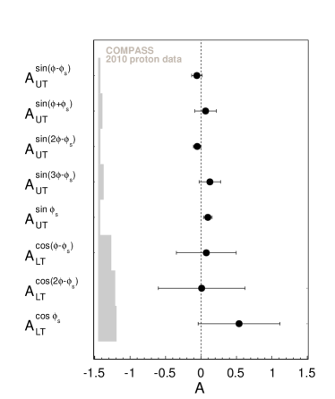
Figure 8: Left: Average azimuthal asymmetries for exclusive $\omega$ muoproduction. The error bars (left bands) represent the statistical (systematic) uncertainties. Right: Single spin azimuthal asymmetries as a function of $Q^{2}$, $x_{\mathit{Bj}}$ and $p_{T}^{2}$. The curves show the predictions of the GPD-based model [15] for the average $Q^{2}$, $W$ and $p_{T}^{2}$ values of the COMPASS data. The dashed red and dotted blue curves represent the predictions with the positive and negative $\pi\omega$ form factors, respectively, while the solid black curve represents the predictions without the pion pole.

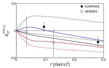
Figure 9: The asymmetry $A_{\mathrm{UT}}^{\sin\left(\phi-\phi_{S}\right)}$ for exclusive $\omega$ muoproduction measured by the COMPASS (filled circles) and HERMES [34] (open squares) collaborations as a function of $t^{\prime}$. The curves show the predictions of the GPD-based model [15] given for the average $Q^{2}$ and $W$ values of the COMPASS (solid lines) and HERMES (dashed lines) data. For each set of curves, the upper (blue) and lower (red) ones are for the negative and positive $\pi\omega$ form factors, respectively, while the middle (black) one represents the predictions without the pion pole.

The asymmetry $A_{\mathrm{UT}}^{\sin\left(\phi-\phi_{S}\right)}$ for exclusive $\omega$ production predicted by the model without pion-pole contribution is $-0.11$. This value is significantly different from that for exclusive $\rho^{0}$ production, which amounts to $-0.01$. Thus in principle a combined analysis of results for this asymmetry for both mesons could allow for a separation of the contributions of GPDs $E^{u}$ and $E^{d}$, which are different in both cases, as mentioned in the Introduction.

However, the interpretation of $\omega$ results in the context of the GPD formalism is more challenging than that for $\rho^{0}$, as exclusive $\omega$ meson production is significantly influenced by the pion-pole exchange contribution, and at present the sign of $\pi\omega$ transition form factor is unknown. By comparing the COMPASS results with the calculations of the GK model (see Fig. 8 (right)), one finds that the asymmetries $A_{\mathrm{UT}}^{\sin\left(\phi-\phi_{S}\right)}$ and $A_{\mathrm{UT}}^{\sin\left(2\phi-\phi_{S}\right)}$ prefer the negative $\pi\omega$ transition form factor, while the asymmetry $A_{\mathrm{UT}}^{\sin\phi_{S}}$ prefers the positive one. The other measured asymmetries are not sensitive to the sign of the $\pi\omega$ form factor.

The single-spin azimuthal asymmetries for $\omega$ production on transversely polarised protons were measured also by the HERMES collaboration [34]. They conclude that these data seem to favour the positive $\pi\omega$ form factor, although within large experimental uncertainties. A direct comparison of published asymmetry values measured in both experiments in not straightforward, because the HERMES definition of physics asymmetries differs from that given in Eq. (4). Such comparison is only possible for the asymmetry $A_{\mathrm{UT}}^{\sin\left(\phi-\phi_{S}\right)}$. The results from both experiments are shown as a function of $t^{\prime}$ in Fig. 9 indicating their compatibility within experimental uncertainties. Note that the COMPASS results cover a wider kinematic range and they have smaller uncertainties, for example for the asymmetry $A_{\mathrm{UT}}^{\sin\left(\phi-\phi_{S}\right)}$ by a factor larger than two.

The next measurement of exclusive meson production on a transversely polarised target is expected to be performed at Jefferson Lab after the $12~{}\mathrm{GeV}$ upgrade [35]. The foreseen data, although to be taken at different kinematics, may contribute to the determination of the sign of the $\pi\omega$ transition form factor. There are also plans to measure hard exclusive meson production on transversely polarised protons by combining a transversely polarised target with a recoil proton detector using an upgraded COMPASS set-up [36].

8 Acknowledgements

We gratefully acknowledge the support of the CERN management and staff and the skill and effort of the technicians of our collaborating institutes. This work was made possible by the financial support of our funding agencies. Special thanks go to S. V. Goloskokov and P. Kroll for providing us with the full set of model calculations as well as for the fruitful collaboration and many discussions on the interpretation of the results.

References

- [1] D. Mueller, D. Robaschik, B. Geyer, F. M. Dittes, and J. Horejsi, Wave functions, evolution equations and evolution kernels from light ray operators of QCD, Fortsch. Phys. 42, 101–141, (1994).
- [2] X.-D. Ji, Gauge-invariant decomposition of nucleon spin, Phys. Rev. Lett. 78, 610–613, (1997).
- [3] X.-D. Ji, Deeply virtual Compton scattering, Phys. Rev. D55, 7114–7125, (1997).
- [4] A. V. Radyushkin, Asymmetric gluon distributions and hard diffractive electroproduction, Phys. Lett. B385, 333–342, (1996).
- [5] A. V. Radyushkin, Nonforward parton distributions, Phys. Rev. D56, 5524–5557, (1997).
- [6] M. Burkardt, Impact parameter dependent parton distributions and off forward parton distributions for , Phys. Rev. D62, 071503, (2000). [Erratum-ibid.: D66, 119903 (2002)].
- [7] M. Burkardt, Impact parameter space interpretation for generalized parton distributions, Int. J. Mod. Phys. A18, 173–208, (2003).
- [8] M. Burkardt, Generalized parton distributions for large , Phys. Lett. B595, 245–249, (2004).
- [9] J. C. Collins, L. Frankfurt, and M. Strikman, Factorization for hard exclusive electroproduction of mesons in QCD, Phys. Rev. D56, 2982–3006, (1997).
- [10] A. D. Martin, M. G. Ryskin, and T. Teubner, The QCD description of diffractive meson electroproduction, Phys. Rev. D55, 4329–4337, (1997).
- [11] S. V. Goloskokov and P. Kroll, Vector meson electroproduction at small Bjorken- and generalized parton distributions, Eur. Phys. J. C42, 281–301, (2005).
- [12] S. V. Goloskokov and P. Kroll, The role of the quark and gluon GPDs in hard vector-meson electroproduction, Eur. Phys. J. C53, 367–384, (2008).
- [13] S. V. Goloskokov and P. Kroll, The target asymmetry in hard vector-meson electroproduction and parton angular momenta, Eur. Phys. J. C59, 809–819, (2009).
- [14] S. V. Goloskokov and P. Kroll, Transversity in exclusive vector-meson leptoproduction, Eur. Phys. J. C74, 2725, (2014). and private communication.
- [15] S. V. Goloskokov and P. Kroll, The pion pole in hard exclusive vector-meson leptoproduction, Eur. Phys. J. A50(9), 146, (2014). and private communication.
- [16] C. Adolph et al., Exclusive muoproduction on transversely polarised protons and deuterons, Nucl. Phys. B865, 1–20, (2012).
- [17] C. Adolph et al., Transverse target spin asymmetries in exclusive muoproduction, Phys. Lett. B731, 19–26, (2014).
- [18] M. Diehl, Generalized parton distributions, Phys. Rep. 388, 41–277, (2003).
- [19] M. Diehl and A. V. Vinnikov, Quarks vs. gluons in exclusive electroproduction, Phys. Lett. B609, 286–290, (2005).
- [20] S. V. Goloskokov and P. Kroll, The Longitudinal cross-section of vector meson electroproduction, Eur. Phys. J. C50, 829–842, (2007).
- [21] T. H. Bauer, R. D. Spital, D. R. Yennie, and F. M. Pipkin, The hadronic properties of the photon in high-energy interactions, Rev. Mod. Phys. 50, 261, (1978). [Erratum-ibid.: 51, 407 (1979)].
- [22] A. Airapetian et al., Spin density matrix elements in exclusive electroproduction on 1H and 2H targets at GeV beam energy, Eur. Phys. J. C74(11), 3110, (2014).
- [23] M. Diehl and S. Sapeta, On the analysis of lepton scattering on longitudinally or transversely polarized protons, Eur. Phys. J. C41, 515–533, (2005).
- [24] P. Abbon et al., The COMPASS experiment at CERN, Nucl. Instrum. Meth. A577, 455–518, (2007).
- [25] V. Yu. Alexakhin et al., Double spin asymmetry in exclusive muoproduction at COMPASS, Eur. Phys. J. C52, 255–265, (2007).
- [26] J. ter Wolbeek. Azimuthal asymmetries in hard exclusive meson muoproduction off transversely polarized protons. PhD thesis, Albert-Ludwigs-Universität, Freiburg, (2015).
- [27] A. Sandacz and P. Sznajder, HEPGEN - generator for hard exclusive leptoproduction. (2012).
- [28] T. Sjostrand, S. Mrenna, and P. Z. Skands, PYTHIA 6.4 Physics and Manual, JHEP. 05, 026, (2006).
- [29] P. Amaudruz et al., Transverse momentum distributions for exclusive muoproduction, Z. Phys. C54, 239–246, (1992).
- [30] P. Sznajder. Study of azimuthal asymmetries in exclusive leptoproduction of vector mesons on transversely polarised protons and deuterons. PhD thesis, National Centre for Nuclear Research, Warsaw, (2015).
- [31] G. Ingelman, A. Edin, and J. Rathsman, LEPTO 6.5: A Monte Carlo generator for deep inelastic lepton - nucleon scattering, Comput. Phys. Commun. 101, 108–134, (1997).
- [32] C. Adolph et al., Leading order determination of the gluon polarisation from DIS events with high- hadron pairs, Phys. Lett. B718, 922–930, (2013).
- [33] The Durham HepData Project. http://hepdata.cedar.ac.uk.
- [34] A. Airapetian et al., Transverse-target-spin asymmetry in exclusive -meson electroproduction, Eur. Phys. J. C75, 600, (2015).
- [35] J. Dudek et al., Physics Opportunities with the 12 GeV Upgrade at Jefferson Lab, Eur. Phys. J. A48, 187, (2012).
- [36] F. Gautheron et al. COMPASS-II Proposal. Technical Report CERN-SPSC-2010-014. SPSC-P-340, CERN, Geneva (May, 2010).