Segmentation of scanning electron microscopy images from natural rubber samples with gold nanoparticles using starlet wavelets

Abstract

Electronic microscopy has been used for morphology evaluation of different materials structures. However, microscopy results may be affected by several factors. Image processing methods can be used to correct and improve the quality of these results. In this paper we propose an algorithm based on starlets to perform the segmentation of scanning electron microscopy images. An application is presented in order to locate gold nanoparticles in natural rubber membranes. In this application, our method showed accuracy greater than 85% for all test images. Results given by this method will be used in future studies, to computationally estimate the density distribution of gold nanoparticles in natural rubber samples and to predict reduction kinetics of gold nanoparticles at different time periods.

Keywords: Image Processing, Gold Nanoparticles, Natural Rubber, Scanning Electron Microscopy, Segmentation, Wavelets

1 Introduction

Recently, electronic microscopy has been widely used for morphology evaluation of different materials’ micro and nanostructures, e.g. natural rubber/gold nanoparticles membranes[1], spray layer-by-layer films[2], anisotropic metal structures[3], Langmuir-Blodgett monolayers[4], among others. However, microscopy results may be affected by factors such as equipment configuration, image resolution, external conditions, such as noise level and power grid stability, and even the analyzed material, which can present surface degradation depending on the energy level of the applied electron beam.

Images obtained by electronic microscopy do not often present good quality, especially when evaluated at nanoscale structural levels, where the parameters discussed above become even more influential. Image processing methods can be used when the image is not suitable for analysis, or when the characterization needs to be automated. Digital image processing is a powerful and well-established set of techniques, such as filtering, restoration, reconstruction, object recognition and segmentation. This last processing method separates an image into its constituent objects[5], recognizing a certain region of interest.

1.1 Related work

Image segmentation is often used in microscopy images that are currently segmented to obtain features such as number of cells[6], separation of overlapped particles[7] and skull-stripping of mouse brain [8].

There are a number of commercial and free software available for these processing [9]; however, these tools are focused on some images, and cannot be extended to analysis of other ones [9, 10]. Furthermore, segmentation of nontrivial images is one of the most challenging tasks in image processing: its accuracy determines the success of computational analysis procedures [5].

1.2 Proposed approach

In this paper we propose an algorithm based on starlets to perform the segmentation of scanning electron microscopy images. This algorithm is applied in order to segment gold nanoparticles incorporated on natural rubber membranes (NR/Au). Starlets are isotropic undecimated wavelet transforms, well adapted to astronomical data, where objects present isotropy in most cases [11]. The proposed approach consists of applying the starlet transform in a sample image to obtain its detail decomposition levels. These levels are used to identify and separate background elements and noise from interest regions displayed on the input image.

Natural rubber samples were obtained from Hevea brasiliensis latex (RRIM 600 clones) by casting method, and gold nanoparticles were added by in situ chemical reduction. These samples were used for chemistry analysis and ultrasensitive detection by Raman spectroscopy in the construction of flexible SERS and SERRS substrates[12], and also in the study of the NR/Au influence on the physiology of Leishmania braziliensis protozoans [13]. Results presented in this study will be used as basis for the prediction of kinetics of gold nanoparticles reduced at different time periods in samples of natural rubber, and also in the density distribution study of gold nanoparticles in natural rubber.

The remainder of the paper is organized as follows. Section 2 introduces a brief background on starlet wavelets, the main tool of this method, and an overview of the proposed algorithm. Section 3 presents the image dataset used to test the algorithms, as well as the evaluation method to test the algorithm performance. Next, Section 4 exhibits the experimental results from algorithm application on elements of the image dataset. Also, we discuss the performance of the method. Finally, in Section 5 we report our final considerations about this study.

2 Formulation

2.1 Background on starlet transform

Starlet is an undecimated (or redundant) wavelet transform based on the algorithm “à trous” (with holes) from Holschneider[14] and Shensa [15]. This wavelet is well suited to analyze astronomical[11, 16] or biological[17] images, that usually contain isotropic objects.

Two-dimensional starlet transform is constructed from scale ($\phi$) and wavelet ($\psi$) functions[16] (Fig. 1), given on Eqs. 1 and 2:

$$\phi_{1D}(t)=\frac{1}{12}(|t-2|^{3}-4|t-1|^{3}+6|t|^{3}-4|t+1|^{3}+|t+2|^{3})$$

$$\phi(x,y)=\phi_{1D}(x)\phi_{1D}(y)$$ (1)

$$\frac{1}{4}\psi(\frac{x}{2},\frac{y}{2})=\phi(x,y)-\frac{1}{4}\phi(\frac{x}{2},\frac{y}{2})$$ (2)

where $\phi_{1D}$ is the one-dimensional B-spline of order 3 (B3-spline). Starck and Murtagh[11, 16, 18] used extensively the B3-spline as $\phi$, by its attributes: it is a smooth function, adequate to the isolation of larger structures in an image, and supports separability, allowing fast computation.

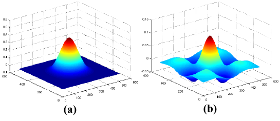
Figure 1: 2D starlet transform. (a) Two-dimensional scale function, $\phi$. (b) Two-dimensional wavelet, $\psi$.

The pair of filters $(h,g)$ related to this wavelet is[16]:

$$h_{1D}[k]=[\begin{array}[]{ccccc}1&4&6&4&1\end{array}]/16,k=-2,...2$$ (4)

$$h[k,l]=h_{1D}[k]h_{1D}[l]$$ (5)

$$g[k,l]=\delta[k,l]-h[k,l]$$ (6)

where $\delta$ is defined as $\delta[0,0]=1$, $\delta[k,l]=0$, for $[k,l]\neq[0,0]$. From the structure of Eq. (6), one can see that starlet wavelet coefficients are achieved by the difference between two resolutions.

Starlet application is given by a convolution of an input image $c_{0}$ with the scale function $\phi$ (Eq. (1)). Use of two-dimensional B3-spline as $\phi$ (Eq. 5) is given by a discrete convolution between the input image and the finite impulse response filter[16]:

$$h=\left[\begin{array}[]{ccccc}\frac{1}{256}&\frac{1}{64}&\frac{3}{128}&\frac{1}{64}&\frac{1}{256}\\ \frac{1}{64}&\frac{1}{16}&\frac{3}{32}&\frac{1}{16}&\frac{1}{64}\\ \frac{3}{128}&\frac{3}{32}&\frac{9}{64}&\frac{3}{32}&\frac{3}{128}\\ \frac{1}{64}&\frac{1}{16}&\frac{3}{32}&\frac{1}{16}&\frac{1}{64}\\ \frac{1}{256}&\frac{1}{64}&\frac{3}{128}&\frac{1}{64}&\frac{1}{256}\end{array}\right]$$ (7)

After $h$ and $c_{j}[k,l]$ convolution, wavelet coefficients are obtained from the difference $w_{j}=c_{j-1}-c_{j}$ (Eq. (6)).

2.2 Overview of the algorithms

The proposed segmentation method is defined as follows:

• Starlet is applied in an input image $c_{0}$ , resulting in $L$ detail levels: $D_{1},D_{2},\ldots,D_{L}$ , where $L$ is the last desired resolution level.

• First and second detail levels ($D_{1}$ and $D_{2}$ , respectively) are assumed as noise and discarded.

• TThird to L detail levels are summed ($D_{3}+\ldots+D_{L}$).

• Input image $c_{0}$ is subtracted from the result (Eq. (8)). Equation 8 describes these operations:

$$S=\sum_{i=3}^{L}D_{i}-c_{0},$$ (8)

where $S$ is the image which represents the obtained nanoparticles, $\sum{D_{i}}$ represents the sum of $D_{3}$ to $D_{L}$, and $c_{0}$ is the input image.

For a clear overview of the proposed method, its pseudocode is listed in Algorithm 1.

Input: A grayscale image, $c_{0}$.

Number of resolutions to be calculated, $L$.

Output: Detail coefficients from starlet transform, $w_{j}$.

A image that presents the nanoparticles contained in the original image, $imgnp$.

1 mirroring($c_{0}$);

2 for $j\leftarrow 1$ to $L$ do

3       $h\leftarrow$ hgen(j);

4       $c_{j}\leftarrow$ convolution($c_{j-1},h$);

5       $w_{j}\leftarrow c_{j-1}-c_{j}$;

6       unmirroring($c_{j}$);

7       increment($j$);

8      

9initialize $sum$ to 0;

10 for $j\leftarrow 3$ to $L$ do

11       $sum\leftarrow sum+w_{j};$

12$imgnp\leftarrow sum-c_{0};$

13return $w_{j}$, $imgnp$

Algorithm 1 Pseudocode for determination of nanoparticles in an image, based on starlet algorithm application (adapted from [Starck et al., 2011]).

$W=\{w_{1},\cdots,w_{L},c_{L}\}$ represents the input image starlet transform. Function hgen() (Algorithm 2), referenced on Algorithm 1, is applied when $j$ is incremented; so for $j>1$, $h$ has $2^{j-1}$ zeros between its elements. Algorithm 2 is also responsible for the generation of $h$.

Input: $h_{1D}$ filter, given by Eq. (5).

Current resolution level, $j$.

Output: Filter $h_{2D}$, $h$.

1 if $j=0$ then

2       $h\leftarrow h_{1D}$;

3      

4else

5       $M\leftarrow$ size($h_{1D},2$);

6       initialize($k$ to $0$);

7       for $i\leftarrow 1$ step $2^{i-1}$ to $M+2^{i-1}*(M-1)$ do

8             increment($k$);

9             $h(i)\leftarrow h_{1D}(k)$;

10            

11initialize $aux$ to 0;

12 $aux\leftarrow sum(sum(h^{\prime}*h))$;

13 $h\leftarrow(h^{\prime}*h)/aux$;

14 return $h$

Algorithm 2 hgen: $h$ generation and zero-inserting after each interaction.

3 Evaluation

3.1 Image dataset

A data set consisting of $30$ images was employed in order to evaluate the proposed algorithms. These images were obtained from natural rubber samples with gold nanoparticles using scanning electron microscopy.

Gold nanoparticles were reduced in natural rubber at different time periods: $6$, $9$, $15$ and $30$ minutes. SEM images were obtained in magnifications of $100,000$ and $200,000$ times. More details about NR/Au samples are given by Barboza-Filho et al [13].

SEM measurements were carried out using a FEI Quanta 200 FEG microscope with field emission gun (filament), equipped with a large field detector (LFD), Everhart-Thornley secondary electron detector, and a solid state backscattering detector and pressure of 1.00 Torr aprox. (low vacuum), as well as uncoated surface. The images in the data set were obtained by secondary detector, due to more resolution/specificity.

3.2 Evaluation method

Precision, recall and accuracy measures[19, 20] were employed to evaluate the performance of the proposed method. These measures are based on the concepts of true positives (TP), true negatives (TN), false positives (FP) and false negatives (FN).

In comparison to the ground truth of an input image,

• TP are pixels correctly labeled as gold nanoparticles;

• FP are pixels incorrectly labeled as gold nanoparticles;

• FN are pixels incorrectly labeled as background;

• TN are pixels correctly labeled as background.

Based on these assertions, precision, recall and accuracy are defined as:

$$precision = \frac{TP}{TP+FP}$$

$$recall = \frac{TP}{TP+FN}$$

$$accuracy = \frac{TP+TN}{TP+TN+FP+FN}$$

Precision expresses retrieved pixels that are relevant, while recall expresses relevant pixels that were retrieved. Accuracy, on the other hand, means the proportion of true retrieved results.

4 Experimental results

To introduce the results obtained with the proposed method, five images, which belong to the data set, are presented with different distribution, nanoparticle amount and size (Fig. 2). The lighter regions of the images correspond to gold nanoparticles in natural rubber surface.

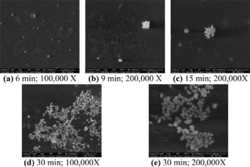
Figure 2: Scanning electron microscopy images obtained from NR/Au samples. Reduction time of gold nanoparticles: from $6$ to $30$ minutes. Magnification: $100,000$ X and $200,000$ X.

The proposed method was applied in the test images with $L=3$ to $L=10$, and precision, recall and accuracy were obtained for each result.

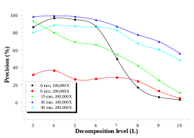
(a) Precision.

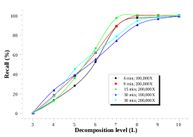
(b) Recall.

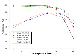
(c) Accuracy.

Figure 3: Precision, recall and accuracy values for Fig. 2 images.

One could see from Fig. 3 that the method accuracy, in general, increases until $L=6$ and starts to decrease when $L=7$. Precision varies widely (between $30\%$ and $100\%$ for $L=3$), but decreases for all images after $L=7$. However, recall has a similar behavior for these images, as $L$ increases.

For a satisfactory segmentation degree, an optimal relationship between $FN$ and $FP$ pixels (i.e. precision and recall) becomes necessary. Optimal $L$ levels were determined based on high accuracy, precision and recall, in order to automatically choose the best result for each image:

• 6 min; 100,000X: from Fig. 3, greater accuracy levels are given for $L$ equals to $5$, $6$ and $7$. $L=6$ (precision = $86,64\%$; recall = $52,42\%$; accuracy = $99,19\%$) was chosen because $L=5$ has a low recall ($28,06\%$) and $L=7$ has a low precision ($49,67\%$), although $L=6$ and $L=7$ have similar accuracy ($98,52\%$ for $L=7$).

• 9 min; 200,000X: although Fig. 3 presents a greater accuracy level for $L=3$, the use of this level is not appropriate, since its recall is almost null. Other levels to be considered are $L$ equals to $6$ and $7$. $L=7$ (precision = $28,49\%$; recall = $89,02\%$; accuracy = $96,58\%$) was chosen because $L=6$ has lower precision ($26,89\%$) and recall ($62,13\%$).

• 15 min; 200,000X: greater accuracy levels are given for $L$ equals to $5$, $6$ and $7$, according to Fig. 3. Even with $L=6$ presenting higher accuracy ($98,18\%$), $L=7$ (precision = $54,82\%$; recall = $97,39\%$; accuracy = $97,80\%$) was chosen by a higher recall value (for $L=6$, $66,38\%$).

• 30 min; 100,000X: also from Fig. 3, greater accuracy values are given for $L$ equals to $7$, $8$ and $9$. $L=8$ (precision = $77,36\%$; recall = $90,39\%$; accuracy = $88,31\%$) has a greater accuracy value, precision higher than $L=9$ ($69,47\%$) and recall higher than $L=7$ ($74,18\%$).

• 30 min; 200,000X: finally, greater accuracy levels are given for $L$ equals to $6$, $7$ and $8$, from Fig. 3. $L=7$ (precision = $81,99\%$, recall = $78,39\%$, accuracy = $86,49\%$) was chosen for having greater accuracy, precision higher than $L=8$ ($67,34\%$) and recall higher than $L=6$ ($62,61\%$).

$L=6$, chosen for Fig. 2 (a), results in six decomposition detail levels. Starlet detail decomposition levels of Fig. 2 (a), from 1 to 6, are presented in Fig. 4.

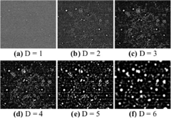
Figure 4: Starlet detail decomposition levels of Fig. 2 (a). $D=1$ and $D=2$ (Fig. 4 (a), (b)) were discarded from algorithm application due to large amount of noise. Higher levels shows nanoparticle locations more clearly; however, background regions tend to aggregate, reducing algorithm accuracy.

Higher detail decomposition levels emphasize the sample surface. The first detail level (Fig. 4 (a)), D1, presents mostly noise; the second level (Fig. 4 (b)), D2, also presents large noise amount. Smoothing factor grows as the decomposition level increases. Higher detail levels ((Fig. 4 (c) to 4 (f)) represents the sample surface with greater precision when the noise decreases, although regions tend to aggregate according to the increasing of detail level.

After starlet application, decomposition levels from $3$ to $6$ (Fig. 4 (c) to 4 (f)) are added and subtracted from the original image (Fig. 2 (a)). The result of Algorithm 1 applied in Fig. 2 (a) is shown in Fig. 5 (a). Similarly, results of Algorithm 1 applied in Fig. 2 (b) to (e) are shown in Fig. 5 (b) to (e).

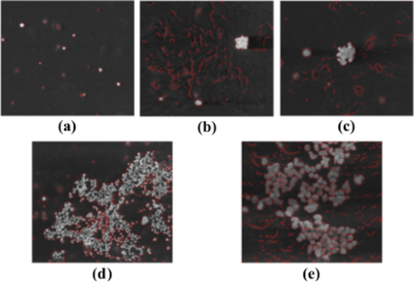
Figure 5: Results of Algorithm 1 applied in Fig. 2. Nanoparticles recognized by the proposed algorithm appear highlighted.

Ground truth (GT) images obtained from Fig. 2 are used to evaluate the performance of the proposed algorithm. These images were acquired manually by a specialist, using GIMP, an open source graphics software.

Results of Algorithm 1 applied in Fig. 2 are represented by binary images, where nanoparticles (the region of interest) are white regions and background by black regions. For comparison effects, green is assigned to true positive (TP) pixels, blue to false negative (FN) pixels and red to false positive (FP) pixels (Fig. 6).

Figure 6: Ground Truth (first column), result of Algorithm 1 application (second column) and comparison (third column) between GT and results. Green: true positive (TP) pixels; blue: false negative (FN) pixels; red: false positive (FP) pixels.

Most gold nanoparticles shown in GT images were located by the proposed method. In some cases, nanoparticles were not completely encountered; this phenomenon is represented by green spots surrounded by blue pixels. False positive results (red pixels) appear mostly in background. This is given by high roughness in the surface of natural rubber samples.

4.1 Inaccurate results

Since the proposed method is aimed at boundary-based segmentation, input images with high natural rubber roughness (as presented in Fig. 6 (b) and (e)) presents higher FP values, which leads to lower algorithm accuracy. SEM images obtained by backscattering detectors do not show surface topology, possibly minimizing this issue. Likewise, a large amount of aggregated nanoparticles leads to a high FN value (Fig. 6 (d)).

5 Conclusion

In this study we present a method for segment scanning electron microscopy images based on starlet wavelets. This algorithm uses starlet decomposition detail levels to determine the edges of objects within an input image. After obtaining the starlet detail levels, the higher detail levels are added and background is removed from this result. Therefore, only the desired details are shown.

An application of the method is shown in images obtained from natural rubber samples with gold nanoparticles. In this application, our method obtained accuracy higher than 85% in images obtained by secondary detectors.

There are some issues concerning the presented method. Structural details of the input image can interfere in the final result, being labeled as desired areas. However, the method presented high accuracy for all dataset images. For better results, we suggest application in SEM images obtained by backscattering detectors, that do not show the surface topology.

Results given by this algorithm will be used in future studies, to computationally estimate the density distribution of gold nanoparticles in natural rubber samples, and also to predict reduction kinetics of gold nanoparticles at different time periods.

References

- [1] F. C. Cabrera, D. L. S. Agostini, R. J. dos Santos, S. R. Teixeira, M. A. Rodriguez-Perez, and A. E. Job, “Characterization of natural rubber/gold nanoparticles sers-active substrate,” Journal of Applied Polymer Science, vol. 130, no. 1, pp. 186–192, 2013.
- [2] P. H. B. Aoki, D. Volpati, F. C. Cabrera, V. L. Trombini, A. R. Jr., and C. J. L. Constantino, “Spray layer-by-layer films based on phospholipid vesicles aiming sensing application via e-tongue system,” Materials Science and Engineering: C, vol. 32, no. 4, pp. 862 – 871, 2012.
- [3] J. S. DuChene, W. Niu, J. M. Abendroth, Q. Sun, W. Zhao, F. Huo, and W. D. Wei, “Halide anions as shape-directing agents for obtaining high-quality anisotropic gold nanostructures,” Chemistry of Materials, vol. 25, no. 8, pp. 1392–1399, 2013.
- [4] A. R. Guerrero and R. F. Aroca, “Surface-enhanced fluorescence with shell-isolated nanoparticles (shinef),” Angewandte Chemie International Edition, vol. 50, no. 3, pp. 665–668, 2011.
- [5] R. C. Gonzalez and R. E. Woods, Digital image processing. Upper Saddle River, N.J: Prentice Hall, 3rd ed ed., 2008.
- [6] D. Sui and K. Wang, “A counting method for density packed cells based on sliding band filter image enhancement,” Journal of Microscopy, vol. 250, pp. 42–49, Apr. 2013.
- [7] A. El Mallahi and F. Dubois, “Separation of overlapped particles in digital holographic microscopy,” Optics Express, vol. 21, p. 6466, Mar. 2013.
- [8] L. Lin, S. Wu, and C. Yang, “A template-based automatic skull-stripping approach for mouse brain MR microscopy,” Microscopy Research and Technique, vol. 76, pp. 7–11, Jan. 2013.
- [9] M. Usaj, D. Torkar, M. Kanduser, and D. Miklavcic, “Cell counting tool parameters optimization approach for electroporation efficiency determination of attached cells in phase contrast images,” Journal of Microscopy, vol. 241, pp. 303–314, Mar. 2011.
- [10] W. Shitong and W. Min, “A new detection algorithm (NDA) based on fuzzy cellular neural networks for white blood cell detection,” IEEE Transactions on Information Technology in Biomedicine, vol. 10, pp. 5–10, Jan. 2006.
- [11] J.-L. Starck and F. Murtagh, Astronomical image and data analysis. Berlin: Springer, 2006.
- [12] F. C. Cabrera, P. H. B. Aoki, R. F. Aroca, C. J. L. Constantino, D. S. dos Santos, and A. E. Job, “Portable smart films for ultrasensitive detection and chemical analysis using SERS and SERRS,” Journal of Raman Spectroscopy, vol. 43, pp. 474–477, Apr. 2012.
- [13] C. G. Barboza-Filho, F. C. Cabrera, R. J. Dos Santos, J. A. De Saja Saez, and A. E. Job, “The influence of natural rubber/Au nanoparticle membranes on the physiology of leishmania brasiliensis,” Experimental Parasitology, vol. 130, pp. 152–158, Feb. 2012.
- [14] M. Holschneider, R. Kronland-Martinet, J. Morlet, and P. Tchamitchian, “A real-time algorithm for signal analysis with the help of the wavelet transform,” in Wavelets (J.-M. Combes, A. Grossmann, and P. Tchamitchian, eds.), pp. 286–297, Berlin, Heidelberg: Springer Berlin Heidelberg, 1990.
- [15] M. Shensa, “The discrete wavelet transform: wedding the a trous and mallat algorithms,” IEEE Transactions on Signal Processing, vol. 40, pp. 2464–2482, Oct. 1992.
- [16] J.-L. Starck, F. Murtagh, and J. Fadili, Sparse image and signal processing: wavelets, curvelets, morphological diversity. Cambridge; New York: Cambridge University Press, 2010.
- [17] A. Genovesio and J.-C. Olivo-Marin, “Tracking fluroescent spots in biological video microscopy,” Proc. SPIE, vol. 4964, pp. 98–105, 2003.
- [18] J.-L. Starck, F. Murtagh, and M. Bertero, “Starlet transform in astronomical data processing,” in Handbook of Mathematical Methods in Imaging (O. Scherzer, ed.), pp. 1489–1531, New York, NY: Springer New York, 2011.
- [19] D. L. Olson and D. Delen, Advanced data mining techniques. Springer, 2008.
- [20] Q. Wang, Y. Yuan, P. Yan, and X. Li, “Saliency detection by multiple-instance learning,” Cybernetics, IEEE Transactions on, vol. 43, no. 2, pp. 660–672, 2013.