metricDTW: local distance metric learning in Dynamic Time Warping
Abstract
We propose to learn multiple local Mahalanobis distance metrics to perform k-nearest neighbor (kNN) classification of temporal sequences. Temporal sequences are first aligned by dynamic time warping (DTW); given the alignment path, similarity between two sequences is measured by the DTW distance, which is computed as the accumulated distance between matched temporal point pairs along the alignment path. Traditionally, Euclidean metric is used for distance computation between matched pairs, which ignores the data regularities and might not be optimal for applications at hand. Here we propose to learn multiple Mahalanobis metrics, such that DTW distance becomes the sum of Mahalanobis distances. We adapt the large margin nearest neighbor (LMNN) framework to our case, and formulate multiple metric learning as a linear programming problem. Extensive sequence classification results show that our proposed multiple metrics learning approach is effective, insensitive to the preceding alignment qualities, and reaches the state-of-the-art performances on UCR time series datasets.
1 Introduction
Dynamic time warping (DTW) is an algorithm to align temporal sequences and measure their similarities. DTW has been widely used in speech recognition [16], human motion synthesis [11], human activity recognition [14] and time series classification [3]. DTW allows temporal sequences to be locally shifted, contracted and stretched, and it calculates a global optimal alignment path between two given sequences under certain restrictions. Therefore, the similarity between two sequences calculated under the optimal alignment is independent of, to some extent, non-linear variations in the time dimension. The similarity is often quantified by the DTW distance, which is the sum of point-wise distances along the alignment path, i.e., , where p is the alignment path between two sequences and , is a pair of matched points on the alignment path and is the distance (affinity) between and . The most widely used point-wise distance is the (squared) Euclidean distance.
Since DTW distance naturally measures the similarity between time series, it is widely used for time series classification. There is increasing acceptance that the nearest neighbor classifier with the DTW distance as the similarity measure (1NN-DTW) is the choice for most time series classification problems and very hard to beat [15, 20, 1, 17]. Although 1NN-DTW is competitive and hard to beat, to the best of our knowledge, the DTW distance is often computed as the sum of point-wise (squared) Euclidean distances along the matching path, i.e., , where is the (squared) Euclidean distance between the matched points and . Nevertheless, the performance of kNN significantly depends on the used similarity measures. Although Euclidean distance is simple and sometimes effective, but it is agnostic of domain knowledge and data regularities. Extensive researches have shown that kNN performances can be greatly improved by learning a proper distance metric (e.g., Mahalanobis distance) from labels examples [21, 2]. This motives us to learn local distance metrics and calculate DTW distance as the sum of point-wise learned distances, i.e., , where , is a positive semidefinite matrix to be learned and is the squared Mahalanobis distance. In the paper, instead of learning one uniform distance metric, we partition the feature space, and learn individual metrics within and between subspaces. When using DTW distance calculated under the learned metrics as the similarity measure, 1NN classifier has the potential to obtain improved performances.
We closely follow Large Margin Nearest Neighbor (LMNN) [21] to formulate local metric learning in DTW. In [21], the Mahalanobis metric is learned with the goal that the k-nearest neighbors always belong to the same class while examples from different classes are separated by a large margin. Mathematically, the authors formulate the metric learning as a semidefinite programming problem. In our case, we use the same max margin framework, with the only difference that: examples in [21] are feature points in some fixed-dimension space, and distances between examples are squared Mahalanobis distances, while in our case, examples are temporal sequences, and distances between examples are DTW distances. We term the local metric learning in DTW as metricDTW. We have to emphasize that although the learned local distances are metric distances, the DTW distance under those metrics is generally not a metric distance since the triangle inequality does not hold.

Before computing the DTW distance, we have to align given sequences to obtain the alignment path, along which the DTW distance is defined. In our work, we do not aim to learn to align sequences, instead, we use existing DTW techniques to align sequences first and treat these alignment paths as known. Therefore, the metric learning in DTW is independent of the preceding alignment process, in principle, any sequence alignment algorithms can be used before metric learning.
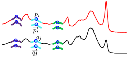
In the paper, different from the tradition, we compute the distance between a matched point pair by the distance between their descriptors. The descriptor of a temporal point is a representation of the subsequence centering on that point, and it represents the structural information around that point (see Fig. 2). In this way, DTW distance is computed as the accumulated descriptor distances along the alignment path. In our case, descriptors are further k-means clustered into groups, then multiple local distance metrics are learned within individual clusters and between any two clusters, such that DTW distances calculated under the learned metrics make kNN neighbors of temporal sequences always come from the same class, while sequences from different classes are separated by a large margin. Our proposed local metrics learning framework is depicted in Fig. 1.
Our multiple metric learning ends up learning multiple Mahalanobis distance matrices, some magnifying the Euclidean distances between subsequences, while other shrinking the original Euclidean distances. This is equivalent to learn the importance of subsequences automatically, e.g., certain shaped subsequences are discriminative for classification, and their subtle differences may be magnified by the corresponding learned metrics, while certain shaped subsequences are less class-membership defining, and their big differences might be suppressed after metric learning. In this perspective, our local metric learning framework is essentially learning the importance of different subsequences in an automatic and principled way.
We extensively test the performance of metricDTW for time series classification on 70 UCR time series datasets [3], and experimental results show that (1) the learned local metrics, compared with the default Euclidean metric, improve the 1NN classification accuracies significantly; (2) given alignment paths of different qualities, the subsequent metric learning consistently boosts classification accuracies significantly, showing that the proposed metric learning approach is invariant to the preceding alignment step; (3) our metric learning algorithm outperforms the state-of-the-art time series classification algorithm (1NN-DTW) significantly on UCR datasets, therefore, we set a new record for future time series classification comparison.
2 Related work
As mentioned, our local metric learning framework is essentially learning the importance of different subsequences in an automatic and principled way. There are several prior works focusing on mining representative and discriminative subsequences (image patches) from temporal sequences (images).
Time series shapelet is introduced in [22], and it is a time series subsequence (patterns) which is discriminative of class-membership. The authors propose to enumerate all possible candidate subsequences, evaluate their qualities using information gain, and build a decision tree classifier out of the top ranked shapelets. Mining shapelets in their case is to search for more important subsequences, while disregarding less important subsequences. In the vision community, there are several related works [19, 5, 4], all of which are devoted to discovering mid-level visual patches from images. Mid-level visual patch is conceptually similar to shapelet in time series, and it a image patch which is both representative and discriminative for scene categories. They [19, 5] pose the discriminative patch search procedure as a discriminative clustering process, in which they selectively choose important patches but discarding other common patches. We are different from above work in that, we never have to greedily select important subsequences, instead, we take all subsequences into account and automatically learn their importance through metric learning.
Our work is most similar to and largely inspired by LMNN [21]. In [21], Weinbergre and Saul extend LMNN to learn multiple local distance metrics, which is exploited in our work as well. However, we are still sufficiently different: first the labeled examples in our case are temporal sequences; second, the DTW distance between two examples is jointly defined by multiple metrics, while in [21], distance between two examples are determined by a single metric. In [7], Garreau et al propose to learn a Mahalanobis distance metric to perform DTW sequence alignment. First they need ground-truth alignments, which is not required in our case, and second they focus on alignment, instead of kNN classification.
3 Local distance metric learning in DTW
As mentioned above, local metric learning needs sequence alignments as inputs. While in most scenarios, ground-truth sequence to sequence alignments are expensive or impossible to label, in experiments, we use DTW to align sequences first, and use the computed alignments for the subsequent metric learning. In this section, we first briefly review the DTW algorithm for sequence alignment, and then introduce our multiple local metric learning algorithm for time series classification.
3.1 Dynamic Time Warping
DTW is an algorithm to align temporal sequences under certain restrictions. Given two sequences and of possible different lengths and , namely and , and let be the pairwise distance matrix, where is the distance between points and . One widely used distance measure is the squared Euclidean distance, i.e., . The goal of temporal alignment between and is to find two sequences of indices and of the same length , which match index in the time series to index in the time series , such that the total cost along the matching path is minimized. The alignment path is constrained to satisfies boundary, monotonicity and step-pattern conditions [18, 13, 7]:
| (1) |
Searching for an optimal alignment path p under the above restrictions is equivalent to solve the following recursive formula:
| (2) |
where is the accumulated distance from the matched point-pair to the matched point-pair along the alignment path, and is the distance between points and . In all the following alignment experiments, we use the squared Euclidean distance to compute . The above formula is a typical dynamic programming recursion, and can be solved efficiently in time by a dp algorithm [6]. The alignment path p is obtained by back-tracking. Various temporal window constraints [18] can be enforced and we could use more complicated step patterns, such as “asymmetric” and “rabinerJuang” [16, 8], but here we consider DTW without warping window constraints and taking moving patterns as defined in (1).
3.2 Local distance metric learning
After obtaining the alignment path p by DTW , we can compute DTW distance between and in two ways: (1) directly return DTW distance as the accumulated distances between matched pairs along p, i.e., ; (2) to measure the distance between a matched pair , we could use the distance between their descriptors, i.e., , where and are descriptors of points and respectively. In this way, DTW distance between and is calculated as the accumulated descriptor distances along p, i.e., . Here, the descriptor at some point is a feature vector representation of the subsequence centering at that point, and the descriptor is supposed to capture the neighborhood shape information around the temporal point (see Fig. 2 for the illustration of descriptors). Using their descriptor distance to measure two point similarity (distance) makes much sense since two point similarity is usually better represented by their neighbor structural similarity, instead of by their single point to point distance.
In following experiments, we always adopt the second way to define the DTW distance, and we use three shape descriptors, namely the raw-subsequence, HOG-1D [23] and the gradient sequence [12].
If the squared Euclidean distance is used, then DTW distance is calculated as , which is essentially a equally weighted sum of distances between descriptors (subsequences), however, as shown in [22], some subsequences are more class-membership predictive, while others are less discriminative. Therefore, it makes more sense, if we calculate the DTW distance as a weighed sum of distances between subsequences, i.e., , where is the weight between two subsequences and and indicates the importance of subsequences and for classification. If we make further generalization, the DTW distance can be calculated as the sum of squared Mahalanobis distances between subsequences, i.e., , where is a positive semidefinite Mahalanobis matrix to be learned from the labeled data. Note that, instead of learning a global metric matrix, we learn multiple local metric matrices simultaneously. The intuition behind is that differently-shaped subsequences have different importance for classification, therefore, their between-distances should be computed under different metrics. In experiments, we first k-means partition the descriptors from all training sequences into clusters, and then learn Mahalanobis distance metrics within individual clusters and between any two different clusters. Let, denote the metrics within the cluster and between two cluster and respectively, and then the distance between any two descriptors and is , where and are clusters and belong to respectively.
In order to learn these local metrics from labeled sequence data, we follow LMNN [21] closely and pose our problem as a max margin problem: the local Mahalanobis metrics are trained such that the k-nearest neighbors of any sequence always belong to the same class while sequences of different classes are separated by a large margin. We use the exact notations in LMNN, and the only place to change is to replace the squared Mahalanobis point-to-point distance in [21] by the DTW distance. The adapted LMNN is as follows:
| (3) |
Note that we enforce the learned matrices between two clusters and to be the same, i.e., , which makes distance mapping between and be a metric. We refer readers to [21] for notation meanings. In our experiments, we further simplify the form of Mahalanobis matrices, and constrain them to be not only diagonal but also with single repeated element on the diagonal, i.e., . Under this simplification, learning a Mahalanobis matrix reduces to learning a scalar, resulting in unknown scalars to learn. Under the reduction, the original semidefinite programming (3) reduces to a linear programming. In experiments, the balancing factor is tuned by cross-validation.
4 Experiments
In this section, we evaluate the performances of the proposed local metric learning method for time series classification on 70 UCR datasets [3], which provide their standard training/test partitions for performance evaluation.
We empirically show below that: (1) whether multiple local metric learning boosts time series classification accuracies of 1NN classifier; (2) how the quality of the preceding alignments affects the subsequent metric learning performances; (3) the influence of hyper-parameter settings on the metric learning performances.
4.1 Experimental settings
Sequence alignment: when running DTW (2) to align sequences, we use the default squared Euclidean distances to compute point-to-point distance. The alignment paths are the inputs of the subsequent metric learning step.
Temporal point descriptors: the descriptor at a temporal point is used to represent its neighborhood structures. When computing the point to point distance in DTW alignment ( in (2)), we compute the distance between their descriptors and use it as the distance between the original temporal points. Obviously, the searched optimal alignment path by DTW (2) depends on the used descriptor for point-to-point distance computations. Descriptors are used in the subsequent metric learning as well to define the DTW distance (see Sec. 3.2).
In experiments, we use three subsequence descriptors, including raw-subsequence, HOG-1D [23] and the derivative sequence [12]. (1) The raw-subsequences taken from temporal points are fixed to be of length 30; (2) HOG-1D is a representation of the raw subsequence, and we use two non-overlapping intervals, use 8 bins and set resulting in a 16D HOG-1D descriptor; (3) the derivative descriptor is simply the first order derivative sequence of the raw subsequence. We follow [12] exactly to compute derivative at each point, and the derivative descriptor is 30D by definition.
Metric learning: k in kNN is set to 3. For each training time series, we compute its 3 nearest neighbors of the same class based on the DTW distances, which is computed under the default Euclidean metric. We set k in k-means to be 5, partition the training descriptors into 5 clusters and local distance metrics are defined within and between these 5 clusters. The linear program (3) is solved by the CVX package [10, 9]. During test, we use the label of its nearest neighbor in the training set as the predicted test label. This is consistent with the convention in the time series community, in which they use 1NN as classifier.
4.2 Effectiveness of local distance metric learning
First, we fix the alignment, and explore the performances of local metric learning. Then, we analyze the influence of the preceding alignment qualities on the performances of subsequent metric learning.
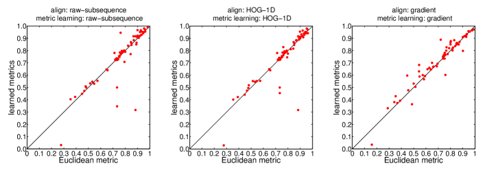
We align time series by DTW under three descriptors, derivative, HOG-1D and raw-subsequence, respectively. Given the computed alignments, we learn local distance metrics under the same descriptor as used in the alignment by solving the LP problem (3), and plot 1NN classification accuracies in Fig. 3. Plots in Fig. 3 are scatter plots showing the comparison between 1NN classifier performances under the Euclidean metric and the learned metrics. Each red dot in the plot indicates one UCR dataset, whose x-mapping and y-mapping are accuracies under the Euclidean metric and the learned metrics respectively. By running the signed rank Wilcoxon test, we obtain p-values 0.038/0.015/0.003 for the descriptor raw-subsequence/HOG-1D/gradient, showing that our proposed metric learning improve the 1NN classifier significantly under the confidence level .
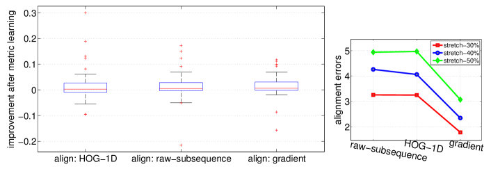
Since the alignment path is the input for the metric learning step, bad alignments may affect the performance. Nevertheless, we empirically show this is not the case. We perform metric learning under different alignments, and evaluate whether significant improvements can be achieved under all cases. In experiments, we align time series under three descriptors, and then learn metrics under the gradient descriptor. We use boxplot to show the performance improvements, compared with using the default Euclidean metric, in Fig. 4(left). The blue box has two tails: the lower and upper edge of each blue box represent 25th and 75th percentiles, with the red line inside the box marking the median improvement and two tails indicating the best and worst improvements. Under three different alignments, the median improvements are all greater than 0 and the majority of improvements are above 0. By running the signed rank Wilcoxon test between the 1NN performances under the Euclidean metric and the learned metrics, we obtain p-values 0.007/0.029/0.003 under alignments by the descriptor raw-subsequence/HOG-1D/gradient. This empirically indicates that the subsequent metric learning is robust to the preceding alignment qualities.
To show different descriptors do have different alignment qualities, we could compare DTW alignment paths under different descriptors against the ground-truth alignments. However, UCR datasets do not have the ground-truth alignments, here we simulate time series alignment pairs by manually scaling and stretching time series, and the ground-truth alignment between the original time series and the stretched one is known by simulation; then we run DTW alignment under different descriptors, evaluate the alignment error against the ground truth, and plot the results in 4(right). It shows different algorithms do perform differently. We refer the readers to the supplementary materials for simulation details.
4.3 Effects of hyper-parameters
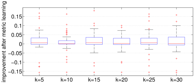
There is one important hyper-parameter in the metric learning: the number of clusters of descriptors. In experiments, we align and learn local metrics both under the gradient descriptor, and during the metric learning, we set different numbers of descriptor clusters, i.e., , learn metrics by solving (3), and plot the 1NN performance improvements in Fig. 5. Under different k’s, the majority of the improvements are above 0, and the signed rank Wilcoxon test returns p-values 0.003/ 0.026/ 0.005/ 0.021/ 0.002/ 0.017 under k=5/10/15/20/25/30, showing significant improvements under varied k’s.
4.4 Comparison with the state of the art algorithm
As shown in [15, 20, 1, 17], 1NN classifier with the DTW distance as the similarity measure (1NN-DTW) is very hard to beat. Here we use 1NN-DTW as the baseline, and compare our algorithms to it. In 1NN-DTW, the alignment is computed by DTW as well, however, no descriptor is used, i.e., the point to point distance is directly computed by the squared Euclidean distance between those two points, instead of by their descriptor distance. The DTW distance between two aligned sequences is computed as the accumulated squared Euclidean point-to-point distances with no descriptor used as well.
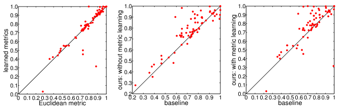
In our case, we use the HOG-1D descriptor to align sequences and learn local metrics. We plot the time series classification performances in Fig. 6: our algorithm with (without) metric learning wins/draws/loses the baseline on 48/3/19 (47/3/20) datasets, and the signed rank Wilcoxon test returns p-values , showing significant accuracy improvement over 1NN-DTW. We document the classification error rates of three algorithms in the supplementary materials.
5 Conclusion and discussion
In this paper, we propose to learn multiple local Mahalanobis distance metrics to perform k-nearest neighbor (kNN) classification of temporal sequences. We showed empirically that the metric learning process always improves the 1NN time series classification accuracies, disregard of the qualities of the preceding DTW alignments. Our algorithm wins the 1NN-DTW algorithm significantly on 70 UCR time series datasets, and sets up a record for further comparison.
DTW time series classification has two consecutive steps: time series alignment and then classification. In this paper, the metric learning happens after the alignment finishes, and information in the metric learning does not back-prop into the preceding alignment step. An naive extension is to do alignment and metric learning in an iterative process. But as we tried, this deteriorated the classification performances. A future research direction is how to do the alignment and learn metrics in an integrated fashion.
References
- [1] A. Bagnall and J. Lines. An experimental evaluation of nearest neighbour time series classification. arXiv preprint arXiv:1406.4757, 2014.
- [2] A. Bellet, A. Habrard, and M. Sebban. A survey on metric learning for feature vectors and structured data. arXiv preprint arXiv:1306.6709, 2013.
- [3] Y. Chen, E. Keogh, B. Hu, N. Begum, A. Bagnall, A. Mueen, and G. Batista. The ucr time series classification archive, July 2015. www.cs.ucr.edu/~eamonn/time_series_data/.
- [4] C. Doersch, A. Gupta, and A. A. Efros. Mid-level visual element discovery as discriminative mode seeking. In Advances in neural information processing systems, pages 494–502, 2013.
- [5] C. Doersch, S. Singh, A. Gupta, J. Sivic, and A. Efros. What makes paris look like paris? ACM Transactions on Graphics, 31(4), 2012.
- [6] D. Ellis. Dynamic time warp (dtw) in matlab, 2003. www.ee.columbia.edu/~dpwe/resources/matlab/dtw/.
- [7] D. Garreau, R. Lajugie, S. Arlot, and F. Bach. Metric learning for temporal sequence alignment. In NIPS, pages 1817–1825, 2014.
- [8] T. Giorgino et al. Computing and visualizing dynamic time warping alignments in r: the dtw package. Journal of statistical Software, 31(7):1–24, 2009.
- [9] M. Grant and S. Boyd. Graph implementations for nonsmooth convex programs. In V. Blondel, S. Boyd, and H. Kimura, editors, Recent Advances in Learning and Control, Lecture Notes in Control and Information Sciences, pages 95–110. Springer-Verlag Limited, 2008. http://stanford.edu/~boyd/graph_dcp.html.
- [10] M. Grant and S. Boyd. CVX: Matlab software for disciplined convex programming, version 2.1. http://cvxr.com/cvx, Mar. 2014.
- [11] E. Hsu, K. Pulli, and J. Popović. Style translation for human motion. ACM Transactions on Graphics, 24(3):1082–1089, 2005.
- [12] E. Keogh and M. Pazzani. Derivative dynamic time warping. In SDM, volume 1, pages 5–7. SIAM, 2001.
- [13] E. Keogh and C. Ratanamahatana. Exact indexing of dynamic time warping. Knowledge and information systems, 7(3):358–386, 2005.
- [14] K. Kulkarni, G. Evangelidis, J. Cech, and R. Horaud. Continuous action recognition based on sequence alignment. IJCV, pages 1–25, 2014.
- [15] F. Petitjean, G. Forestier, G. Webb, A. Nicholson, Y. Chen, and E. Keogh. Dynamic time warping averaging of time series allows faster and more accurate classification. In ICDM, 2014.
- [16] L. Rabiner and B.-H. Juang. Fundamentals of speech recognition. 1993.
- [17] T. Rakthanmanon, B. Campana, A. Mueen, G. Batista, B. Westover, Q. Zhu, J. Zakaria, and E. Keogh. Searching and mining trillions of time series subsequences under dynamic time warping. In SIGKDD, pages 262–270. ACM, 2012.
- [18] H. Sakoe and S. Chiba. Dynamic programming algorithm optimization for spoken word recognition. IEEE Transactions on Acoustics, Speech and Signal Processing, 26(1):43–49, 1978.
- [19] S. Singh, A. Gupta, and A. Efros. Unsupervised discovery of mid-level discriminative patches. Computer Vision–ECCV 2012, pages 73–86, 2012.
- [20] X. Wang, A. Mueen, H. Ding, G. Trajcevski, P. Scheuermann, and E. Keogh. Experimental comparison of representation methods and distance measures for time series data. DMKD, 26(2):275–309, 2013.
- [21] K. Q. Weinberger and L. K. Saul. Distance metric learning for large margin nearest neighbor classification. The Journal of Machine Learning Research, 10:207–244, 2009.
- [22] L. Ye and E. Keogh. Time series shapelets: a new primitive for data mining. In SIGKDD, pages 947–956. ACM, 2009.
- [23] J. Zhao and L. Itti. Decomposing time series with application to temporal segmentation.