From Generalized Langevin Equations to Brownian Dynamics and Embedded Brownian Dynamics

Abstract

We present the reduction of generalized Langevin equations to a coordinate-only stochastic model, which in its exact form, involves a forcing term with memory and a general Gaussian noise. It will be shown that a similar fluctuation-dissipation theorem still holds at this level. We study the approximation by the typical Brownian dynamics as a first approximation. Our numerical test indicates how the intrinsic frequency of the kernel function influences the accuracy of this approximation. In the case when such an approximate is inadequate, further approximations can be derived by embedding the nonlocal model into an extended dynamics without memory. By imposing noises in the auxiliary variables, we show how the second fluctuation-dissipation theorem is still exactly satisfied.

I Introduction

The Langevin dynamics (LD) model plays a crucial role in the stochastic modeling of bio-molecules Schlick2002 . In general, the LD model can be expressed as follows,

$$m\ddot{x}=f(x)-\gamma\dot{x}+\xi(t).$$ (1)

Here $m$ denotes the mass, $f(x)$ is the inter-molecular force, and $\gamma$ is the friction coefficient. In addition, $\xi(t)$ is an external white noise, which satisfies the fluctuation-dissipation theorem (FDT) Kubo66 ,

$$\Big{\langle}\xi(t)\xi(t^{\prime})^{T}\Big{\rangle}=2k_{B}T\gamma\delta(t-t^{\prime}).$$ (2)

This condition ensures that the dynamical system settles to the correct equilibrium Kubo66 .

In the Langevin dynamics model (1), the damping coefficient and the random noise are modeling the influence of the solvent particles. One interesting regime is where $\gamma\gg 1.$ The asymptotic analysis has been the subject of theoretical interest. The analysis can be done either through the Fokker-Planck equation titulaer1980corrections ; titulaer1978systematic using the Chapman-Enskog expansion, or directly based on the stochastic differential equation san1980colored . In Ref. san1980colored , the LD model was written in the first order form, and by solving the second equation, the velocity variables can be eliminated. These analysis confirms that, when the damping is large, the inertial term can be neglected, leading to,

$$\gamma\dot{x}=f(x)+\xi(t).$$ (3)

This model has been referred by some authors as the Brownian dynamics (BD) model huber2010browndye ; ricci2003algorithms ; van1982algorithms . Notice that in this reduced model, $\xi(t)$ still obeys the FDT (2).

The derivation of the Brownian dynamics is of obvious theoretical interest. In practice, the BD (3) neglects the transient time scale, and as a result, the dynamics occurs on a much larger time scale. Therefore, from a computational viewpoint, the time step can be much larger than that of the original Langevin dynamics (1). This model is of considerable advantage in bio-molecular simulations, in which the time scale of interest is often out of reach when the full model (1) is used.

There have been important theoretical works toward the asymptotic analysis in the limit of large damping coefficients. The question of high friction limit also arises in the study of plasma gases, especially those involving nonlocal Coulomb interactions, with kinetic descriptions el2010diffusion ; goudon2005hydrodynamic ; goudon2005multidimensional ; poupaud2000parabolic ; nieto2001high . In our recent work wu2015diffusion , we studied a Vlasov-Poisson-Fokker-Planck (VPFP) system in a bounded domain with reflection boundary conditions for charge distributions, showed the convergence to the macroscopic Poisson-Nerest-Planck (PNP) system. The purpose there was trying to justify the PNP system as a macroscopic model for the transport of multi-species ions in dilute solutions.

The BD model (3) can be viewed as a first order approximation to the full Langevin dynamics model (3). Meanwhile, there have been numerous attempts to derive high order approximations to improve the modeling accuracy without having to resolve the small time scales. A remarkable success is the inertial Brownian dynamics model (IBD), developed by Beard and Schlick beard2000inertial ; beard2000inertialB . Using further asymptotic expansions, the IBD incorporates correction terms into the BD model and takes into account the transient part of the dynamics.

Motivated by these effort, we study the BD approximation of the generalized Langevin equation (GLE). In contrast to the Langevin dynamics (1), the GLE includes a history-dependent friction term and a correlated Gaussian noise. The memory term often comes from a coarse-graining step, e.g., AdDo74 ; tully1980dynamics ; guardia1985generalized ; ciccotti1981derivation ; LiXian2014 ; ChSt05 ; curtarolo_dynamics_2002 ; espanol2004statistical ; EvMo08 ; IzVo06 ; Li2009c ; Li14 ; LiE07 ; li2015incorporation ; MaLiLiu16 ; oliva2000generalized ; stepanova_dynamics_2007 ; Zwanzig73 ; lei2016generalized , which has also been an recent emerging area of interest in molecular modeling. Among the many approximation schemes berkowitz1983generalized ; berkowitz1981memory ; LiXian2014 ; Darve_PNAS_2009 ; hijon2010mori ; kauzlaric2011bottom ; MaLiLiu16 ; oliva2000generalized for the GLE model, the BD model (3) is clearly the simplest. To understand how the BD approximation can naturally come about, we first present a derivation which eliminates momentum variables from the GLE, so that the resulting model only involves the coordinates of the molecular variables. It will be proved that the reduced model still exhibits history-dependence, and the second fluctuation-dissipation theorem, an important property of the GLE, is inherited by the reduced model, just like the BD approximation of the full Langevin dynamics.

At this level, the BD approximation arises as the first approximation, in which the memory kernel is approximated by a Dirac delta function. To understand the accuracy and possibly, the limitation of this approximation, we consider the GLE derived by Adelman and Doll AdDo74 ; AdDo76 , and conducted several numerical tests. Our results indicate that the accuracy hinges on the frequency associated with the memory kernel: When the frequency is large, compared to that of the mean force, the approximation by BD is quite promising. Otherwise, the accuracy is quite limited and high order approximations are needed. To improve the modeling accuracy, we derive two other approximations where the memory kernel is approximated by rational functions in the Laplace domain. The main motivation has been two-fold: On one hand, in the time domain, the memory can be eliminated by introducing auxiliary variables. As a result, there is no need to keep the history of the solution and evaluate the integral associated with the memory term at every step. This significantly suppresses the computational cost. Meanwhile, it will be shown that with proper choices of the stochastic forces, applied to the auxiliary variables, the noise in the GLE is approximated by a colored noise, in such a way that the second FDT is exactly satisfied.

II Mathematical Derivation

We start with the generalized Langevin equations (GLE),

$$\left\{\begin{aligned} \dot{x}=&v,\\ \dot{v}=&f(x)-\gamma v-\int_{0}^{t}\theta(t-\tau)v(\tau)d\tau+\xi(t).\end{aligned}\right.$$ (4)

The mass has been set to unity. The random noise is assumed to be a mean-zero Gaussian process, with time correlation given by,

$$\Big{\langle}\xi(t)\xi(t^{\prime})^{T}\Big{\rangle}=2k_{B}T\gamma\delta(t-t^{\prime})+k_{B}T\theta(t-t^{\prime}).$$ (5)

This is a general form of the fluctuation-dissipation theorem (FDT) Kubo66 . Equation of this form has been derived in our previous work MaLiLiu16 , where the full model is the Langevin dynamics.

We first assume that $\theta$ and $\gamma$ are symmetric, matrix-valued functions. Our goal is simply solving the second equation, and then making a direct substitution into the first equation to eliminate $v(t)$ entirely. For this purpose, we define a matrix-valued function $\chi,$ which satisfies the following equation,

$$\dot{\chi}=-\gamma\chi-\int_{0}^{t}\theta(t-\tau)\chi(\tau)d\tau,\quad\chi(0)=I.$$ (6)

Through Laplace transform, one can show that the function $\chi$ is symmetric. Now $\chi$ can be viewed as the fundamental function associated with the GLE model (4). In particular, we have,

$$v(t)=\chi(t)v(0)+\int_{0}^{t}\chi(t-\tau)\xi(\tau)d\tau+\int_{0}^{t}\chi(t-\tau)f\big{(}x(\tau)\big{)}d\tau.$$ (7)

Let us first look at the first two terms, denoted by $w(t)$

$$w(t)=\chi(t)v(0)+\int_{0}^{t}\chi(t-\tau)\xi(\tau)d\tau.$$ (8)

We assume that $v(0)$ is sampled from its equilibrium. Namely it is Gaussian with mean zero and covariance $k_{B}TI.$ Then the following result can be established using the FDT (5): $w(t)$ is a stationary Gaussian process with mean zero and time correlation given by,

$$\Big{\langle}w(t)w(t^{\prime})^{T}\Big{\rangle}=k_{B}T\chi(t-t^{\prime}),\;\forall t\geq t^{\prime}.$$ (9)

The proof is postponed to the appendix due to some non-trivial calculations.

With this result, we arrive at a Brownian dynamics with memory,

$$\dot{x}=\int_{0}^{t}\chi(t-\tau)f\big{(}x(\tau)\big{)}d\tau+w(t).$$ (10)

Together with (8), this forms a closed set of equations, since a stationary Gaussian process is uniquely determined by its time correlation Doob44 .

To arrive at a conventional BD model (3), we may approximate the kernel function by,

$$\chi(t)\approx 2\chi_{\infty}\delta(t),\quad\chi_{\infty}=\int_{0}^{+\infty}\chi(t)dt,$$ (11)

and we obtain,

$$\dot{x}(t)=\chi_{\infty}f(x(t))+w(t).$$ (12)

In order to preserve the FDT (9), the noise now has to be approximated by a white noise, with covariance given by,

$$\Big{\langle}w(t)w(t^{\prime})^{T}\Big{\rangle}=2k_{B}T\chi_{\infty}\delta(t-t^{\prime}).$$ (13)

This is exactly the standard Brownian dynamics model (3). The coefficients are determined from the formula (11), which is clearly of linear-response type. Namely, we have,

$$\chi_{\infty}=\frac{1}{2k_{B}T}\int_{0}^{+\infty}\Big{\langle}w(t)w(0)^{T}\Big{\rangle}dt.$$

In the next section, we will examine the validity of this approximation.

III A Case Study

To test the approximation (12) presented in the previous section, we consider the GLE model derived by Adelman and Doll AdDo74 ; AdDo76 , in which a gas molecule near a solid surface was considered. We write the position of the gas molecule as $y(t)$ and the position of the solid atom at the surface as $x(t).$ Starting from a one-dimensional chain of solid atoms, Adelman and Doll AdDo74 used Laplace transform, together with a spatial reduction procedure, and derived a GLE for $x(t)$ and $y(t)$ with the remaining solid atoms eliminated. The GLE can be written as,

$$\left\{\begin{aligned} M\ddot{y}=&-\phi^{\prime}(x-y),\\ \ddot{x}=&\phi^{\prime}(x-y)-\gamma\dot{x}-\int_{0}^{t}\theta(t-\tau)\dot{x}(\tau)d\tau+R(t).\end{aligned}\right.$$ (14)

Here $M$ is the mass of the gas molecule, and as in the original work AdDo74 , we set the mass of the solid atom to unity. We write the memory term as a friction term with $\dot{x}$ involved. This way, the FDT is directly expressed as,

$$\big{\langle}R(t)R({\color[rgb]{0,0,0}t^{\prime}})\big{\rangle}=k_{B}T\theta(t-t^{\prime})+2k_{B}T\gamma\delta(t-t^{\prime}).$$ (15)

We also add the damping term with coefficient $\gamma$ to offer a slightly more general setup.

When the one-dimensional chain of solid atoms is infinite, an explicit formula for the kernel function can be found via Laplace transform, and it is given by,

$$\theta(t)=\frac{\omega_{0}}{t}J_{1}(2\omega_{0}t),$$ (16)

where $J_{1}$ is the Bessel function of the first kind, and $\omega_{0}=\sqrt{K}$ with $K$ being the spring constant of the atom chain. This model has been considered by LiE07 ; LiE06 ; liu2006nano to study boundary conditions for molecular dynamics models. Although this explicit formula might be already known to others, we have not found earlier references to it. This kernel function has very slow decay rate, which makes it a highly non-trivial test problem. In light of the natural time scaling in (16), we will consider $\omega_{0}$ as the natural frequency associated with the kernel function, and it represents the corresponding time scale. To make this model more explicit, we choose the Morse potential for the interaction of the gas/solid molecules at the interface,

$$\varphi(u)=(e^{-au}-1)^{2}.$$ (17)

$a$ is chosen as 1, so the vibration frequency associated with the force $f(x)$ is $\omega=\sqrt{2}.$ To further simplify the model, we fix $y=0,$ so that only the second equation in (14) needs to be solved.

The Laplace transform of the kernel function is given by,

$$\Theta(s)=\frac{\sqrt{s^{2}+4\omega^{2}_{0}}}{2}-\frac{s}{2}.$$ (18)

This will be needed in the approximation schemes presented here and the ones in the next section. In particular, we obtain,

$$\chi_{\infty}=\frac{1}{\gamma+\omega_{0}}.$$ (19)

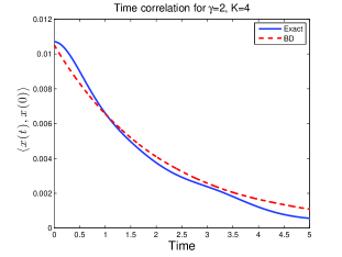
Figure 1: Comparison of the time correlation functions for the full model and the BD model (12). $\gamma=2,K=4$.

To examine the accuracy, we first run the full dynamics with 8192 solid atoms and generate the trajectory of the solid atom at the gas/solid interface. We use the stochastic velocity-Verlet method van1982algorithms to simulate the Langevin dynamics model. The time correlation function $\Big{\langle}x(t),x(0)\Big{\rangle}$ as a dynamic property is regarded as the exact result. As comparison, we solve the BD model (3) with the effective damping coefficients given by (19) using the Euler-Maruyama method. We first choose $\gamma=2,$ and $K=4$, which implies $\omega_{0}=2$. Figure 1 displayed the two time correlation functions. One can see that the results agree quite well, indicating that in this regime, the approximation by the BD model (3) is good.

In the next test, we set $K=0.2$, which gives a much lower frequency. The results are shown in Figure 2, from which we observe discrepancies between the results. In this case, the approximation leads to much bigger error.

Figure 2: Comparison of the time correlation functions for the full model and the BD model (12). $\gamma=2,K=0.2$.

Next, we repeat these experiments with $\gamma=0.$ In this case, the damping mechanism, e.g., $\chi_{\infty}$, can be directly attributed to the friction kernel $\theta.$ When $K=4,$ it turns out that BD is still a reasonable approximation. However, when $K=0.2,$ the time correlation exhibits pronounced oscillations, which is not captured by the BD model, as shown in Figure 3.

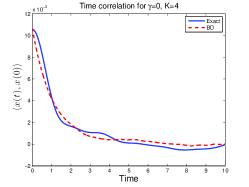
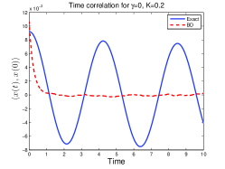
Figure 3: Comparison of the time correlation functions for $\gamma=0,$ $K=4$ (left) and $K=0.2$ (right).

IV Embedded Brownian Dynamics

It has been observed from the previous section that in the regime where $\omega_{0}\ll\omega$, the Brownian dynamics might not be a good approximation to the original dynamics. In this case, we propose to embed the reduced model (10) in an extended system, where the memory is removed and the general Gaussian noise is generated from the additional equations.

More specifically, the approximation is done in terms of the Laplace transform of the kernel function, given by,

$$X(s)=\Big{[}sI+\gamma+\Theta(s)\Big{]}^{-1}.$$ (20)

We seek a rational approximation, in the form of $R(s)=Q(s)^{-1}P(s),$ where $P$ and $Q$ are matrix polynomials, given by,

$$P(s)= A_{0}s^{n-1}+A_{1}s^{n-1}+\cdots+A_{n},$$ (21)

$$Q(s)= s^{n}I-B_{0}s^{n-1}-B_{1}s^{n-1}+\cdots+B_{n}.$$

Here $n$ indicates the level of approximation.

For the zeroth level approximation, we have a constant function and we choose to match the limit as $s\to 0.$ We obtain,

$$\lim_{s\to 0}X=\Big{[}\gamma+M_{\infty}\Big{]}^{-1},$$ (22)

with $M_{\infty}=\lim_{s\to 0}\Theta$. This limit is defined as $\chi_{\infty}$. Namely, we choose $R(s)=\chi_{\infty}.$ With this constant approximation in the Laplace domain, we have a corresponding approximation in the time domain, which gives exactly the BD model (12).

We now turn to higher-order rational approximations. For $n=1$, we write $R_{1,1}(\lambda)=[1-\lambda B]^{-1}A\lambda$, where $\lambda=1/s.$ Similarly we rewrite $X$ as a function of $\lambda$,

$$X(\lambda)=\Big{[}I+\lambda\gamma+\lambda\Theta(\lambda)\Big{]}^{-1}\lambda,$$ (23)

and approximate this Laplace transform by $R_{1,1}$.

From the definition of the Laplace transform, it is clear that $X,R\to 0$, as $\lambda\to 0.$ To determine the matrices $A$ and $B$, we impose the following matching conditions:

$$\begin{split}&\lim_{\lambda\to+\infty}X(\lambda)=\lim_{\lambda\to+\infty}R_{1,1}(\lambda),\\ &\lim_{\lambda\to 0_{+}}\frac{d}{d\lambda}X(\lambda)=\lim_{\lambda\to 0_{+}}\frac{d}{d\lambda}R_{1,1}(\lambda).\end{split}$$ (24)

Direct calculations yield,

$$A=I,\quad B=-(\gamma+M_{\infty}).$$ (25)

This is equivalent to approximating $\chi(t)$ as matrix-exponential function,

$$\chi(t)\approx\chi_{I}(t)\overset{\text{def}}{=}e^{Bt}.$$ (26)

The rational approximation in the Laplace domain makes it possible to eliminate the memory by introducing auxiliary variables. We set $z=\int_{0}^{t}\chi_{I}(t-\tau)f(x(\tau))d\tau$ in (3) as the memory function, then we write an ODE for $z$:

$$\dot{z}=Bz+f,\quad z(0)=0.$$ (27)

We now show that by adding a white noise in this equation, i.e., we have,

$$\left\{\begin{aligned} &\dot{x}=z,\\ &\dot{z}=Bz+f(x)+\xi(t),\\ \end{aligned}\right.$$ (28)

the Gaussian noise $w(t)$ in the exact reduced model (10) can be approximated so that the correlation function is exactly consistent with the approximation by $\chi_{I}(t).$

To prove this statement, let $\Sigma$ be the covariance the noise, i.e.,

$$\langle\xi(t)\xi(t^{\prime})^{T}\rangle=\Sigma\delta(t-t^{\prime}).$$

Then by solving $z$ analytically, we have the expression:

$$z(t)=e^{Bt}z(0)+\int_{0}^{t}e^{B(t-\tau)}\xi(\tau)d\tau+\int_{0}^{t}e^{B(t-\tau)}f(x(\tau))d\tau.$$

Notice the third term of $z(t)$ is exactly the approximation of the memory term with the memory kernel given by $\chi_{I}(t)$. Let the covariance of $z(0)$ be $Q=k_{B}TI$. Then the first two terms form a stationary Gaussian process, provided that the covariance $\Sigma$ satisfies the Lyapunov equation risken1984fokker :

$$-\Sigma=BQ+QB^{T}.$$ (29)

Furthermore, the time correlation of the stationary noise is given by $e^{B(t-t^{\prime})}Q$, which is exactly $\chi_{I}(t)$, therefore the FDT as in (9) is satisfied.

It is clear that this procedure can be extended to higher order. For example, to construct the approximation for $n=2$, we set,

$$R_{2,2}=[I-\lambda B_{0}-\lambda^{2}B_{1}]^{-1}[\lambda A_{0}+\lambda^{2}A_{1}].$$ (30)

To determine the coefficient matrices, we impose the following four conditions,

$$\lim_{\lambda\to+\infty}X(\lambda)=\lim_{\lambda\to+\infty}R_{1,1}(\lambda),$$ (31)

$$\lim_{\lambda\to 0_{+}}\frac{d^{\ell}}{d\lambda^{\ell}}X(\lambda)=\lim_{\lambda\to 0_{+}}\frac{d^{\ell}}{d\lambda^{\ell}}R_{1,1}(\lambda),\quad\ell=1,2,3.$$

The explicit form of the solutions for the coefficients $A_{0},A_{1},B_{0},$ and $B_{1}$ can be found in the appendix.

We let the corresponding approximate kernel function be $\chi_{\textrm{II}}(t),$ which is the inverse Laplace transform of $R_{2,2}.$ Similar to the previous approximation, the memory term can be embedded into an extended system with auxiliary variables $z$ and $z_{1},$ together with the white noises $\xi_{1}$ and $\xi.$ The extended system of equations read,

$$\left\{\begin{aligned} &\dot{x}=z,\\ &\dot{z}_{1}=B_{1}z+A_{1}f+\xi_{1},\\ &\dot{z}=z_{1}+B_{0}z+A_{0}f+\xi.\end{aligned}\right.$$ (32)

Through Laplace transform and direct substitutions, one can easily check that the memory function $\chi$ is approximated by $\chi_{\textrm{II}}(t)$, with the inverse Laplace transform given by (30). The random noise $w(t)$ is also approximated by a Gaussian noise that satisfies the FDT (9) with proper choices of the initial conditions for $z(t)$ and $z_{1}(t)$ and the covariance of the noises $\xi_{1}$ and $\xi$. The details can be found in Appendix C.

Now we turn to the test problem and compare the results from these models. In Figure 4, we present a comparison between different orders of approximations to the exact kernel function for $\gamma=2$. The left panel is for $K=4$ while the right panel is for $K=0.2$. We did not plot the zeroth order approximation (the BD model (12)) since it is a delta function. We want to comment on how we produced the exact result. While the explicit expression of $\theta(t)$ is stated in (16), the exact form of $\chi(t)$ is however nontrivial, which involves integral of highly oscillatory Bessel functions. We therefore adopt a numerical Euler method to invert Laplace transform abate2006unified and name it as Exact Euler. This exact result is tested against high-order numerical quadrature to ensure its accuracy.

One can observe from the graph in Figure 4 that for smaller frequency in the memory kernel $\theta(t)$, the kernel function $\chi(t)$ is more flat, as shown in the graph on the right, and we have improved accuracy from the rational approximations $R_{1,1}$. At the same time, it is obvious that with higher order of approximation $R_{2,2}$, we achieve better results. Next we repeat test for $\gamma=0$. In this case, $\chi$ can be explicitly expressed as

$$\chi(t)=\frac{J_{1}(2\omega_{0}t)}{t\omega_{0}}.$$

Results are shown in Figure 5, and it is clear that for this case, much larger error is introduced in the first order approximation. Though the second order approximation offers better agreement, there is still obvious discrepancy. Therefore we carried out a third order approximation in a similar algorithm, and clearly observe the tendency of convergence to the exact kernel function. Similar to the situation for $\gamma=4$, for smaller frequency in $\theta(t)$, the kernel function is more flat.

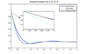
Figure 4: Comparison of the kernel functions for the exact result, the first order rational approximation (26), and the second order approximation (51). $\gamma=2$, $K=4$ (left), $K=0.2$ (right).

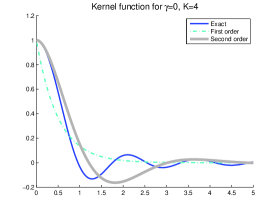
Figure 5: Comparison of the kernel functions. $\gamma=0$, $K=4$ (left), $K=0.2$ (right).

Next, we compare the time correlation of all the cases mentioned. For $\gamma=2$, $K=4,$ the results are collected in Figure 6. In this case, all the approximations, including the BD model (12), the first order rational approximation (28), and the second order approximation (LABEL:eq:_n=2), yield reasonable results. The second order method offers the best approximation over short time scale, this is consistent with increased accuracy near $t=0$ in the approximations.

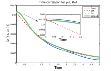
Figure 6: Comparison of the time correlation functions for the full model, the BD model (3), the first order rational approximation (28), and the second order approximation (LABEL:eq:_n=2). $\gamma=2,K=4$.

Meanwhile, for a lower frequency from the kernel, where $K=0.2,$ the results are shown in Figure 7. We observe that as the order of approximation increases, the accuracy is significantly improved. The insets in both Figure 6 and 7 showed that, for higher order of approximations, derivatives near $t=0$ are better predicted.

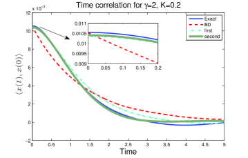
Figure 7: Comparison of the time correlation functions. $\gamma=2,K=0.2$.

We also repeated these experiments with $\gamma=0.$ When $K=4,$ all the approximations give reasonable predictions. One can clearly see the improvement near zero as approximation order gets higher, due to more conditions are matched at zero. However, when $K=0.2,$ the large oscillations in the time correlation are not captured by the BD model as shown in Figure 8. The first order method does predict oscillations, but with the wrong magnitude. The second order method provides the better approximation, and third order is definitely the best among all.

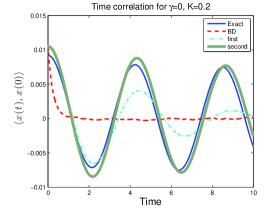
Figure 8: Comparison of the time correlation functions among the approximate models for $\gamma=0,$ $K=4$ (left) and $K=0.2$ (right).

V Summary and Discussions

In this paper we considered the reduction of the generalized Langevin equations to a Brownian dynamics with memory (nonlocal) and correlated noise, then to the standard Brownian dynamics as well as higher order approximations. Due to the considerable advantage of the Brownian dynamics model over Langevin or generalized Langevin dynamics in allowing much larger time steps and longer time scale, it is important to understand the accuracy of such approximations. Our findings gave insight into when to use the simplest BD model and how to reduce the error by using high order approximations.

In our numerical experiments, we chose the memory kernel of the GLE model derived by Adelman and Doll AdDo74 . The corresponding memory kernel exhibits very slow decay, which makes it a good candidate to understand the modeling error. Our interest was in finding the appropriate regime where the Brownian dynamics is a good approximation for the GLE model. In particular, numerous experiments with various frequencies ($\omega_{0}$) of the memory kernel were conducted, while fixing the vibration frequency $\omega$ associated with the potential of mean forces. Our observations have been that the Brownian dynamics is a reasonably good approximation in cases when $\omega_{0}$ is relatively large.

Meanwhile, the Brownian dynamics model will generate large error in the case of low frequency in the memory kernel. We derived high order approximations, by embedding the nonlocal Brownian dynamics model into an extended, local stochastic dynamics. We have shown that by correctly choosing the covariance for the additive noises and the auxiliary variables, the second fluctuation-dissipation theorem are exactly satisfied. Our numerical results showed improved accuracy as the order of the approximation is increased.

At the same time, the current approach for constructing high order approximations can be extended/improved. For example, in constructing our models, we only used interpolations of the Laplace transform at $\lambda=0$ and $\lambda=+\infty$. It is possible to introduce more interpolation points to better resolve the intermediate rescales.

VI Acknowledgment

This research was supported by NSF under grant DMS-1412005, DMS-1216938 and DMS-1619661.

VII Appendix

VII.1 Stationary Gaussian process $w(t)$

In this section, we will prove the statement made in section II. Namely, we will show that $w(t)$ is indeed a stationary Gaussian process satisfying the stated property. More specifically, we want to show that $\Big{\langle}w(t)w(t^{\prime})^{T}\Big{\rangle}$ is a function of $(t-t^{\prime})$, which is equivalent to showing

$$\frac{d}{ds}\Big{\langle}w(t+s)w(t^{\prime}+s)^{T}\Big{\rangle}=0,$$

for any $s.$ Consequently, by taking $s=-t^{\prime}$,

$$\Big{\langle}w(t)w(t^{\prime})^{T}\Big{\rangle}=\Big{\langle}w(t-t^{\prime})w(0)^{T}\Big{\rangle},$$

which shows the stationarity of the random process.

Recall that

$$w(t)=\chi(t)v(0)+\int_{0}^{t}\chi(t-\tau)\xi(\tau)d\tau,$$

and

$$\Big{\langle}\xi(t)\xi(t^{\prime})^{T}\Big{\rangle}=2k_{B}T\gamma\delta(t-t^{\prime})+k_{B}T\theta(t-t^{\prime}),$$

together with the property that $\chi(t)$ is symmetric. For $t\geq t^{\prime}$, the correlation can be written as

$$\Big{\langle}w(t+s)w(t^{\prime}+s)^{T}\Big{\rangle}$$

$$= \chi(t+s)\Big{\langle}v(0)v(0)^{T}\Big{\rangle}\chi(t^{\prime}+s)+\int_{0}^{t+s}\int_{0}^{t^{\prime}+s}\chi(t+s-\tau)\Big{\langle}\xi(\tau)\xi(\tau^{\prime})^{T}\Big{\rangle}\chi(t^{\prime}+s-\tau^{\prime})d\tau^{\prime}d\tau$$

$$= k_{B}T\chi(t+s)\chi(t^{\prime}+s)$$

$$+2k_{B}T\int_{0}^{t^{\prime}+s}\chi(t+s-\tau^{\prime})\Gamma\chi(t^{\prime}+s-\tau^{\prime})d\tau^{\prime}$$

$$+k_{B}T\int_{0}^{t+s}\int_{0}^{t^{\prime}+s}\chi(t+s-\tau)\theta(\tau-\tau^{\prime})\chi(t^{\prime}+s-\tau^{\prime})d\tau^{\prime}d\tau.$$

We denote these terms as term I, II, III respectively.

Taking derivatives with respect to $s$ to each term, we find: For Term I, we have:

$$\frac{d}{ds}\chi(t+s)\chi(t^{\prime}+s)=\dot{\chi}(t+s)\chi(t^{\prime}+s)+\chi(t+s)\dot{\chi}(t^{\prime}+s)$$

$$= \left(-\chi(t+s)\Gamma-\int_{0}^{t+s}\chi(\tau)\theta(t+s-\tau)d\tau\right)\chi(t^{\prime}+s)+\chi(t+s)\left(-\Gamma\chi(t^{\prime}+s)-\int_{0}^{t^{\prime}+s}\theta(t^{\prime}+s-\tau)\chi(\tau)d\tau\right)$$

$$= -2\chi(t+s)\Gamma\chi(t^{\prime}+s)-\int_{0}^{t+s}\chi(\tau)\theta(t+s-\tau)\chi(t^{\prime}+s)d\tau-\int_{0}^{t^{\prime}+s}\chi(t+s)\theta(t^{\prime}+s-\tau)\chi(\tau)d\tau,$$

for Term II, we have:

$$2\frac{d}{ds}\int_{0}^{t^{\prime}+s}\chi(t+s-\tau^{\prime})\Gamma\chi(t^{\prime}+s-\tau^{\prime})d\tau^{\prime}=2\chi(t+s-(t^{\prime}+s))\Gamma\chi(t^{\prime}+s-(t^{\prime}+s))$$

$$+2\int_{0}^{t^{\prime}+s}\dot{\chi}(t+s-\tau^{\prime})\Gamma\chi(t^{\prime}+s-\tau^{\prime})d\tau+2\int_{0}^{t^{\prime}+s}{\chi}(t+s-\tau^{\prime})\Gamma\dot{\chi}(t^{\prime}+s-\tau^{\prime})d\tau^{\prime}$$

$$= 2\chi(t-t^{\prime})\Gamma\chi(0)-2\int_{0}^{t^{\prime}+s}\frac{d}{d\tau^{\prime}}\left(\chi(t+s-\tau^{\prime})\Gamma\chi(t^{\prime}+s-\tau^{\prime})\right)d\tau^{\prime}$$

$$= 2\chi(t-t^{\prime})\Gamma\chi(0)-2\chi(t+s-\tau^{\prime})\Gamma\chi(t^{\prime}+s-\tau^{\prime})\Big{|}_{\tau^{\prime}=0}^{t^{\prime}+s}$$

$$= 2\chi(t+s)\Gamma\chi(t^{\prime}+s),$$

and for Term III:

$$\frac{d}{ds}\int_{0}^{t+s}\int_{0}^{t^{\prime}+s}\chi(t+s-\tau)\theta(\tau-\tau^{\prime})\chi(t^{\prime}+s-\tau^{\prime})d\tau^{\prime}d\tau$$

$$\xlongequal{\text{$u=t^{\prime}+s-\tau^{\prime}$}} \frac{d}{ds}\int_{0}^{t+s}\int_{0}^{t^{\prime}+s}\chi(t+s-\tau)\theta(\tau-(t^{\prime}+s-u))\chi(u)dud\tau$$

$$\xlongequal{\text{$v=t+s-\tau$}} \frac{d}{ds}\int_{0}^{t+s}\int_{0}^{t^{\prime}+s}\chi(v)\theta(t-t^{\prime}-v+u)\chi(u)dudv$$

$$= \int_{0}^{t^{\prime}+s}\chi(t+s)\theta(t-t^{\prime}-(t+s)+u)\chi(u)du+\int_{0}^{t+s}\chi(v)\theta(t-t^{\prime}-v+(t^{\prime}+s))\chi(t^{\prime}+s)dv$$

$$= \int_{0}^{t^{\prime}+s}\chi(t+s)\theta(t^{\prime}+s-\tau)\chi(\tau)d\tau+\int_{0}^{t+s}\chi(\tau)\theta(t+s-\tau))\chi(t^{\prime}+s)d\tau.$$

Notice that the last equation used the property that $\theta$ is an even function. It is clear that the summation of all the three terms gives zero, which shows the stationarity.

Now we have for $t\geq t^{\prime}$,

$$\Big{\langle}w(t)w(t^{\prime})^{T}\Big{\rangle}=\Big{\langle}w(t-t^{\prime})w(0)^{T}\Big{\rangle}$$

$$= \Big{\langle}\left(\chi(t-t^{\prime})v(0)+\int_{0}^{t-t^{\prime}}\chi(t-t^{\prime}-\tau)\xi(\tau)d\tau\right)v(0)^{T}\Big{\rangle}=k_{B}T\chi(t-t^{\prime}).$$

This is precisely the stated result. ∎

VII.2 The derivation of the second order system (LABEL:eq:_n=2)

We approximate the Laplace transform of $\chi$ in the following form:

$$(s^{2}-sB_{0}-B_{1})X=sA_{0}+A_{1},$$

this is equivalent as

$$sX_{1}-B_{1}X=A_{1},$$

$$X_{1}=sX-B_{0}X-A_{0}.$$

Taking the inverse of Laplace transform, we arrive at the differential equations:

$$\dot{\chi_{1}}=B_{1}\chi,\quad\chi_{1}(0)=A_{1},$$

$$\dot{\chi}=B_{0}\chi+\chi_{1},\quad\chi(0)=A_{0}.$$

In this calculation, we have used the matching conditions at $\lambda=0_{+}$ (31). Therefore, incorporating the values of $X(\lambda)$ at $\lambda=0_{+}$ seems to be important to convert the model to the time domain.

The solution $\chi$ will be denoted by $\chi_{\textrm{II}}.$ Now we want to derive a system for $z=\int_{0}^{t}\chi_{\textrm{II}}(t-\tau)f(x(\tau))d\tau$. By taking the time derivative, we get,

$$\dot{z} =\chi(0)f(x(t))+\int_{0}^{t}\dot{\chi}_{\textrm{II}}(t-\tau)f(x(\tau))d\tau=A_{0}f(x(t))+\int_{0}^{t}(B_{0}\chi_{\textrm{II}}+\chi_{1})(t-\tau)f(x(\tau))d\tau$$

$$=A_{0}f(x(t))+B_{0}z+z_{1},$$

where $z_{1}=\int_{0}^{t}\chi_{1}(t-\tau)f(x(\tau))d\tau$. Similarly, by taking derivative of $z_{1}$, we find,

$$\dot{z_{1}} =\chi_{1}(0)f(x(t))+\int_{0}^{t}\dot{\chi_{1}}(t-\tau)f(x(\tau))d\tau=A_{1}f(x(t))+\int_{0}^{t}B_{1}\chi_{\textrm{II}}(t-\tau)f(x(\tau))d\tau$$

$$=A_{1}f(x(t))+B_{1}z.$$

VII.3 The initial covariance matrix for the second order system (LABEL:eq:_n=2)

We will derive the initial covariance matrix for system (LABEL:eq:_n=2). The linear form of the system can be written as,

$$\dot{\left(\begin{array}[]{c}z_{1}\\ z\end{array}\right)}=D\left(\begin{array}[]{c}z_{1}\\ z\end{array}\right)+\left[\begin{array}[]{c}A_{1}f+\xi_{1}\\ A_{0}f+\xi\end{array}\right],$$ (39)

and we assume the initial covariance matrix is:

$$\left(\begin{array}[]{c}z_{1}(0)\\ z(0)\end{array}\right)\left(\begin{array}[]{ccc}z_{1}(0)&z(0)\end{array}\right)=Q,$$ (43)

where,

$$D=\left[\begin{array}[]{ccc}0&B_{1}\\ I&B_{0}\end{array}\right],\quad Q=\left[\begin{array}[]{ccc}Q_{1}&Q_{12}\\ Q_{12}^{T}&Q_{2}\end{array}\right].$$ (48)

We consider the case when $\xi_{1}$ and $\xi_{2}$ are uncorrelated. In order for the Lyapunov equation to hold, we need $DQ$ to be asymmetric, that is,

$$-Q_{2}^{T}B_{1}^{T}=Q_{1}+B_{0}Q_{12}.$$

Using linear differential equation (39) and solving for the analytic solution directly, we have,

$$\left(\begin{array}[]{c}z_{1}(t)\\ z(t)\end{array}\right)=e^{Dt}\left(\begin{array}[]{c}z_{1}(0)\\ z(0)\end{array}\right)+\int_{0}^{t}e^{D(t-s)}\left(\begin{array}[]{c}\xi_{1}(s)\\ \xi(s)\end{array}\right)ds+\int_{0}^{t}e^{D(t-s)}\left(\begin{array}[]{c}A_{1}\\ A_{0}\end{array}\right)f(x(s))ds.$$

Then we substitute it back to $\dot{x}=z$, and the equation is in the form of

$$\dot{x}=(0\quad I)e^{Dt}\left(\begin{array}[]{c}z_{1}(0)\\ z(0)\end{array}\right)+(0\quad I)\int_{0}^{t}e^{D(t-s)}\left(\begin{array}[]{c}\xi_{1}(s)\\ \xi(s)\end{array}\right)ds+\int_{0}^{t}(0\quad I)e^{D(t-s)}\left(\begin{array}[]{c}A_{1}\\ A_{0}\end{array}\right)f(x(s))ds.$$

In particular, the colored noise is given by,

$$w(t)=(0\quad I)e^{Dt}\left(\begin{array}[]{c}z_{1}(0)\\ z(0)\end{array}\right)+(0\quad I)\int_{0}^{t}e^{D(t-s)}\left(\begin{array}[]{c}\xi_{1}(s)\\ \xi(s)\end{array}\right)ds,$$

and thus the kernel function under this approximation can be expressed in terms of a matrix exponential,

$$\chi_{\textrm{II}}(t)=(0\quad I)e^{Dt}\left(\begin{array}[]{c}A_{1}\\ A_{0}\end{array}\right).$$ (51)

Collecting terms, we have

$$\begin{split}\langle w(t)w^{T}(t^{\prime})\rangle&=(0\quad I)e^{Dt}Qe^{D^{T}t^{\prime}}\left(\begin{array}[]{c}0\\ I\end{array}\right)+\int_{0}^{t^{\prime}}(0\quad I)e^{D(t-s^{\prime})}\Sigma e^{D^{T}(t^{\prime}-s^{\prime})}\left(\begin{array}[]{c}0\\ I\end{array}\right)ds^{\prime}\\ &=(0\quad I)e^{Dt}Qe^{D^{T}t^{\prime}}\left(\begin{array}[]{c}0\\ I\end{array}\right)+(0\quad I)e^{D(t-s^{\prime})}Qe^{D^{T}(t^{\prime}-s^{\prime})}\left(\begin{array}[]{c}0\\ I\end{array}\right)\Big{|}_{0}^{t^{\prime}}\\ &=(0\quad I)e^{D(t-t^{\prime})}Q\left(\begin{array}[]{c}0\\ I\end{array}\right).\end{split}$$

To match the FDT, we need,

$$\left[\begin{array}[]{ccc}Q_{1}&Q_{12}\\ Q_{12}^{T}&Q_{2}\end{array}\right]\left(\begin{array}[]{c}0\\ I\end{array}\right)=\left(\begin{array}[]{c}Q_{12}\\ Q_{2}\end{array}\right)=\left(\begin{array}[]{c}A_{1}\\ A_{0}\end{array}\right),$$

this leads us to the conditions,

$$Q_{12}=A_{1},\quad Q_{2}=A_{0},\quad Q_{1}=-A_{0}^{T}B_{1}^{T}-B_{0}A_{1}^{T}.$$

With these choices, the FDT is exactly satisfied.

VII.4 The coefficients for the approximation with $n=2.$

The moments of second order rational approximation are

$$\begin{split}&[I-\lambda B_{0}-\lambda^{2}B_{1}]^{-1}[\lambda A_{0}+\lambda^{2}A_{1}]\\ =&A_{0}\lambda+(B_{0}A_{0}+A_{1})\lambda^{2}+(B_{0}A_{1}+B_{0}^{2}A_{0}+B_{1}A_{0})\lambda^{3}+O(\lambda^{4}).\end{split}$$ (52)

We first check the moment expansion for the kernel function,

$$\chi(\lambda)=[I+\lambda\gamma+\lambda\Theta(\lambda)]^{-1}\lambda.$$

The Taylor expansion for the previous few terms is written as:

$$\chi(\lambda)=M_{0}\lambda+M_{1}\lambda^{2}+M_{2}\lambda^{3}+O(\lambda^{4}).$$

Direct calculations yield,

$$M_{0}=\frac{1-\lambda^{2}\Theta^{\prime}(\lambda)}{[I+\lambda\gamma+\lambda\Theta(\lambda)]^{2}}(0)=I,$$

$$M_{1}=-\frac{1}{2}\frac{2\gamma+2\Theta(\lambda)+4\Theta^{\prime}(\lambda)\lambda+(I+\gamma)\Theta^{\prime\prime}(\lambda)\lambda^{2}+(\Theta^{\prime\prime}(\lambda)\Theta(\lambda)-2\Theta^{\prime}(\lambda)^{2})\lambda^{3}}{[I+\lambda\gamma+\lambda\Theta(\lambda)]^{3}}(0)=-\gamma-\Theta(0),$$

$$M_{2}=(\Theta(0)+\gamma)^{2}-\Theta^{\prime}(0).$$

Combining with the expansion for the rational function, we found,

$$A_{0}=M_{0},\quad B_{0}A_{0}+A_{1}=M_{1},$$

$$B_{0}M_{1}+B_{1}A_{0}=M_{2},\quad B_{1}=-A_{1}(\gamma+M_{\infty}).$$

From this linear system, one easily finds that,

$$B_{0}=M_{2}(\gamma+M_{\infty})(I+\gamma+M_{\infty})^{-1}.$$ (53)

The rest of the coefficients can be determined directly from these equations.

For the particular example, we take,

$$\Theta(\lambda)=\frac{1}{2}\left(\sqrt{\frac{1}{\lambda^{2}}+4\omega_{0}^{2}}-\frac{1}{\lambda}\right),$$

with expansion at $\lambda=0$ given by

$$K\lambda-\frac{K^{2}}{m}\lambda^{3}+O(\lambda^{5}).$$

Therefore, we obtain

$$\Theta(0)=0,\quad\Theta^{\prime}(0)=K.$$

VII.5 A short derivation of the Adelman and Doll model

We start with the equations for the solid atoms, $m\ddot{x}_{j}=K(x_{j+1}-2x_{j}+x_{j-1}),$ with $x_{j}(0)=\dot{x}_{j}(0)=0$ for $j\geq 0.$ Taking the Laplace transform, we arrive at,

$$X_{j+1}-\big{(}2+m/Ks^{2}\big{)}X_{j}+X_{j-1}=0,j\geq 0.$$ (54)

The general solution can be written as $X_{j}=C\xi^{j}$, in which $\xi=1+\frac{m}{2K}s^{2}-\frac{ms}{2K}\sqrt{s^{2}+4\frac{K}{m}}.$ The other root has modulus larger than one and it has to be ruled out since it leads to unbounded solutions. Thus we have $X_{1}=\xi X_{0},$ and in the time domain, it is given by $x_{1}(t)=\int_{0}^{t}\beta(t-\tau)x_{0}(\tau)d\tau.$ To completely eliminate $x_{1}$, we consider the force on $x_{0}:$ $K(x_{1}-x_{0}).$ To proceed, we let $\theta(t)=K\int_{t}^{+\infty}\beta(\tau)d\tau.$ As a result, the Laplace transform is related as follows, $\Theta(s)=K(\xi(0)-\xi(s))/s=\frac{m}{2}\sqrt{s^{2}+4\frac{K}{m}}-\frac{m}{2}s.$ In terms of the new kernel function, the force on $x_{0}$ is reduced to,

$$K(x_{1}-x_{0})=\theta(t)x_{0}(0)-\int_{0}^{t}\theta(t-\tau)\dot{x}_{0}(\tau)d\tau.$$ (55)

In the case when the initial conditions for $x_{j}$, $j>0$, is nonzero, an external force $f^{\text{ex}}(t)$ can be derived using the linear superposition principle. When the initial state is in thermal equilibrium, this force, together with $\theta(t)x_{0}(0)$, gives rise to the stationary Gaussian noise, i.e., $R(t)=f^{\text{ex}}(t)+\theta(t)x_{0}(0).$ This part of the calculation is less straightforward, and the readers are referred to LiE07 for a derivation using the Mori-Zwanzig formalism.

References

- [1] Joseph Abate and Ward Whitt. A unified framework for numerically inverting Laplace transforms. INFORMS Journal on Computing, 18(4):408–421, 2006.
- [2] S. A. Adelman and J. D. Doll. Generalized Langevin equation approach for atom/solid-surface scattering: Collinear atom/harmonic chain model. J. Chem. Phys., 61:4242, 1974.
- [3] S. A. Adelman and J. D. Doll. Generalized Langevin equation approach for atom/solid-surface scattering: General formulation for classical scattering off harmonic solids. J. Chem. Phys., 64:2375, 1976.
- [4] Daniel A Beard and Tamar Schlick. Inertial stochastic dynamics. I. long-time-step methods for Langevin dynamics. The Journal of Chemical Physics, 112(17):7313–7322, 2000.
- [5] Daniel A Beard and Tamar Schlick. Inertial stochastic dynamics. II. influence of inertia on slow kinetic processes of supercoiled DNA. The Journal of Chemical Physics, 112(17):7323–7338, 2000.
- [6] M Berkowitz, JD Morgan, and J Andrew McCammon. Generalized Langevin dynamics simulations with arbitrary time-dependent memory kernels. J. Chem. Phys., 78:3256, 1983.
- [7] Max Berkowitz, John D Morgan, Donald J Kouri, and J Andrew McCammon. Memory kernels from molecular dynamics. J. Chem. Phys., 75(5):2462–2463, 1981.
- [8] Minxin Chen, Xiantao Li, and Chun Liu. Computation of the memory functions in the generalized Langevin models for collective dynamics of macromolecules. J. Chem. Phys., 141:064112, 2014.
- [9] A. J. Chorin and P. Stinis. Problem reduction, renormalization, and memory. Comm. Appl. Math. Comp. Sc., 1:1–27, 2005.
- [10] Giovanni Ciccotti and J-P Ryckaert. On the derivation of the generalized Langevin equation for interacting Brownian particles. Journal of Statistical Physics, 26(1):73–82, 1981.
- [11] Stefano Curtarolo and Gerbrand Ceder. Dynamics of an inhomogeneously coarse grained multiscale system. Phys. Rev. Lett., 88(25), June 2002.
- [12] Eric Darve, Jose Solomon, and Amirali Kia. Computing generalized Langevin equations and generalized Fokker-Planck equations. Proc. Natl. Acad. Sci., 106(27):10884–10889, 2009.
- [13] J. L. Doob. The elementary Gaussian processes. Ann. Math. Stat., 15:229–282, 1944.
- [14] Najoua El Ghani, Nader Masmoudi, et al. Diffusion limit of the Vlasov-Poisson-Fokker-Planck system. Communications in Mathematical Sciences, 8(2):463–479, 2010.
- [15] Pep Espanol. Statistical mechanics of coarse-graining. In Novel Methods in Soft Matter Simulations, pages 69–115. Springer, 2004.
- [16] D. J. Evans and G. P. Morriss. Statistical Mechanics of Nonequilibrium Liquids. ACADEMIC PRESS, 2008.
- [17] Thierry Goudon. Hydrodynamic limit for the Vlasov–Poisson–Fokker–Planck system: Analysis of the two-dimensional case. Mathematical Models and Methods in Applied Sciences, 15(05):737–752, 2005.
- [18] Thierry Goudon, Juanjo Nieto, Frédéric Poupaud, and Juan Soler. Multidimensional high-field limit of the electrostatic Vlasov–Poisson–Fokker–Planck system. Journal of Differential Equations, 213(2):418–442, 2005.
- [19] E Guàrdia and JA Padró. Generalized langevin dynamics simulation of interacting particles. The Journal of chemical physics, 83(4):1917–1920, 1985.
- [20] Carmen Hijón, Pep Español, Eric Vanden-Eijnden, and Rafael Delgado-Buscalioni. Mori–Zwanzig formalism as a practical computational tool. Faraday discuss., 144:301–322, 2010.
- [21] Gary A Huber and J Andrew McCammon. Browndye: A software package for Brownian dynamics. Computer Physics Communications, 181(11):1896–1905, 2010.
- [22] S. Izvekov and G. A. Voth. Modeling real dynamics in the coarse-grained representation of condensed phase systems. J. Chem. Phys., 125:151101–151104, 2006.
- [23] David Kauzlarić, Julia T Meier, Pep Español, Sauro Succi, Andreas Greiner, and Jan G Korvink. Bottom-up coarse-graining of a simple graphene model: The blob picture. J. Chem. Phys., 134(6):064106–064106, 2011.
- [24] R. Kubo. The fluctuation-dissipation theorem. Rep. Prog. Phys., 29(1):255 – 284, 1966.
- [25] Huan Lei, Nathan Baker, and Xiantao Li. The generalized Langevin equation and the parameterization from data. arXiv preprint arXiv:1606.02596, 2016.
- [26] X. Li. A coarse-grained molecular dynamics model for crystalline solids. Int. J. Numer. Meth. Engng., 83:986–997, 2010.
- [27] X. Li. Coarse-graining molecular dynamics models using an extended Galerkin projection. Int. J. Numer. Meth. Engng., to appear, 2014.
- [28] X. Li and W. E. Variational boundary conditions for molecular dynamics simulations of solids at low temperature. Comm. Comp. Phys., 1:136 – 176, 2006.
- [29] X. Li and W. E. Boundary conditions for molecular dynamics simulations at finite temperature: Treatment of the heat bath. Phys. Rev. B, 76:104107, 2007.
- [30] Zhen Li, Xin Bian, Xiantao Li, and George Em Karniadakis. Incorporation of memory effects in coarse-grained modeling via the Mori-Zwanzig formalism. The Journal of chemical physics, 143(24):243128, 2015.
- [31] Wing Kam Liu, Eduard G Karpov, and Harold S Park. Nano mechanics and materials: theory, multiscale methods and applications. John Wiley & Sons, 2006.
- [32] Lina Ma, Xiantao Li, and Chun Liu. Derivation and approximation of coarse-grained dynamics from Langevin dynamics. arXiv:1605.04886 [math.NA], 2016.
- [33] Juan Nieto, Frédéric Poupaud, and Juan Soler. High-field limit for the Vlasov-Poisson-Fokker-Planck system. Archive for rational mechanics and analysis, 158(1):29–59, 2001.
- [34] Baldomero Oliva, Xavier Daura, Enrique Querol, Francesc X Avilés, and O Tapia. A generalized Langevin dynamics approach to model solvent dynamics effects on proteins via a solvent-accessible surface. the carboxypeptidase a inhibitor protein as a model. Theor. Chem. Acc., 105(2):101–109, 2000.
- [35] Frédéric Poupaud and Juan Soler. Parabolic limit and stability of the Vlasov–Fokker–Planck system. Mathematical Models and Methods in Applied Sciences, 10(07):1027–1045, 2000.
- [36] Andrea Ricci and Giovanni Ciccotti. Algorithms for Brownian dynamics. Molecular Physics, 101(12):1927–1931, 2003.
- [37] Hannes Risken. Fokker-Planck Equation. Springer, 1984.
- [38] M San Miguel and JM Sancho. A colored-noise approach to Brownian motion in position space. corrections to the smoluchowski equation. Journal of Statistical Physics, 22(5):605–624, 1980.
- [39] T. Schlick. Molecular Modeling and Simulation: An Interdisciplinary Guide. Springer-Verlag, 2002.
- [40] Maria Stepanova. Dynamics of essential collective motions in proteins: Theory. Phys. Rev. E, 76:051918, 2007.
- [41] UM Titulaer. Corrections to the Smoluchowski equation in the presence of hydrodynamic interactions. Physica A: Statistical Mechanics and its Applications, 100(2):251–265, 1980.
- [42] Urbanus M Titulaer. A systematic solution procedure for the Fokker-Planck equation of a Brownian particle in the high-friction case. Physica A: Statistical Mechanics and its Applications, 91(3):321–344, 1978.
- [43] John C Tully. Dynamics of gas–surface interactions: 3d generalized Langevin model applied to fcc and bcc surfaces. The Journal of Chemical Physics, 73(4):1975–1985, 1980.
- [44] WF Van Gunsteren and HJC Berendsen. Algorithms for Brownian dynamics. Molecular Physics, 45(3):637–647, 1982.
- [45] Hao Wu, Tai-Chia Lin, and Chun Liu. Diffusion limit of kinetic equations for multiple species charged particles. Archive for Rational Mechanics and Analysis, 215(2):419–441, 2015.
- [46] R. Zwanzig. Nonlinear generalized Langevin equations. J. Stat. Phys., 9:215 – 220, 1973.