On the Concept of Static Structure Factor

Abstract

We clarify the confusion in the expression of the static structure factor $S({\bf k})$ in the study of condensed matters and discuss its explicit form that can be directly used in calculations and computer simulations.

For a $N$-particle system of volume $V$ with density profile $\rho({\bf r})=\sum_{i=1}^{N}\delta({\bf r}-{\bf r_{i}})$, the static structure factor $S({\bf k})$ is defined as the Fourier density correlation Hansen and McDonald (2013)

$$S({\bf k}) \equiv\frac{1}{N}\left\langle\hat{\rho}_{\bf k}\hat{\rho}_{\bf-k}\right\rangle,$$ (1)

where the Fourier transform pair is $\hat{\rho}_{\bf k}=\int\rho({\bf r})e^{i{\bf k}\cdot{\bf r}}d{\bf r}=\sum_{i=1}^{N}e^{i{\bf k}\cdot{\bf r_{i}}}$ and $\rho({\bf r})=(2\pi)^{-3}\int\hat{\rho}_{\bf k}e^{-i{\bf k}\cdot{\bf r}}d{\bf k}$ foo (a). A general expression of $S({\bf k})$ used in computer simulations is

$$S({\bf k}) =\frac{1}{N}\left\langle\sum_{i=1}^{N}e^{i{\bf k}\cdot{\bf r_{i}}}\sum_{j=1}^{N}e^{-i{\bf k}\cdot{\bf r_{j}}}\right\rangle$$

$$=\frac{1}{N}\left\langle\left|\sum_{i=1}^{N}\cos({\bf k}\cdot{\bf r_{i}})\right|^{2}+\left|\sum_{i=1}^{N}\sin({\bf k}\cdot{\bf r_{i}})\right|^{2}\right\rangle.$$ (2)

In Equation (2), the summation of cosine or sine function scales with $N^{2}$ (so $S({\bf k})\sim N$), when ${\bf k}=0$ or the density profile $\rho({\bf r})$ has a periodicity matching the wavevector k (e.g. a crystalline structure). Therefore, Equation (2) is valid for both amorphous structures (e.g. uniform liquids, glasses) and periodic structures (microphases, crystals).

For simulations in a cubic box of finite size $L=\sqrt[3]{V}$ with periodic boundary conditions (PBCs), one sets the wavevector increment to be $\Delta k=2\pi/L$, because PBCs impose a constraint $L$ on the maximum possible period. Any period larger than $L$ (any wavevector smaller than $\Delta k$) is unphysical. One can then choose to calculate $S(\bf k)$ for $(n_{k}+1)^{3}$ number of ${\bf k}$’s, $\Delta k(n_{x},n_{y},n_{z})$ with $n_{x},n_{y},n_{z}=0,1,2,\cdots,n_{k}$ Allen and Tildesley (1987). Since it is often desirable to express $S(\bf k)$ as a function of the modulus $k=|\bf k|$, one can group ${\bf k}$’s that have the same magnitude $k$ (or fall in the same bin [$k,k+dk$] in case of finite numerical accuracy) and use the averaged value for $S(k)$.

In the statistical mechanics theory of liquids, $S(\bf k)$ is also related to the radial distribution function $g(\bf r)$ or the pair correlation function $h({\bf r})=g({\bf r})-1$ foo (b) by the Fourier transform. However, among several widely used textbooks, two apparently conflicting expressions are used. For instance, references Allen and Tildesley (1987); Chandler (1987); Hansen and McDonald (2013); Gotze (2009) use

$$S({\bf k}) =1+\rho\int d{\bf r}g({\bf r})e^{i{\bf k}\cdot{\bf r}}(\equiv 1+\rho\hat{g}_{\bf k})$$ (3)

while references Barrat and Hansen (2003); McQuarrie (2000); Debenedetti (1996); Wales (2003) use

$$S({\bf k}) =1+\rho\int d{\bf r}(g({\bf r})-1)e^{i{\bf k}\cdot{\bf r}}(\equiv 1+\rho\hat{h}_{\bf k}).$$ (4)

We argue here that, although Equation (3) is conceptually correct, it is practically not useful and could be misleading. Since $\lim\limits_{r\to\infty}g({\bf r})=1$ is not absolutely integrable, the integral $\hat{g}_{\bf k}=\int d{\bf r}g({\bf r})e^{i{\bf k}\cdot{\bf r}}$ in (3) does not converge (or the Fourier transform $\hat{g}_{\bf k}$ does not exist) Gotze (2009). The problem is solved by using $h({\bf r})=g({\bf r})-1$ instead, whose Fourier transform $\hat{h}_{\bf k}=\int d{\bf r}(g({\bf r})-1)e^{i{\bf k}\cdot{\bf r}}$ is a well-defined converging integral. The original diverging part (or $N$-dependent part in the case of finite box size) in (3) is then extracted in a separate term of delta function Hansen and McDonald (2013),

$$S({\bf k}) =1+\rho\int d{\bf r}(g({\bf r})-1)e^{i{\bf k}\cdot{\bf r}}+N\delta_{{\bf k},0},$$ (5)

where the relation $\int d{\bf r}e^{i{\bf k}\cdot{\bf r}}=(2\pi)^{3}\delta({\bf k})=V\delta_{{\bf k},0}$ is used foo (c, d). Therefore, Equation (4) is correct and a special case of (5) when ${\bf k}\neq 0$. If the system is uniform, Equation (4) can be further simplified to Wales (2003)

$$S({k}) =1+4\pi\rho\int_{0}^{\infty}d{r}(g({r})-1)r^{2}\frac{\sin(kr)}{kr},~{}~{}(k\neq 0).$$ (6)

In principle, we can obtain $g({\bf r})$ from inverse Fourier transform of $S({\bf k})$. However, Equation (3) will lead to a confusing result $g({\bf r})=(2\pi)^{-3}\int d{\bf k}(S({\bf k})-1)/\rho e^{-i{\bf k}\cdot{\bf r}}$ Allen and Tildesley (1987); Hansen and McDonald (2013), if the integration interval is not carefully chosen. In fact, because $\hat{g}_{\bf k}=\hat{h}_{\bf k}+(2\pi)^{3}\delta({\bf k})$ has a $\delta$-function singularity at ${\bf k}=0$, like $S({\bf k}$), the full integration $(2\pi)^{3}\int d{\bf k}\hat{g}_{\bf k}e^{-i{\bf k}\cdot{\bf r}}=g({\bf r})$ conceptually foo (d, d), while $(2\pi)^{3}\int_{{\bf k}\neq 0}d{\bf k}\hat{g}_{\bf k}e^{-i{\bf k}\cdot{\bf r}}=g({\bf r})-1$. Because $\hat{h}_{\bf k}$ only has a finite discontinuity at ${\bf k}=0$ foo (d), inverse Fourier transform of $\hat{h}_{\bf k}$ from Equation (4) converges and gives the more useful result Debenedetti (1996); Wales (2003)

$$g({\bf r}) =1+\frac{1}{(2\pi)^{3}}\int d{\bf k}\frac{S({\bf k})-1}{\rho}e^{-i{\bf k}\cdot{\bf r}}$$ (7)

$$=1+\frac{1}{2\pi^{2}}\int_{0}^{\infty}d{k}\frac{S({k})-1}{\rho}k^{2}\frac{\sin(kr)}{kr}.~{}({\rm uniform})$$ (8)

Note that the above integration has been extended to include ${\bf k}=0$, in which $\lim\limits_{{\bf k}\to 0}S({\bf k})$, instead of $S(0)$, is used at ${\bf k}=0$ foo (d).

Finally, we test the direct method in Equation (2) and the Fourier transform method in Equation (6) by calculating $S(k)$ of Lennard-Jones systems in liquid, lamellar and crystalline state (Fig. 1). For liquid structures (top), the two methods agree with each other very well. For the lamellar phase (middle), amorphous structural features above $k\sigma>5$ are still preserved. In the small $k$ limit, strong oscillations of $S(k)$ from the Fourier method and high peaks from the direct method are resulted from the long wavelength period of the lamellae. But the direct method gives more quantitative measurement of the long-range order, including the major peak $S(k^{*})=270.55$ ($\sim$$N$) at $k^{*}=2\pi/L=0.36744$ for this $N=2000$ system (out of the axis range in Fig. 1). For crystalline structures (bottom), the Fourier transform of $g(r)$ only capture some peak locations of $S(k)$. The actual $S(k)$ of crystals should have peak height that scales with system size $N$ and peak locations that correspond to those in X-ray crystallography (blue vertical lines) . The Fourier transform in Equation (6) should not apply to modulated phases or crystals because it assumes isotropic structures. The large value $S(0)=N$, due to the discontinuity of $S({\bf k})$ foo (d), can be obtained from the direct method by setting ${\bf k}=0$ in Equation (2). The physically meaningful $\lim\limits_{k\to 0}S(k)=\rho k_{B}T\kappa$, where $\kappa$ is the isothermal compressibility Hansen and McDonald (2013); foo (d).

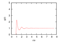
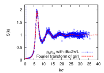
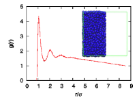
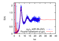
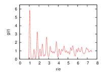
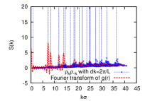
Figure 1: $g(r)$ (left) and $S(k)$ (right) for Lenard-Jones (of core size $\sigma$) liquid at density $\rho\sigma^{3}=0.8$ (top), lamellar phase at density $\rho\sigma^{3}=0.4$ (middle) and face-centered cubic crystal at density $\rho\sigma^{3}=1.2$. For $S(k)$ both direct calculation using Equation (2) (blue crosses) and Fourier transform of $g(r)$ using Equation (6) (red line) are shown.

References

• Hansen and McDonald (2013) J.Β Hansen and I.Β R. McDonald, Theory of Simple Liquids with Applications to Soft Matter (Academic Press, New York, 2013).
• foo (a) The Fourier transform convention sometimes takes the form of $\hat{\rho}_{\bf k}=\int\rho({\bf r})e^{-i{\bf k}\cdot{\bf r}}d{\bf r}$, which simply reverses the sign of the wavevector k.
• Allen and Tildesley (1987) M.Β P. Allen and D.Β J. Tildesley, Computer Simulation of Liquids (Oxford University Press, New York, 1987).
• foo (b) In some textbooks, the symbol $g(r)$ is used for the pair correlation function instead of $h(r)$.
• Chandler (1987) D.Β Chandler, Introduction to Modern Statistical Mechanics (Oxford University Press, New York, 1987).
• Gotze (2009) W.Β GΓΆtze, Complex Dynamics of Glass-Forming Liquids (Oxford University Press, Oxford, 2009).
• Barrat and Hansen (2003) J.Β Barrat and J.Β Hansen, Basic Concepts for Simple and Complex Liquids (Cambridge University Press, New York, 2003).
• McQuarrie (2000) D.Β A. McQuarrie, Statistical Mechanics (University Science Books, New York, 2000).
• Debenedetti (1996) P.Β G. Debenedetti, Metastable Liquids (Princeton University Press, Princeton, New Jersey, 1996).
• Wales (2003) D.Β J. Wales, Energy Landscapes with Applications to Clusters, Biomolecules and Glasses (Cambridge University Press, New York, 2003).
• foo (c) $\delta({\bf k})$ is the Dirac delta function and $\delta_{{\bf k},0}$ is the Kronecker delta function.
• foo (d) $S({\bf k})$ is singular at ${\bf k}=0$, i.e. $\lim\limits_{{\bf k}\to 0}S({\bf k})=1+\rho\lim\limits_{{\bf k}\to 0}\hat{h}_{\bf k}\neq 1+\rho\hat{h}_{0}+N=N=S(0)$, because lim𝐀→0δ𝐀,0=0β‰ 1=Ξ΄0,0subscript→𝐀0subscript𝛿𝐀001subscript𝛿00\lim\limits_{{\bf k}\to 0}\delta_{{\bf k},0}=0\neq 1=\delta_{0,0} and lim𝐀→0h^𝐀=ρ​kB​Tβ€‹ΞΊβˆ’Οβˆ’1β‰ βˆ’Οβˆ’1=h^0subscript→𝐀0subscript^β„Žπ€πœŒsubscriptπ‘˜π΅π‘‡πœ…superscript𝜌1superscript𝜌1subscript^β„Ž0\lim\limits_{{\bf k}\to 0}\hat{h}_{\bf k}=\rho k_{B}T\kappa-\rho^{-1}\neq-\rho^{-1}=\hat{h}_{0}.
• foo (d) Practically, the singularity of the $\delta({\bf k})$ function, which has an integral of 1 even being non-zero at one single point ${\bf k}=0$, makes the integration of $\hat{g}_{\bf k}$ (or $S({\bf k})$) from ${\bf k}=0$ poorly defined.