Guided Waves in Asymmetric Hyperbolic Slab Waveguides. The TM Mode Case

Abstract

Nonlinear guided wave modes in an asymmetric slab waveguide formed by an isotropic dielectric layer placed on a linear or nonlinear substrate and covered by a hyperbolic material are investigated. Optical axis is normal to the slab plane. The dispersion relations for TM waves are found. It is shown that there are additional cut-off frequencies for each TM mode. The effects of the nonlinearity on the dispersion relations are investigated and discussed. There are the modes, which are corresponded with situation where the peak of electric field is localized in the nonlinear substrate. These modes are absent in the linear waveguide. To excite these modes the power must exceed certain threshold value.

I Introduction

Hyperbolic metamaterials are artificially structured uniaxial materials with opposite signs of permittivity (or magnetic permeability) for ordinary and extraordinary waves Noginov:09 ; XNi:11 ; Drachev:13 ; Prashant:14 . The hyperbolic materials can be fabricated as a multilayer structure consisting of alternating metallic and dielectric layers Wood:06 ; Kivshar:13 ; Othman:13 , or as a nanowire structure consisting of metallic nanorods embedded in a dielectric host.

Due to the unusual hyperbolic form of the iso-frequency dispersion surfaces unlimited high values of the wave vector are possible in such materials. It results in the numerous effects, among which are the Purcell enhancement of the spontaneous emission rate in hyperbolic metamaterials Poddubny:12 ; Poddubny:13 ; Ward:13 ; Ferrari:14 and the subwavelength resolution effect Wood:06 ; Benedict:13 . The optical phenomena on the interface between conventional dielectric and hyperbolic metamaterial has also attracted attention. The surface waves were studied in Zapata:13 . The extremely large Goos -Hänchen shift has been studied in some details in JingZhao:13 .

The linear plasmonic planar waveguide cladded by hyperbolic metamaterials was proposed and investigated in Kildishev:14 ; Kildishev:15 . The linear guided waves properties of such hyperbolic slab waveguide were discussed in Lyashko:15 . It was shown that for the TM wave number of guided modes is limited. Each of these modes have two cut-off frequencies. One of them corresponds to the mode appearance, another corresponds to the mode disappearance. There is region of parameters in which only single mode exists in this waveguide. It is worth noting that this phenomenon is unavailable in the case of a conventional waveguide. Usually the number of modes increases with core thickness or radiation frequency, and only single cut-off frequency exists for each mode.

The purpose of this paper is to investigate the dispersion properties of the nonlinear guided waves in a planar asymmetric waveguide. It is assumed that linear isotropic film (i.e., core of waveguide) is placed on a nonlinear substrate. The core of waveguide is covered by the linear hyperbolic material. The anisotropy axis of the cladding layer is normal to the interface between core and surroundings. In the planar geometry, as is known Hansperger:84 , guided waves can be separated into two gropes of waves, which have a different polarization. These waves are referred to as TE and TM waves. In general case the nonlinear polarization entangles the TE and TM waves. The simplest case where only TM kind of the wave is exited will be considered.

The electric and magnetic field distributions and the dispersion relations will be found for the slab waveguide under consideration. If the extra-ordinary permittivity is less then a permittivity of core of waveguide, each TM mode of the hyperbolic waveguide both in the linear and nonlinear cases has an additional cut-off frequency and a transition point. Both the cut-off frequency and the transition point depend on power that is transferred by guided wave. If power exceeds a certain critical value, for each wave mode appears additional solution branch. The guiding waves, that correspond to these branches, differ in transverse configuration of field.

II Constituent equations

Let us consider the uniaxial anisotropic dielectric material. The vector $\mathbf{a}$ is the unit vector of an optical axis. In this case the Fourier component of the vector of dielectric displacement $\mathbf{D}$ can be written as

$$\mathbf{D}=\varepsilon_{o}\mathbf{E}+(\varepsilon_{e}-\varepsilon_{o})(\mathbf{a}\cdot\mathbf{E})\mathbf{a}+4\pi\mathbf{P}_{nl},$$

where $\mathbf{E}=\mathbf{E}(\mathbf{r},\omega)$ is the Fourier component of the electric field, $\varepsilon_{o}$ is an ordinary permittivity, and $\varepsilon_{e}$ is an extra-ordinary permittivity. Theses values are the linear principal dielectric constants for anisotropic material. Nonlinear properties of the material is defined by the nonlinear polarization vector $\mathbf{P}_{nl}$.

The Fourier component of the electric field $\mathbf{E}(\omega,\mathbf{r})$ in a nonmagnetic medium is governed by the following wave equation

$$\left(\nabla^{2}+k_{0}^{2}\varepsilon_{o}\right)\mathbf{E}+\frac{\Delta\varepsilon}{\varepsilon_{o}}\left[(\mathbf{a}\cdot\nabla)\nabla+k_{0}^{2}\varepsilon_{o}\mathbf{a}\right](\mathbf{a}\cdot\mathbf{E})+4\pi k_{0}^{2}\mathbf{P}_{nl}=0,$$ (1)

where $k_{0}=\omega/c$, $\Delta\varepsilon=\varepsilon_{e}-\varepsilon_{o}$. In the case of isotropic medium this equation is reduced to usual wave equation.

Let us consider a slab waveguide. We assume, that the material of the film (waveguide core) is nonmagnetic $\mu_{2}=1$ and has an isotropic permittivity $\varepsilon_{2}$. The film thickness is $h$. The dielectric film is placed on a linear or nonlinear substrate and covered by the uniaxial hyperbolic metamaterial which is characterized by symmetric dielectric tensor with the principal dielectric constants $\varepsilon_{o}$, and $\varepsilon_{e}$, and the magnetic permeability $\mu_{1}=1$. The anisotropy axis is aligned with a unit normal vector to the interface, i.e., along the $OX$ direction. Axes $OY$ and $OZ$ are parallel to the interface. Axis $OZ$ is directed along the wave propagation. In this case the Maxwell equations are invariant under the shifting along $OY$ axis. Thus, the strengths of electric and magnetic fields of the guided wave are independent on variable $y$. From it follows, that the wave equation (1) is splitting into two independent systems of equations describing the TE and TM waves

$$\left(\frac{\varepsilon_{e}(x)}{\varepsilon_{o}(x)}\frac{\partial^{2}}{\partial x^{2}}+\frac{\partial^{2}}{\partial z^{2}}+k_{0}^{2}\varepsilon_{e}(x)\right)E_{x}+4\pi k_{0}^{2}P_{nl,x}=0,$$

$$\left(\frac{\partial^{2}}{\partial x^{2}}+\frac{\partial^{2}}{\partial z^{2}}+k_{0}^{2}\varepsilon_{o}(x)\right)E_{y}+4\pi k_{0}^{2}P_{nl,y}=0,$$ (2)

$$\left(\frac{\partial^{2}}{\partial x^{2}}+\frac{\partial^{2}}{\partial z^{2}}+k_{0}^{2}\varepsilon_{o}(x)\right)E_{z}+\frac{\Delta\varepsilon(x)}{\varepsilon_{o}(x)}\frac{\partial^{2}}{\partial x\partial z}E_{x}+4\pi k_{0}^{2}P_{nl,z}=0.$$

The simple model of nonlinear medium will be considered Mihalache:86 ; Agranowich:86 . It what follows we will assumed that

$$\mathbf{P}_{nl}=\varepsilon_{K}(|E_{y}|^{2}+|E_{z}|^{2})\mathbf{E}$$ (3)

The TE wave is defined by the following electric and magnetic vectors $\mathbf{E}=(0,E_{y},0)$ and $\mathbf{H}=(H_{x},0,H_{z})$. Hence, the wave equation for $E_{y}$ from (2) can be used to describe the nonlinear wave propagation in this slab waveguide. TE wave is the ordinary wave and the new results in this case are not expected.

The electric and magnetic vectors of the TM wave are $\mathbf{E}=(E_{x},0,E_{z})$ and $\mathbf{H}=(0,H_{y},0)$.

The components of these vectors are related by the Maxwell equations, that are

$$\qquad\qquad\qquad H_{y}=\frac{i}{k_{0}}\left(\frac{\partial E_{z}}{\partial x}-\frac{\partial E_{x}}{\partial z}\right),$$ (4)

$$\frac{\partial H_{y}}{\partial z}=ik_{0}\varepsilon_{e}(x)E_{x}+4\pi ik_{0}P_{nl,x},\quad\frac{\partial H_{y}}{\partial x}=-ik_{0}\varepsilon_{o}(x)E_{z}-ik_{0}4\pi P_{nl,z}.$$ (5)

The linear principal dielectric constants are piecewise functions :

$$\varepsilon_{o}(x)=\left\{\begin{array}[]{ccc}\varepsilon_{1}&x<0,\\ \varepsilon_{2}&0\leq x\leq h,\\ \varepsilon_{o}&x>h,\\ \end{array}\right.\quad\varepsilon_{e}(x)=\left\{\begin{array}[]{ccc}\varepsilon_{1}&x<0,\\ \varepsilon_{2}&0\leq x\leq h,\\ \varepsilon_{e}&x>h,\\ \end{array}\right.$$ (6)

III Linear slab waveguide

III.1 Electromagnetic field distributions

As the waveguide is homogeneous medium along the axis $OZ$, the electric and magnetic vectors of the TM wave can be represented by the following expressions: $\mathbf{E}=(\tilde{E}_{x},0,\tilde{E}_{z})e^{i\beta z}$ and $\mathbf{H}=(0,\tilde{H}_{y},0)e^{i\beta z}$, where $\beta$ is propagation constant Hansperger:84 . From the system of equations (2) the equations for $\tilde{E}_{z}$ result in

$$x<0 \frac{\partial^{2}}{\partial x^{2}}\tilde{E}_{z}+(k_{0}^{2}\varepsilon_{1}-\beta^{2})\tilde{E}_{z}=0,$$

$$0\leq x\leq h \frac{\partial^{2}}{\partial x^{2}}\tilde{E}_{z}+(k_{0}^{2}\varepsilon_{2}-\beta^{2})\tilde{E}_{z}=0,$$ (7)

$$x>h \frac{\partial^{2}}{\partial x^{2}}\tilde{E}_{z}+\frac{\varepsilon_{o}}{\varepsilon_{e}}(k_{0}^{2}\varepsilon_{e}-\beta^{2})\tilde{E}_{z}=0,$$

The solutions of these equations with taking into account the boundary conditions at $x\to\pm\infty$ (i.e.,outside of waveguide all fields are disappeared) $\tilde{E}_{z}(x)$ and magnetic field distributions $\tilde{H}_{y}(x)$ are

$$x<0 \tilde{E}^{(1)}_{z}(x)=A_{0}e^{px},\qquad\qquad\qquad\tilde{H}^{(1)}_{y}=-\frac{ik_{0}\varepsilon_{1}}{p}A_{0}e^{px},$$ (8)

$$0\leq x\leq h \tilde{E}^{(2)}_{z}(x)=B_{1}e^{i\kappa x}+B_{2}e^{-i\kappa x},\quad\tilde{H}^{(2)}_{y}(x)=-\frac{k_{0}\varepsilon_{2}}{\kappa}\left(B_{1}e^{i\kappa x}-B_{2}e^{-i\kappa x}\right),$$ (9)

$$x>h \tilde{E}^{(3)}_{z}(x)=Ce^{-qx},\qquad\qquad\qquad\tilde{H}^{(3)}_{y}(x)=\frac{ik_{0}\varepsilon_{o}}{q}Ce^{-qx},$$ (10)

where the real positive value

$$p=\sqrt{\beta^{2}-k_{0}^{2}\varepsilon_{1}},\quad q=\sqrt{\varepsilon_{o}/\varepsilon_{e}(\beta^{2}-k_{0}^{2}\varepsilon_{e}}),\quad\kappa=\sqrt{k_{0}^{2}\varepsilon_{2}-\beta^{2}},$$

are introduced. If the $\kappa$ is imaginary value then the solutions (8)–(10) describe the coupled surface wave propagation.

The electromagnetic field is confined in waveguide if the conditions

$$k_{0}^{2}\varepsilon_{1}<\beta^{2}<k_{0}^{2}\varepsilon_{2},\quad(\varepsilon_{o}/\varepsilon_{e})(\beta^{2}-k_{0}^{2}\varepsilon_{e})>0$$

are held. In the case of hyperbolic material with $\varepsilon_{o}>0$, $\varepsilon_{e}<0$ the second inequality breaks down for any $\beta$. The evanescent wave comes into covering layer. Oppositely, in the case of hyperbolic material with $\varepsilon_{o}<0$, $\varepsilon_{e}>0$ the second inequality can be held, if $\beta^{2}<k_{0}^{2}\varepsilon_{e}$. Let us introduce the effective index $n_{eff}=\beta/k_{0}$. Thus the confinement condition reads as

$$\varepsilon_{1}<n_{eff}^{2}<\min(\varepsilon_{e},~{}\varepsilon_{2}).$$ (11)

The continuity conditions for tangent components of both electric and magnetic field vectors at $x=0$ and $x=h$ result in following relations:

$$A_{0}=B_{1}+B_{2},\qquad\frac{i\varepsilon_{1}}{p}A_{0}=\frac{\varepsilon_{2}}{\kappa}(B_{1}-B_{2}),$$

$$Ce^{-qh}=B_{1}e^{i\kappa h}+B_{2}e^{-i\kappa h},$$ (12)

$$\frac{i\varepsilon_{o}}{q}Ce^{-qh}=-\frac{\varepsilon_{2}}{\kappa}\left(B_{1}e^{i\kappa h}-B_{2}e^{-i\kappa h}\right).$$

From the first and second equations of this system of the linear equations follows that

$$B_{1}=\frac{A_{0}}{2}\left(1+i\frac{\varepsilon_{1}\kappa}{\varepsilon_{2}p}\right),\quad B_{2}=\frac{A_{0}}{2}\left(1-i\frac{\varepsilon_{1}\kappa}{\varepsilon_{2}p}\right).$$

Amplitude $C$ is

$$C=\frac{1}{2}\left[\left(1+i\frac{\varepsilon_{1}\kappa}{\varepsilon_{2}p}\right)e^{i\kappa h}+\left(1-i\frac{\varepsilon_{1}\kappa}{\varepsilon_{2}p}\right)e^{-i\kappa h}\right]A_{0}e^{qh}.$$

Thus the electric field distribution of the TM wave can be written as

$$x<0 \tilde{E}^{(1)}_{z}(x)=A_{0}e^{px},$$

$$0\leq x\leq h \tilde{E}^{(2)}_{z}(x)=A_{0}\left(\cos(\kappa x)-\frac{\varepsilon_{1}\kappa}{\varepsilon_{2}p}\sin(\kappa x)\right),$$ (13)

$$x>h \tilde{E}^{(3)}_{z}(x)=A_{0}\left(\cos(\kappa h)-\frac{\varepsilon_{1}\kappa}{\varepsilon_{2}p}\sin(\kappa h)\right)e^{-q(x-h)},$$

III.2 Dispersion relation

The dispersion relation for the localized in the waveguide electromagnetic waves represents the relationship between a propagation constant $\beta$ and a frequency $\omega$. The dispersion relations for the guided waves under consideration can be determined using the continuity conditions of an electric and magnetic field on interferences, as was done in Lyashko:15 . The linear system of algebraic equations (12) has non-zero solutions if the determinant of this system is zero. This claim results in the desired dispersion relation. As a consequence the following expression can be found

$$e^{2i\kappa h}\left(\frac{1-i\xi_{p}}{1+i\xi_{p}}\right)\left(\frac{1+i\xi_{q}}{1-i\xi_{q}}\right)=1,$$ (14)

where following parameters

$$\xi_{p}=\frac{\varepsilon_{2}p}{\varepsilon_{1}\kappa},\quad\xi_{q}=\frac{\varepsilon_{2}q}{|\varepsilon_{o}|\kappa}$$

are used. The Goos- Hänchen phase shifts $\phi_{q}$ and $\phi_{p}$ are defined by following expressions $\xi_{q}=-\tan(\phi_{q}/2)$ and $\xi_{p}=\tan(\phi_{p}/2)$. Using these expressions we can write the dispersion relation in form

$$2\kappa h-\phi_{p}-\phi_{q}=2\pi m,\quad m=0,~{}1,~{}2,\ldots$$ (15)

If the effective index of refraction $n_{eff}$ is used, than equation (15) can be written as

$$k_{0}h\sqrt{\varepsilon_{2}-n_{eff}^{2}}=\arctan\left(\frac{\varepsilon_{2}}{\varepsilon_{1}}\sqrt{\frac{n_{eff}^{2}-\varepsilon_{1}}{\varepsilon_{2}-n_{eff}^{2}}}\right)-\arctan\left(\frac{\varepsilon_{2}}{\sqrt{\varepsilon_{e}|\varepsilon_{o}|}}\sqrt{\frac{\varepsilon_{e}-n_{eff}^{2}}{\varepsilon_{2}-n_{eff}^{2}}}\right)+\pi m.$$ (16)

Thus the dispersion relation as the implicit function $n_{eff}$ of the $\varepsilon_{1}$, $\varepsilon_{2}$, $\varepsilon_{e}$, $h$, $\omega=ck_{0}$ is obtained.

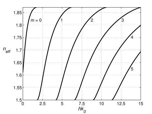
Figure 1: Dispersion curves for TM modes of the hyperbolic waveguide. $\varepsilon_{e}<\varepsilon_{2}$ .

Let it be $\varepsilon_{e}<\varepsilon_{2}$. In this case the two cut-off frequencies series take place. At $n_{eff}^{2}=\varepsilon_{1}$ they are $V_{cm}^{(1)}$, and at $n_{eff}^{2}=\varepsilon_{e}$ they are $V_{cm}^{(2)}$, where

$$V_{cm}^{(1)}=k_{0}h\sqrt{\varepsilon_{2}-\varepsilon_{1}} = \pi m-\arctan\left(\frac{\varepsilon_{2}}{\sqrt{\varepsilon_{e}|\varepsilon_{o}|}}\sqrt{\frac{\varepsilon_{e}-\varepsilon_{1}}{\varepsilon_{2}-\varepsilon_{1}}}\right),$$ (17)

$$V_{cm}^{(2)}=k_{0}h\sqrt{\varepsilon_{2}-\varepsilon_{e}} = \pi m+\arctan\left(\frac{\varepsilon_{2}}{\varepsilon_{1}}\sqrt{\frac{\varepsilon_{e}-\varepsilon_{1}}{\varepsilon_{2}-\varepsilon_{e}}}\right).$$ (18)

As the wavenumber $k_{0}$ depends on the frequency of radiation, the waveguide guides every TM mode only in certain frequency range.

It should be pointed that $V_{c0}^{(1)}$ is negative quantity, that is impossible. Hence, the dispersion curve with $m=0$ presents the special situation. At $m=0$ the dispersion relation is

$$k_{0}h\sqrt{\varepsilon_{2}-n_{eff}^{2}}=\arctan\left(\frac{\varepsilon_{2}}{\varepsilon_{1}}\sqrt{\frac{n_{eff}^{2}-\varepsilon_{1}}{\varepsilon_{2}-n_{eff}^{2}}}\right)-\arctan\left(\frac{\varepsilon_{2}}{\sqrt{\varepsilon_{e}|\varepsilon_{o}|}}\sqrt{\frac{\varepsilon_{e}-n_{eff}^{2}}{\varepsilon_{2}-n_{eff}^{2}}}\right).$$

As the left-hand side of this expression is positive one, then on the right-hand side the sum of terms is positive too. It results in

$$\frac{n_{eff}^{2}-\varepsilon_{1}}{\varepsilon_{1}^{2}}\geq\frac{\varepsilon_{e}-n_{eff}^{2}}{\varepsilon_{e}|\varepsilon_{o}|}.$$

Hence, the minimal effective index of this dispersion curve with $m=0$ is determined by equation

$$\min n_{eff}^{2}=\varepsilon_{1}+\frac{\varepsilon_{1}^{2}(\varepsilon_{e}-\varepsilon_{1})}{\varepsilon_{1}^{2}+\varepsilon_{e}|\varepsilon_{o}|}.$$

It should be remarked that this magnitude of effective index is achieved at the zero film thickness. In the case of a conventional asymmetrical slab waveguide the cut-off frequencies corresponding $m=0$ is positive quantity. The property of the guided mode with $m=0$ discussed above is the feature of hyperbolic asymmetrical slab waveguide.

If the zigzag-ray model for light propagation in slab waveguide Kogelnik:Weber:74 is used, then effective index can be represented by the formula $n_{eff}=\sqrt{\varepsilon_{2}}\sin\alpha$, where $\alpha$ is the incident angle on the film-substrate and film-cover interfaces. The inequality (11) results in

$$\frac{\varepsilon_{1}}{\varepsilon_{2}}<\sin^{2}\alpha<\min\left(\frac{\varepsilon_{e}}{\varepsilon_{2}}~{},1\right).$$ (19)

When $\varepsilon_{2}<\varepsilon_{e}$ inequality (19) is consistent with the usual condition for dielectric waveguides. The light ray is totally reflected at the film-substrate interface if $\alpha>\alpha_{1}=\arcsin(\varepsilon_{1}/\varepsilon_{2})^{1/2}$. If $\varepsilon_{2}>\varepsilon_{e}$, the second critical angle occurs. Now the confinement condition reads as $\alpha_{1}<\alpha<\alpha_{2}$, where $\alpha_{2}=\arcsin(\varepsilon_{e}/\varepsilon_{2})^{1/2}$. It means that the two cut-off frequencies take place in the hyperbolic waveguide under consideration. Fig.1 shows the branches of dispersion curves ($m=0\div 5$) on condition that $\varepsilon_{1}=2.25$, $\varepsilon_{2}=4.0$, $\varepsilon_{e}=3.5$, and $\varepsilon_{o}=-3.85$.

Now let it be $\varepsilon_{e}>\varepsilon_{2}$. In this case only one cut-off frequencies series takes place: $V_{cm}^{(1)}$, $m\geq 1$, which is determined by equation (17). At $m=0$ guided mode has the properties identical to that for the case of $\varepsilon_{e}<\varepsilon_{2}$.

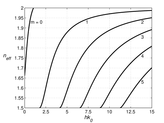
Figure 2: Dispersion curves for TM modes of the hyperbolic waveguide. $\varepsilon_{e}<\varepsilon_{2}$ .

The dispersion curves at $m=0\div 5$ on condition that $\varepsilon_{1}=2.25$, $\varepsilon_{2}=4.0$, $\varepsilon_{e}=4.5$, and $\varepsilon_{o}=-3.85$ are shown in Fig.2. One can see that the cut-off frequencies $V_{cm}^{(2)}$ with $m\geq 1$ are lacking. However mode with $m=0$ has the second cut-off frequency.

IV Nonlinear waveguide

Now the effect of nonlinearity will be considered. Nonlinear property of the substrate will be described using the (3) Agranowich:86 . As the electric field vector of the considered TM waves is $\mathbf{E}=(E_{x},0,E_{z})$, the nonlinear polarization $P_{z,nl}$ can be written as

$$P_{z,nl}=\varepsilon_{K}|E_{z}|^{2}E_{z}.$$ (20)

Electric field distributions are governed by following equations

$$x<0 \frac{\partial^{2}}{\partial x^{2}}\tilde{E}_{z}+(k_{0}^{2}\varepsilon_{1}-\beta^{2})\tilde{E}_{z}+k_{0}^{2}\varepsilon_{K}\tilde{E}_{z}^{3}=0,$$

$$0\leq x\leq h \frac{\partial^{2}}{\partial x^{2}}\tilde{E}_{z}+(k_{0}^{2}\varepsilon_{2}-\beta^{2})\tilde{E}_{z}=0,$$ (21)

$$x>h \frac{\partial^{2}}{\partial x^{2}}\tilde{E}_{z}+\frac{\varepsilon_{o}}{\varepsilon_{e}}(k_{0}^{2}\varepsilon_{e}-\beta^{2})\tilde{E}_{z}=0,$$

The normal component of the electric field and the tangent component of magnetic field distribution can be obtained from the following expression

$$\tilde{H}_{y}(x)=\frac{ik_{0}\varepsilon_{e}(x)}{k_{0}^{2}\varepsilon_{e}(x)-\beta^{2}}\frac{\partial\tilde{E}_{z}}{\partial x},\qquad\tilde{E}_{x}(x)=\frac{i\beta}{k_{0}^{2}\varepsilon_{e}(x)-\beta^{2}}\frac{\partial\tilde{E}_{z}}{\partial x}.$$

The permittivity function $\varepsilon_{e}(x)$ is defined by the expression (6).

IV.1 Electromagnetic field distributions

As above the the real positive parameters $p=\sqrt{\beta^{2}-k_{0}^{2}\varepsilon_{1}}$,  $q=\sqrt{\varepsilon_{o}/\varepsilon_{e}(\beta^{2}-k_{0}^{2}\varepsilon_{e}})$, and $\kappa=\sqrt{k_{0}^{2}\varepsilon_{2}-\beta^{2}}$ are introduced. The electric fields in dielectric film and hyperbolic cover have already been found, eqs. (9) and (10). Electric field distribution in nonlinear substrate is governed by the first equation of system (21). Solution of this equation can be written as

$$\tilde{E}_{z}^{(1)} = \sqrt{\frac{2p^{2}}{k_{0}^{2}\varepsilon_{K}}}\frac{1}{\cosh[p(x-x_{0})]},\quad\varepsilon_{K}>0,$$ (22)

$$\tilde{E}_{z}^{(1)} = \sqrt{\frac{2p^{2}}{k_{0}^{2}|\varepsilon_{K}|}}\frac{1}{\sinh[p(x-x_{0})]},\quad\varepsilon_{K}<0,$$ (23)

The parameter $x_{0}$ dictates the location of the electric field maximum. In the case of $\varepsilon_{K}<0$ the function in (23) tends to infinity at $x_{0}>0$. So only the case $x_{0}>0$ when special point lyes outside of nonlinear medium is possible. Hence the electric field maximum is located at $x=0$. In the case of $\varepsilon_{K}>0$ one can find that $x_{0}<0$ (the electric field maximum is located in nonlinear substrate) or $x_{0}>0$ (the electric field maximum is located at $x=0$). Furthermore we will consider only the case of $\varepsilon_{K}>0$.

The useful parameters are the electric field amplitude at the boundary of nonlinear substrate $\tilde{A}_{0}=\tilde{E}_{z}^{(1)}(x=0)$ and the measure of nonlinearity $\nu$:

$$\tilde{A}_{0}=\sqrt{\frac{2p^{2}}{k_{0}^{2}\varepsilon_{K}}}\frac{1}{\cosh(px_{0})}=\frac{A_{m}}{\cosh(px_{0})},\quad\nu=\tanh(px_{0})=\mathrm{sgn}(x_{0})\left(1-\frac{k_{0}^{2}\varepsilon_{K}}{2p^{2}}\tilde{A}_{0}^{2}\right)^{1/2}.$$

It should be pointed that $\tilde{A}_{0}$ is limited: $\tilde{A}_{0}^{2}\leq 2p^{2}/k_{0}^{2}\varepsilon_{K}$. $A_{m}$ is the peak of the electric field in substrate. The positive sign of $\nu$ correlates with monotonic behavior of the electric field, the negative sign of $\nu$ correlates with the localization of the electric field maximum in nonlinear substrate (see Fig. 3).

With these parameters the expression (22) can be rewritten as

$$\tilde{E}_{z}^{(1)}(x)=\frac{A_{m}}{\cosh[(px-x_{0})]}=\frac{\tilde{A}_{0}}{\cosh(px)-\nu\sinh(px)}.$$ (24)

The function describing the electric fields in linear media $\tilde{E}_{z}^{(2)}(x)$ and $\tilde{E}_{z}^{(3)}(x)$ were found above.

The magnetic field distributions are

$$x<0 \tilde{H}^{(1)}_{y}(x)=\frac{ik_{0}\varepsilon_{1}A_{m}\tanh[p(x-x_{0})]}{p\cosh[p(x-x_{0})]},$$

$$0\leq x\leq h \tilde{H}^{(2)}_{y}(x)=-\frac{k_{0}\varepsilon_{2}}{\kappa}\left(B_{1}e^{i\kappa x}-B_{2}e^{-i\kappa x}\right),$$ (25)

$$x>h \tilde{H}^{(3)}_{y}(x)=\frac{ik_{0}\varepsilon_{o}}{q}Ce^{-qx}.$$

The continuity conditions for tangent components of the electric and the magnetic field vectors at $x=0$ and $x=h$ involve the following relations

$$\tilde{A}_{0}=B_{1}+B_{2},\qquad\frac{i\varepsilon_{1}}{\tilde{p}}\tilde{A}_{0}=\frac{\varepsilon_{2}}{\kappa}(B_{1}-B_{2}),$$ (26)

$$Ce^{-qh}=B_{1}e^{i\kappa h}+B_{2}e^{-i\kappa h},$$ (27)

$$\frac{\varepsilon_{o}}{iq}Ce^{-qh}=\frac{\varepsilon_{2}}{\kappa}\left(B_{1}e^{i\kappa h}-B_{2}e^{-i\kappa h}\right),$$ (28)

where $\tilde{p}=p/\nu$.

The equations (26) and (27) allow one to find the electric field distributions

$$x<0 \tilde{E}^{(1)}_{z}(x)=\frac{\tilde{A}_{0}\cosh(px_{0})}{\cosh[p(x-x_{0})]},$$

$$0\leq x\leq h \tilde{E}^{(2)}_{z}(x)=\tilde{A}_{0}\left(\cos(\kappa x)-\nu\frac{\varepsilon_{1}\kappa}{\varepsilon_{2}p}\sin(\kappa x)\right),$$ (29)

$$x>h \tilde{E}^{(3)}_{z}(x)=\tilde{A}_{0}\left(\cos(\kappa h)-\nu\frac{\varepsilon_{1}\kappa}{\varepsilon_{2}p}\sin(\kappa h)\right)e^{-q(x-h)}.$$

If $\nu\to 1$, then the results of the linear waveguide are reproduced.

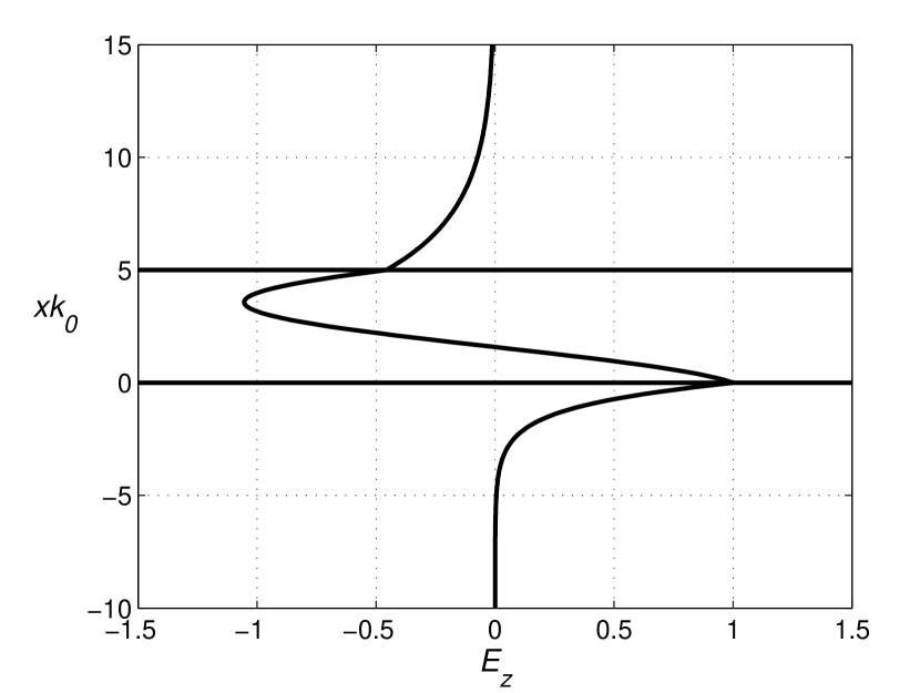
(a)

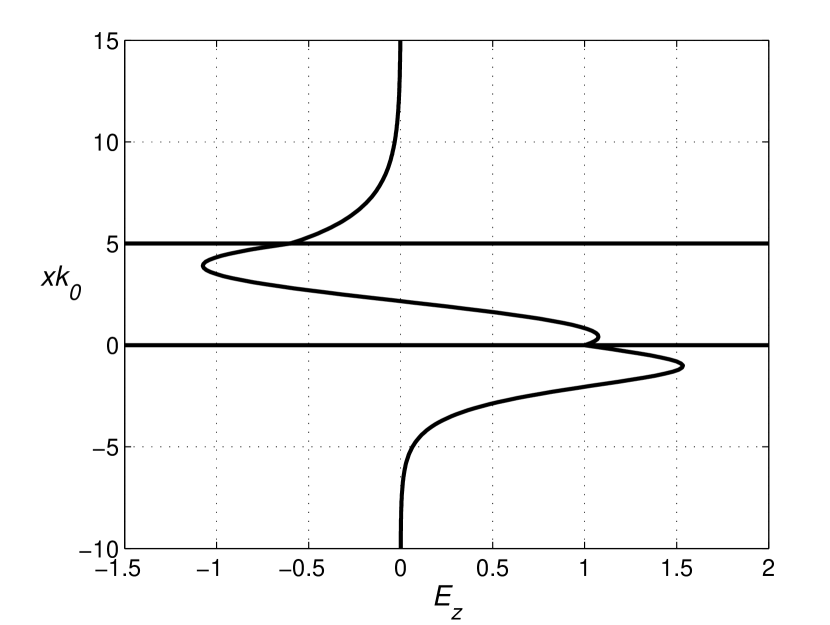
(b)

Figure 3: Transverse distribution of the electric field $\tilde{E}_{z}(x)$ at $m=1$. (a) $\nu>0$, (b) $\nu<0$.

IV.2 Dispersion relation

The dispersion relation for the guided TM wave in the slab waveguide under consideration results from the condition that the determinant of the system of linear equations (26)– (28) is equal to zero. It leads one to the following expression

$$k_{0}h\sqrt{\varepsilon_{2}-n_{eff}^{2}}=\arctan\left(\frac{\varepsilon_{2}}{\nu\varepsilon_{1}}\sqrt{\frac{n_{eff}^{2}-\varepsilon_{1}}{\varepsilon_{2}-n_{eff}^{2}}}\right)-\arctan\left(\frac{\varepsilon_{2}}{\sqrt{\varepsilon_{e}|\varepsilon_{o}|}}\sqrt{\frac{\varepsilon_{e}-n_{eff}^{2}}{\varepsilon_{2}-n_{eff}^{2}}}\right)+\pi m,$$ (30)

where the effective index $n_{eff}$ is used. By using the definition of parameter $\nu$ this expression can be rewritten as

$$k_{0}h\sqrt{\varepsilon_{2}-n_{eff}^{2}}=\mathrm{sgn}(\nu)\arctan\left(\frac{\varepsilon_{2}}{\varepsilon_{1}}\sqrt{\frac{(n_{eff}^{2}-\varepsilon_{1})^{2}}{(\varepsilon_{2}-n_{eff}^{2})(n_{eff}^{2}-\varepsilon_{nl})}}\right)-\arctan\left(\frac{\varepsilon_{2}}{\sqrt{\varepsilon_{e}|\varepsilon_{o}|}}\sqrt{\frac{\varepsilon_{e}-n_{eff}^{2}}{\varepsilon_{2}-n_{eff}^{2}}}\right)+\pi m,$$ (31)

where $\varepsilon_{nl}=\varepsilon_{1}+\varepsilon_{K}\tilde{A}_{0}^{2}/2$. $\mathrm{sgn}(\nu)$ corresponds to two branches of the dispersion relation. These $\nu$-branches each contain the series of the curves marked by integer $m$. At positive $\nu$ the expression (31) is reduced to the dispersion relation for linear guided waves (16) when $\nu\to 1$ or $\varepsilon_{K}\to 0$. The negative $\nu$ corresponds with situation where the peak of the electric field is localized in the nonlinear substrate. That is impossible in the linear waveguide case Stegeman:Seaton:85 ; Mihalache:86 ; Lederer:83b .

Dispersion relation (31) involves the inequality for effective index

$$\varepsilon_{nl}\leq n_{eff}^{2}<\min(\varepsilon_{e},~{}\varepsilon_{2}).$$ (32)

Comparison of the inequality (11) with (32) under taking into account definition of $\varepsilon_{nl}$ shows decreasing of the interval of relevant effective indexes.

At $n_{eff}^{2}=\varepsilon_{nl}$ expression (31) results in

$$k_{0}h\sqrt{\varepsilon_{2}-\varepsilon_{nl}}=\pi\left(m\pm\frac{1}{2}\right)-\arctan\left(\frac{\varepsilon_{2}}{\sqrt{\varepsilon_{e}|\varepsilon_{o}|}}\sqrt{\frac{\varepsilon_{e}-\varepsilon_{nl}}{\varepsilon_{2}-\varepsilon_{nl}}}\right).$$ (33)

Hence, the point $n_{eff}=\varepsilon_{nl}^{1/2}$ is the common one for both dispersion curve marked $m$ and dispersion curve with $m+1$. Therewith the dispersion curve marked $m$ belongs to positive $\nu$ branch, but the mode marked $m+1$ belongs to negative $\nu$ branch. Thus the points $n_{eff}=\varepsilon_{nl}^{1/2}$ connect the two $\nu$-branches of the dispersion curves. These points are referred to as the transition points Lederer:85 .

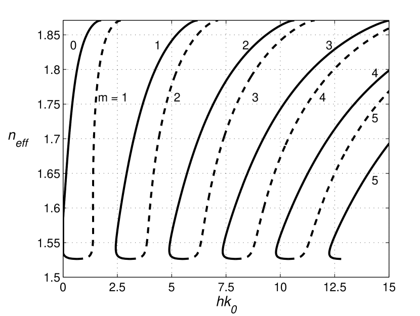
(a)

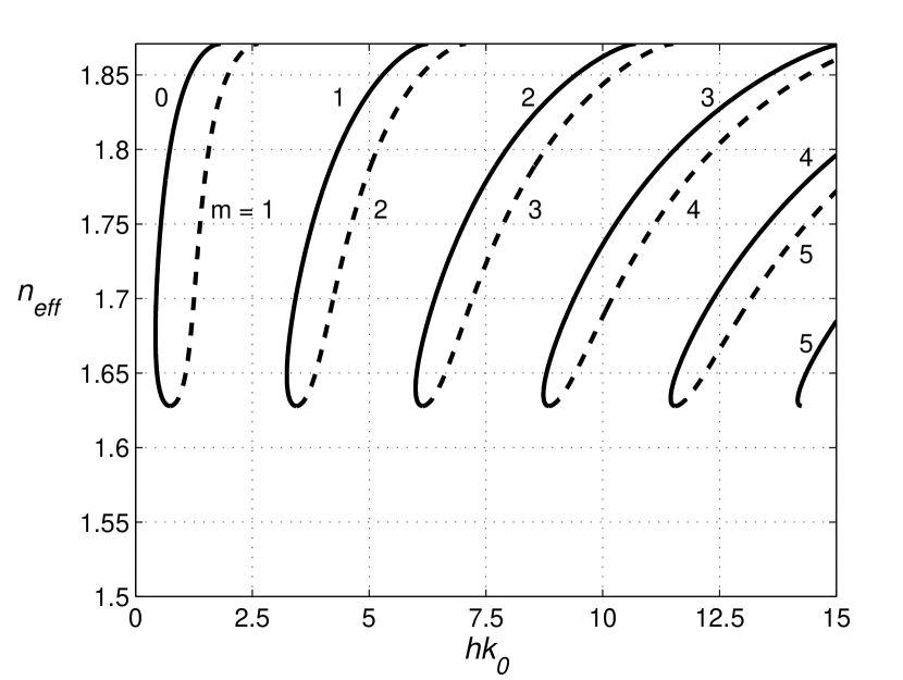
(b)

Figure 4: Dispersion curves for different value of $\varepsilon_{nl}$ and mode mark $m$. (a) $\varepsilon_{nl}=2.33$, (b) $\varepsilon_{nl}=2.65$.

The case of $\varepsilon_{2}>\varepsilon_{e}$ is considered. Fig. 4 shows the dispersion curves for different $\varepsilon_{nl}$ (i.e., for different values of $\tilde{A}_{0}^{2}$) at $\varepsilon_{1}=2.25$, $\varepsilon_{2}=4$, $\varepsilon_{e}=3.5$, $\varepsilon_{0}=-3.85$. Mode mark $m$ ranges from 0 to 5. Solid (dashed) curves correspond to $\nu>0$ ($\nu<0$). As the $k_{0}h$ increases, the electric field distribution is transformed, so that the electric field maximum is beginning to shift from film to substrate and it crosses the interface $x=0$ at transient point. It should be pointed that positive value of $x_{0}$ is the position of the virtual peak. Thus the real electric field maximum is located at $x=0$ as long as $k_{0}h$ does not achieve the transient point.

If $\varepsilon_{2}>\varepsilon_{e}$ then except for transition points (33) two series of the cut-off frequencies exists:

$$V_{cm}^{\pm}=k_{0}h\sqrt{\varepsilon_{2}-\varepsilon_{e}}=\pm\arctan\left(\frac{\varepsilon_{2}}{\varepsilon_{1}}\sqrt{\frac{(\varepsilon_{e}-\varepsilon_{1})^{2}}{(\varepsilon_{2}-\varepsilon_{e})(\varepsilon_{e}-\varepsilon_{nl})}}\right)+\pi m.$$ (34)

As in the case of the linear waveguide here the dispersion curves marked by $m=0$ represent the special case. If $\mathrm{sgn}(\nu)=-1$ then the curve with $m=0$ is absent. For $\mathrm{sgn}(\nu)=+1$ the cut-off frequency formally is negative. However, it means that minimum of the effective index is more then $\varepsilon_{nl}$ as previously. Minimum of the effective index can be written as $\min n_{eff}^{2}=\varepsilon_{nl}+\vartheta$, where $\vartheta$ is minimal root of the equation

$$\varepsilon_{e}|\varepsilon_{o}|(\vartheta+\varepsilon_{nl}-\varepsilon_{1})^{2}=\varepsilon_{1}^{2}\vartheta(\varepsilon_{e}-\varepsilon_{1}-\vartheta),$$

Let us denote intensity parameter $a_{nl}$ as difference $\varepsilon_{nl}-\varepsilon_{1}$. Fig. 5 presents the cut-off frequencies $V_{cm}^{\pm}$ on the intensity parameter. Solid (dashed) curve shows behavior of $V_{cm}^{+}$ ($V_{cm}^{-}$) for $\nu>0(\nu<0$). On this figure $k_{0}h$ corresponding with the cut-off frequencies are indicated. In the limit $a_{nl}=p^{2}/k_{0}^{2}$, where $\nu=0$, curves of the different $\nu$-branch converge to a common point. This convergence therewith takes place for the curves with ($\nu>0$, $m$) and ($\nu<0$, $m+1$).

The curves in the Fig. 5 demonstrate a weak dependence of the cut-off frequencies on intensity parameter. The frequency corresponding to a transition point essentially depends on the intensity parameter (Fig.6).

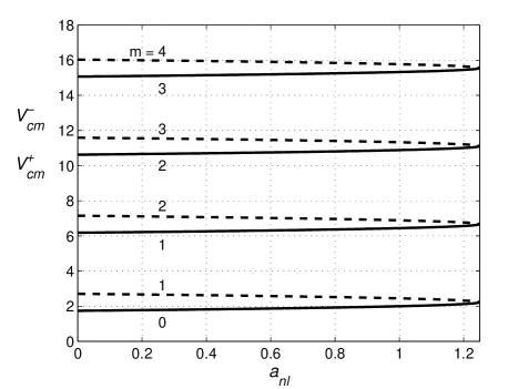
Figure 5: Cut-off frequencies $V_{cm}^{\pm}/\sqrt{\varepsilon_{2}-\varepsilon_{e}}$ as function of intensity parameter $a_{nl}$ at some mode mark $m$.

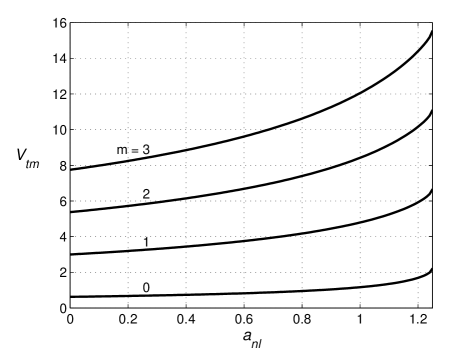
Figure 6: Dependence of the transition point position on intensity parameter $a_{nl}$ at some mode mark $m$.

The case of $\varepsilon_{2}>\varepsilon_{e}$ is considered. Fig.7 shows the dispersion curves for different $\varepsilon_{nl}$ at $\varepsilon_{1}=2.25$, $\varepsilon_{2}=4$, $\varepsilon_{e}=4.5$, $\varepsilon_{0}=-3.85$. Mode mark $m$ ranges from 0 to 5. Solid (dashed) curves correspond to $\nu>0$ ($\nu<0$). The cut-off frequencies $V_{cm}^{\pm}$ can be defined only for the curve with marker $m=0$ from branch with $\nu>0$ and the curve marked $m=1$ from branch with $\nu<0$. The transition points exist for all curves.

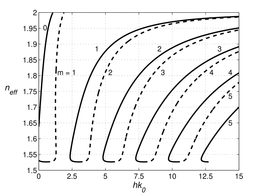
(a)

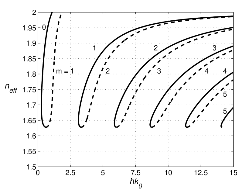
(b)

Figure 7: Dispersion curves for different value of $\varepsilon_{nl}$ and mode mark $m$ at condition $\varepsilon_{2}<\varepsilon_{e}$. (a) $\varepsilon_{nl}=2.33$, (b) $\varepsilon_{nl}=2.65$.

V Power fluxes in the nonlinear hyperbolic waveguide

The Poynting vector defines density of the radiation energy flux and direction of wave’s energy propagation. It is instructive to consider an averaged projection of the Poynting vector along the $OZ$ axis:

$$\langle S_{z}\rangle=\frac{c}{16\pi}(E_{x}^{*}H_{y}+E_{x}H_{y}^{*}).$$ (35)

The relation (35) can be rewritten with taking into account the Maxwell equation for TM wave and the power can be written as

$$P_{z}=\frac{c}{8\pi}\int_{-\infty}^{+\infty}\frac{n_{eff}}{\varepsilon_{e}(x)}|\tilde{H}_{y}(x)|^{2}dx.$$ (36)

Tangential components of the magnetic field distributions $\tilde{H}_{y}$ are represented by the following expressions:

$$x<0 \tilde{H}^{(1)}_{y}(x)=\frac{ik_{0}\varepsilon_{1}\tilde{A}_{0}\cosh(px_{0})}{p}\frac{\tanh[p(x-x_{0})]}{\cosh[p(x-x_{0})]},$$

$$0\leq x\leq h \tilde{H}^{(2)}_{y}(x)=-\frac{ik_{0}\varepsilon_{2}\tilde{A}_{0}}{\kappa}\left(\sin(\kappa x)+\nu\frac{\varepsilon_{1}\kappa}{\varepsilon_{2}p}\cos(\kappa x)\right),$$ (37)

$$x>h \tilde{H}^{(3)}_{y}(x)=\frac{ik_{0}\varepsilon_{o}\tilde{A}_{0}}{q}\left(\cos(\kappa h)-\nu\frac{\varepsilon_{1}\kappa}{\varepsilon_{2}p}\sin(\kappa h)\right)e^{-q(x-h)}.$$

Total power flux $P_{z}$ is equal to sum of the power flux in the substrate $P_{z}^{(1)}$, the power flux in the dielectric core $P_{z}^{(2)}$ and the power flux in the hyperbolic material covering the dielectric layer $P_{z}^{(3)}$. These values are calculating as

$$P_{z}^{(1)}=\frac{cn_{eff}}{8\pi\varepsilon_{1}}\int_{-\infty}^{0}|\tilde{H}^{(1)}_{y}(x)|^{2}dx,\quad P_{z}^{(2)}=\frac{cn_{eff}}{8\pi\varepsilon_{2}}\int_{0}^{h}|\tilde{H}^{(2)}_{y}(x)|^{2}dx,\quad P_{z}^{(3)}=\frac{cn_{eff}}{8\pi\varepsilon_{e}}\int_{h}^{+\infty}|\tilde{H}^{(3)}_{y}(x)|^{2}dx.$$

Using the equations (25) these partial values of the power flux can be determined:

$$P_{z}^{(1)}=\frac{c}{24\pi}\frac{k_{0}^{2}n_{eff}\varepsilon_{1}}{p^{3}}A_{0}^{2}\left(\cosh^{2}(px_{0})-\nu\sinh^{2}(px_{0})\right),$$

$$P_{z}^{(2)}=\frac{c}{16\pi}\frac{k_{0}^{2}n_{eff}\varepsilon_{2}}{\kappa^{3}}A_{0}^{2}\left[\kappa h\left(1+\frac{\nu^{2}}{\xi_{p}^{2}}\right)-\frac{1}{2}\left(1-\frac{\nu^{2}}{\xi_{p}^{2}}\right)\sin(2\kappa h)+\frac{2\nu\sin^{2}(\kappa h)}{\xi_{p}}\right],$$

$$P_{z}^{(3)}=\frac{c}{16\pi}\frac{k_{0}^{2}n_{eff}\varepsilon_{o}^{2}}{\varepsilon_{e}q^{3}}A_{0}^{2}\left(\cos(\kappa h)-\frac{\nu\sin(\kappa h)}{\xi_{p}}\right)^{2},$$

where $\xi_{p}=\varepsilon_{2}p/(\varepsilon_{1}\kappa).$

Due to that parameters $q$, $p$, and $\kappa$ are the functions of the effective index $n_{eff}$, the total power flux depends on $n_{eff}$ That allows one to consider the different features of the waveguide as a function of power. Fig.8 ($a$) shows the dependence of the effective index $n_{eff}$ on $P_{z}$. Solid (dashed) curves correspond to $\nu>0$ ($\nu<0$). The following parameters of the waveguide are used: $\varepsilon_{1}=2.25$, $\varepsilon_{2}=4$, $\varepsilon_{e}=3.5$, $\varepsilon_{0}=-3.85$, $\varepsilon_{K}=10^{-9}$ esu, $k_{0}h=1$ at $\lambda$ = 1 $\mu m$. The mode with mark $m=0$ is used in the case of $\nu>0$ and the mode $m=1$ is used for $\nu<0$. The same is presented in case ($b$), but $k_{0}h=5.05$ and the mode with $m=1$ for $\nu>0$ and the mode with mark $m=2$ for $\nu<0$ are used for calculations.

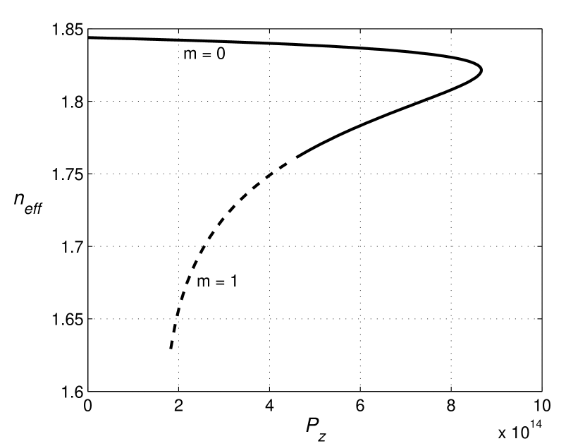
(a)

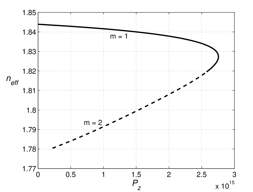
(b)

Figure 8: Dependence of the effective index $n_{eff}$ on power. Mode marks $m=0$ and $m=1$ are used in ($a$), $m=1$ and $m=2$ are used in ($b$).

There two curves corresponding to $\nu>0$ and $\nu<0$, which are convergent at value of $P_{z}$ corresponding to $A_{0}^{2}=2/\varepsilon_{K}(p/k_{0})^{2}$, Fig. 8. The curve with $\nu>0$ presents the dependence of the effective index on total power flux for a electric field varying with $x$ monotonically in the substrate.

As can be seen from Fig.8 at appropriate thickness of the waveguide and radiation frequency these modes can be excited independently of the power value. So, these guided wave modes are reduced to modes of the linear waveguide (13). To excite the modes of the $\nu<0$ branch the power must exceed some threshold value. For all branches the maximum of the power is limited.

The plots in Fig. 9) demonstrate the proportions of the power, which are localized in a substrate $P_{z}^{(1)}/P_{z}$, in a core $P_{z}^{(2)}/P_{z}$, and in a hyperbolic cover $P_{z}^{(3)}/P_{z}$ at $m=1$ and $m=2$ in case under consideration, $\varepsilon_{e}<\varepsilon_{2}$.

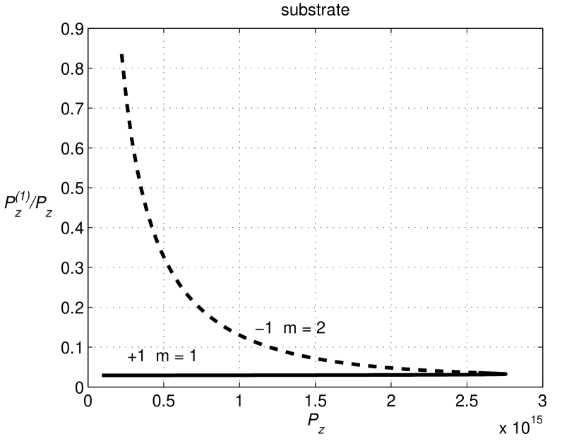
(a)

(c)

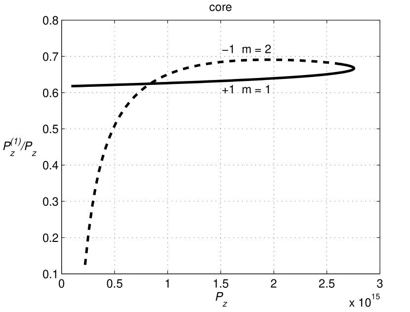
(b)

Figure 9: The power ration $P_{z}^{(1)}/P_{z}$ (a), $P_{z}^{(2)}/P_{z}$ (b) and $P_{z}^{(3)}/P_{z}$ as a function of $P_{z}$. Case $\varepsilon_{e}<\varepsilon_{2}$.

It follows that the radiation of mode with $\nu>0,m=1$ is localized principally in core and cover. This situation is little affected with increasing of the transferred power $P_{z}$. Oppositely, proportions of the power transported by mode with $\nu<0,m=2$ are changed over wide range under increasing of total transferred power. The principal part of the radiation is localized in the nonlinear substrate, but with increasing the $P_{z}$ the portion of radiation in the core grows. And The power in waveguide core for the modes of the $\nu<0$ branch can be greater then the transferred power by the modes of the $\nu>0$ branch.

For comparison purposes the same proportions are shown for the case $\varepsilon_{e}>\varepsilon_{2}$ in Fig. 9. It can be seen that the proportion of power in the covering layer is negligible in comparison with case $\varepsilon_{e}<\varepsilon_{2}$. It can be connected with the absence of the additional cut-off frequencies on the dielectric–hyperbolic material boundary.

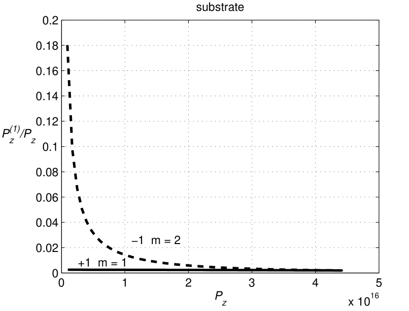
(a)

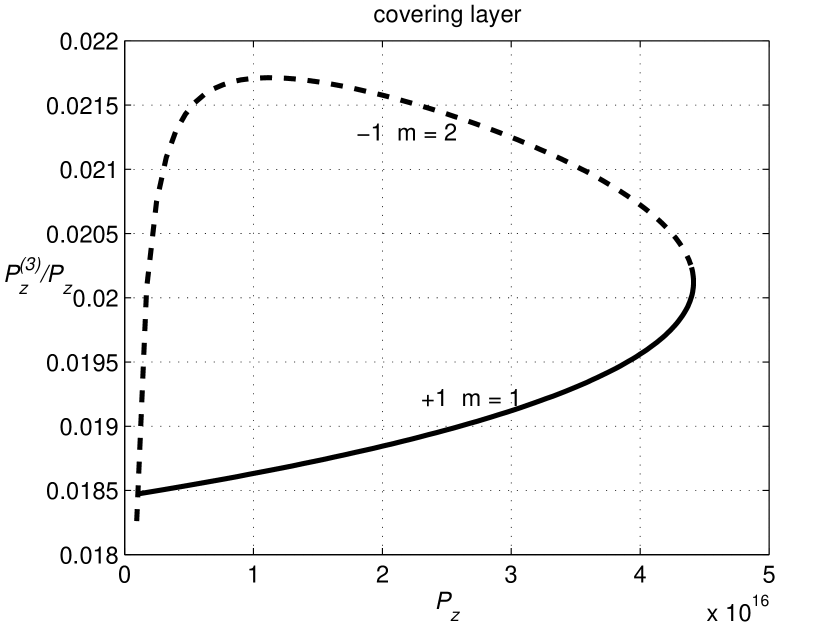
(c)

(b)

Figure 10: The power ration $P_{z}^{(1)}/P_{z}$ (a), $P_{z}^{(2)}/P_{z}$ (b) and $P_{z}^{(3)}/P_{z}$ as a function of $P_{z}$. Case $\varepsilon_{e}>\varepsilon_{2}$.

VI Conclusion

In the paper we have considered the TM-polarized linear and nonlinear guided waves which are guided by a linear dielectric slab embedded between linear or nonlinear substrate and uniaxial hyperbolic media. The anisotropy axis is aligned with a unit normal vector to the interface. In this geometry the TE wave is ordinary wave and the TM-polarized wave is the extra-ordinary one. The properties of the cover change the features of the guided TM waves. Both for a linear and for a nonlinear substrate the electromagnetic radiation can be confined in the waveguide under conditions $\varepsilon_{o}<0$, $\varepsilon_{e}>0$.

The electric and magnetic field transverse distributions and the dispersion relations are found in linear and nonlinear cases. In the linear case under condition that $\varepsilon_{e}<\varepsilon_{2}$ any guided wave mode has two cut-off frequencies. One of them corresponds to mode appearance, another corresponds to mode disappearance. It follows that there is a region of parameters in which the only several modes exist. It should be pointed that each conventional dielectric waveguide mode has only one cut-off frequency. It is worth noting that this phenomenon is unavailable in the case of a conventional waveguide. Usually the number of modes increases with core thickness or radiation frequency, and only single cut-off frequency exists. If $\varepsilon_{e}>\varepsilon_{2}$ then the single cut-off frequency exists for all modes marked $m\geq 1$. However, the fundamental mode with mark $m=0$ has the two cut-off frequencies. In the case of a conventional asymmetrical dielectric waveguide the single cut-off frequency is positive quantity. In the case under consideration one of the cut-off frequencies of the fundamental mode is to be negative quantity according to dispersion relation for the hyperbolic waveguide. It is imposable, thus the real magnitude of effective index is achieved at the zero film thickness and it is not equal zero. The property of the guided mode discussed above is the feature of hyperbolic asymmetrical slab waveguide.

In the nonlinear hyperbolic waveguide the modes can be collected in two sets. Both the dispersion curves and the modes (i.e., electric and magnetic field transverse distributions) are labeled by two numbers. One of them is $\pm 1$ in relation to the sign of the coordinate of the electric field strength maximum. If the maximum is localized in the nonlinear substrate then the coordinate $x_{0}<0$. If the maximum is localized outside substrate then the coordinate $x_{0}>0$, this is the case of virtual maximum. The second item of the label is integer $m$. It is the mode marker, which is present in the dispersion relations (16) and (31). The waveguide modes marked by $(+1,m)$ are reducible to the linear guiding modes. The modes with label $(-1,m)$ corresponds with situation where the peak of electric field is localized in the nonlinear substrate. These modes are absent in the linear waveguide. To excite these modes the power must exceed certain threshold value.

As the frequency of radiation or the film thickness changes, the dispersion curves marked $(+1,m)$ and dispersion curves marked $(-1,m+1)$ convergent in some point that is referred to as the transition point Lederer:85 . For the modes marked $m\geq 1$ these pictures in the case of hyperbolic and the conventional dielectric waveguide are similar in appearance. The exception is fundamental mode with $m=0$. The transition point is absent for this mode.

As in the case of linear case, the nonlinear hyperbolic waveguide under condition $\varepsilon_{e}<\varepsilon_{2}$ is characterized by the additional cut-off frequencies. Thus the number of modes is always limited.

Acknowledgments

We are grateful to Prof. I. Gabitov and Dr. C. Bayun for enlightening discussions. This investigation is funded by Russian Science Foundation (project 14-22-00098).

References

- (1) Noginov M. A., Barnakov Yu. A., Zhu G., Tumkur G., Li H., Narimanov E.E. Applied Physics Letters 94, 151105 (2009).
- (2) Xingjie Ni, Ishii Satoshi, Thoreson M.D., Shalaev Vl.M., Seunghoon Han, Sangyoon Lee, Kildishev Al.V. Optics Express 19 25242 (2011).
- (3) Drachev Vl.P., Podolskiy V.A., Kildishev A.V. Optics Express, 21 15048 (2013).
- (4) Shekhar P., Atkinson. J., Jacob Z. Nano Convergence, 1 1-17 (2014).
- (5) Wood B., Pendry J.B., Tsai D.P. Phys.Rev. B. 74, 115116 (2006).
- (6) Iorsh I.V. , Mukhin I.S. , Shadrivov I.V., Belov P.A., Kivshar Yu.S. Phys.Rev. B. 87, 075416 (2013) [6 pages].
- (7) Othman M.A.K., Guclu C., Capolino F. Optics Express 21, 7614 (2013).
- (8) Zapata-Rodriguez C.J., J. Miret J.J., Vukovic S., Belic M.R. Optics Express 21, 19113 (2013).
- (9) Jing Zhao, Hao Zhang, Xiangchao Zhang, Dahai Li, Hongliang Lu, Min Xu. Photon. Res. 1, 160 (2013).
- (10) Poddubny Al.N., Belov P.A., Ginzburg P., Zayats A.V., Kivshar Yu. S. Phys.Rev. B. 86, 035148 (2012).
- (11) Poddubny Al.N., Belov P.A., Kivshar Yu.S. Phys.Rev. A. 87, 035136 (2013).
- (12) Newman W.D., Cortes C.L., and Zubin J. J.Opt.Soc.Amer. B. 30, 766 (2013).
- (13) Ferrari L., Dylan Lu, Lepage D., Zhaowei Liu. Optics Express 22, 4301 (2014).
- (14) Benedicto J., Centeno E., Polles R., Moreau A. Phys.Rev. B. 88, 245138 (2013).
- (15) Ishii Satoshi, Shalaginov M.Y., Babicheva V.E., Boltasseva Al., Kildishev Al.V. Optics Letters 39, 4663 (2014).
- (16) Babicheva V.E., Shalaginov M.Y., Ishii Satoshi, Boltasseva A., Kildishev A.V. Optics Express 23, 9681 (2015).
- (17) Lyashko E.I., Maimistov A.I. Quantum Electronics 45 1050 (2015).
- (18) Hansperger R.G. Integrated Optics: Theory and Technology. (Berlin, Heidelberg, New York, Tokyo, Springer-Verlag, 1984)
- (19) Stegeman G.I., Seaton C.T. J.Appl.Phys. 58, R57-R78 (1985).
- (20) Mihalache D., Mazilu D. Solid State Commun. 60, 397-399 (1986)
- (21) Agranovich V.M. , Babichenko V.S. , Chernyak V.Ya. JETP Lett. 32, 512-515 (1980).
- (22) Lederer, F., Langbein U., and Ponath H.-E. Appl.Phys. B. 31, 187-190 (1983).
- (23) Langbein U., Lederer F., Ponath H.-E., and Trutschel U. Appl. Phys. B. 36, 187–193 (1985).
- (24) Kogelnik H. and Weber H.P. J.Opt.Soc.Amer. 64, 174–185 (1974).