Exact Post-Selection Inference for Changepoint Detection and Other Generalized Lasso Problems

Abstract

We study tools for inference conditioned on model selection events that are defined by the generalized lasso regularization path. The generalized lasso estimate is given by the solution of a penalized least squares regression problem, where the penalty is the $\ell_{1}$ norm of a matrix $D$ times the coefficient vector. The generalized lasso path collects these estimates as the penalty parameter $\lambda$ varies (from $\infty$ down to 0). Leveraging a (sequential) characterization of this path from Tibshirani & Taylor (2011), and recent advances in post-selection inference from Lee et al. (2016); Tibshirani et al. (2016), we develop exact hypothesis tests and confidence intervals for linear contrasts of the underlying mean vector, conditioned on any model selection event along the generalized lasso path (assuming Gaussian errors in the observations).

Our construction of inference tools holds for any penalty matrix $D$. By inspecting specific choices of $D$, we obtain post-selection tests and confidence intervals for specific cases of generalized lasso estimates, such as the fused lasso, trend filtering, and the graph fused lasso. In the fused lasso case, the underlying coordinates of the mean are assigned a linear ordering, and our framework allows us to test selectively chosen breakpoints or changepoints in these mean coordinates. This is an interesting and well-studied problem with broad applications; our framework applied to the trend filtering and graph fused lasso cases serves several applications as well. Aside from the development of selective inference tools, we describe several practical aspects of our methods such as (valid, i.e., fully-accounted-for) post-processing of generalized estimates before performing inference in order to improve power, and problem-specific visualization aids that may be given to the data analyst for he/she to choose linear contrasts to be tested. Many examples, both from simulated and real data sources, are presented to examine the empirical properties of our inference methods.

Keywords: generalized lasso, fused lasso, trend filtering, changepoint detection, post-selection inference

1 Introduction

Consider a classic Gaussian model for observations $y\in\mathbb{R}^{n}$, with known marginal variance $\sigma^{2}>0$,

$$y\sim\mathcal{N}(\theta,\sigma^{2}I),$$ (1)

where the (unknown) mean $\theta\in\mathbb{R}^{n}$ is the parameter of interest. In this paper, we examine problems in which $\theta$ is believed to have some specific structure (at least approximately so), in that it is sparse when parametrized with respect to a particular basis. A key example is the changepoint detection problem, in which the components of the mean $\theta_{1},\ldots,\theta_{n}$ correspond to ordered underlying positions (or locations) $1,\ldots,n$, and many adjacent components $\theta_{i}$ and $\theta_{i+1}$ are believed to be equal, with the exception of a sparse number of breakpoints or changepoints to be determined. See the left plot in Figure 1 for a simple example.

Many methods are available for estimation and detection in the changepoint problem. We focus on the 1-dimensional fused lasso (Tibshirani et al., 2005), also called 1-dimensional total variation denoising (Rudin et al., 1992) in signal processing, for reasons that will become clear shortly. This method, which we call the 1d fused lasso (or simply fused lasso) for short, is often used for piecewise constant estimation of the mean, but it does not come with associated inference tools after changepoints have been detected. In the top right panel of Figure 1, we inspect the 1d fused lasso estimate that has been tuned to detect two changepoints, in a data model where the mean $\theta$ only has one true changepoint. Writing the changepoint locations as $1\leq I_{1}<I_{2}\leq n$, we might consider testing

$$H_{0,j}:\theta_{I_{j-1}}=\ldots=\theta_{I_{j}-1}=\theta_{I_{j}}=\ldots=\theta_{I_{j+1}-1}\quad\text{versus}\\ H_{1,j}:\theta_{I_{j-1}}=\ldots=\theta_{I_{j}-1}\neq\theta_{I_{j}}=\ldots=\theta_{I_{j+1}-1},\quad j=1,2,$$

where we write $I_{0}=1$ and $I_{3}=n+1$ for notational convenience. If we were to naively ignore the data-dependent nature of $I_{1},I_{2}$ (these are the estimated changepoints from the two-step fused lasso procedure), i.e., treat them as fixed, then the natural tests for the null hypothesess $H_{0,j}$, $j=1,2$ would be to reject for large magnitudes of the statistics

$$T_{j}=\bar{y}_{(I_{j-1}):(I_{j}-1)}-\bar{y}_{(I_{j}):(I_{j+1}-1)},\quad j=1,2,$$

respectively, where we use $\bar{y}_{a:b}=\sum_{i=a}^{b}y_{i}/(b-a)$ to denote the average of components of $y$ between positions $a$ and $b$. Indeed, these can be seen as likelihood ratio tests stemming from the Gaussian model in (1).

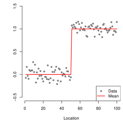
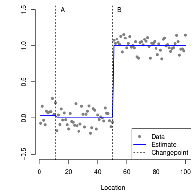
	Location	Naive p-values	TG p-values
A	11	0.057	0.359
B	50	0.000	0.000

Figure 1: A simple example with $n=100$ points generated around a piecewise constant mean with one true changepoint at location 50, shown in the top left panel. The 1d fused lasso path, stopped at the (end of the) second step, produces the estimate in the top right panel, with two detected changepoints at locations 11 and 50, labeled $A$ and $B$ in the figure. The table reports p-values from the naive Z-test, which does not account for the data-dependent nature of the changepoints, and from our TG test for the 1d fused lasso, which does.

The table in Figure 1 shows the results of running such naive Z-tests. At location $I_{2}$ (labeled location $B$ in the figure), which corresponds to a true changepoint in the underlying mean, the test returns a very small p-value, as expected. But at location $I_{1}$ (labeled $A$ in the figure), a spurious detected changepoint, the naive Z-test also produces a small p-value. This happens because the location $I_{1}$ has been selected by the 1d fused lasso, which inexorably links it to an unusually large magnitude of $T_{1}$; in other words, it is no longer appropriate to compare $T_{1}$ against its supposed Gaussian null distribution, with mean zero and variance $\sigma^{2}(1/(I_{1}-I_{0})+1/(I_{2}-I_{1}))$. Also shown in the table are the results of running our new truncated Gaussian (TG) test for the 1d fused lasso, which properly accounts for the data-dependent nature of the changepoints detected by fused lasso, and produces p-values that are exactly uniform under the null, conditional on $I_{1},I_{2}$ having been selected by the fused lasso in the first place. We now see that only the changepoint at location $I_{2}$ has a small associated p-value.

1.1 Summary

In this paper, we make the following contributions.

• We introduce the usage of post-selection inference tools to selection events defined by a class of methods called generalized lasso estimators. The key mathematical task is to show that the model selection event defined by any (fixed) step the generalized lasso solution path can be expressed as a polyhedron in the observation vector $y$ (Section 3.1). The (conditionally valid) TG tests and confidence intervals of Lee et al. (2016); Tibshirani et al. (2016) can then be applied, to test or cover any linear contrast of the mean vector $\theta$.

• We describe a stopping rule based on a generic information criterion (akin to AIC or BIC), to select a step along the generalized lasso path at which we are to perform conditional inference. We give a polyhedral representation for the ultimate model selection event that encapsulates both the selected path step and the generalized lasso solution at this step (Section 3.2). Along with the TG tests and confidence intervals, this makes for a practical (nearly-automatic) and broadly applicable set of inference tools.

• We study various special cases of the generalized lasso problem—namely, the 1d fused lasso, trend filtering, graph fused lasso, and regression problems—and for each, we develop specific forms for linear contrasts that can be used to test different population quantities of interest (Sections 4.1 through 4.5). In each case, we believe that our tests provide new advancements in the set of currently available inferential tools. For example, in the 1d fused lasso, i.e., the changepoint detection problem, our tests are the first that we know of that are specifically designed to yield proper inferences after changepoint locations have been detected.

• We present two of extensions of the basic tools described above for post-selection inference in generalized lasso problems: a post-processing tool, to improve the power of our methods, and a visualization aid, to improve practical useability.

• We conduct a comprehensive simulations across the various special problem cases, to investigate the (conditional) power of our methods, and verify their (conditional) type I error control (Sections 5.1 through 5.5). We also demonstrate a realistic application of our selective inference tools for changepoint detection to a data set of comparative genomic hybridization (CGH) measurements from two glioblas-toma multiforme (GBM) tumors (Section 5.6).

1.2 Related work

Post-selection inference, also known as selective inference, is a new but rapidly growing field. Unlike other recent developments in high-dimensional inference using a more classic full-population model, the point of selective inference is to provide a means of testing hypotheses derived from a selected model, the output of an algorithm that has been applied to data at hand. In a sequence of papers, Leeb & Potscher (2003, 2006, 2008) prove impossibility results about estimating the post-selection distribution of certain estimators in a classical regression setting. Berk et al. (2013), Lockhart et al. (2014) circumvent this by more directly conducting inference on post-selection targets (rather than basing inference on the distribution of the post-selection estimator itself). The former work is very broad and considers all selection mechanisms in regression (hence yielding more conservative inference); the latter is much more specific and considers the lasso estimator in particular. Lee et al. (2016); Tibshirani et al. (2016) improve on the method in Lockhart et al. (2014), and introduced a pivot-based framework for post-selection inference. Lee et al. (2016) describe the application to the lasso problem at a fixed tuning parameter $\lambda$; Tibshirani et al. (2016) describe the application to the lasso path at a fixed number of steps $k$ (and also, the least angle regression and forward stepwise paths). A number of extensions to different problem settings are given in Lee & Taylor (2014); Reid et al. (2014); Loftus & Taylor (2014); Choi et al. (2014). Asymptotics for non-Gaussian error distributions are presented in Tian & Taylor (2015a); Tibshirani et al. (2015). A broad treatment of selective inference in exponential family models and selective power is presented in Fithian et al. (2014). An improvement based on auxiliary randomization is considered in Tian & Taylor (2015b). A study of selective sequential tests and stopping rules is given in Fithian et al. (2015). Ours is the first work to consider selective inference in structural problems like the generalized lasso.

Changepoint detection carries a huge body of literature; reviews can be found in, e.g., Brodsky & Darkhovski (1993); Chen & Gupta (2000); Eckley et al. (2011). Far sparser is the literature on changepoint inference, say, inference for the location or size of changepoints, or segment lengths. Hinkley (1970); Worsley (1986); Bai (1999) are some examples, and Jandhyala et al. (2013); Horvath & Rice (2014) provide nice surveys and extensions. The main tools are built around likelihood ratio test statistics comparing two nested changepoint models, but at fixed locations. Since interesting locations to be tested are typically estimated, these inferences can be clearly invalid (if estimation and inference are both done on the same data samples).

Probably most relevant to our goal of valid post-selection changepoint inference is Frick et al. (2014), who develop a simultaneous confidence band for the mean in a changepoint model. Their Simultaneous Multiscale Changepoint Estimator (SMUCE) seeks the most parsimonious piecewise constant fit subject to an upper limit on a certain multiscale statisic, and is solved via dynamic programming. Because the final confidence band has simultaneous coverage (over all components of the mean), it also has valid coverage for any (data-dependent) post-selection target. In contrast, our proposal does not give simultaneous coverage of the mean, but rather, selective coverage of a particular post-selection target. An empirical comparison between the two methods (SMUCE, and ours) is given in Section 5.2. While this comparison is useful and informative, it is also worth emphasizing that the framework in this paper applies far outside of the changepoint detection problem, i.e., to trend filtering, graph clustering, and regression problems with structured coefficients.

1.3 Notation

For a matrix $D$, we will denote by $D_{S}$ the submatrix whose rows are in a set $S\subseteq\{1,\ldots,m\}$. We write $D_{-S}$ to mean $D_{S^{c}}=D_{\{1,\ldots,m\}\setminus S}$. Similarly, for a vector $x$, we write $x_{S}$ or $x_{-S}$ to extract the subvector whose components are in $S$ or not in $S$, respectively. We use $A^{+}$ for the pseudoinverse of a matrix $A$, and $\mathrm{row}(A)$, $\mathrm{col}(A)$, $\mathrm{null}(A)$ for the column space, row space, and null space of $A$, respectively. We write $P_{L}$ for the projection matrix onto a linear subspace $L$. Lastly, we will often abbreviate a sequence $(x_{1},\ldots,x_{k})$ by $x_{1:k}$.

2 Preliminaries

2.1 The generalized lasso regularization path

Given a response $y\in\mathbb{R}^{n}$, the generalized lasso estimator is defined by the optimization problem

$$\hat{\beta}=\mathop{\mathrm{argmin}}_{\beta\in\mathbb{R}^{n}}\;\frac{1}{2}\|y-X\beta\|_{2}^{2}+\lambda\|D\beta\|_{1},$$ (2)

where $X\in\mathbb{R}^{n\times p}$ is a matrix of predictors, $D\in\mathbb{R}^{m\times p}$ is a prespecified penalty matrix, and $\lambda\geq 0$ is a regularization parameter. This matrix $D$ is chosen so that sparsity of $D\hat{\beta}$ induces some type of desired structure in the solution $\hat{\beta}$ in (2). Important special cases, each corresponding to a specific class of matrices $D$, include the 1d fused lasso, trend filtering, and graph fused lasso problems. More details on these problems is given in Section 4; see also Section 2 in Tibshirani & Taylor (2011).

We review the algorithm of Tibshirani & Taylor (2011) to compute the entire solution path in (2), i.e., the continuum of solutions $\hat{\beta}(\lambda)$ as the regularization parameter $\lambda$ desends from $\infty$ to 0. We focus on the problem of signal approximation, where $X=I$:

$$\hat{\beta}=\mathop{\mathrm{argmin}}_{\beta\in\mathbb{R}^{n}}\;\frac{1}{2}\|y-\beta\|_{2}^{2}+\lambda\|D\beta\|_{1}.$$ (3)

For a general $X$, a simple modification to the arguments used for (3) will deliver the solution path for (2), and we refrain from describing this until Section 4.5. The path algorithm of Tibshirani & Taylor (2011) for (3) is derived from the perspective of its equivalent Lagrange dual problem, namely

$$\hat{u}=\mathop{\mathrm{argmin}}_{u\in\mathbb{R}^{m}}\;\|y-D^{T}u\|_{2}^{2}\;\;\mathop{\mathrm{subject\,\,to}}\;\;\|u\|_{\infty}\leq\lambda.$$ (4)

The primal and dual solutions, $\hat{\beta}$ in (3) and $\hat{u}$ in (4), are related by

$$\hat{\beta}=y-D^{T}\hat{u},$$ (5)

as well as

$$\hat{u}_{i}\in\begin{cases}\{+1\}&\text{if $(D\hat{\beta})_{i}>0$}\\ \{-1\}&\text{if $(D\hat{\beta})_{i}<0$}\\ [-1,1]&\text{if $(D\hat{\beta})_{i}=0$}\end{cases},\quad i=1,\ldots,m.$$ (6)

The strategy is now to compute a solution path $\hat{u}(\lambda)$ in the dual problem, as $\lambda$ descends from $\infty$ to 0, and then use (5) to deliver the primal solution path. Therefore it suffices to describe the path algorithm as it operates on the dual problem; this is given next.

Algorithm 1 (Dual path algorithm for the generalized lasso, $X=I$).

Given $y\in\mathbb{R}^{n}$ and $D\in\mathbb{R}^{m\times n}$.

1. Compute $\hat{u}=(DD^{T})^{+}Dy$, and compute the first hitting time,

   $$\lambda_{1}=\max_{i=1,\ldots,m}\;|\hat{u}_{i}|.$$

   Define the hitting coordinate $i_{1}$ to be the argmax of the above expression, and define the hitting sign $r_{1}=\mathrm{sign}(\hat{u}_{i_{1}})$. Initialize the boundary set $\mathcal{B}_{1}=\{i_{1}\}$ and the boundary sign list $s_{\mathcal{B}_{1}}=(r_{1})$. Record the solution as $\hat{u}(\lambda)=\hat{u}$ over $\lambda\in[\lambda_{1},\infty)$, and set $k=1$.

2. While $\lambda_{k}>0$:

   1. Compute $a=(D_{-\mathcal{B}_{k}}D_{-\mathcal{B}_{k}}^{T})^{+}D_{-\mathcal{B}_{k}}y$ and $b=(D_{-\mathcal{B}_{k}}D_{-\mathcal{B}_{k}}^{T})^{+}D_{-\mathcal{B}_{k}}D_{\mathcal{B}_{k}}^{T}s_{\mathcal{B}_{k}}$. Also define

      $$c =\mathrm{diag}\big{(}s_{\mathcal{B}_{k}}\big{)}D_{\mathcal{B}_{k}}(y-D_{-\mathcal{B}_{k}}^{T}a),$$

      $$d =\mathrm{diag}\big{(}s_{\mathcal{B}_{k}}\big{)}D_{\mathcal{B}_{k}}(D_{\mathcal{B}_{k}}^{T}s-D_{-\mathcal{B}_{k}}^{T}b).$$

   2. Compute the next hitting time,

      $$\lambda_{k+1}^{\mathrm{hit}}=\max_{i\notin\mathcal{B}_{k},\;r\in\{-1,1\}}\;\frac{a_{i}}{r+b_{i}}\cdot\mathds{1}\Bigg{\{}\frac{a_{i}}{r+b_{i}}\geq 0\Bigg{\}}.$$ (7)

      Define the hitting coordinate $i^{\mathrm{hit}}_{k+1}$ and hitting sign $r^{\mathrm{hit}}_{k+1}$ to be the pair achieving the maximum in the above expression.

   3. Compute the next leaving time,

      $$\lambda_{k+1}^{(\mathrm{leave})}=\mathop{\mathrm{argmax}}_{i\in\mathcal{B}_{k}}\;\frac{c_{i}}{d_{i}}\cdot\mathds{1}\Big{\{}c_{i}\leq 0,\;d_{i}<0\Big{\}},$$ (8)

      Define the leaving coordinate $i^{\mathrm{leave}}_{k+1}$ to be the argmax of the above expression, and define the leaving sign $r^{\mathrm{leave}}_{k+1}=r_{i^{\mathrm{leave}}_{k+1}}$.

   4. Define the next knot according to

      $$\lambda_{k+1}=\max\Big{\{}\lambda_{k+1}^{(\mathrm{hit})},\;\lambda_{k+1}^{(\mathrm{leave})}\Big{\}}.$$ (9)

      If the next hitting time is larger, $\lambda_{k+1}^{(\mathrm{hit})}\geq\lambda_{k+1}^{(\mathrm{leave})}$, then define the new boundary set $\mathcal{B}_{k+1}$ by appending the hitting coordinate $i^{\mathrm{hit}}_{k+1}$ to $\mathcal{B}_{k}$, and define the new boundary sign list $s_{\mathcal{B}_{k+1}}$ by appending the hitting sign $r^{\mathrm{hit}}_{k+1}$ to $s_{\mathcal{B}_{k}}$. Otherwise, define $\mathcal{B}_{k+1}$ by removing the leaving coordinate from $i^{\mathrm{leave}}_{k+1}$ from $\mathcal{B}_{k}$ and define $s_{\mathcal{B}_{k+1}}$ by removing the leaving sign $r^{\mathrm{leave}}_{k+1}$ from $s_{\mathcal{B}_{k}}$. Record the solution as $\hat{u}(\lambda)=a-\lambda b$ over $\lambda\in[\lambda_{k+1},\lambda_{k}]$, and update $k=k+1$.

Explained in words, the dual path algorithm in Algorithm 1 tracks the coordinates of the computed dual solution $\hat{u}(\lambda)$ that are equal to $\pm\lambda$, i.e., that lie on the boundary of the constraint region $[-\lambda,\lambda]^{m}$. The collection of such coordinates, at any given step $k$ in the path, is called the boundary set, and is denoted $\mathcal{B}_{k}$. Critical values of the regularization parameter at which the boundary set changes (i.e., at which coordinates join or leave the boundary set) are called knots, and are denoted $\lambda_{1}\geq\lambda_{2}\geq\ldots\geq 0$. From the form of the dual solution $\hat{u}(\lambda)$ as presented in Algorithm 1, and the primal-dual relationship (5), the primal solution path may be expressed in terms of the current boundary set $\mathcal{B}_{k}$ and boundary sign list $s_{\mathcal{B}_{k}}$, as in

$$\hat{\beta}(\lambda)=P_{\mathrm{null}(D_{-\mathcal{B}_{k}})}(y-\lambda D_{\mathcal{B}_{k}}^{T}s_{\mathcal{B}_{k}})\quad\text{for $\lambda\in[\lambda_{k+1},\lambda_{k}]$},$$ (10)

As we can see, the primal solution lies in the subspace $\mathrm{null}(D_{-\mathcal{B}_{k}})$, which implies it expresses a certain type of structure. This will become more concrete as we look at specific cases for $D$ in Section 4, but for now, the important point is that the structure of the generalized lasso solution (10) is determined by the boundary set $\mathcal{B}_{k}$. Therefore, by conditioning on the observed boundary set $\mathcal{B}_{k}$ after a certain number of steps $k$ of the path algorithm, we are effectively conditioning of the observed model structure in the generalized lasso solution at this step. This is essentially what is done in Section 3.

Lastly, we note the following important point. In some generalized lasso problems, Step 2(c) in Algorithm 1 does not need to be performed, i.e., we can formally replace this step by $\lambda_{k+1}^{\mathrm{leave}}=0$, and accordingly, the boundary set $\mathcal{B}_{k}$ will only grow over iterations $k$. This is true, e.g., for all 1d fused lasso problems; more generally, it is true for any generalized lasso signal approximator problem in which $DD^{T}$ is diagonally dominant.

2.2 Exact inference after polyhedral conditioning

Under the Gaussian observation model in (1), Lee et al. (2016); Tibshirani et al. (2016) build a framework for inference on an arbitrary linear constrast $v^{T}\theta$ of the mean $\theta$, conditional on $y\in G$, where $G\subseteq\mathbb{R}^{n}$ is an arbitrary polyhedron. A core tool in these works is an exact pivotal statistic for $v^{T}\theta$, conditional on $y\in G$: they prove that there exists random variables $\mathcal{V}^{\mathrm{lo}},\mathcal{V}^{\mathrm{up}}$ such that

$$F^{[\mathcal{V}^{\mathrm{lo}},\mathcal{V}^{\mathrm{up}}]}_{v^{T}\theta,\sigma^{2}\|v\|_{2}^{2}}(v^{T}y)\;\Big{|}\;y\in G\;\sim\mathrm{Unif}[0,1],$$ (11)

where $F^{[a,b]}_{\mu,\tau^{2}}$ denotes the cumulative distribution function of a univariate Gaussian random variable $Z\sim\mathcal{N}(\mu,\tau^{2})$ conditional on lying in the interval $[a,b]$. The above is called the truncated Gaussian (TG) pivot. The truncation limits $\mathcal{V}^{\mathrm{lo}},\mathcal{V}^{\mathrm{up}}$ are easily computable, given a half-space representation for the polyhedron $G=\{x:\Gamma x\geq w\}$, where $\Gamma\in\mathbb{R}^{q\times n}$ and $w\in\mathbb{R}^{n}$ and the inequality here is to be interpreted componentwise. Specifically, we have

$$\mathcal{V}^{\mathrm{lo}}(y) =v^{T}y-\min_{j:\rho_{j}>0}\frac{(\Gamma y)_{j}-w_{j}}{\rho_{j}},$$

$$\mathcal{V}^{\mathrm{up}}(y) =v^{T}y-\max_{j:\rho_{j}<0}\frac{(\Gamma y)_{j}-w_{j}}{\rho_{j}},$$

where $\rho=\Gamma v/\|v\|^{2}$. The TG pivotal statistic in (11) enables us to test the null hypothesis $H_{0}:v^{T}\theta=0$ against the one-sided alternative $H_{1}:v^{T}\theta>0$. Namely, it is clear that the TG test statistic

$$T=1-F^{[\mathcal{V}^{\mathrm{lo}},\mathcal{V}^{\mathrm{up}}]}_{0,\sigma^{2}\|v\|_{2}^{2}}(v^{T}y)$$ (12)

is itself a p-value for $H_{0}$, with finite sample validity, conditional on $y\in G$. (A two-sided test is also possible: we simply use $2\min\{T,1-T\}$ as our p-value; see Tibshirani et al. (2016) for a discussion of the merits of one-sided and two-sided selective tests.) Confidence intervals follow directly from (11) as well. For an (equi-tailed) interval with exact finite sample coverage $1-\alpha$, conditional on the event $y\in G$, we take $[\delta_{\alpha/2},\delta_{1-\alpha/2}]$, where $\delta_{\alpha/2},\delta_{1-\alpha/2}$ are obtained by inverting the TG pivot, i.e., defined to satisfy

$$1-F^{[\mathcal{V}^{\mathrm{lo}},\mathcal{V}^{\mathrm{up}}]}_{\delta_{\alpha/2},\sigma^{2}\|v\|_{2}^{2}}(v^{T}y) =\alpha/2,$$ (13)

$$1-F^{[\mathcal{V}^{\mathrm{lo}},\mathcal{V}^{\mathrm{up}}]}_{\delta_{1-\alpha/2},\sigma^{2}\|v\|_{2}^{2}}(v^{T}y) =1-\alpha/2.$$

At this point, it may seem unclear how this framework applies to post-selection inference in generalized lasso problems. The key ingredients are, of course, the polyhedron $G$ and the contrast vector $v$. In the next section, we will show how to construct polyhedra that correspond to model selection events of interest, at points along the generalized lasso path. In the following section, we will suggest choices of contrast vectors that lead to interesting and useful tests in specific settings, such as the 1d fused lasso, trend filtering, and graph fused lasso problems.

2.3 Can we not just use lasso inference tools?

When the penalty matrix $D$ is square and invertible, the generalized lasso problem (2) is equivalent to a lasso problem, in the variable $\alpha=D\beta$, with design matrix $XD^{-1}$. More generally, when $D$ has full row rank, problem (2) is reducible to a lasso problem (see Tibshirani & Taylor (2011)). In this case, existing inference theory for the lasso path (from Tibshirani et al. (2016)) could be applied to the equivalent lasso problem, to perform post-selection inference on generalized lasso models. This covers inference for the 1d fused lasso and trend filtering problems. But when $D$ is row rank deficient (when it has more rows than columns), the generalized lasso is not equivalent to a lasso problem (see again Tibshirani & Taylor (2011)), and we cannot simply resort to lasso inference tools. This would hence rule out treating problems like the 2d fused lasso, the graph fused lasso (for any graph with more edges than nodes), the sparse 1d fused lasso, and sparse trend filtering from a pure lasso perspective. Our paper presents a unified treatment of post-selection inference across all generalized lasso problems, regardless of the penalty matrix $D$.

3 Inference along the generalized lasso path

3.1 The selection event after a given number of steps $k$

Here, we suppose that we have run a given (fixed) number of steps $k$ of the generalized lasso path algorithm, and we have a contrast vector $v$ in mind, such that $v^{T}\theta$ is a parameter of interest (to be tested or covered). Define the generalized lasso model at step $\ell$ of the path to be

$$M_{\ell}=(\mathcal{B}_{\ell},s_{\mathcal{B}_{\ell}},R^{\mathrm{hit}}_{\ell},I^{\mathrm{leave}}_{\ell}),$$

where $\mathcal{B}_{\ell},s_{\mathcal{B}_{\ell}}$ are the boundary set and signs at step $\ell$, and $R^{\mathrm{hit}}_{\ell},I^{\mathrm{leave}}_{\ell}$ are quantities to be defined shortly. We will show that the entire model sequence from steps $\ell=1,\ldots,k$, denoted $M_{1:k}=(M_{1},\ldots,M_{k})$, is a polyhedral set in $y$. By this we mean the following: if $\widehat{M}_{1:k}(y)$ denotes the model sequence as a function of $y$, and $M_{1:k}$ a given realization, then the set

$$G_{k}=\{y:\widehat{M}_{1:k}(y)=M_{1:k}\}$$

is a polyhedron, more specifically, a convex cone, and can therefore be expressed as $G_{k}=\{y:\Gamma y\geq 0\}$ for a matrix $\Gamma=\Gamma(M_{1:k})$ that we will show how to construct, based on $M_{1:k}$.

Our construction uses induction. When $k=1$, and we write $\mathcal{B}_{1}=\{i_{1}\}$ and $s_{\mathcal{B}_{1}}=(r_{1})$, it is clear from the first step of Algorithm 1 that $(i_{1},r_{1})$ is the hitting coordinate-sign pair if and only if

$$r_{1}[(DD^{T})^{+}D]_{i_{1}}\,y \geq[(DD^{T})^{+}D]_{i}\,y,\quad i\neq i_{1},$$

$$r_{1}[(DD^{T})^{+}D]_{i_{1}}\,y \geq-[(DD^{T})^{+}D]_{i}\,y,\quad i\neq i_{1}.$$

Hence we can construct $\Gamma(M_{1})$ to have the corresponding $2(m-1)$ rows—to be explicit, these are $r_{1}[(DD^{T})^{+}D]_{i_{1}}\pm[(DD^{T})^{+}D]_{i}$, $i\neq i_{1}$. We note that at the first step, there is no characterization needed for $R^{\mathrm{hit}}_{1}$ and $I^{\mathrm{leave}}_{1}$ (for simplicity, we may think of these as being empty sets).

Now assume that, given a model sequence $M_{1:(k+1)}=(M_{1},\ldots,M_{k+1})$, we have constructed a polyhedral representation for $G_{k}=\{y:\widehat{M}_{1:k}(y)=M_{1:k}\}$, i.e., we have constructed a matrix $\Gamma(M_{1:k})$ such that $G_{k}=\{y:\Gamma(M_{1:k})\geq 0\}$. To show that $G_{k+1}=\{y:\Gamma(M_{1:(k+1)})\geq 0\}$ can also be written in the analogous form, we will define $\Gamma(M_{1:{k+1}})$ by appending rows to $\Gamma(M_{1:k})$ that capture the generalized lasso model at step $k+1$ of Algorithm 1. We will add rows to characterize the hitting time (7), leaving time (8), and the next action (either hitting or leaving) (9). Keeping with the notation in (7), a simple argument shows that the next hitting time can be alternatively written as

$$\lambda_{k+1}^{\mathrm{hit}}=\max_{i\notin\mathcal{B}_{k}}\;\frac{a_{i}}{\mathrm{sign}(a_{i})+b_{i}}.$$

Plugging in for $a,b$, we may characterize the viable hitting signs at step $k+1$, $R^{\mathrm{hit}}_{k+1}=\{r_{k,i}:i\notin\mathcal{B}_{k}\}$, as well as the next hitting coordinate and hitting sign, $i^{\mathrm{hit}}_{k+1}$ and $r^{\mathrm{hit}}_{k+1}$, by the following inequalities:

$$r_{k,i}\,[(D_{-\mathcal{B}_{k}}D_{-\mathcal{B}_{k}}^{T})^{+}D_{-\mathcal{B}_{k}}]_{i}\,y \geq 0,\quad i\notin\mathcal{B}_{k},$$

$$\frac{[(D_{-\mathcal{B}_{k}}D_{-\mathcal{B}_{k}}^{T})^{+}D_{-\mathcal{B}_{k}}]_{i^{\mathrm{hit}}_{k+1}}\,y}{r_{k}^{\mathrm{hit}}+[(D_{-\mathcal{B}_{k}}D_{-\mathcal{B}_{k}}^{T})^{+}D_{-\mathcal{B}_{k}}]_{i^{\mathrm{hit}}_{k+1}}\,D_{\mathcal{B}_{k}}^{T}s_{\mathcal{B}_{k}}} \geq\frac{[(D_{-\mathcal{B}_{k}}D_{-\mathcal{B}_{k}}^{T})^{+}D_{-\mathcal{B}_{k}}]_{i}\,y}{r_{k,i}+[(D_{-\mathcal{B}_{k}}D_{-\mathcal{B}_{k}}^{T})^{+}D_{-\mathcal{B}_{k}}]_{i}\,D_{\mathcal{B}_{k}}^{T}s_{\mathcal{B}_{k}}},\quad i\notin\mathcal{B}_{k}.$$

This corresponds to $2(m-|\mathcal{B}_{k}|)$ rows to be appended to $\Gamma(M_{1:k})$.

For (8), we first define the viable leaving coordinates, denoted $I^{\mathrm{leave}}_{k+1}$, by the subset of $i\in\mathcal{B}_{k}$ for which $c_{i}<0$ and $d_{i}<0$. We may write $I^{\mathrm{leave}}_{k+1}=C^{\mathrm{leave}}_{k+1}\cap D^{\mathrm{leave}}_{k+1}$, where $C^{\mathrm{leave}}_{k+1}$ is the set of $i$ for which $c_{i}<0$, and $D^{\mathrm{leave}}_{k+1}$ is the set of $i$ for which $d_{i}<0$. Plugging in for $c,d$, we notice that only the former set $C^{\mathrm{leave}}_{k+1}$ depends on $y$, and $D^{\mathrm{leave}}_{k+1}$ is deterministic once we have characterized $M_{1:k}$. This gives rise to the following inequalities determining $I^{\mathrm{leave}}_{k+1}=C^{\mathrm{leave}}_{k+1}\cap D^{\mathrm{leave}}_{k+1}$:

$$\big{[}\mathrm{diag}\big{(}s_{\mathcal{B}_{k}}\big{)}D_{\mathcal{B}_{k}}\big{(}I-D_{-\mathcal{B}_{k}}^{T}(D_{-\mathcal{B}_{k}}D_{-\mathcal{B}_{k}}^{T})^{+}D_{-\mathcal{B}_{k}}\big{)}\big{]}_{i}\,y \leq 0,\quad i\in C^{\mathrm{leave}}_{k+1}\cap D^{\mathrm{leave}}_{k+1},$$

$$\big{[}\mathrm{diag}\big{(}s_{\mathcal{B}_{k}}\big{)}D_{\mathcal{B}_{k}}\big{(}I-D_{-\mathcal{B}_{k}}^{T}(D_{-\mathcal{B}_{k}}D_{-\mathcal{B}_{k}}^{T})^{+}D_{-\mathcal{B}_{k}}\big{)}\big{]}_{i}\,y \geq 0,\quad i\in\big{(}C^{\mathrm{leave}}_{k+1}\big{)}^{c}\cap D^{\mathrm{leave}}_{k+1},$$

which corresponds to $|D^{\mathrm{leave}}_{k+1}|\leq|\mathcal{B}_{k}|$ rows to be appended to $\Gamma(M_{1:k})$. Given this characterization for $I^{\mathrm{leave}}_{k+1}$, we may now characterize the next leaving coordinate $i^{\mathrm{leave}}_{k+1}$ by:

$$\frac{\big{[}\mathrm{diag}\big{(}s_{\mathcal{B}_{k}}\big{)}D_{\mathcal{B}_{k}}\big{(}I-D_{-\mathcal{B}_{k}}^{T}(D_{-\mathcal{B}_{k}}D_{-\mathcal{B}_{k}}^{T})^{+}D_{-\mathcal{B}_{k}}\big{)}\big{]}_{i^{\mathrm{leave}}_{k+1}}\,y}{\big{[}\mathrm{diag}\big{(}s_{\mathcal{B}_{k}}\big{)}D_{\mathcal{B}_{k}}\big{(}I-D_{-\mathcal{B}_{k}}^{T}(D_{-\mathcal{B}_{k}}D_{-\mathcal{B}_{k}}^{T})^{+}D_{-\mathcal{B}_{k}}\big{)}\big{]}_{i^{\mathrm{leave}}_{k+1}}\,D_{\mathcal{B}_{k}}^{T}s_{\mathcal{B}_{k}}}\geq\\ \frac{\big{[}\mathrm{diag}\big{(}s_{\mathcal{B}_{k}}\big{)}D_{\mathcal{B}_{k}}\big{(}I-D_{-\mathcal{B}_{k}}^{T}(D_{-\mathcal{B}_{k}}D_{-\mathcal{B}_{k}}^{T})^{+}D_{-\mathcal{B}_{k}}\big{)}\big{]}_{i}\,y}{\big{[}\mathrm{diag}\big{(}s_{\mathcal{B}_{k}}\big{)}D_{\mathcal{B}_{k}}\big{(}I-D_{-\mathcal{B}_{k}}^{T}(D_{-\mathcal{B}_{k}}D_{-\mathcal{B}_{k}}^{T})^{+}D_{-\mathcal{B}_{k}}\big{)}\big{]}_{i}\,D_{\mathcal{B}_{k}}^{T}s_{\mathcal{B}_{k}}},\quad i\in I^{\mathrm{leave}}_{k+1}.$$

This corresponds to $|I^{\mathrm{leave}}_{k+1}|\leq|\mathcal{B}_{k}|$ rows that must be appended to $\Gamma(M_{1:k})$. Recall that the leaving coordinate is given by $r^{\mathrm{leave}}_{k+1}=r_{i^{\mathrm{leave}}_{k+1}}$.

Lastly, for (9), we either use

$$\frac{[(D_{-\mathcal{B}_{k}}D_{-\mathcal{B}_{k}}^{T})^{+}D_{-\mathcal{B}_{k}}]_{i^{\mathrm{hit}}_{k+1}}\,y}{r_{k}^{\mathrm{hit}}+[(D_{-\mathcal{B}_{k}}D_{-\mathcal{B}_{k}}^{T})^{+}D_{-\mathcal{B}_{k}}]_{i^{\mathrm{hit}}_{k+1}}\,D_{\mathcal{B}_{k}}^{T}s_{\mathcal{B}_{k}}}\geq\\ \frac{\big{[}\mathrm{diag}\big{(}s_{\mathcal{B}_{k}}\big{)}D_{\mathcal{B}_{k}}\big{(}I-D_{-\mathcal{B}_{k}}^{T}(D_{-\mathcal{B}_{k}}D_{-\mathcal{B}_{k}}^{T})^{+}D_{-\mathcal{B}_{k}}\big{)}\big{]}_{i^{\mathrm{leave}}_{k+1}}\,y}{\big{[}\mathrm{diag}\big{(}s_{\mathcal{B}_{k}}\big{)}D_{\mathcal{B}_{k}}\big{(}I-D_{-\mathcal{B}_{k}}^{T}(D_{-\mathcal{B}_{k}}D_{-\mathcal{B}_{k}}^{T})^{+}D_{-\mathcal{B}_{k}}\big{)}\big{]}_{i^{\mathrm{leave}}_{k+1}}\,D_{\mathcal{B}_{k}}^{T}s_{\mathcal{B}_{k}}}$$

if $\lambda^{\mathrm{hit}}_{k+1}\geq\lambda^{\mathrm{leave}}_{k+1}$, or the above with the inequality sign flipped, if $\lambda^{\mathrm{hit}}_{k+1}<\lambda^{\mathrm{leave}}_{k+1}$. In either case, only one more row is to be appended to $\Gamma(M_{1:k})$. This completes the inductive proof.

It is worth noting that, in the inductive step that constructs $\Gamma(M_{1:(k+1)})$ by appending rows to $\Gamma(M_{1:k})$, we append a total of at most $2(m-|\mathcal{B}_{k}|)+2|\mathcal{B}_{k}|+1=2m+1$ rows. Therefore after $k+1$ steps, the polyhedral representation for the model sequence $M_{1:(k+1)}$ uses a matrix $\Gamma(M_{1:(k+1)})$ with at most $(2m+1)(k+1)$ rows.

Combining the results of this subsection with the TG pivotal statistic from Section 2.2, we are now equipped to perform conditional inference on the model that is selected at any fixed step $k$ of the generalized lasso path. (Recall, we are assuming that a reasonable contrast vector $v$ has been determined such that $v^{T}\theta$ is a quantity of interest in the $k$-step generalized lasso model; in-depth discussion of reasonable choices of contrast vectors, for particular problems, is given in Section 4.) Of course, the choice of which step $k$ to analyze is somewhat critical. The high-level idea is to fix a step $k$ that is large enough for the selected model to be interesting, but not so large that our tests will be low-powered. In some practical applications, choosing $k$ a priori may be natural; e.g., in the 1d fused lasso problem, where the selected model correponds to detected changepoints (as discussed in the introduction), we may choose (say) $k=10$ steps, if in our particular setting we are interested in detecting and performing inference on at most 10 changepoints. But in most practical applications, fixing a step $k$ a priori is likely a difficult task. Hence, we present a rigorous strategy that allows the choice of $k$ to be data-driven, next.

3.2 The selection event after an IC-selected number of steps $k$

We develop approaches based on a generic information criterion (IC), like AIC or BIC, for selecting a number of steps $k$ along the generalized path that admits a “reasonable” model. By “reasonable”, our IC approach admits a $k$-step generalized lasso solution balances training error and some notion of complexity. Importantly, we specifically design our IC-based approaches so that the selection event determining $k$ is itself a polyhedral function of $y$. We establish this below.

Defined in terms of a generalized lasso model $M_{k}=(\mathcal{B}_{k},s_{\mathcal{B}_{k}},R^{\mathrm{hit}}_{k},I^{\mathrm{leave}}_{k})$ at step $k$, we consider the general form IC:

$$J(M_{k})=\|y-P_{\mathrm{null}(D_{-\mathcal{B}_{k}})}y\|_{2}^{2}+P_{n}\big{(}\mathrm{nullity}(D_{-\mathcal{B}_{k}})\big{)}.$$ (14)

The first term above is the squared loss between $y$ and its projection onto the subspace $\mathrm{null}(D_{-\mathcal{B}_{k}})$; recall that the $k$-step generalized lasso solution itself lies in this subspace, as written in (10), and so here we have replaced the squared loss between $y$ and $\hat{\beta}(\lambda_{k})$ with the squared error loss between $y$ and the unshrunken estimate $P_{\mathrm{null}(D_{-\mathcal{B}_{k}})}y$. (This is needed in order for our eventual IC-based rule to be equivalent to a polyhedral constraint in $y$, as will be seen shortly.) The second term in (14) utilizes $\mathrm{nullity}(D_{-\mathcal{B}_{k}})$, the dimension of $\mathrm{null}(D_{-\mathcal{B}_{k}})$, i.e., the dimension of the solution subspace. It hence penalizes the complexity associated with the $k$-step generalized lasso solution. Indeed, from Tibshirani & Taylor (2011, 2012), the quantity $\mathrm{nullity}(D_{-\mathcal{B}_{k}})$ is an unbiased estimate of the degrees of freedom of $\hat{\beta}(\lambda_{k})$. Further, $P_{n}$ is a penalty function that is allowed to depend on $n$ and $\sigma^{2}$ (the marginal variance in the observation model (1)). Some common choices are: $P_{n}(d)=2\sigma^{2}d$, which makes (14) like AIC; $P_{n}(d)=\sigma^{2}d\log{n}$, motivated by BIC; and $P_{n}(d)=\sigma^{2}(d\log{n}+2\gamma\log{n\choose d})$, where $\gamma\in(0,1)$ is a parameter to be chosen (say, $\gamma=1/2$ for simplicity), motivated by extended BIC (EBIC) of Chen & Chen (2008). Beyond these, any choice of complexity penalty will do as long as $P_{n}(d)$ is an increasing function of $d$.

Unfortunately, choosing to stop the path at the step that minimizes the IC defined in (14) does not define a polyhedron in $y$. Therefore, we use a modified IC-based rule. We first define

$$\widehat{I}^{\mathrm{IC}}(y)=\{1\}\cup\Big{\{}k\in\{2,3,\ldots\}:\mathrm{null}(D_{-\mathcal{B}_{k}})\neq\mathrm{null}(D_{-\mathcal{B}_{k-1}})\Big{\}},$$ (15)

the set of steps at which we see action (nonzero adjacent differences) in the IC. For $k\notin\widehat{I}^{\mathrm{IC}}(y)$, we have $\mathrm{null}(D_{-\mathcal{B}_{k}})=\mathrm{null}(D_{-\mathcal{B}_{k-1}})$, meaning that the structure of the primal solution is unchanged between steps $k-1$ and $k$, and the IC is trivially constant as we move across these steps; we will hence restrict our attention to candidate steps in $\widehat{I}^{\mathrm{IC}}(y)$ in crafting our stopping rule. Denoting by $k_{1}<k_{2}<k_{3}<\ldots$ the sorted elements of $\widehat{I}^{\mathrm{IC}}(y)$, we define for each $j=1,2,3,\ldots$,

$$\widehat{S}_{j}(y)=\mathrm{sign}\big{(}J(M_{k_{j}})-J(M_{k_{j+1}})\big{)},$$

the sign of the difference in IC values between steps $k_{j}$ and $k_{j+1}$ (two adjacent elements in $\widehat{I}^{\mathrm{IC}}(y)$ at which the IC values are known to change nontrivially). We are now ready to define our stopping rule, which chooses to stop the path at the step

$$\hat{k}(y)=\min\Big{\{}k_{j}\in\widehat{I}^{\mathrm{IC}}(y):\widehat{S}_{j}(y)=1,\;\widehat{S}_{j+1}(y)=1,\;\ldots,\;\widehat{S}_{j+q-1}(y)=1\Big{\}},$$ (16)

or in words, it chooses the smallest step $k$ such that the IC defined in (14) experiences $q$ successive rises in a row, among the elements of the candidate set $\widehat{I}^{\mathrm{IC}}(y)$. Here $q\geq 1$ is a prespecified integer; in practice, we have found that $q=2$ works well in most scenarios. It helps to see a visual depiction of the rule, see Figure 2.

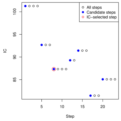
Figure 2: Two illustrations of the IC selection rule; on the left, an example in which $\mathrm{null}(D_{-\mathcal{B}_{k}})$ changes at only 6 steps (representing, e.g., the 2d fused lasso case); on the right, an example in which $\mathrm{null}(D_{-\mathcal{B}_{k}})$ changes at every step (representing, e.g., the 1d fused lasso case). In both panels, solid blue circles mark the candidate set $\widehat{I}^{\mathrm{IC}}(y)$ in (15), and a large red circle is drawn around the IC-selected step in (16).

We now show that the following set is a polyhedron in $y$,

$$H=\Big{\{}y:\widehat{M}_{1:(k_{j+q})}(y)=M_{1:(k_{j+q})},\;\hat{k}(y)=k_{j},\;\widehat{S}_{1:(j-1)}(y)=S_{1:(j-1)}\Big{\}}.$$

(By specifying $\widehat{M}_{1:(k_{j+q})}(y)=M_{1:(k_{j+q})}$, we have also implicitly specified the first $j+q$ elements of $\widehat{I}^{\mathrm{IC}}(y)$, and so we do not need to explicitly include a realization of the latter set in the definition of $H$.) In particular, we show that we can express $H=\{y:\Gamma y\geq 0,\;\Lambda y\geq w\}$, for the matrix $\Gamma=\Gamma(M_{1:k_{j+q}})$ described in the previous subsection, and for $\Lambda=\Lambda(M_{1:(k_{j}+q)},k_{j},S_{1:(j-1)})$ and $w=w(M_{1:(k_{j}+q)},k_{j},S_{1:(j-1)})$, whose construction is to be described below. Since the polyhedron (cone) $\{y:\Gamma y\geq 0\}$ characterizes the part $H_{1}=\{y:\widehat{M}_{1:(k_{j+q})}(y)=M_{1:(k_{j+q})}\}$, it suffices to study $H_{2}=\{y:\hat{k}(y)=k_{j},\;\widehat{S}_{1:(j-1)}(y)=S_{1:(j-1)}\}$, given $M_{1:(k_{j+q})}$. And as this part is defined entirely by pairwise comparisons of IC values, it suffices to show that, for any $\ell$,

$$J(M_{k_{\ell+1}})\geq J(M_{k_{\ell}})$$ (17)

is equivalent to (a pair of) linear constraints on $y$. By symmetry, if we reverse the inequality sign above, then this will still be equivalent to linear constraints on $y$, and collecting these constraints over steps $\ell=1,\ldots,j,\ldots,j+q-1$ gives the polyhedron that determines $H_{2}$. Simply recalling the IC definition in (14), and rearranging, we find that (17) is equivalent to

$$y^{T}\big{(}P_{\mathrm{null}(D_{-\mathcal{B}_{k_{\ell}}})}-P_{\mathrm{null}(D_{-\mathcal{B}_{k_{\ell+1}}})}\big{)}y\geq P_{n}\big{(}\mathrm{nullity}(D_{-\mathcal{B}_{k_{\ell}}})\big{)}-P_{n}\big{(}\mathrm{nullity}(D_{-\mathcal{B}_{k_{\ell+1}}})\big{)}.$$ (18)

Note that, by construction, the sets $\mathcal{B}_{k_{\ell}}$ and $\mathcal{B}_{k_{\ell+1}}$ differ by at most one element. For concreteness, suppose that $\mathcal{B}_{k_{\ell}}\subset\mathcal{B}_{k_{\ell+1}}$; the other direction is similar. Then $\mathrm{null}(D_{-\mathcal{B}_{k_{\ell}}})\subset\mathrm{null}(D_{-\mathcal{B}_{k_{\ell+1}}})$, and the two subspaces are of codimension 1. Further, it is not hard to see that the difference in projection operators $P_{\mathrm{null}(D_{-\mathcal{B}_{k_{\ell+1}}})}-P_{\mathrm{null}(D_{-\mathcal{B}_{k_{\ell}}})}$ is itself the projection onto a subspace of dimension 1. Writing $a_{\ell}$ for the unit-norm basis vector for this subspace, and $-b_{\ell}$ for the right hand side in (18), we see that (18) becomes

$$-(a_{\ell}^{T}y)^{2}\geq-b_{\ell},$$

or, since $b_{\ell}\geq 0$ (this is implied by $\mathrm{nullity}(D_{-\mathcal{B}_{k_{\ell+1}}})>\mathrm{nullity}(D_{-\mathcal{B}_{k_{\ell}}})$, and the complexity penalty $P_{n}$ being an increasing function),

$$-\sqrt{b_{\ell}}\leq a_{\ell}^{T}y\leq\sqrt{b_{\ell}}.$$

This is a pair of linear constraints on $y$, and we have verified the desired fact.

Altogether, with the final polyhedron $H$, we can use the TG pivot from Section 2.2 to perform valid inference on linear contrasts $v^{T}\theta$ of the mean $\theta$, conditional on having chosen step $k$ with our IC-based stopping rule, and on having observed a given model sequence over the first $k$ steps of the generalized lasso path.

3.3 What is the conditioning set?

For a fixed $k$, suppose that we have computed $k$ steps of the generalized lasso path and observed a model sequence $\widehat{M}_{1:k}(y)=M_{1:k}$. From Section 3.1, we can form a matrix $\Gamma=\Gamma(M_{1:k})$ such that $\{y:\widehat{M}_{1:k}(y)=M_{1:k}\}=\{y:\Gamma y\geq 0\}$. From Section 2.2, for any vector $v$, we can invert the TG pivot as in (13) to compute a conditional confidence interval $C_{1-\alpha}=[\delta_{\alpha},\delta_{1-\alpha/2}]$, with the property

$$\mathbb{P}\Big{(}v^{T}\theta\in C_{1-\alpha}\;\Big{|}\;\widehat{M}_{1:k}(y)=M_{1:k}\Big{)}=1-\alpha.$$ (19)

This holds for all possible realizations $M_{1:k}$ of model sequences, and thus we can marginalize along any dimension to yield a valid conditional coverage statement. For example, by marginalizing over all possible realizations $M_{1:(k-1)}$ of model sequences up to step $k-1$, we obtain

$$\mathbb{P}\Big{(}v^{T}\theta\in C_{1-\alpha}\;\Big{|}\;\widehat{\mathcal{B}}_{k}(y)=\mathcal{B}_{k},\;\hat{s}_{\mathcal{B}_{k}}(y)=s_{\mathcal{B}_{k}},\;\widehat{R}^{\mathrm{hit}}_{k}(y)=R^{\mathrm{hit}}_{k},\;\widehat{I}^{\mathrm{leave}}_{k}(y)=I^{\mathrm{leave}}_{k}\Big{)}=1-\alpha.$$ (20)

Above, $\widehat{\mathcal{B}}_{k}(y)$ is the boundary set at step $k$ as a function of $y$, and likewise $\hat{s}_{\mathcal{B}_{k}}(y),\widehat{R}^{\mathrm{hit}}_{k}(y),\widehat{I}^{\mathrm{leave}}_{k}(y)$ are the boundary signs, viable hitting signs, and viable leaving coordinates at step $k$, respectively, as functions of $y$. Since a data analyst typically never sees the viable hitting signs or viable leaving coordinates at a generalized lasso solution (i.e., these are “hidden” details of the path computation, at least compared to the boundary set and signs, which are reflected in the structure of solution itself, recall (10) and (6)), the conditioning event in (19) may seem like it includes “unnecessary” details. Hence, we can again marginalize over all possible realizations $R^{\mathrm{hit}}_{k},I^{\mathrm{leave}}_{k}$ to yield

$$\mathbb{P}\Big{(}v^{T}\theta\in C_{1-\alpha}\;\Big{|}\;\widehat{\mathcal{B}}_{k}(y)=\mathcal{B}_{k},\;\hat{s}_{\mathcal{B}_{k}}(y)=s_{\mathcal{B}_{k}}\Big{)}=1-\alpha.$$ (21)

Among (19), (20), (21), the latter is the cleanest statement and offers the simplest interpretation. This is reiterated when we cover specific problem cases in Section 4.

Similar statements hold when $k$ is chosen by our IC-based rule, from Section 3.2. Applying the TG framework from Section 2.2 to the full conditioning set, in order to derive a confidence interval $C_{1-\alpha}$ for $v^{T}\theta$, and following a reduction analogous to (19), (20), (21), we arrive at the property

$$\mathbb{P}\Big{(}v^{T}\theta\in C_{1-\alpha}\;\Big{|}\;\widehat{\mathcal{B}}_{k}(y)=\mathcal{B}_{k},\;\hat{s}_{\mathcal{B}_{k}}(y)=s_{\mathcal{B}_{k}},\;\hat{k}(y)=k\Big{)}=1-\alpha.$$ (22)

Again this is a clean conditional coverage statement and offers a simple interpretation, for $k$ chosen in a data-driven manner.

4 Special applications and extensions

4.1 Changepoint detection via the 1d fused lasso

Changepoint detection is an old topic with a vast literature. It has applications in many areas, e.g., bioinformatics, climate modeling, finance, and audio and video processing. Instead of attempting to thoroughly review the changepoint detection literature, we refer the reader to the comprehensive surveys and reviews in Brodsky & Darkhovski (1993); Chen & Gupta (2000); Eckley et al. (2011). Broadly speaking, a changepoint detection problem is one in which the distribution of observations along an ordered sequence potentially changes at some (unknown) locations. In a slight abuse of notation, we use the term changepoint detection to refer to the particular setting in which there are changepoints in the underlying mean. Our focus is on conducting valid inference related to the selected changepoints. The existing literature applicable to this goal is relatively small; is reviewed in Section 1.2 and compared to our methods in Section 5.2.

Among various methods for changepoint detection, the 1d fused lasso (Tibshirani et al., 2005), also known as 1d total variation denoising in signal processing (Rudin et al., 1992), is of particular interest because it is a special case of the generalized lasso. Let $y=(y_{1},\ldots,y_{n})$ denote values observed at $1,\dots,n$. Then the 1d fused lasso estimator is defined as in (3), with the penalty matrix being the discrete first difference operator, $D=D^{(1)}\in\mathbb{R}^{(n-1)\times n}$:

$$D^{(1)}=\left[\begin{array}[]{ccccc}-1&1&0&\ldots&0\\ 0&-1&1&\ldots&0\\ \vdots&&\ddots&\ddots&\\ 0&0&\ldots&-1&1\end{array}\right].$$ (23)

In the 1d fused lasso problem, the dual boundary set tracked by Algorithm 1 has a natural interpretation: it provides the locations of changepoints in the primal solution, which we can see more or less directly from (6) (see also Tibshirani & Taylor (2011); Arnold & Tibshirani (2016)). Therefore, we can rewrite (10) as

$$\hat{\beta}(\lambda)=\sum_{j=1}^{k+1}\hat{b}_{j}(\lambda)\,\mathds{1}_{(I_{j-1}+1):I_{j}},\quad\text{for $\lambda\in[\lambda_{k+1},\lambda_{k}]$}.$$ (24)

Here $I_{1}<\ldots<I_{k}$ denote the sorted elements of the boundary set $\mathcal{B}_{k}$, with $I_{0}=0$, $I_{k+1}=n$ for convenience, $\mathds{1}_{p:q}$ denotes a vector with 1 in positions $p\,\dots q$ and 0 elsewhere, and $\hat{b}_{1}(\lambda),\ldots,\hat{b}_{k+1}(\lambda)$ denote levels estimated by the fused lasso with parameter $\lambda$. Note that in (24), we have implicitly used the fact that the boundary set after $k$ steps of the path algorithm has exactly $k$ elements; this is true since the path algorithm never deletes coordinates from the boundary set in 1d fused lasso problems (as mentioned following Algorithm 1). The dual boundary signs also have a natural meaning: writing the elements of $s_{\mathcal{B}_{k}}$ as $s_{I_{1}},\ldots,s_{I_{k}}$, these record the signs of differences (or jumps) between adjacent levels,

$$\mathrm{sign}\big{(}\hat{b}_{j+1}(\lambda)-\hat{b}_{j}(\lambda)\big{)}=s_{I_{j}},\quad\text{for $j=1,\ldots,k$, $\lambda\in[\lambda_{k+1},\lambda_{k}]$}.$$ (25)

Below, we describe several aspects of selective inference with 1d fused lasso estimates. Similar discussions could be given for the different special classes of generalized lasso problems, like trend filtering and the graph fused lasso, but for brevity we only go into such detail for the 1d fused lasso.

Contrasts for the fused lasso.

The framework laid out in Section 3 allows us to perform post-selection TG tests for hypotheses about $v^{T}\theta$, for any contrast vector $v$. We introduce two specific forms of interesting contrasts, which we call the segment and spike contrasts. From the $k$-step fused lasso solution, as portrayed in (24), (25), there are two natural questions one could ask about the changepoint $I_{j}$, for some $j\in\{1,\dots,k\}$: first, whether there is a difference in the underlying mean exactly at $I_{j}$,

$$H_{0}:\theta_{I_{j}+1}=\theta_{I_{j}}\quad\text{versus}\quad H_{1}:s_{I_{j}}(\theta_{I_{j}+1}-\theta_{I_{j}})>0.$$ (26)

and second, whether there is an average difference in the mean between the regions separated by $I_{j}$,

$$H_{0}:\bar{\theta}_{(I_{j}+1):I_{j+1}}=\bar{\theta}_{(I_{j-1}+1):I_{j}}\quad\text{versus}\quad H_{1}:s_{I_{j}}(\bar{\theta}_{(I_{j}+1):I_{j+1}}-\bar{\theta}_{(I_{j-1}+1):I_{j}})>0.$$ (27)

These hypotheses are fundamentally different: that in (26) is sensitive to the exact location of the underlying mean difference, whereas that in (27) can be non-null even if the change in mean is not exactly at $I_{j}$. To test (26), we use the so-called spike contrast

$$v_{\mathrm{spike}}=s_{I_{j}}(\mathds{1}_{I_{j}+1}-\mathds{1}_{I_{j}}).$$ (28)

The resulting TG test, as in (12) with $v=v_{\mathrm{spike}}$, is called the spike test, since it tests differences in the mean $\theta$ at exactly one location. To test (27), we use the so-called segment contrast

$$v_{\mathrm{seg}}=s_{I_{j}}\bigg{(}\frac{1}{I_{j+1}-I_{j}}\mathds{1}_{(I_{j}+1):I_{j+1}}-\frac{1}{I_{j}-I_{j-1}}\mathds{1}_{(I_{j-1}+1):I_{j}}\bigg{)}.$$ (29)

The resulting TG test, as in (12) with $v=v_{\mathrm{seg}}$, is called the segment test, because it tests average differences across segments of the mean $\theta$.

In practice, the segment test often has more power than the spike test to detect a change in the underlying mean, since it averages over entire segments. However, it is worth pointing out that the usefulness of the segment test at $I_{j}$ also depends on the quality of the other detected changepoints 1d fused lasso model (unlike the spike test, which does not), because these determine the lengths of the segments drawn out on either side of $I_{j}$. And, to emphasize what has already been said: unlike the spike test, the segment test does not test the precise location of a changepoint, so a rejection of its null hypothesis must not be mistakenly interpreted (also, refer to the corresponding coverage statement in (30)).

Which test is appropriate ultimately depends on the goals of the data analyst. Figure 3 shows a simple example of the spike and segment tests. The behaviors of these two tests will be explored more thoroughly in Section 5.1.

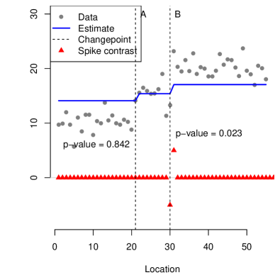
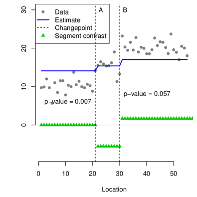
Figure 3: An example with $n=60$ points, portraying the differences between the spike and segment tests for the fused lasso. The underlying mean has true changepoints at locations 20 and 30; the 2-step fused lasso estimate, drawn in blue, detects changepoints at locations 21 and 30, labeled $A$ and $B$. P-values from the segment test are reported in the left panel, and from the spike test in the right panel. The segment and spike contrast vectors around changepoint $B$ are visualized on the panels (the entries of these vectors have been scaled up for visibility). We can see that both segment p-values are small, and both segment null hypotheses defined around locations $A$ and $B$ should be rejected; but only the spike p-value at location $B$ is small, and only the the spike null hypothesis around location $B$ should be rejected (as location $A$ does not correspond to a true changepoint in the underlying mean).

Alternative motivation for the contrasts.

It may be interesting to note that, for the segment contrast $v_{\mathrm{seg}}$ in (29), the statistic

$$v_{\mathrm{seg}}^{T}y=\bar{y}_{(I_{j}+1):I_{j+1}}-\bar{y}_{(I_{j-1}+1):I_{j}}$$

is the likelihood ratio test statistic for testing the null $H_{0}:\theta_{I_{j-1}+1}=\ldots=\theta_{I_{j}}=\theta_{I_{j}+1}=\ldots=\theta_{I_{j+1}}$ versus the alternative $H_{1}:\theta_{I_{j-1}+1}=\ldots=\theta_{I_{j}}\not=\theta_{I_{j}+1}=\ldots=\theta_{I_{j+1}}$, if the locations $I_{j-1},I_{j},I_{j+1}$ were fixed. An equivalent way to write these hypotheses, which will be a helpful generalization going forward (as we consider other classes of generalized lasso problems), is

$$H_{0}:\theta\in\mathrm{null}(D_{-\mathcal{B}_{k}})\quad\text{versus}\quad H_{1}:\theta\in\mathrm{null}(D_{-\mathcal{B}_{k}\setminus\{I_{j}\}}).$$

In this notation, the segment contrast $v_{\mathrm{seg}}$ in (29) is the unique (up to a scaling factor) basis vector for the rank 1 subspace $\mathrm{null}(D_{-\mathcal{B}_{k}})\setminus\mathrm{null}(D_{-\mathcal{B}_{k}\setminus\{I_{j}\}})=\mathrm{null}(D_{-\mathcal{B}_{k}\setminus\{I_{j}\}})^{\perp}\mathrm{null}(D_{-\mathcal{B}_{k}})$, and $v_{\mathrm{seg}}^{T}y$ is the likelihood ratio test statistic for the above set of null and alternative hypotheses.

Lastly, both segment and spike tests can be viewed from an equivalent regression perspective, after transforming the 1d fused lasso problem in (3), (23) into an equivalent lasso problem (recall Section 2.3). In this context, it can be shown that the segment test corresponds to a test of a partial regression coefficient in the active model, whereas the spike test corresponds to a test of a marginal regression coefficient.

Inference with an interpretable conditioning event.

As explained in Section 3.3, there are different levels of conditioning that can be used to interpret the results of the TG tests for model selection events along the generalized lasso path. Here we demonstrate for the segment test in (27), (29) what we see as the simplest interpretation of its conditional coverage property, with respect to its parameter $\bar{\theta}_{(I_{j}+1):I_{j+1}}-\bar{\theta}_{(I_{j-1}+1):I_{j}}$. The TG interval $C_{1-\alpha}=[\delta_{\alpha},\delta_{1-\alpha/2}]$ in (13), computed by inverting the TG pivot, has the exact finite sample property

$$\mathbb{P}\Big{(}\bar{\theta}_{(I_{j}+1):I_{j+1}}-\bar{\theta}_{(I_{j-1}+1):I_{j}}\in C_{1-\alpha}\;\Big{|}\;I_{1},\ldots,I_{k},s_{I_{1}},\ldots,s_{I_{k}}\Big{)}=1-\alpha,$$ (30)

obtained by marginalizing over some dimensions of the conditioning set, as done in Section 3.3. In words, the coverage statement (30) says that, conditional on the estimated changepoints $I_{1},\ldots,I_{k}$ and estimated jump signs $s_{I_{1}},\ldots,s_{I_{k}}$ in the $k$-step 1d fused lasso solution, the interval $C_{1-\alpha}$ traps the jump in segment averages $\bar{\theta}_{(I_{j}+1):I_{j+1}}-\bar{\theta}_{(I_{j-1}+1):I_{j}}$ with probability $1-\alpha$. This all assumes that the choice of step $k$ is fixed; for $k$ chosen by an IC-based rule as described in Section 3.2, the interpretation is very similar and we only need to add $k$ to the right-hand side of the conditioning bar in (30). A similar interpretation is also available for the spike test, which we omit for brevity.

One-sided or two-sided inference?

We note that both setups in (26) and (27) use a one-sided alternative hypothesis, and the contrast vectors in (28) and (29) are defined accordingly. To put it in words, we are testing for changepoint in the underlying mean $\theta$ (either exactly at one location, or in an average sense across local segments) and are looking to reject when a jump in $\theta$ occurs in the direction we have already observed in the fused lasso solution, as dictated by the sign $s_{I_{j}}$. On the other hand, for coverage statements as in (30), we are implicitly using a two-sided alternative, replacing the alternative in (27) by $H_{1}:\bar{\theta}_{(I_{j}+1):I_{j+1}}\not=\bar{\theta}_{(I_{j-1}+1):I_{j}}$ (since the coverage interval is the result of inverting a two-sided pivotal statistic). Two-sided tests and one-sided intervals are also possible in our inference framework, however, we find them less natural, and our default is therefore to consider the aforementioned versions.

4.2 Knot detection via trend filtering

Trend filtering can be seen as an extension of the 1d fused lasso for fitting higher-order piecewise polynomials (Steidl et al., 2006; Kim et al., 2009; Tibshirani, 2014). It can be defined for any desired polynomial order, written as $r\geq 0$, with $r=0$ giving piecewise constant segments and reducing to the 1d fused lasso of the last subsection. Here we focus on the case $r=1$, where piecewise linear segments are fitted. The general case $r\geq 2$ is possible by following the exact same logic, though for simplicity, we do not cover it.

As before, we assume the data $y=(y_{1},\ldots,y_{n})$ has been measured at ordered locations $1,\ldots,n$. The linear trend filtering estimate is defined as in (3) with $D=D^{(2)}\in\mathbb{R}^{(n-2)\times n}$, the discrete second difference operator:

$$D^{(2)}=\left[\begin{array}[]{cccccc}1&-2&-1&0&\ldots&0\\ 0&1&-2&1&\ldots&0\\ \vdots&&\ddots&\ddots&\ddots&\\ 0&0&\ldots&1&-2&1\end{array}\right].$$ (31)

For the linear trend filtering problem, the elements of the dual boundary set are in one-to-one correspondence with knots, i.e., changes in slope, in the piecewise linear sequence $\hat{\beta}=(\hat{\beta}_{1},\ldots,\hat{\beta}_{n})$. This comes essentially from (6) (for more, see Tibshirani & Taylor (2011); Arnold & Tibshirani (2016)). Specifically, enumerating the elements of the boundary set $\mathcal{B}_{k}$ as $I_{1}<\ldots<I_{q}$ (and using $I_{0}=0$ and $I_{q+1}=0$ for convenience), each location $I_{j}+1$, $j=1,\ldots,q$ serves a knot in the trend filtering solution, so that we may rewrite (10) as

$$\hat{\beta}(\lambda)=\sum_{j=1}^{q+1}\Big{(}\hat{b}_{j}(\lambda)+\hat{m}_{j}(\lambda)(j-I_{j-1}-1)\Big{)}\mathds{1}_{(I_{j-1}+1):I_{j}},\quad\text{for $\lambda\in[\lambda_{k+1},\lambda_{k}]$}.$$ (32)

Above, $q$ denotes the number of knots in the $k$-step linear trend filtering solution, which in general need not be equal to $k$, since (unlike the 1d fused lasso) the path algorithm for linear trend filtering can both add to and delete from the boundary set at each step. Also, for each $j=1,\ldots,q+1$, the quantities $\hat{b}_{j}(\lambda)$ and $\hat{m}_{j}(\lambda)$ denote the “local” intercept and slope parameters, respectively, of the linear trend filtering solution, over the segment $\{I_{j-1}+1,\ldots,I_{j}\}$. Denoting the dual boundary signs $s_{\mathcal{B}_{k}}$ by $s_{I_{1}},\ldots,s_{I_{q}}$, we have

$$\mathrm{sign}\big{(}\hat{m}_{j+1}(\lambda)-\hat{m}_{j}(\lambda)\big{)}=s_{I_{j}},\quad\text{for $j=1,\ldots,q$, $\lambda\in[\lambda_{k+1},\lambda_{k}]$},$$ (33)

i.e., these signs of changes in slopes between adjacent trend filtering segments.

Contrasts for linear trend filtering.

We can construct both spike and segment tests for linear trend filtering using similar motivations as in the 1d fused lasso. Given the trend filtering solution in (32), (33), we consider testing a particular knot location $I_{j}+1$, for some $j=1,\ldots,q$. The spike contrast is defined by

$$v_{\mathrm{spike}}=s_{I_{j}}(\mathds{1}_{I_{j}}-2\mathds{1}_{I_{j}+1}+\mathds{1}_{I_{j}+2}),$$ (34)

and the TG statistic in (12) with $v=v_{\mathrm{spike}}$ provides us with a test for

$$H_{0}:\theta_{I_{j}+1}=\frac{\theta_{I_{j}}+\theta_{I_{j}+2}}{2}\quad\text{versus}\quad H_{1}:s_{I_{j}}(\theta_{I_{j}}-2\theta_{I_{j}+1}+\theta_{I_{j}+2})>0.$$ (35)

The segment contrast is harder to define explicitly from first principles, but can be defined following one of the alternative motivations for the segment contrast in the 1d fused lasso problem: consider the rank 1 subspace $\mathrm{null}(D_{-\mathcal{B}_{k}})\setminus\mathrm{null}(D_{-\mathcal{B}_{k}\setminus\{I_{j}\}})=\mathrm{null}(D_{-\mathcal{B}_{k}\setminus\{I_{j}\}})^{\perp}\mathrm{null}(D_{-\mathcal{B}_{k}})$, and define $w$ to be a basis vector for this subspace (unique up to scaling). The segment contrast is then

$$v_{\mathrm{seg}}=\mathrm{sign}(w_{I_{j}}-2w_{I_{j}+1}+w_{I_{j}+2})s_{I_{j}}w,$$ (36)

i.e., we align $w$ so that its second difference around the knot $I_{j}+1$ matches that in the trend filtering solution. To test $v_{\mathrm{seg}}^{T}\theta=0$, we can use the TG statistic in (12) with $v=v_{\mathrm{seg}}$; however, as $w$ is not easy to express in closed-form, this null hypothesis is also not easy to express in closed-form. Still, we can rewrite it in a slightly more explicit manner:

$$H_{0}:h^{T}(\theta-\theta^{\mathrm{proj}})=0\quad\text{where}\quad h=(\underbrace{0,\ldots,0}_{I_{j}+1},\underbrace{1,2,3,\ldots,n-I_{j}-2}_{n-I_{j}-1})\;\,\text{and}\;\,\theta^{\mathrm{proj}}=P_{\mathrm{null}(D_{-\mathcal{B}_{k}\setminus\{I_{j}\}})}\theta,$$ (37)

versus the appropriate one-sided alternative hypothesis. In words, $\theta^{\mathrm{proj}}$ is the projection of $\theta$ onto the space of piecewise linear vectors with knots at locations $I_{\ell}+1$, $\ell\not=j$, and $h$ is a single piecewise linear activation vector that rises from zero at location $I_{j}+1$.

The same high-level points comparing the spike and segment tests for the fused lasso also carry over to the linear trend filtering problem: the segment test can often deliver more power, but at a given location $I_{j}+1$, the power of the segment test will depend on the other knot locations in the estimated model. The spike test at location $I_{j+1}$ does not depend on any other knot points in the trend filtering solution. Furthermore, the segment null does not specify a precise knot location, and one must be careful in interpreting a rejection here. Figure 4 gives examples of the segment test for linear trend filtering. More examples are investigated in Section 5.3.

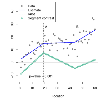
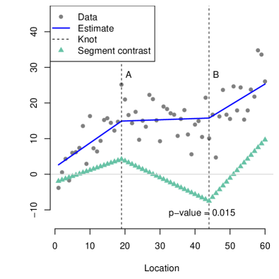
Figure 4: An example with $n=60$ points, portraying two segment tests for trend filtering. The underlying piecewise linear mean has knots at locations 20 and 40; the 2-step linear trend filtering estimate, in blue, detects knots at locations 17 and 39, labeled A and B. The left plot shows the result the segment test at knot A, and the right plot at knot B. In each, the segment contrast is visualized. Both p-values are small.

4.3 Cluster detection via the graph fused lasso

The graph fused lasso is another generalization of the 1d fused lasso, in which we depart from the 1-dimensional ordering of the components of $y=(y_{1},\ldots,y_{n})$. Now we think of these components as being observed over nodes $V=\{1,\ldots,n\}$ of a given (undirected) graph, with edges $E=\{e_{1},\ldots,e_{m}\}$, where say each $e_{\ell}=(i_{\ell},j_{\ell})$ joins some nodes $i_{\ell}$ and $j_{\ell}$, for $\ell=1,\ldots,m$. Note that the 1d fused lasso corresponds to the special case in which $E=\{(i,i+1):i=1,\ldots,n\}$, called the chain graph. For a general graph $G=(V,E)$, we define its edge incidence matrix $D_{G}\in\mathbb{R}^{m\times n}$ by having rows of the form

$$D_{\ell}=(0,\ldots\underset{\begin{subarray}{c}\;\;\uparrow\\ \;\;i_{\ell}\end{subarray}}{-1},\ldots\underset{\begin{subarray}{c}\uparrow\\ j_{\ell}\end{subarray}}{1},\ldots 0),$$ (38)

when the $\ell$th edge is $e_{\ell}=(i_{\ell},j_{\ell})$, with $i_{\ell}<j_{\ell}$, for $\ell=1,\ldots,m$. The graph fused lasso problem, also called graph total variation denoising, is given by (3) with $D=D_{G}$. This has been studied by many authors, particularly in the case when $G$ is a 2-dimensional grid, and the resulting program, called the 2d fused lasso, is useful for image denoising (see, e.g., Friedman et al. (2007); Chambolle & Darbon (2009); Hoefling (2010); Tibshirani & Taylor (2011); Sharpnack et al. (2012); Arnold & Tibshirani (2016)). Trend filtering can also be extended to graphs (Wang et al., 2016); in principle our inferential treatment here extends to this problem as well, though we do not discuss it.

The boundary set constructed by the dual path algorithm, Algorithm 1, has the following interpretation for the graph fused lasso problem (Tibshirani & Taylor, 2011; Arnold & Tibshirani, 2016). Denoting $\mathcal{B}_{k}=\{I_{1},\ldots,I_{q}\}$, each element $I_{\ell}$ corresponds to an edge $e_{I_{\ell}}$ in the graph, $\ell=1,\ldots,q$. The graph fused lasso solution is then piecewise constant over the sets $C_{1},\ldots,C_{p}$, which form partition of $\{1,\ldots,n\}$, and are defined by the connected components of $G=(V,E\setminus\{e_{I_{\ell}}:\ell,\ldots,q\})$, i.e., the original graph with the edges $e_{I_{\ell}}$, $\ell=1,\ldots,q$ removed. That is, we may express (10) as

$$\hat{\beta}(\lambda)=\sum_{j=1}^{p}\hat{b}_{j}(\lambda)\mathds{1}_{C_{j}},\quad\text{for $\lambda\in[\lambda_{k+1},\lambda_{k}]$},$$ (39)

where $p$ denotes the number of connected components, $\mathds{1}_{C_{j}}$ denotes the indicator vector $C_{j}$, having $i$th entry 1 if $i\in C_{j}$ and 0 otherwise, and $\hat{b}_{j}(\lambda)$ denotes an estimated level for component $C_{j}$, for $j=1,\ldots,p$. The dual boundary signs $s_{\mathcal{B}_{k}}=\{s_{I_{1}},\ldots,s_{I_{q}}\}$, capture the signs of differences between levels in the graph fused lasso solution,

$$\mathrm{sign}\big{(}\hat{\beta}_{j_{\ell}}(\lambda)-\hat{\beta}_{i_{\ell}}(\lambda)\big{)}=s_{I_{\ell}},\quad\text{when $e_{I_{\ell}}=(i_{\ell},j_{\ell})$, with $i_{\ell}<j_{\ell}$,}\\ \text{for $\ell=1,\ldots,q$, and $\lambda\in[\lambda_{k+1},\lambda_{k}]$}.$$ (40)

Contrasts for the graph fused lasso.

For the graph fused lasso problem, it is more natural to consider segment (rather than spike) type contrasts, conforming with the notation and concepts introduced for the 1d fused lasso problem. Even restricting our attention to segments tests, many possibilities are available to us, given the graph fused lasso solution as in (39), (40). Say, we may choose any two “neighboring” connected components $C_{a}$ and $C_{b}$, for some $a,b=1,\ldots,p$, meaning that there exists at least one edge (in the original graph) between $C_{a}$ and $C_{b}$, and test

$$H_{0}:\bar{\theta}_{C_{a}}=\bar{\theta}_{C_{b}}\quad\text{versus}\quad H_{1}:s_{ab}(\bar{\theta}_{C_{b}}-\bar{\theta}_{C_{a}})>0,$$ (41)

where $s_{ab}=s_{I_{\ell}}$, for some element $I_{\ell}\in\mathcal{B}_{k}$ such that $e_{I_{\ell}}=(i_{\ell},j_{\ell})$, with $i_{\ell}<j_{\ell}$, and $i_{\ell}\in C_{a}$, $j_{\ell}\in C_{b}$. Above, we use the notation $\bar{\theta}_{S}=\sum_{i\in S}\theta_{i}/|S|$ for a subset $S$. The hypothesis in (41) tests whether the average of $\theta$ over components $C_{a}$ and $C_{b}$ are equal, versus the alternative that they differ and their difference matches the sign witnessed in the graph fused lasso solution. To test (41), we can use the TG statistic in (12) with $v=v_{\mathrm{seg}}$, where

$$v_{\mathrm{seg}}=s_{ab}\bigg{(}\frac{1}{|C_{b}|}\mathds{1}_{C_{b}}-\frac{1}{|C_{a}|}\mathds{1}_{C_{a}}\bigg{)}.$$ (42)

As in the 1d fused lasso problem, the above contrast can also be motivated by the fact that $v_{\mathrm{seg}}^{T}y$ is the likelihood ratio test for an appropriate pair of null and alternative hypotheses. More advanced segment tests are also possible, say, by testing whether averages of $\theta$ are equal over two subsets, each given by a union of connected components among $C_{1},\ldots,C_{q}$. Figure 5 shows a simple example of a segment test of the form (41), (42) for the graph fused lasso. Section 5.4 gives another example.

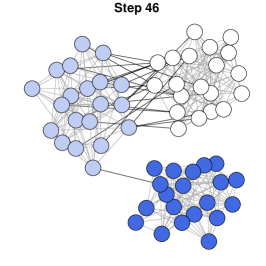
Figure 5: An example with $n=60$ nodes illustrating the segment test for the graph fused lasso. The graph was generated using a simple stochastic block model with 3 groups of 20 nodes each. The edge probabilities were 0.5 for nodes in the same group and 0.05 for nodes in different groups. This resulted in $m=369$ edges. The group means were defined to be 0, 1, and 3 (colored in white, light blue, and dark blue, above). Data were generated by adding i.i.d. centered Gaussian noise, with standard deviation 0.15. The left plot displays the initial graph, with 321 total edges. The middle plot displays the graph fused lasso estimate after 46 path steps, where there is only one edge left separating group 3 from groups 1 and 2. At step 47, in the right plot, this last edge is removed and the segment test (41), (42) is applied, with $C_{a}$ being the union of groups 1 and 2 (white and light blue) and $C_{b}$ being group 3 (dark blue). The p-value is small, around $0.03$.

4.4 Problems with additional sparsity

The generalized lasso signal approximator problem in (3) can be modified to impose pure sparsity regularization on $\beta$ itself, as in

$$\hat{\beta}=\mathop{\mathrm{argmin}}_{\beta\in\mathbb{R}^{n}}\;\frac{1}{2}\|y-\beta\|_{2}^{2}+\lambda\|D\beta\|_{1}+\alpha\lambda\|\beta\|_{1},$$ (43)

where $\alpha\geq 0$ is an another tuning parameter. The above may be called the sparse generalized lasso signal approximation problem. In fused lasso settings, both 1d and graph-based, the estimate $\hat{\beta}$ in (43) will now be piecewise constant across its components, with many attained levels being equal to zero exactly (for a large enough value of $\alpha>0$). In fact, the fused lasso as originally defined by Tibshirani et al. (2005) was just as in (43), with both fusion and sparsity penalties. In trend filtering settings, the estimate $\hat{\beta}$ in (43) will be similar, except that it will now have a piecewise polynomial structure whenever it is nonzero. There are many examples in which pure sparsity regularization is a useful addition, see Section 5.6, and also, e.g., Tibshirani et al. (2005); Friedman et al. (2007); Tibshirani & Wang (2008); Tibshirani (2014).

Of course, problem (43) is still a generalized lasso problem, since the two penalty terms in the criterion can be represented by $\lambda\|\tilde{D}\beta\|_{1}$, where $\tilde{D}\in\mathbb{R}^{(m+n)\times n}$ is given by row-binding $D\in\mathbb{R}^{m\times n}$ and $\alpha I\in\mathbb{R}^{n\times n}$. This means that all the tools presented so far in this paper are applicable, and post-selection inference can be performed for problems like the sparse fused lasso and sparse trend filtering.

4.5 Generalized lasso regression problems

Up until this point, our applications have focused on the signal approximation problem in (3), but all of our methodology carries over to the generalized lasso regression problem in (2). Allowing for a general regression matrix $X\in\mathbb{R}^{n\times p}$ greatly extends the scope of applications; see Section 5.5, and the discussions and examples in, e.g., Tibshirani et al. (2005); Friedman et al. (2007); Tibshirani & Taylor (2011); Arnold & Tibshirani (2016).

To tackle the regression problem in (2) with our framework, we must assume that $\mathrm{rank}(X)=p$ (which requires $n\geq p$). We follow the transformation suggested by Tibshirani & Taylor (2011),

$$\hat{\beta}=\mathop{\mathrm{argmin}}_{\beta\in\mathbb{R}^{p}}\;\frac{1}{2}\|y-X\beta\|_{2}^{2}+\lambda\|D\beta\|_{1}\quad\iff\quad\hat{\theta}=\mathop{\mathrm{argmin}}_{\theta\in\mathbb{R}^{n}}\;\frac{1}{2}\|\tilde{y}-\theta\|_{2}^{2}+\lambda\|\tilde{D}\theta\|_{1},$$

where $\tilde{y}=XX^{+}y$, $\tilde{D}=DX^{+}$, and the equivalence between solutions $\hat{\beta},\hat{\theta}$ is $\hat{\theta}=X\hat{\beta}$. From what we can see above, a generic generalized lasso regression problem can be transformed into a generalized lasso signal approximation problem (just with a modified response vector $\tilde{y}$ and penalty matrix $\tilde{D}$) and so all of our tools can be applied to this transformed signal approximation problem in order to perform inference.

When $\mathrm{rank}(X)<p$ (which always happens in the high-dimensional case $n<p$), we can simply add a small ridge penalty, which brings us back to the case in which the effective regression matrix is full column rank (see Tibshirani & Taylor (2011)). Then the above transformation can be applied.

4.6 Post-processing and visual aids

We briefly discuss two extensions for the post-selection inference workflow.

Post-processing.

The choices of contrasts outlined in Sections 4.1–4.5 are defined automatically from the generalized lasso selected model. Given such a selected model, before we test a hypothesis or build a confidence interval, we can optionally choose to ignore or change some of the components of the selected model, in defining a contrast of interest. We refer to this as “post-processing”; to be clear, it only affects the contrast vector being used, and not the conditioning set in any way.

It helps to give specific examples. In the 1d fused lasso problem, empirical examples reveal that the estimator sometimes places several small jumps close to one larger jump. The practitioner could choose to merge nearby jumps before forming the segment contrast of Section 4.1; we can see from (29) that this would correspond to extending the segment lengths on either side of the breakpoint in question, which could result in greater power to detect a change in the underlying mean. See the left panel of Figure 6 for an example. In trend filtering, a practitioner could also choose to merge nearby knots before forming the segment contrast in (36), from Section 4.2. See the right panel of Figure 6 for an example. Similar post-processing ideas could be carried out for the graph fused lasso and generalized lasso regression problems.

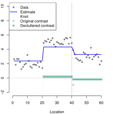
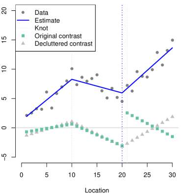
Figure 6: Examples showing the segment test contrasts before and after post-processing or “decluttering” for the 1d fused lasso, in the left panel, and trend filtering, in the right panel. In both problems, the p-values for testing at locations marked by blue dashed vertical lines dropped considerably; on the left, the p-value dropped from 0.236 to $<$0.001, and on the right, from 0.09 to 0.001. For trend filtering, it can also be demonstrated that decluttering at one location helps the power for testing at another location that is farther away, but this phenomenon is absent in the fused lasso case (due to of the finite support of the segment test contrasts).

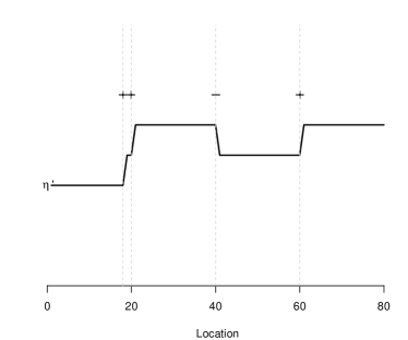
Figure 7: An example showing a 1d fused lasso solution after 4 steps, in the left panel, and its corresponding step-sign plot, in the right panel. Based on the step-sign plot, the data analyst may, e.g., deem locations 18 and 20 to be too close to be both interesting, and merge them before conducting segment tests.

Visual aids.

In designing contrasts, the data analyst may also benefit from visualization of the generalized lasso selected model. Such a “visual aid” has a similar goal to that of post-processing, namely, to improve the quality of the question asked, i.e., the hypothesis tested, following a generalized lasso selection event. For the eventual inferences to be valid, the visual aid must not reveal information about the data $y$ that is not contained in the selection event, $\widehat{M}_{1:k}(y)=M_{1:k}$, defined in Section 3.1 (assuming a fixed step number $k$, for simplicity). Again, it helps to consider the fused lasso as a specific use case. See Figure 7 for an example. We cannot, e.g., reveal the 4-step fused lasso solution to the analyst, ask him/her to hand-craft a contrast to be tested, and then expect type I error control after applying our post-selection inference tools. This is because the solution itself contains information about the data not contained in the selection event—the magnitudes of the fitted jumps—and the decision of which contrast to test could likely be affected by this information. This makes the conditioning set incomplete (said differently, it means that the contrast vector no longer measurable with respect to the conditioning event), and we should not expect our previously established inference guarantees to apply, as a result. We can, however, reveal a characature of the solution, as long as this characature is based entirely on the selection event. For the 1d fused lasso, this means that the characature must be defined in terms of the changepoint locations and signs of the fitted jumps, and we refer to it as a “step-sign plot”. Examination of the jump locations and signs can aid the analyst in designing interesting contrasts to test.

5 Empirical examples

5.1 1d fused lasso examples

One-jump signal.

First, we examine a problem setup with $n=60$, and where $\theta\in\mathbb{R}^{60}$ has one changepoint at location 30, of height $\delta$. Data $y\in\mathbb{R}^{60}$ were generated by adding i.i.d. $\mathcal{N}(0,1)$ noise to $\theta$. We considered three settings for the signal strength: $\delta=0$ (no signal), $\delta=1$ (moderate signal), and $\delta=2$ (strong signal). See the top left panel of Figure 8 for an example. Over 10,000 repetitions of the data generation process, we fit the 1-step fused lasso estimate, and computed both the spike and segment tests at the detected changepoint location. Their p-values are displayed via QQ plots, in the top middle and top right panels of Figure 8, restricted to repetitions for which the detected location was 30. (This corresponded to roughly 2.2%, 30%, and 65% of the 10,000 total trials when $\delta=0$, 1, and 2, respectively.) When $\delta=0$, we see that both the spike and segment tests deliver uniform p-values, as they should. When $\delta=1$ and 2, we see that the segment test provides much better power than the segment test, and has essentially full power at the strong signal level $\delta=2$.

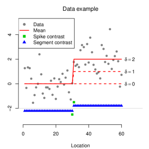
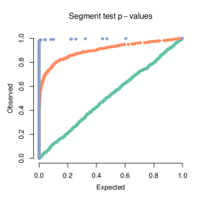
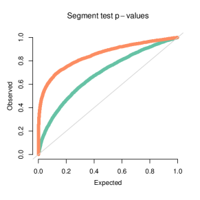
Figure 8: Examination of p-values coming from the spike and segment tests, in a setup with $n=60$ points and one or two true changepoints, shown in the top and bottom rows, respectively. In the one-jump setting, we considered three signal strengths: $\delta=0,1,2$. The top left panel shows an example simulated data set from a one-jump signal with height $\delta=2$, and the middle and right panels show the p-values from the spike and segment tests, collected over simulations for which the 1-step fused lasso correctly detected a changepoint at location 30. We can see that the segment test generally has much better power. In the two-jump setting, we only considered the signal strength of $\delta=2$, and the bottom left panel shows an example simulated data set. The middle and right panels show p-values coming from the spike and segment tests, after 1 or 2 steps of the fused lasso. At both steps, the spike and segment tests were used to test the significance of location 20. The p-values at step 1 were collected over simulations in which location 20 was detected, and at step 2 over simulations in which locations 20 and 40 were detected (in either order). We can see that the power of the segment test improves after 2 steps, as it uses a more effective contrast, but that of the spike test degrades, as it uses the same contrast and simply incurs more conditioning.

When the fused lasso detects a changepoint at location 29 or 31, i.e., a location that is off by one from the true changepoint at location 30, the spike and segment tests again perform very differently. The spike test yields uniform p-values, as it should, while the segment test offers nontrivial power. See Appendix A for QQ plots of these results.

Two-jump signal.

Next, we examine a problem with $n=60$ and where $\theta\in\mathbb{R}^{60}$ has two changepoints, at locations 20 and 40, each of height $\delta=2$. Data $y\in\mathbb{R}^{60}$ were again generated around $\theta$ by adding i.i.d. $\mathcal{N}(0,1)$ noise. See the bottom left panel of Figure 8 for an example. Over 10,000 repetitions, we fit 2 steps of the fused lasso and recorded spike and segment p-values, at each step, for testing the significance of location 20. The bottom middle and bottom right panels of Figure 8 display QQ plots, restricted at step 1 to simulations in which location 20 was detected (corresponding to about 32% of the total number of simulations), and restricted at step 2 to simulations in which locations 20 and 40 were detected (in either order, corresponding to again about 32% of the total simulations). We see that the spike test has better power at step 1 versus step 2, however, for the segment test, the story is reversed. The spike test contrast for testing at location 20 does not change between steps 1 and 2; the extra conditioning incurred at step 2 only hurts its power. On the other hand, the segment test uses a different contrast between steps 1 and 2, and the contrast at step 2 provides better power, because it leads to an average over a shorter segment (to the right of location 20) over which the mean is truly constant.

IC-based stopping rules.

The left panel of Figure 9 shows the segment test applied to a one-jump signal of length $n=20$, with a jump at location 10 of height $\delta$, but this time incorporating the IC-based stopping rules (to determine where along the fused lasso solution path to perform the test). This is a more practical performance gauge because it requires minimal user input on model selection. Shown are power curves (fraction of rejections, at the 0.05 level of type I error control) as functions of $\delta$, computed over p-values from simulations in which location 10 was detected in the final model selected by the AIC- or BIC-type rule described in Section 3.2, with $q=2$ (i.e., stopping after 2 rises in the criterion). Note that the p-values here were all adjusted by the number of changepoints in the final AIC- or BIC-selected model, using a Bonferroni correction (so that the familywise type I error is under control). The BIC-type rule has better power than the AIC-type rule, as the latter leads to larger models (AIC stops at 2.5 steps on average versus 1.7 from BIC), resulting in further conditioning and also misleading additional detected locations, both of which hurt its performance.

The results are compared to those from the segment test carried out at the 1-step fused lasso solution, over p-values from simulations in which location 10 was detected. With less conditioning (and no need for multiplicity correction), this method dominates the IC-based rules in terms of power. The results are also compared to an oracle rule who knows the correct segments and carries out a test for equality of means (with no conditioning); this serves as an upper bound for what we can expect from our methods. The right panel of Figure 9 shows BIC power curves as the sample size $n$ increases from 20 to 80, in increments of 20. We see a uniform improvement in power across all signal strengths $\delta$, as $n$ increases. However, at $n=80$, the BIC-based test still delivers a power that is noticeably worse than that of the oracle rule at $n=20$.

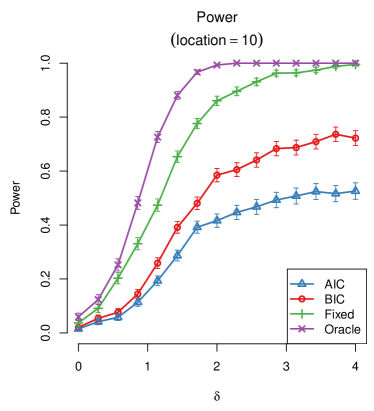
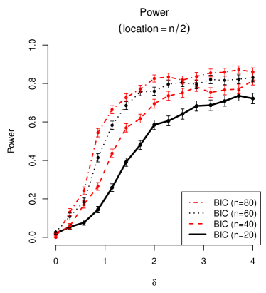
Figure 9: Power curves for a one-jump signal with $n=20$ points on the left, and $n=20,40,60,80$ on the right, and in each case, having a jump at location $n/2$, of height $\delta$. The left panel shows the results from the segment test, either at step 1 (labeled “Fixed”, in green), or at a step selected by the 2-rise AIC or BIC rule (labeled “AIC” and “BIC”, in blue and red, respectively). The power curves were computed from p-values over simulations in which location 10 appeared in the selected model (and the AIC- and BIC-based rules applied appropriate corrections for multiplicity). The left panel also shows the results of applying an oracle test at location 10, for equality of means. We can see a clear drop in power from the oracle to the fixed rule to the IC-based rules. The right panel shows the improvement in BIC power curves as $n$ increases.

5.2 Comparison to SMUCE-based inference

Here we compare our post-selection confidence intervals for the 1d fused lasso to those based on the Simultaneous Multiscale Changepoint Estimator (SMUCE) of Frick et al. (2014). The SMUCE approach provides a simultaneous confidence band for the components of the mean vector $\theta$, from which confidence intervals for any linear contrast of the mean can be obtained, and therefore, valid confidence intervals for post-selection targets can be obtained. Admittedly, a simultaneous band is a much broader goal, and SMUCE was not designed for post-selection confidence intervals, so we should expect such intervals to be wider than those from our method. However, it is worthwhile to make empirical comparisons nonetheless.

Data were generated as in the top left panel of Figure 8, with the signal strength parameter $\delta$ varying between 0 and 4. We computed the 1d fused lasso path, and stopped using the 2-rise BIC rule. Over simulations in which the location 30 appeared in the eventual model selected by this rule, we computed the segment test contrast $v_{\mathrm{seg}}$ around location 30, and used the SMUCE band with a nominal confidence level of 0.95 to compute a post-selection interval for $v_{\mathrm{seg}}^{T}\theta$. A power curve was then computed, as a function of $\delta$, by keeping track of the fraction of times this interval did not contain 0. Again over simulations in which the location 30 appeared in the model chosen by the BIC rule, we used the TG test to compute p-values for the null hypothesis $v_{\mathrm{seg}}^{T}\theta=0$. These p-values were Bonferroni-corrected to account for the multiplicity of changepoints in the model selected by the BIC rule, and a power of curve was computed, as a function of $\delta$, by recording the fraction of p-values below 0.05. In the middle panel of Figure 10, we can see that the TG test provides better power until $\delta$ is about 2.5, after which both methods provides strong power. The right panel investigates the empirical type I error of each method, as $n$ varies. The SMUCE bands are asymptotically valid, and recall, the TG p-values and intervals are exact in finite samples (assuming Gaussian errors). We can see that SMUCE begins anti-conservative, before the asymptotics have “kicked in”, and then as $n$ grows, becomes overly conservative as a means of testing post-selection targets, because these tests are derived from a much more stringent simultaneous coverage property.

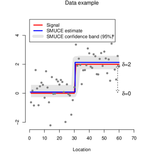
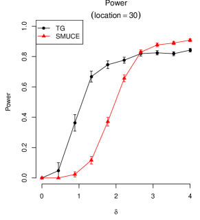
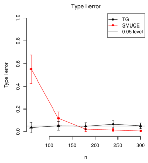
Figure 10: Comparison of p-values from the TG test, and derived from the SMUCE simultaneous confidence band, for testing the same null hypothesis. Data were generated under a problem setup that is the same as that in the top left panel of Figure 8, but with the signal strength $\delta$ varying between 0 and 4. The top left panel of the current figure shows an example with $\delta=2$. In each simulation, the 1d fused lasso path was stopped using the 2-rise BIC rule, and segment test contrasts were formed around the detected changepoints. The middle panel shows power curves, computed over simulations in which the location 30 appeared in the model selected by BIC. These power curves were computed either from the SMUCE band having nominal confidence level 0.95, or the TG test with a type I error control of 0.05. We can see that the latter method has better power for smaller $\delta$, and both perform well for larger $\delta$, with the SMUCE-based method providing slightly more power. The right panel displays the empirical type I error of the two testing methods, which emphasizes that the SMUCE guarantees are only asymptotic, and this method can quite become conservative for large $n$, because in a way simultaneous coverage is a more abitious goal that post-selection coverage.

5.3 Trend filtering example

We examine a problem with $n=40$, and where $\theta\in\mathbb{R}^{40}$ has its first 20 components equal to zero, and its next 20 components exhbiting a linear trend of slope $\delta/20$. Data $y\in\mathbb{R}^{60}$ were generated by adding i.i.d. $\mathcal{N}(0,1)$ noise to $\theta$. We considered the four settings: $\delta=0$ (no signal), $\delta=1$ (weak signal), $\delta=2$ (moderate signal), and $\delta=5$ (strong signal). See the left panel of Figure 11 for an example. We computed the trend filtering path, stopped using the 2-rise BIC rule, and considered the segment test at location 20. The right panel of Figure 11 shows the resulting p-values, restricted to repetitions in which location 20 appeared in the eventual model. We can see that when $\delta=0$, the p-values are uniformly distributed, as we should expect them to be. As $\delta$ increases, we can also see the increase in power, with the jump from $\delta=2$ to $\delta=5$ providing the segment test with nearly full power.

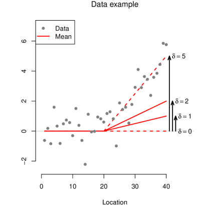
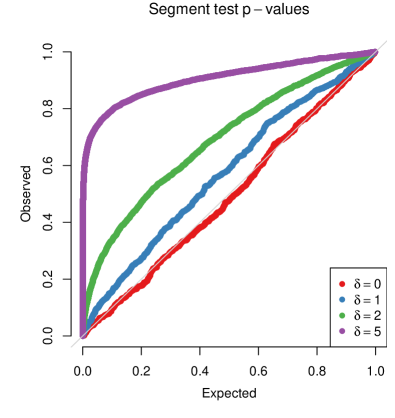
Figure 11: Inferences from the segment test, in a setup with $n=40$ points, and one knot in the underlying piecewise linear mean at location 20, with the change in slope is $\delta/20$. We considered the settings $\delta=0,1,2,5$. The left panel displays an example simulated data set from this setup, for $\delta=5$. The right panel shows QQ plots of segment test p-values at location 20, computed from the trend filtering path, stopped by the 2-rise BIC rule. The p-values were restricted to repetitions in which location 20 appeared in the BIC-selected model. When $\delta=0$, we see uniform p-values, as appropriate; when $\delta=5$, we see nearly full power.

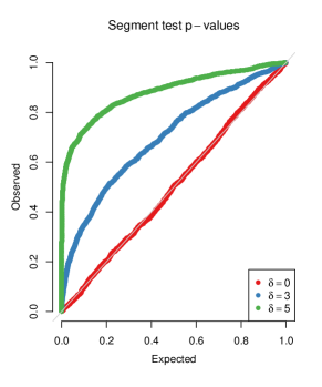
Figure 12: Inferences from the segment test, in a 2d problem setup with $n=100$, and a mean parameter $\theta$ shaped into a piecewise constant $10\times 10$ image. The bottom $5\times 5$ block of the mean is assigned a height of $\delta$, and the rest of its components 0. We considered the settings $\delta=0,3,5$. The left panel visualizes the mean $\theta$, when $\delta=3$; the middle panel shows an example noisy realization $y$, again for $\delta=3$. The right panel shows QQ plots of the segment test, with respect to two fused components appearing in the 2d fused lasso estimate, stopped by the 1-rise BIC stopping rule. When $\delta=3,5$ these p-values are restricted to data instances in which the components being tested are the lower left $5\times 5$ block and its complement; when $\delta=0$, all p-values are shown. The p-values behave as we would expect: uniform for $\delta=0$, and increasing power for $\delta=3,5$.

5.4 2d fused lasso example

We examine a problem setup where the mean $\theta$ is defined over a 2d grid of dimension $10\times 10$ (so that $n=100$), having all components set to zero, except for a $5\times 5$ patch in the lower left corner where all components are equal to $\delta$. Data $y\in\mathbb{R}^{100}$ were generated by adding i.i.d. $\mathcal{N}(0,1)$ noise to $\theta$. We considered the following settings: $\delta=0$ (no signal), $\delta=3$ (medium signal), and $\delta=5$ (strong signal). See the left panel of Figure 12 for a visualization of the mean $\theta$, and the middle panel for example data $y$, both when $\delta=3$.

Over many draws of data from the described simulation setup, we computed the 2d fused lasso solution path, and used the 1-rise BIC stopping rule. For $\delta=3,5$, we retained only the repetitions in which the BIC-chosen 2d fused lasso estimate had exactly two separate fused components—the bottom left $5\times 5$ patch, and its complement—and computed segment test p-values with respect to these two components. For $\delta=0$, we collected the segment test p-values over all repetitions, which were computed with respect to two arbitrary components appearing in the BIC-chosen estimate, in each data instance. The right panel of Figure 12 shows QQ plots for each value of $\delta$ in consideration. When $\delta=0$, we see uniform p-values, as expected; when $\delta=3,5$, we see clear power.

5.5 Regression example

We consider a semi-synthetic stock example, with $n=251$ timepoints, and data $y\in\mathbb{R}^{251}$ simulated from a linear model of log daily returns of 3 real Dow Jones Industrial Average (DJIA) stocks, from the year 2015. Data was obtained from quantmod R package. See the left panel of Figure 13 for a visualization of these stocks (note that what is displayed is not the log daily returns of the stocks, but the raw stock prices themselves).

Denoting the log daily returns as $X_{j}\in\mathbb{R}^{251}$, $j=1,2,3$, our model for the data was

$$y_{t}=\sum_{j=1}^{3}X_{tj}\beta^{*}_{jt}+\epsilon_{jt},\quad\epsilon_{jt}\sim\mathcal{N}(0,\sigma^{2}),\quad\text{i.i.d., for $t=1,\ldots,T$}.$$ (44)

The coefficient vectors $\beta^{*}_{j}\in\mathbb{R}^{251}$, $j=1,2,3$ were taken to be piecewise constant; the first coefficient vector $\beta^{*}_{1}$ had two changepoints at locations 83 and 166, and had constant levels -1, 1, -1 from left to right; the second coefficient vector $\beta^{*}_{2}$ had one changepoint at location 125, switching from levels -1 to 1; the third coefficient vector $\beta^{*}_{3}$ had no changepoints, and was set to have a constant level of 1. We generated data once from the model in (44), with $\sigma=0.002$ (this is a reasonable noise level, as the log daily returns are on a comparable scale). We then computed the fused lasso regression path, where 1d fused lasso penalties were placed on the coefficient vectors for each of the 3 stocks, in order to enforce piecewise constant behavior in the estimates $\hat{\beta}_{j}\in\mathbb{R}^{251}$, $j=1,2,3$. The path was terminated using the 2-rise BIC stopping rule, which gave a final model with 9 changepoints among the coefficient estimates. After post-processing (“decluttering”) changepoints that occurred within 10 locations of each other, we retained 5 changepoints: 2 in the first estimated coefficient vector, 2 in the second, and 1 in the third. Segment test p-values were computed at each of the decluttered changepoints, and 3 changepoints that approximately coincided with true changepoints were found to be significant, while the other 2 were found insignificant. See the right panel of Figure 13. For more details on the fused lasso optimization problem, and the contrasts used to define the segment tests, see Appendix B.

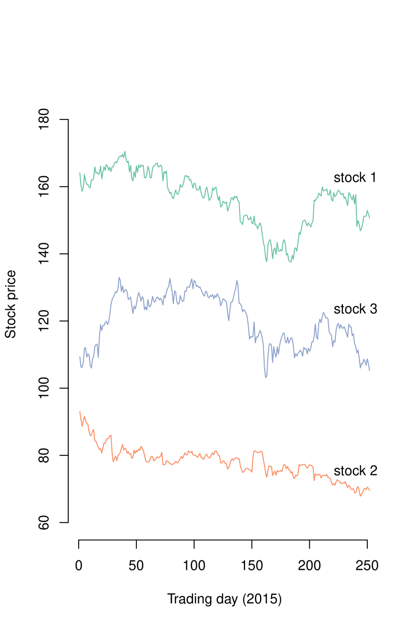
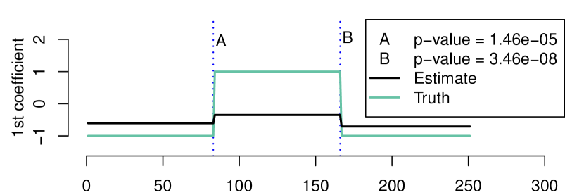
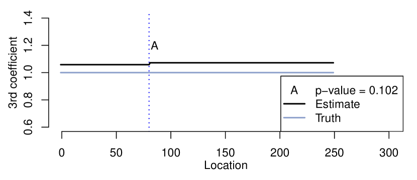
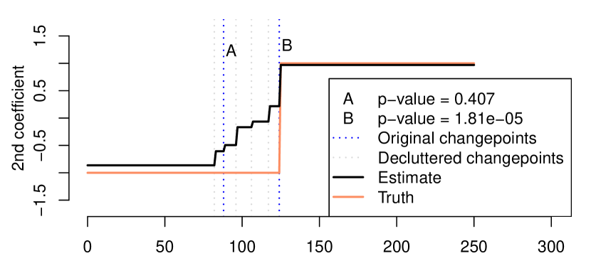
Figure 13: A semi-synthetic stock example, with $n=251$ timepoints or trading days. The left panel shows raw stock prices from three DJIA stocks; response data were generated according to a linear model with the log daily returns of these stocks as predictors, and time-varying coefficients. The true piecewise constant time-varying coefficients are displayed in the right panel. The fused lasso regression path was run, and stopped by the 2-rise BIC rule, delivering the estimated coefficients also displayed in the right panel. After decluttering, segment tests were applied to the detected changepoints and 3 approximately correct locations are deemed significant, with the other 2 spurious detections deemed insignificant.

5.6 Application to CGH data

We examine the use of our fused lasso selective inference tools on a data set of array comparative genomic hybridization (CGH) measurements from two glioblas-toma multiforme (GBM) tumors, from the cghFLasso R package. CGH is a molecular cytogenetic method for determining DNA copy numbers of selected genes in a genome, and array CGH is an improved method which provides higher resolutions measurement. Each CGH measurement is a log ratio of the number of DNA copies of a gene compared to a reference measurement—aberrations give nonzero log ratios. Tibshirani & Wang (2008) considered the sparse 1d fused lasso as a method for identifying regions of DNA copy number aberrations from CGH data, and analyzed the GBM tumor data set as a specific example, with $n=990$ data points.

Using the same GBM tumor data set, we examine the significance of changepoints that appear in the 10th step of the 1d fused lasso path, and separately, changepoints that appear in the 28th step of the sparse 1d fused lasso path (in general, unlike the 1d fused lasso, the sparse 1d fused lasso can add and delete changepoints at each step of the path; the estimate at the 28th step here only had 7 changepoints). These steps were chosen by the 2-rise and 1-rise BIC rules, respectively. The resulting estimates are plotted along with the GBM tumor data, in Figure 14. Displayed below this is a step-sign plot of the sparse 1d fused lasso estimate, serving as example of what might be shown to the scientist to allow him/her to hand-design interesting contrasts to be tested.

Below the plot is a table containing the p-values from segment tests of the changepoints in the two models, i.e., from the 1d fused lasso and sparse 1d fused lasso. The segment test contrasts were post-processed (i.e., “decluttered”) so as to exclude changepoints that occurred within 2 locations of each other—this only affected the locations labeled E and F in the sparse 1d fused lasso model (and as a result, the significance of changepoint at location F was not tested). Commonly detected changepoints occur at locations labeled A, D, E, and G; the segment tests from the 1d fused lasso model yield significant p-values at each of these locations, but those from the sparse 1d fused lasso model only yield a significant p-value at location E. This apparent loss of power with the sparse 1d fused lasso may be due to the larger amount of conditioning involved.

We also compare the above to results from simple changepoint tests carried out using sample splitting. This is possible in a structured problem like ours, where there is a sensible way to split the data (note that in a less structured setting, like a generic graph fused lasso problem, there would be no obvious splitting scheme). We divided the GBM data set into two halves, based on odd and even numbered locations. On the first half, the “estimation set”, we fit the 1d fused lasso path and chose the stopping point using 5-fold cross-validation (CV), where the folds were defined to include every 5th data point in the estimation set. After determining the path step that minimized the CV error, we moved back towards the start of the path (back towards step 1) until a further move would yield a CV error greater than one standard error away from the minimum (this is often called the “one standard error rule”, see, e.g., Chapter 7.10 of Hastie et al. (2009)). This gave a path step of 18, and hence 18 changepoints in the final 1d fused lasso model. Using the second half of the data set, the “testing set”, we then ran simple Z-tests to test for the equality of means between every pair of adjacent segments partitioned by the 18 derived changepoints from the estimation set. For simplicity, in the table in Figure 14, we only show p-values at locations that are comparable to the common locations labeled A, D, E, G from the fused lasso estimation procedures run on the full data set. All are significant.

Lastly, we note that to apply all tests in this subsection, it was necessary to estimate the noise variance $\sigma^{2}$. To do so, we ran 5-fold CV on the full data set, chose the stopping point using the one standard error rule, and estimated $\sigma^{2}$ appropriately based on the residuals. This gave $\hat{\sigma}=0.46$.

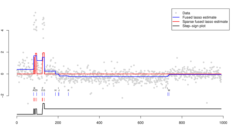
Post-selection
A B C D E F G H I J K L M Test location 81 85 89 96 123 125 133 187 201 204 250 731 737 P-value (non-sparse) 0.00 0.00 0.00 0.00 0.77 0.10 0.47 0.90 0.42 0.58 P-value (sparse) 0.22 0.12 0.89 0.88 0.00 0.13

Sample splitting
Test location 80 96 122 132 P-value (non-sparse) 0.00 0.00 0.00 0.00

Figure 14: A CGH data set of two GBM tumors, from Tibshirani & Wang (2008), with $n=990$ points. The plot displays the 1d fused lasso and sparse 1d fused lasso estimates, in blue and red, respectively, each chosen using an appropriate BIC-based stopping rule (after 2-rises for the non-sparse estimate, and 1-rise for the sparse estimate). The detected changepoints in each of the two models are also labeled. Shown at the bottom of the plot is a step-sign plot of the sparse 1d fused lasso solution. Below the plot are two tables, the first filled with segment test p-values of the changepoints in the 1d fused lasso and sparse 1d fused lasso models. Post-processing of changepoints was applied to rule out changepoints within 2 locations of each other; this only affected the location labeled F in the sparse 1d fused lasso model (hence location F was not tested). The second table shows p-values from a simple sample splitting scheme, where the odd numbered locations were used for fused lasso model fitting and the even numbered locations for changepoint testing. We can see that all three tests mostly agree on the significance of common locations labeled A, D, E, and G, though the sparse 1d fused lasso p-values appear to be under-powered.

6 Discussion

We have extended the post-selection inference framework of Lee et al. (2016); Tibshirani et al. (2016) to the model selection events along the generalized lasso path, as studied by Tibshirani & Taylor (2011). The generalized lasso framework covers a fairly wide range of problem settings, such as the 1d fused lasso, trend filtering, the graph fused lasso, and regression problems in which fused lasso or trend filtering penalties are applied to the coefficients. In this work, we developed a set of tools for conduting formal inferences on components of the adaptively fitted generalized lasso model—these are, e.g., adaptively fitted changepoints in the 1d fused lasso, knots in trend filtering, and clusters in the graph fused lasso. Our methods allow for inferences to be conducted at any fixed step of the generalized lasso solution path, or alternatively, at a step chosen by a rule that tracks AIC or BIC until a given number of rises in the criterion is encountered.

It is worth noting the following important point. In the language of Fithian et al. (2014, 2015), the development of post-selection tests in this paper was done under a “saturated model” for the mean parameter $\theta$—this treats $\theta$ as an arbitrary vector in $\mathbb{R}^{n}$, and the hypotheses being tested are all phrased in terms of certain linear contrasts of the mean parameter begin zero, as in $v^{T}\theta=0$. Fithian et al. (2014, 2015) show how to also conduct tests under the “selected model”—to use the 1d fused lasso as an example, this would model the mean as a vector that is piecewise constant with breaks at the selected changepoints. The techniques developed in Fithian et al. (2015), allow us to perform sequential tests of the selected model—again to use the 1d fused lasso as an example, this would allow us to test, at each step of the 1d fused lasso path, that the mean is piecewise constant in the changepoints detected over all previous steps, and thus a failure to reject would mean that all relevant changepoints have already been found. The selected model tests of Fithian et al. (2015) have the following desirable properties: (i) they do not require the marginal error variance $\sigma^{2}$ to be known; (ii) they often display better power (compared to the tests from this paper) when the selected model is false; (iii) they yield independent p-values across steps in the path for which the selected model is true. The latter property allows us to apply p-value aggregation rules, like the “ForwardStop” rule of Grazier G’Sell et al. (2016), to choose a stopping point in the path, with a guarantee on the FDR. This is an appealing alternative to the AIC- or BIC-based stopping rules described in Section 3.2. The downside of the selected model tests is that they are computationally expensive (compared to those described in this paper), and require sampling (rather than analytic computation, using a truncated Gaussian pivot) to compute p-values. Furthermore, once we use the selected model p-values to choose a stopping point in the path, it is not clear how to carry out valid post-selection tests in the resulting model (due to the corresponding conditioning region being very complicated). Investigation of selected model inference along the generalized lasso path will be the topic of future work.

There are several other possible follow-up ideas for future work. One that we are particularly keen on is the attachment of post-selection inference tools to existing, commonly-used methods for 1d changepoint detection. It is not hard to show that the selection events associated with many such methods—like binary segmentation, wild binary segmentation of Fryzlewicz (2014), and all wavelet thresholding procedures (provided that soft- or hard-thresholding is used)—can be characterized as polyhedral sets in the data $y$. The ideas in this paper can therefore be used to conduct significance tests for the detected changepoints after any number of steps of binary segmentation, wild binary segmentation, or wavelet thresholding, this number of steps either being fixed or chosen by an AIC- or BIC-type rule. Because other 1d changepoint detection methods can often outperform the 1d fused lasso in terms of their accuracy in selected relevant changepoints (wild binary segmentation, specifically, has this property), pairing them with formal tools for inference could have important practical implications.

Appendix A QQ plots for the 1d fused lasso at one-off detections

We consider the same simulation setup as in the top row of Figure 8, where, recall, the sample size was $n=60$ and the mean $\theta\in\mathbb{R}^{60}$ had a single changepoint at location 30. Here we consider the changepoint to have height $\delta=2$, draw data $y\in\mathbb{R}^{60}$ around $\theta$ using i.i.d. $\mathcal{N}(0,1)$ errors, and retain instances in which 1 step of the fused lasso path detects a changepoint at location 29 or 31, i.e., off by one from the true location 30. Figure 15 (right panel) shows QQ plots for the spike and segment tests, applied to test the significance of the detected changepoint, in these instances. We can see that the spike test p-values are uniformly distributed, which is appropriate, because when the detected changepoint is off by one, the spike test null hypothesis is true. The segment test, on the other hand, delivers very small p-values, giving power against its own null hypothesis, which is false in the case of a one-off detection.

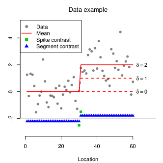
Figure 15: The left panel is copied from Figure 8 in the main text, and shows an example data set with $n=60$ and a piecewise constant mean $\theta$ with one jump at location 30. The right panel shows QQ plots from the spike and segment tests run at the detected changepoint from the 1-step fused lasso, over data instances in which the detected changepoint occurred at location 29 or 30, i.e., off by one from the true location 30. We can see that the spike test p-values are uniform, and the segment test p-values are highly sub-uniform.

Appendix B Regression example details

Recall the notation of Section 5.5, where $X_{j}\in\mathbb{R}^{251}$, $j=1,2,3$ denote the log daily returns of 3 real DJIA stocks, and $\beta^{*}_{j}\in\mathbb{R}^{251}$, $j=1,2,3$ were synthetic piecewise constant coefficient vectors. Denote by $\theta\in\mathbb{R}^{251}$ the mean vector, having components

$$\theta_{t}=\sum_{j=1}^{3}X_{tj}\beta^{*}_{jt},\quad t=1,\ldots,251.$$

Denote by $X\in\mathbb{R}^{251\times 753}$ the predictor matrix

$$X=\left[\begin{array}[]{ccc}\mathrm{diag}(X_{1})&\mathrm{diag}(X_{2})&\mathrm{diag}(X_{3})\end{array}\right],$$

where $\mathrm{diag}(X_{j})\in\mathbb{R}^{251\times 251}$ is the diagonal matrix in the entries $X_{j1},\ldots,X_{j,253}$, $j=1,2,3$. Also, let $\beta^{*}=(\beta_{1}^{*},\beta_{2}^{*},\beta_{3}^{*})\in\mathbb{R}^{753}$. Then, in this abbreviated notation, the mean is simply $\theta=X\beta^{*}$, and data is generated according to the model regression model $y\sim N(\theta,\sigma^{2}I)$.

Optimization problem.

The fused lasso regression problem that we consider is

$$\hat{\beta}=\mathop{\mathrm{argmin}}_{\beta\in\mathbb{R}^{751}}\;\frac{1}{2}\|y-X\beta\|_{2}^{2}+\lambda\|D\beta\|_{1}+\rho\|\beta\|_{2}^{2},$$ (45)

where $X\in\mathbb{R}^{251\times 753}$ is as defined above, and using a block decomposition $\beta=(\beta_{1},\beta_{2},\beta_{3})\in\mathbb{R}^{751}$, with each $\beta_{j}\in\mathbb{R}^{251}$, we may write the penalty matrix $D\in\mathbb{R}^{750\times 251}$ as

$$D=\left[\begin{array}[]{c}D^{(1)}\\ D^{(1)}\\ D^{(1)}\end{array}\right],\quad\text{where}\quad D^{(1)}=\left[\begin{array}[]{ccccc}-1&1&0&\ldots&0\\ 0&-1&1&\ldots&0\\ \vdots&&\ddots&\ddots&\\ 0&0&\ldots&-1&1\end{array}\right]\in\mathbb{R}^{250\times 251},$$

so that $\|D\beta\|_{1}=\sum_{j=}^{3}\|D^{(1)}\beta_{j}\|_{1}$. Note that small ridge penalty has been added to the criterion in (45) (i.e., $\rho>0$ is taken to be a small fixed constant), making the problem strictly convex, thus ensuring it has a unique solution, and also ensuring that we can run the dual path algorithm of Tibshirani & Taylor (2011). Of course, the blocks of the solution $\hat{\beta}=(\hat{\beta}_{1},\hat{\beta}_{2},\hat{\beta}_{3})$ in (45) serve as estimates of the underlying coefficient vectors $\beta_{1}^{*},\beta_{2}^{*},\beta_{3}^{*}$.

Segment test contrasts.

Having specified the details of the generalized lasso regression problem solved in Section 5.5, it remains to specify the contrasts that were used to form the segment tests. Let $\mathcal{B}\subseteq\{1,\ldots,753\}$ be the indices of changepoints in the solution $\hat{\beta}$, assumed to be in sorted order. We can decompose $\mathcal{B}=\mathcal{B}_{1}\cup(251+\mathcal{B}_{2})\cup(452+\mathcal{B}_{3})$, where each $\mathcal{B}_{j}\subseteq\{1,\ldots,251\}$, $j=1,2,3$. Write $X_{\mathcal{B}}\in\mathbb{R}^{251\times{|\mathcal{B}|+3}}$ for the “effective” design matrix when changepoints occur in $\mathcal{B}$, whose columns are defined by splitting each $X_{j}$ into segments that correspond to breakpoints in $\mathcal{B}_{j}$, and collecting these across $j=1,2,3$. For example, if $\mathcal{B}_{1}=\{60,125\}$, then $X_{1}$ gets split into $|\mathcal{B}_{1}|+2=3$ columns:

$$\left[\begin{array}[]{c}X_{j1}\\ \vdots\\ X_{j,60}\\ 0\\ \vdots\\ 0\\ 0\\ \vdots\\ 0\end{array}\right],\;\;\left[\begin{array}[]{c}0\\ \vdots\\ 0\\ X_{j,61}\\ \vdots\\ X_{j,125}\\ 0\\ \vdots\\ 0\end{array}\right],\;\;\left[\begin{array}[]{c}0\\ \vdots\\ 0\\ 0\\ \vdots\\ 0\\ X_{j,126}\\ \vdots\\ X_{j,251}\end{array}\right].$$

For each detected changepoint $I_{j}\in\mathcal{B}$, we now define a segment test contrast vector by

$$v_{\mathrm{seg}}=s_{I_{j}}(X_{\mathcal{B}}^{+})^{T}(0,\ldots,0,\underset{\underset{r_{I_{j}}}{\uparrow}}{-1},\underset{\underset{r_{I_{j}}+1}{\uparrow}}{1},0,\ldots,0),$$ (46)

where $s_{I_{j}}$ is the observed sign of the difference between coordinates $I_{j}$ and $I_{j}+1$ of the fused lasso solution $\hat{\beta}$, and $r_{I_{J}}$ is the rank of $I_{j}$ in $\mathcal{B}$. Then the TG statistic in (12), with $v=v_{\mathrm{seg}}$, tests

$$H_{0}:(0,\ldots,0,\underset{\underset{r_{I_{j}}}{\uparrow}}{-1},\underset{\underset{r_{I_{j}}+1}{\uparrow}}{1},0,\ldots,0)^{T}X_{\mathcal{B}}^{+}\theta=0\quad\text{versus}\quad H_{1}:s_{I_{J}}(0,\ldots,0,\underset{\underset{r_{I_{j}}}{\uparrow}}{-1},\underset{\underset{r_{I_{j}}+1}{\uparrow}}{1},0,\ldots,0)^{T}X_{\mathcal{B}}^{+}\theta>0.$$ (47)

In words, this tests whether the best linear model fit to the mean $\theta$, using the effective design $X_{\mathcal{B}}$, yields coefficents that match on either side of the changepoint $I_{j}$. The alternative hypothesis is that they are different and the sign of the difference is the same as the sign in the fused lasso solution.

Alternative motivation for the contrasts.

An alternative motivation for the above definition of contrast at a changepoint $I_{j}\in\mathcal{B}$ stems from consideration of the hypotheses

$$H_{0}:\theta\in\mathrm{col}(X_{\mathcal{B}\setminus\{I_{j}\}})\quad\text{versus}\quad H_{1}:\theta\in\mathrm{col}(X_{\mathcal{B}}).$$

When $\mathcal{B}$ is considered to be fixed (and hence so are these hypotheses), the corresponding likelihood ratio test is is $v_{\mathrm{lik}}^{T}y$, where $v_{\mathrm{lik}}$ is a unit vector that spans the rank 1 subspace $\mathrm{col}(X_{\mathcal{B}\setminus\{I_{j}\}})^{\perp}\mathrm{col}(X_{\mathcal{B}})$, i.e.,

$$v_{\mathrm{lik}}v_{\mathrm{lik}}^{T}=P_{\mathrm{col}(X_{\mathcal{B}})}-P_{\mathrm{col}(X_{\mathcal{B}\setminus\{I_{j}\}})}.$$ (48)

We now prove that indeed, $v_{\mathrm{lik}}$ in (48) and $v_{\mathrm{seg}}$ in (46) are equal up to normalization. Abbreviate

$$w=(0,\ldots,0,\underset{\underset{r_{I_{j}}}{\uparrow}}{-1},\underset{\underset{r_{I_{j}}+1}{\uparrow}}{1},0,\ldots,0),$$

and $M=\mathcal{B}$, $m=X_{\mathcal{B}\setminus\{I_{j}\}}$. It suffices to show that

$$(X_{M}^{+})^{T}ww^{T}X_{M}^{+}\;\propto\;X_{M}X_{M}^{+}-X_{m}X_{m}^{+}.$$

To verify the above, multiply from the left by $X_{M}^{+}$ and from the right by $X_{M}$, and assuming with a loss of generality that $X_{M}$ has full column rank, we get

$$ww^{T} \;\propto\;X_{M}^{T}X_{M}-X_{M}^{T}X_{m}X_{m}^{+}X_{M}$$

$$=X_{M}^{T}(I-X_{m}X_{m}^{+})X_{M}$$

$$=X_{M}^{T}P_{\mathrm{col}(X_{m})}^{\perp}X_{M}$$

$$=X_{M}^{T}P_{\mathrm{col}(X_{m})}^{\perp}P_{\mathrm{col}(X_{m})}^{\perp}X_{M}.$$

But it is easy to see that $X_{M}^{T}P_{\mathrm{col}(X_{m})}^{\perp}P_{\mathrm{col}(X_{m})}^{\perp}X_{M}$ is proportional to $ww^{T}$, because if $a$ is any vector that has identical entries across coordinates $r_{I_{j}}$ and $r_{I_{j}}+1$, then

$$P_{\mathrm{col}(X_{m})}^{\perp}X_{M}a=P_{\mathrm{col}(X_{m})}^{\perp}X_{m}a^{\prime}=0,$$

where $a^{\prime}$ is simply $a$ with its $(r_{I_{j}})$th coordinate removed. This completes the proof.

References

- (1)
- Arnold & Tibshirani (2016) Arnold, T. & Tibshirani, R. J. (2016), ‘Efficient implementations of the generalized lasso dual path algorithm’, Journal of Computational and Graphical Statistics 25(1), 1–27.
- Bai (1999) Bai, J. (1999), ‘Likelihood ratio tests for multiple structural changes’, Journal of Econometrics 91(2), 299–323.
- Berk et al. (2013) Berk, R., Brown, L., Buja, A., Zhang, K. & Zhao, L. (2013), ‘Valid post-selection inference’, Annals of Statistics 41(2), 802–837.
- Brodsky & Darkhovski (1993) Brodsky, B. & Darkhovski, B. (1993), Nonparametric Methods in Change-Point Problems, Springer, Netherlands.
- Chambolle & Darbon (2009) Chambolle, A. & Darbon, J. (2009), ‘On total variation minimization and surface evolution using parametric maximum flows’, International Journal of Computer Vision 84, 288–307.
- Chen & Chen (2008) Chen, J. & Chen, Z. (2008), ‘Extended Bayesian information criteria for model selection with large model spaces’, Biometrika 95(3), 759–771.
- Chen & Gupta (2000) Chen, J. & Gupta, A. (2000), Parametric Statistical Change Point Analysis, Birkhauser, Basel.
- Choi et al. (2014) Choi, Y., Taylor, J. & Tibshirani, R. (2014), Selecting the number of principal components: estimation of the true rank of a noisy matrix. arXiv: 1410.8260.
- Eckley et al. (2011) Eckley, I., Fearnhead, P. & Killick, R. (2011), Analysis of changepoint models, in D. Barber, T. Cemgil & S. Chiappa, eds, ‘Bayesian Time Series Models’, Cambridge University Press, Cambridge, chapter 10, pp. 205–224.
- Fithian et al. (2014) Fithian, W., Sun, D. & Taylor, J. (2014), Optimal inference after model selection. arXv: 1410.2597.
- Fithian et al. (2015) Fithian, W., Taylor, J., Tibshirani, R. & Tibshirani, R. J. (2015), Selective sequential model selection. arXiv: 1512.02565.
- Frick et al. (2014) Frick, K., Munk, A. & Sieling, H. (2014), ‘Multiscale change point inference’, Journal of the Royal Statistical Society. Series B: Statistical Methodology 76(3), 495–580.
- Friedman et al. (2007) Friedman, J., Hastie, T., Hoefling, H. & Tibshirani, R. (2007), ‘Pathwise coordinate optimization’, Annals of Applied Statistics 1(2), 302–332.
- Fryzlewicz (2014) Fryzlewicz, P. (2014), ‘Wild binary segmentation for multiple change-point detection’, Annals of Statistics 42(6), 2243–2281.
- Grazier G’Sell et al. (2016) Grazier G’Sell, M., Wager, S., Chouldechova, A. & Tibshirani, R. (2016), ‘Sequential selection procedures and false discovery rate control’, Journal of the Royal Statistical Society: Series B 78(2), 423–444.
- Hastie et al. (2009) Hastie, T., Tibshirani, R. & Friedman, J. (2009), The Elements of Statistical Learning; Data Mining, Inference and Prediction, Springer, New York. Second edition.
- Hinkley (1970) Hinkley, D. (1970), ‘Inference about the change-point in a sequence of random variables’, Biometrika 57(1), 1–17.
- Hoefling (2010) Hoefling, H. (2010), ‘A path algorithm for the fused lasso signal approximator’, Journal of Computational and Graphical Statistics 19(4), 984–1006.
- Horvath & Rice (2014) Horvath, L. & Rice, G. (2014), ‘Extensions of some classical methods in change point analysis’, TEST 23(2), 219–255.
- Jandhyala et al. (2013) Jandhyala, V., Fotopoulos, S., Macneill, I. & Liu, P. (2013), ‘Inference for single and multiple change-points in time series’, Journal of Time Series Analysis 34(4), 423–446.
- Kim et al. (2009) Kim, S.-J., Koh, K., Boyd, S. & Gorinevsky, D. (2009), ‘ trend filtering’, SIAM Review 51(2), 339–360.
- Lee et al. (2016) Lee, J., Sun, D., Sun, Y. & Taylor, J. (2016), ‘Exact post-selection inference with application to the lasso’, Annals of Statistics . To appear.
- Lee & Taylor (2014) Lee, J. & Taylor, J. (2014), ‘Exact post model selection inference for marginal screening’, Advances in Neural Information Processing Systems 27.
- Leeb & Potscher (2003) Leeb, H. & Potscher, B. (2003), ‘The finite-sample distribution of post-model-selection estimators and uniform versus nonuniform approximations’, Econometric Theory 19(1), 100–142.
- Leeb & Potscher (2006) Leeb, H. & Potscher, B. (2006), ‘Can one estimate the conditional distribution of post-model-selection estimators?’, Annals of Statistics 34(5), 2554–2591.
- Leeb & Potscher (2008) Leeb, H. & Potscher, B. (2008), ‘Can one estimate the unconditional distribution of post-model-selection estimators?’, Econometric Theory 24(2), 338–376.
- Lockhart et al. (2014) Lockhart, R., Taylor, J., Tibshirani, R. J. & Tibshirani, R. (2014), ‘A significance test for the lasso’, Annals of Statistics 42(2), 413–468.
- Loftus & Taylor (2014) Loftus, J. & Taylor, J. (2014), A significance test for forward stepwise model selection. arXiv: 1405.3920.
- Reid et al. (2014) Reid, S., Taylor, J. & Tibshirani, R. (2014), Post-selection point and interval estimation of signal sizes in Gaussian samples. arXiv: 1405.3340.
- Rudin et al. (1992) Rudin, L. I., Osher, S. & Faterni, E. (1992), ‘Nonlinear total variation based noise removal algorithms’, Physica D: Nonlinear Phenomena 60, 259–268.
- Sharpnack et al. (2012) Sharpnack, J., Rinaldo, A. & Singh, A. (2012), ‘Sparsistency of the edge lasso over graphs’, Proceedings of the International Conference on Artificial Intelligence and Statistics 15, 1028–1036.
- Steidl et al. (2006) Steidl, G., Didas, S. & Neumann, J. (2006), ‘Splines in higher order TV regularization’, International Journal of Computer Vision 70(3), 214–255.
- Tian & Taylor (2015a) Tian, X. & Taylor, J. (2015a), Asymptotics of selective inference. arXiv: 1501.03588.
- Tian & Taylor (2015b) Tian, X. & Taylor, J. (2015b), Selective inference with a randomized response. arXiv: 1507.06739.
- Tibshirani (2014) Tibshirani, R. J. (2014), ‘Adaptive piecewise polynomial estimation via trend filtering’, Annals of Statistics 42(1), 285–323.
- Tibshirani et al. (2015) Tibshirani, R. J., Rinaldo, A., Tibshirani, R. & Wasserman, L. (2015), Uniform asymptotic inference and the bootstrap after model selection. arXiv: 1506.06266.
- Tibshirani & Taylor (2011) Tibshirani, R. J. & Taylor, J. (2011), ‘The solution path of the generalized lasso’, Annals of Statistics 39(3), 1335–1371.
- Tibshirani & Taylor (2012) Tibshirani, R. J. & Taylor, J. (2012), ‘Degrees of freedom in lasso problems’, Annals of Statistics 40(2), 1198–1232.
- Tibshirani et al. (2016) Tibshirani, R. J., Taylor, J., Lockhart, R., & Tibshirani, R. (2016), ‘Exact post-selection inference for sequential regression procedures’, Journal of the American Statistical Association . To appear.
- Tibshirani et al. (2005) Tibshirani, R., Saunders, M., Rosset, S., Zhu, J. & Knight, K. (2005), ‘Sparsity and smoothness via the fused lasso’, Journal of the Royal Statistical Society: Series B 67(1), 91–108.
-
Tibshirani & Wang (2008)
Tibshirani, R. & Wang, P. (2008),
‘Spatial smoothing and hot spot detection for CGH data using the fused
lasso’, Biostatistics 9(1), 18–29.
http://www.ncbi.nlm.nih.gov/pubmed/17513312 - Wang et al. (2016) Wang, Y.-X., Sharpnack, J., Smola, A. & Tibshirani, R. J. (2016), ‘Trend filtering on graphs’. To appear in Journal of Machine Learning Research.
- Worsley (1986) Worsley, K. J. (1986), ‘Confidence-regions and tests for a change-point in a sequence of exponential family random-variables’, Biometrika 73(1), 91–104.