A Critical Value Function Approach, with an Application to Persistent Time-Series

Abstract

Researchers often rely on the t-statistic to make inference on parameters in statistical models. It is common practice to obtain critical values by simulation techniques. This paper proposes a novel numerical method to obtain an approximately similar test. This test rejects the null hypothesis when the test statistic is larger than a critical value function (CVF) of the data. We illustrate this procedure when regressors are highly persistent, a case in which commonly-used simulation methods encounter difficulties controlling size uniformly. Our approach works satisfactorily, controls size, and yields a test which outperforms the two other known similar tests.

, and

1 Introduction

The exact distribution of a test statistic is often unknown to the researcher. If the statistic is asymptotically pivotal, the quantile based on the limiting distribution is commonly used as a critical value. Simulation methods aim to find approximations to such a quantile, including the Quenouille-Tukey jackknife, the bootstrap method of Efron [8], and the subsampling approach of Politis and Romano [16]. These methods are valid for a variety of models, as proved by Bickel and Freedman [4], Politis et al. [17], and Romano and Shaikh [18].

For some testing problems, however, the distribution of a statistic can actually be sensitive to the unknown probability distribution. This dependence can be related to the curvature of the model, in the sense of Efron [6, 7], not vanishing asymptotically. This curvature creates difficulty in drawing inference on parameters of interest. Usual tests may not control size uniformly and confidence regions do not necessarily cover the true parameter at the nominal level. As standard simulation methods may not circumvent the sensitivity to unknown parameters, there is a need to develop methods that take this dependence into consideration.

The goal of this paper is to directly tackle the core of the problem, adjusting for the sensitivity of the test statistic to nuisance parameters. In practice, our method entails replacing a critical value number by a critical value function (CVF) of the data. The CVF is a linear combination of density ratios under the null distribution. The weight choice in this combination is at the discretion of the researcher. We focus here on combinations that yield tests which are approximately similar. These weights can be found by linear programming (LP).

We illustrate the CVF procedure with a simple but important model in which the regressor may be integrated. Jeganathan [11, 12] shows that the limit of experiments is Locally Asymptotically Brownian Functional (LABF). The usual test statistics are no longer asymptotically pivotal and the theory of optimal tests based on Locally Asymptotically Mixed Normal (LAMN) experiments is no longer applicable. The bootstrap and subsampling may not provide uniform control in size and confidence levels, as discussed by Basawa et al. [2] and Politis and Romano [16], among others. The similar t-test based on the CVF has null rejection probabilities close to the nominal level regardless of the value of the autoregressive parameter. While this paper does not focus on obtaining optimal procedures, the proposed similar t-test does have good power. It has correct size and outperforms the two other tests that are known to be similar: the $L_{2}$ test of Wright [21] and the uniformly most powerful conditionally unbiased (UMPCU) test of Jansson and Moreira [10].

This paper is organized as follows. Section 2 introduces the CVF approach and shows how to find tests which are approximately similar in finite samples. Section 3 presents the predictive regressor model and obtains approximations that are asymptotically valid whether the disturbances are normal or not. Section 4 provides numerical simulations to compare the similar t-test with existing procedures in terms of size and power. Section 5 concludes. Appendix A provides a bound based on a discrepancy error useful to implement the CVF. Appendix B contains the proofs to the theory underlying the CVF. The supplement presents additional numerical results and remaining proofs.

2 Inference Based on the t-Statistic

Commonly used tests for $H_{0}:\beta\leq\beta_{0}$ against $H_{1}:\beta>\beta_{0}$ reject the null hypothesis when some statistic $\psi$ is larger than a critical value $\kappa_{\alpha}$ (we omit here the dependence of the statistic $\psi$ on the data $R$ for convenience). The test is said to have size $\alpha$ when the null rejection probability is no larger than $\alpha$ for any value of the nuisance parameter $\gamma$:

$$\sup_{\beta\leq\beta_{0},\gamma\in\Gamma}P_{\beta,\gamma}\left(\psi>\kappa_{\alpha}\right)=\alpha.$$ (2.1)

Finding the critical value $\kappa_{\alpha}$ that satisfies (2.1) is a difficult task as the null distribution of the statistic $\psi$ is unknown. In practice, the choice of $\kappa_{\alpha}$ is based on the limiting distribution of $\psi$ for a large sample size $T$. If $\psi$ is asymptotically pivotal, the null rejection probability at $\beta_{0}$ is approximately $\alpha$:

$$\lim_{T\rightarrow\infty}P_{\beta_{0},\gamma}\left(\psi>\kappa_{\alpha}\right)=\alpha.$$ (2.2)

The t-test rejects the null hypothesis when the t-statistic is larger than a critical value:

$$\psi\left(r\right)>\kappa_{\alpha}.$$

Simulation methods aim to find approximations to the critical value $\kappa_{\alpha}$. In most cases, the limit of experiments is locally asymptotically mixed normal (LAMN) and the t-statistic is asymptotically normal. Hence, numerical methods are usually not too sensitive to the true unknown nuisance parameter. This critical value number can be simulated using sample draws. The bootstrap approach works if the asymptotic critical value does not depend on $\gamma$ within the correct neighborhood around the true parameter value. In some problems, however, the curvature does not vanish asymptotically. For example, take the case in which the regressors are persistent. Cavanagh et al. [5] show that several standard methods fail to control size uniformly. This failure is due to the model curvature not vanishing when the series is nearly integrated. In particular, the asymptotic quantile of the t-statistic does depend on the nuisance parameters when the autoregressive coefficient $\gamma$ is near one.

2.1 The Critical Value Function

We propose a new method to find a test based on the t-statistic which controls size uniformly. We focus on finding approximately similar tests where the null rejection probability is close to $\alpha$. The approach developed here also holds if we instead want to find tests with correct size (in a uniform sense) in which the null rejection probability is no larger than $\alpha$.

Our approach takes into consideration the dependence of the null rejection probability on $\gamma\in\Gamma$ by means of a critical value function. The proposed test rejects the null hypothesis when

$$\psi\left(r\right)>\kappa_{\Gamma_{n},\alpha}(r),$$ (2.3)

where $\kappa_{\Gamma_{n},\alpha}$ is the critical value function so that the test is similar at $\Gamma_{n}=\left\{\gamma_{1},...,\gamma_{n}\right\}$, a set containing $n$ values of the nuisance parameter $\gamma$. We choose

$$\kappa_{\Gamma_{n},\alpha}(r)=\sum_{i=1}^{n}k_{i}\frac{f_{\beta_{0},\gamma_{i}}(r)}{f_{\nu}\left(r\right)},$$ (2.4)

where $k=\left(k_{1},k_{2},...,k_{n}\right)$ is a vector of dimension $n$ and $f_{\nu}\left(r\right)$ is a density function. By a standard separation theorem (e.g., [15]), there exist scalars $k_{1},k_{2},...,k_{n}$ so that

$$P_{\beta_{0},\gamma_{i}}\left(\psi\left(R\right)>\kappa_{\Gamma_{n},\alpha}(R)\right)=\alpha,$$ (2.5)

for $i=1,...,n$. Under some regularity conditions, the scalars $k_{1},k_{2},...,k_{n}$ are unique.

The critical value function $\kappa_{\Gamma_{n},\alpha}(r)$ guarantees that the null rejection probability equals $\alpha$ for $\gamma\in\Gamma_{n}$. With enough discretization, we can ensure that the null rejection probability does not differ from $\alpha$ by more than a discrepancy error $\varepsilon$.

Theorem 1.

Assume that $f_{\beta_{0},\gamma}\left(r\right)$ is continuous in $\gamma$ a.e. in $r$. Consider an array $\gamma_{i,n}$ so that $\sup_{\gamma\in\Gamma}\min_{\gamma_{i,n}\in\Gamma_{n}}\left|\gamma-\gamma_{i,n}\right|\rightarrow 0$ as $n\rightarrow\infty$. Let $\phi_{\Gamma_{n},\alpha}\left(r\right)$ be the test which rejects the null if

$$\psi\left(r\right)>\kappa_{\Gamma_{n},\alpha}(r),$$

where $\Gamma_{n}=\left\{\gamma_{1,n},...,\gamma_{n,n}\right\}$. Then, for any $\epsilon>0$, there exists an $n$ large enough so that

$$\left|E_{\beta_{0},\gamma}\phi_{\Gamma_{n},\alpha}\left(r\right)-\alpha\right|\leq\epsilon,$$

for any value of $\gamma\in\Gamma$.

By Theorem 1, the size is controlled uniformly if the discretization is fine enough. In practice, we can find the set $\Gamma_{n}$ through an iterative algorithm. We can start by choosing two endpoints in the boundary of an interval of interest for $\gamma$. The critical value function ensures that the null rejection probability for those two points is exactly $\alpha$, but not for the other points in that interval. We can proceed by computing the null rejection probabilities for these other points, either analytically or numerically. If at least one of them differs from $\alpha$ by more than a discrepancy error, we include the point whose discrepancy is the largest in the next iteration and start the algorithm all over again. This approach will be discussed in our numerical example in Section 4, where we use Monte Carlo simulations to estimate the null rejection probabilities.

2.2 The Baseline Density Function

By Le Cam’s Third Lemma, the critical value function collapses to a constant if the statistic is asymptotically pivotal and $f_{\nu}\left(r\right)$ is a mixture of densities when $\beta=\beta_{0}$. Hence, we focus on

$$f_{\nu}\left(r\right)=\int f_{\beta_{0},\gamma}\left(r\right)d\nu\left(\gamma\right)\text{,}$$

where $\nu$ is a probability measure which weights different values of $\gamma$.

One example is a weight, $\nu^{\ast}$, which assigns the same mass $1/n$ on a finite number of points $\gamma_{1}<\gamma_{2}<...<\gamma_{n}$:

$$\nu^{\ast}\left(d\gamma\right)=\left\{\begin{array}[]{cc}\frac{1}{n}&\text{if }\gamma=\gamma_{i}\\ 0&\text{otherwise}\end{array}\right..$$

The test then rejects the null hypothesis when

$$\psi\left(r\right)>\frac{\sum_{i=1}^{n}k_{i}f_{\beta_{0},\gamma_{i}}(r)}{n^{-1}\sum_{j=1}^{n}f_{\beta_{0},\gamma_{j}}(r)}.$$

A second probability measure, $\nu^{\dagger}$, assigns all mass on a point $\overline{\gamma}$:

$$\nu^{\dagger}\left(d\gamma\right)=\left\{\begin{array}[]{cc}1&\text{if }\gamma=\overline{\gamma}\\ 0&\text{otherwise}\end{array}\right..$$

The test rejects the null when

$$\psi\left(r\right)>\sum_{i=1}^{n}k_{i}\frac{f_{\beta_{0},\gamma_{i}}(r)}{f_{\beta_{0},\overline{\gamma}}(r)}.$$

The choice of $\overline{\gamma}$ for the baseline density $f_{\nu^{\dagger}}\left(r\right)$ can be motivated by those points for which the limit of experiments is not LAMN. In our leading example in which the regressor is persistent, it may be natural to set the autoregressive parameter $\overline{\gamma}$ equal to one. In practice, however, we recommend using the density average $f_{\nu^{\ast}}\left(r\right)$. By choosing the baseline density as a simple average of the densities $f_{\beta_{0},\gamma_{i}}(r)$, the CVF is bounded and appears to have better numerical performance for other null rejection probabilities beyond $\Gamma=\left\{\gamma_{1},...,\gamma_{n}\right\}$.

2.3 Linear Programming

We can find the multipliers $k_{l}$, $l=1,...,n$, using a linear programming approach. The method is simple and requires a sample drawn from only one probability law. Let $R^{\left(j\right)}$, $j=1,...,J$, be i.i.d. random variables with positive density $f_{\nu^{\ast}}\left(r\right)$.

Consider the maximization problem

$$\max_{0\leq\phi(R^{\left(j\right)})\leq 1}\text{ }\frac{1}{J}\sum_{j=1}^{J}\phi(R^{\left(j\right)})\frac{\psi(R^{\left(j\right)}).f_{\nu}(R^{\left(j\right)})}{f_{\nu^{\ast}}(R^{\left(j\right)})}$$ (2.6)

$$\text{s.t. \ }\frac{1}{J}\sum_{j=1}^{J}\phi(R^{\left(j\right)})\frac{f_{\beta_{0},\gamma_{l}}(R^{\left(j\right)})}{f_{\nu^{\ast}}(R^{\left(j\right)})}=\alpha\text{, }l=1,...,n\text{.}$$

The solution to this problem is given by the test in (2.3) which approximately satisfies the boundary constraints given in (2.5).

We can rewrite the maximization problem as a standard (primal) linear programming problem:

$$\max_{m_{J}\in\left[0,1\right]^{J}}\text{ }d^{\prime}m_{J}$$ (2.7)

$$\text{s.t. \ }Am_{J}=\alpha.1_{n},$$

where $d=\left(\frac{\psi(R^{\left(1\right)}).f_{\nu}(R^{\left(1\right)})}{f_{\nu^{\ast}}(R^{\left(1\right)})},...,\frac{\psi(R^{\left(J\right)}).f_{\nu}(R^{\left(J\right)})}{f_{\nu^{\ast}}(R^{\left(J\right)})}\right)^{\prime}$ and $m_{J}=(\phi(R^{\left(1\right)}),...,\phi(R^{\left(J\right)}))^{\prime}$ are vectors in $\mathbb{R}^{J}$, the $\left(l,j\right)$-entry of the $n\times J$ matrix $A$ is $f_{\beta_{0},\gamma_{l}}(R^{\left(j\right)})/f_{\nu^{\ast}}(R^{\left(j\right)})$, and $1_{n}$ is an $n$-dimensional vector with all coordinates equal to one. The dual program

$$\min_{k_{J}\in\mathbb{R}^{n}}\text{ }1_{n}^{\prime}k_{J}$$ (2.8)

$$\text{s.t. \ }A^{\prime}k_{J}=d$$

yields an approximation to the vector $k$ associated to the critical value function given in (2.4).

The approximation $k_{J}$ to the unknown vector $k$ satisfying (2.5) may, of course, be a poor one. This numerical difficulty can be circumvented if the LLN holds uniformly as $J\rightarrow\infty$ for the sample averages present in the maximization problem given by (2.6). Showing uniform convergence is essentially equivalent to proving that the functions, appearing in the objective function and the boundary constraints of (2.6), belong to the Glivenko-Cantelli class, as defined in van der Vaart [20, p. 145]. A sufficient condition for uniform convergence is that the set $\Gamma$ is compact, the functions $f_{\beta_{0},\gamma}(r)/f_{\nu^{\ast}}(r)$ are continuous in $\gamma$ for every $r$, and $\psi(r)$ is integrable.

3 Application: Persistent Regressors

Consider a simple model with persistent regressors. There is a stochastic equation

$$y_{t}=\mu_{y}+\beta x_{t-1}+\epsilon_{t}^{y},$$

where the variable $y_{t}$ and the regressor $x_{t}$ are observed, and $\epsilon_{t}^{y}$ is a disturbance variable, $t=1,...,T$. This equation is part of a larger model where the regressor can be correlated with the unknown disturbance. More specifically, we have

$$x_{t}=\gamma x_{t-1}+\epsilon_{t}^{x},$$

where $x_{0}=0$ and the disturbance $\epsilon_{t}^{x}$ is unobserved and possibly correlated with $\epsilon_{t}^{y}$. We assume that $\epsilon_{t}=\left(\epsilon_{t}^{y},\epsilon_{t}^{x}\right)\overset{iid}{\sim}N\left(0,\Sigma\right)$ where

$$\Sigma=\left[\begin{array}[]{cc}\sigma_{yy}&\sigma_{xy}\\ \sigma_{xy}&\sigma_{xx}\end{array}\right]$$

is a positive definite matrix. The theoretical results carry out asymptotically whether $\Sigma$ is known or not. For simplicity, we assume for now that $\Sigma$ is known.

Our goal is to assess the predictive power of the past value of $x_{t}$ on the current value of $y_{t}$. For example, a variable observed at time $t-1$ can be used to forecast another in period $t$. The null hypothesis is $H_{0}:\beta\leq 0$ and the alternative is $H_{1}:\beta>0$.

For example, consider the t-statistic

$$\psi=\frac{\widehat{\beta}-\beta_{0}}{\sigma_{yy}^{1/2}\left[\sum_{t=1}^{T}\left(x_{t-1}^{\mu}\right)^{2}\right]^{-1/2}},$$ (3.9)

where $\widehat{\beta}=\sum_{t=1}^{T}x_{t-1}^{\mu}y_{t}/\sum_{t=1}^{T}\left(x_{t-1}^{\mu}\right)^{2}$ (hereinafter, $x_{t-1}^{\mu}$ is the demeaned value of $x_{t-1}$) and $\beta_{0}=0$. The nonstandard error variance uses the fact that $\Sigma$ is known. The one-sided t-test rejects the null hypothesis when the statistic given by (3.9) is larger than the $1-\alpha$ quantile of a standard normal distribution.

If $\left|\gamma\right|\,<1$, the t-statistic is asymptotically normal and $\kappa_{\alpha}$ equals $\Phi^{-1}\left(1-\alpha\right)$. If the convergence in the null rejection probability is uniform and the $\sup$ (over $\gamma$) and $\lim$ (in $T$) operators in (2.1) and (2.2) can be interchanged, the test is asymptotically similar. That is, the test $\psi>\kappa_{\alpha}$ has null rejection probability close to $\alpha$ for all values of the nuisance parameter $\gamma$. The admissible values of the auto-regressive parameter $\gamma$ play a fundamental role in the uniform convergence. The discontinuity in the limiting distribution of the t-statistic $\psi$ at $\gamma=1$ shows that the convergence is not uniform even if we know that $\left|\gamma\right|\,<1$. The test based on the t-statistic with $\kappa_{\alpha}=\Phi^{-1}\left(1-\alpha\right)$ has asymptotic size substantially different from the size based on the pointwise limiting distribution of $\psi$. One solution to the size problem is to obtain a larger critical value. The rejection region $\psi>\kappa_{\alpha}$ would have asymptotically correct size but would not be similar (and would consequently be biased). We instead apply the CVF approach to circumvent the size problems in the presence of highly persistent regressors.

3.1 Finite-Sample Theory

We want to test $H_{0}:\beta\leq 0$ against $H_{1}:\beta>0$, where the nuisance parameters are $\mu_{y}$ and $\gamma$. Standard invariance arguments can eliminate the parameter $\mu_{y}$. Let $y$ and $x$ be $T$-dimensional vectors where the $t$-th entries are $y_{t}$ and $x_{t}$, respectively. Consider the group of translation transformations on the data

$$g\circ\left(y,x\right)=\left(y+g.1_{T},x\right),$$

where $g$ is a scalar and $1_{T}$ is the $T-$dimensional vector whose entries all equal one. This yields a transformation on the parameter space

$$g\circ\left(\beta,\gamma,\mu_{y}\right)=\left(\beta,\gamma,\mu_{y}+g\right).$$

This group action preserves the parameter of interest $\beta$. Because the group translation preserves the hypothesis testing problem, it is reasonable to focus on tests that are invariant to translation transformations on $y$. The test based on the t-statistic is invariant to these transformations.

Any invariant test can be written as a function of the maximal invariant statistic. Let $q=\left(q_{1},q_{2}\right)$ be an orthogonal $T\times T$ matrix where the first column is given by $q_{1}=1_{T}/\sqrt{T}$. Algebraic manipulations show that $q_{2}q_{2}^{\prime}=M_{1_{T}}$, where $M_{1_{T}}=I_{T}-1_{T}\left(1_{T}^{\prime}1_{T}\right)^{-1}1_{T}^{\prime}$ is the projection matrix to the space orthogonal to $1_{T}$. Let $x_{-1}$ be the $T$-dimensional vector whose $t$-th entry is $x_{t-1}$, and define $w^{\mu}=q_{2}^{\prime}w$ for a $T$-dimensional vector $w$. The maximal invariant statistic is given by $r=\left(y^{\mu},x\right)$. Its density function is given by

$$f_{\beta,\gamma}\left(y^{\mu},x\right)=\left(2\pi\sigma_{xx}\right)^{-\frac{T}{2}}\exp\left\{-\frac{1}{2\sigma_{xx}}\sum_{t=1}^{T}\left(x_{t}-x_{t-1}\gamma\right)^{2}\right\}$$ (3.10)

$$\times\left(2\pi\sigma_{yy.x}\right)^{-\frac{T-1}{2}}\exp\left\{-\frac{1}{2\sigma_{yy.x}}\sum_{t=1}^{T}\left(y_{t}^{\mu}-x_{t}^{\mu}\frac{\sigma_{xy}}{\sigma_{xx}}-x_{t-1}^{\mu}\left[\beta-\gamma\frac{\sigma_{xy}}{\sigma_{xx}}\right]\right)^{2}\right\},$$

where $\sigma_{yy.x}=\sigma_{yy}-\sigma_{xy}^{2}/\sigma_{xx}$ is the variance of $\epsilon_{t}^{y}$ not explained by $\epsilon_{t}^{x}$.

Lemma 1 of Jansson and Moreira [10] shows that this density belongs to the curved-exponential family, which consists of two parameters, $\beta$ and $\gamma$, and a four-dimensional sufficient statistic:

$$S_{\beta} = \frac{1}{\sigma_{yy.x}}\sum_{t=1}^{T}x_{t-1}^{\mu}\left(y_{t}-\frac{\sigma_{xy}}{\sigma_{xx}}x_{t}\right)\text{, }S_{\gamma}=\frac{1}{\sigma_{xx}}\sum_{t=1}^{T}x_{t-1}x_{t}-\frac{\sigma_{xy}}{\sigma_{xx}}S_{\beta}\text{,}$$

$$S_{\beta\beta} = \frac{1}{\sigma_{yy.x}}\sum_{t=1}^{T}\left(x_{t-1}^{\mu}\right)^{2}\text{, and }S_{\gamma\gamma}=\frac{1}{\sigma_{xx}}\sum_{t=1}^{T}\left(x_{t-1}\right)^{2}+\frac{\sigma_{xy}^{2}}{\sigma_{xx}^{2}}S_{\beta\beta}.$$

As a result, classical exponential-family statistical theory is not applicable to this problem. This has several consequences for testing $H_{0}:\beta\leq 0$ against $H_{1}:\beta>0$. First, there does not exist a uniformly most powerful unbiased (UMPU) test for $H_{0}:\beta\leq 0$ against $H_{1}:\beta>0$. Jansson and Moreira [10] instead obtain an optimal test within the class of similar tests conditional on the specific ancillary statistics $S_{\beta\beta}$ and $S_{\gamma\gamma}$. Second, the pair of sufficient statistics under the null hypothesis, $S_{\gamma}$ and $S_{\gamma\gamma}$, is not complete. Hence, there exist similar tests beyond those considered by Jansson and Moreira [10]. This less restrictive requirement can lead to power gains because (i) $S_{\beta\beta}$ and $S_{\gamma\gamma}$ are not independent of $S_{\beta}$ and $S_{\gamma}$; and (ii) the joint distribution of $S_{\beta}$ and $S_{\gamma}$ does depend on the parameter $\beta$.

3.2 Asymptotic Theory

We now analyze the behavior of testing procedures as $T\rightarrow\infty$. The asymptotic power of tests depends on the likelihood ratio around $\beta_{0}=0$ and the true parameter $\gamma$.

The Hessian matrix of the log-likelihood captures the difficulty in making inference in parametric models. Define the scaling function

$$g_{T}\left(\gamma\right)=\left(\frac{1}{\sigma_{xx}}E_{0,\gamma}\sum_{t=1}^{T}\left(x_{t-1}\right)^{2}\right)^{-1/2},$$

which is directly related to the Hessian matrix of the log-likelihood given in (3.10). For example, Anderson [1] and Mikusheva [14] implicitly use the scaling function $g_{T}\left(\gamma\right)$ for the one-equation autoregressive model with one lag, AR(1). This scaling function is chosen so that $P_{0,\gamma}$ and $P_{b\cdot\sigma_{yy.x}^{1/2}\sigma_{xx}^{-1/2}g_{T}\left(\gamma\right),\gamma+c\cdot g_{T}\left(\gamma\right)}$ are mutually contiguous for any value of $\gamma$. The local alternative is indexed by $\sigma_{yy.x}^{1/2}\sigma_{xx}^{-1/2}$ to simplify algebraic calculations. Define the stochastic process $\Lambda_{T}$ as the log-likelihood ratio

$$\Lambda_{T}\left(b\cdot\sigma_{yy.x}^{1/2}\sigma_{xx}^{-1/2}g_{T}\left(\gamma\right),\gamma+c\cdot g_{T}\left(\gamma\right);0,\gamma\right)=\ln\frac{f_{b\cdot\sigma_{yy.x}^{1/2}\sigma_{xx}^{-1/2}g_{T}\left(\gamma\right),\gamma+c\cdot g_{T}\left(\gamma\right)}\left(r\right)}{f_{0,\gamma}\left(r\right)}.$$

The subscript $T$ indicates the dependency of the log-likelihood ratio on the sample.

Proposition 2.

The scaling function equals

$$g_{T}\left(\gamma\right)=\left(\sum_{t=1}^{T-1}\sum_{l=0}^{t-1}\gamma{}^{2l}\right)^{-1/2}.$$

The function $g_{T}\left(\gamma\right)$ is continuous in $\gamma$ and simplifies to the usual rates for the stationary, integrated, and explosive cases:
(a) if $\left|\gamma\right|<1$, then $g_{T}\left(\gamma\right)\sim(1-\gamma^{{}^{2}})^{1/2}T^{-1/2}$;
(b) if $\gamma=1$, then $g_{T}\left(\gamma\right)\sim 2^{1/2}T^{-1}$; and,
(c) if $\gamma>1$, then $g_{T}\left(\gamma\right)\sim(1-\gamma^{{}^{-2}})\cdot\gamma^{{}^{-(T-2)}}$.

The log-likelihood ratio can be written as

$$\Lambda_{T}\left(b\cdot\sigma_{yy.x}^{1/2}\sigma_{xx}^{-1/2}g_{T}\left(\gamma\right),\gamma+c\cdot g_{T}\left(\gamma\right);0,\gamma\right)=\left[b,c\right]R_{T}\left(\gamma\right)-\frac{1}{2}\left[b,c\right]K_{T}\left(\gamma\right)\left[b,c\right]^{\prime},$$

where $R_{T}$ is a random vector and $K_{T}$ is a symmetric random matrix. The first and second components of $R_{T}$ are

$$R_{\beta,T} \left(\gamma\right)= g_{T}\left(\gamma\right)\frac{1}{\sigma_{yy.x}^{1/2}\sigma_{xx}^{1/2}}\sum_{t=1}^{T}x_{t-1}^{\mu}\left(y_{t}-\beta_{0}x_{t-1}-\frac{\sigma_{xy}}{\sigma_{xx}}\left[x_{t}-\gamma x_{t-1}\right]\right)\text{ and}$$

$$R_{\gamma,T} \left(\gamma\right)= g_{T}\left(\gamma\right)\frac{1}{\sigma_{xx}}\sum_{t=1}^{T}x_{t-1}\left(x_{t}-\gamma x_{t-1}\right)-\frac{\rho}{\sqrt{1-\rho^{2}}}R_{\beta,T}\left(\gamma\right)\text{,}$$

where $\rho=\sigma_{xy}/(\sigma_{xx}^{1/2}\sigma_{yy}^{1/2})$ is the error correlation. The entries $(1,1)$, $(1,2)$, and $(2,2)$ of $K_{T}\left(\gamma\right)$ are, respectively,

$$K_{\beta\beta,T} \left(\gamma\right)= g_{T}\left(\gamma\right)^{2}\frac{1}{\sigma_{xx}}\sum_{t=1}^{T}x_{t-1}^{\mu^{2}}\text{,}$$

$$K_{\beta\gamma,T} \left(\gamma\right)= -g_{T}\left(\gamma\right)^{2}\frac{\rho}{\sqrt{1-\rho^{2}}}\frac{1}{\sigma_{xx}}\sum_{t=1}^{T}x_{t-1}^{\mu^{2}}\text{, and}$$

$$K_{\gamma\gamma,T} \left(\gamma\right)= g_{T}\left(\gamma\right)^{2}\left[\frac{\rho^{2}}{1-\rho^{2}}\frac{1}{\sigma_{xx}}\sum_{t=1}^{T}x_{t-1}^{\mu^{2}}+\frac{1}{\sigma_{xx}}\sum_{t=1}^{T}x_{t-1}^{{}^{2}}\right]\text{.}$$

The asymptotic behavior of the log-likelihood ratio is divided into pointwise limits: $\left|\gamma\right|<1$ (stationary), $\gamma=1$ (integrated), and $\gamma>1$ (explosive).

Proposition 3.

For any bounded scalars $b$ and $c$, $\Lambda_{T}^{\gamma}\left(b,c\right)=\Lambda^{\gamma}\left(b,c\right)+o_{P_{0,\gamma}}\left(1\right)$, where $\Lambda^{\gamma}\left(b,c\right)$ is defined as follows:
(a) For $\left|\gamma\right|<1$,

$$\Lambda^{\gamma}\left(b,c\right)=\left[b,c\right]R^{S}-\frac{1}{2}\left[b,c\right]K^{S}\left[b,c\right]^{\prime},$$

where $R^{S}\sim N\left(0,K^{S}\right)$ and $K^{S}$ is a matrix given by

$$K^{S}=\left[\begin{array}[]{cc}1&-\frac{\rho}{\sqrt{1-\rho^{2}}}\\ -\frac{\rho}{\sqrt{1-\rho^{2}}}&\frac{1}{1-\rho^{2}}\end{array}\right].$$

(b) For $\gamma=1$,

$$\Lambda^{\gamma}\left(b,c\right)=\left[b,c\right]R^{I}-\frac{1}{2}\left[b,c\right]K^{I}\left[b,c\right]^{\prime},$$

where $R^{I}$ and $K^{I}$ are given by

$$R^{I} = 2^{1/2}\left[\begin{array}[]{c}\int_{0}^{1}W_{x}^{\mu}\left(r\right)dW_{y}\left(r\right)\\ \int_{0}^{1}W_{x}^{\mu}\left(r\right)dW_{x}\left(r\right)-\frac{\rho}{\sqrt{1-\rho^{2}}}\int_{0}^{1}W_{x}^{\mu}\left(r\right)dW_{y}\left(r\right)\end{array}\right]\text{ and}$$

$$K^{I} = 2\left[\begin{array}[]{cc}\int_{0}^{1}W_{x}^{\mu}\left(r\right)^{2}dr&-\frac{\rho}{\sqrt{1-\rho^{2}}}\int_{0}^{1}W_{x}^{\mu}\left(r\right)^{2}dr\\ -\frac{\rho}{\sqrt{1-\rho^{2}}}\int_{0}^{1}W_{x}^{\mu}\left(r\right)^{2}dr&\frac{\rho}{1-\rho^{2}}\int_{0}^{1}W_{x}^{\mu}\left(r\right)^{2}dr+\int_{0}^{1}W_{x}^{\mu}\left(r\right)^{2}dr\end{array}\right],$$

with $W_{x}$ and $W_{y}$ being two independent Wiener processes and

$$W_{x}^{\mu}\left(r\right)=W_{x}\left(r\right)-\int_{0}^{1}W_{x}\left(s\right)ds.$$

(c) For $\gamma>1$,

$$\Lambda^{\gamma}\left(b,c\right)=\left[b,c\right]R^{E}-\frac{1}{2}\left[b,c\right]K^{E}\left[b,c\right]^{\prime},$$

where $\left(K^{E}\right)^{-1/2}R^{E}\sim N\left(0,I_{2}\right)$ independent of $K^{E}$ whose distribution is

$$K^{E}\sim\chi^{2}\left(1\right)\cdot\left[\begin{array}[]{cc}1&-\frac{\rho}{\sqrt{1-\rho^{2}}}\\ -\frac{\rho}{\sqrt{1-\rho^{2}}}&\frac{1}{1-\rho^{2}}\end{array}\right].$$

The log-likelihood ratio has an exact quadratic form of $b$ and $c$ in finite samples. Proposition 3 finds the limit of experiments when the series is (a) stationary; (b) nearly integrated; and (c) explosive. When $\left|\gamma\right|<1$, the limit of experiments is Locally Asymptotically Normal (LAN). When $\gamma=1$ the limit of experiments is Locally Asymptotically Brownian Functional (LABF). When $\gamma>1$, the limit of experiments is Locally Asymptotically Mixed Normal (LAMN). Because LAN is a special case of LAMN, the limit of experiments is LAMN for every $\gamma$ except for $\gamma=1$. By Le Cam’s Third Lemma, the asymptotic power of a test $\overline{\phi}$ is given by

$$\lim_{T\rightarrow\infty}E_{b\cdot\sigma_{yy.x}^{1/2}\sigma_{xx}^{-1/2}g_{T}\left(\gamma\right),\gamma+c\cdot g_{T}\left(\gamma\right)}\overline{\phi}\left(R\right)=E_{0,\gamma}\overline{\phi}\exp\left\{\Lambda^{\gamma}\left(b,c\right)\right\}.$$

As $T\rightarrow\infty$, the null rejection probability is controlled in a neighborhood that shrinks with rate $g_{T}\left(\gamma\right)$. Define

$$f_{0,\gamma_{i}}\left(r\right)=f_{0,\gamma+c_{i}\cdot g_{T}\left(\gamma\right)}\left(r\right),$$

where $\left|c_{i}\right|\leq c$ for $i=1,...,n$ (we assume that $n$ is odd and $c_{\left(n+1\right)/2}=0$ for convenience). Theorem 1 and Proposition 3 allow us to refine the partition within a shrinking interval for $\gamma$. The approximation error converges in probability to zero for any bounded values of $b$ and $c$.

Let $\phi_{\Gamma_{n},\alpha}^{\ast}$ be the test based on the measure $\nu^{\ast}$, which assigns the same mass $1/n$ on $\Gamma_{n}=\left\{\gamma_{1},...,\gamma_{n}\right\}$. This test rejects $H_{0}$ when

$$\psi\left(r\right)>\frac{\sum_{i=1}^{n}k_{i}^{\ast}f_{0,\gamma_{i}}\left(r\right)}{n^{-1}\sum_{j=1}^{n}f_{0,\gamma_{j}}\left(r\right)},$$

where $k_{1}^{\ast},...,k_{n}^{\ast}$ are constants such that the null rejection probability equals $\alpha$ at $\gamma_{1},...,\gamma_{n}$. Analogously, let $\phi_{\Gamma_{n},\alpha}^{\dagger}$ be the test based on the measure $\nu^{\dagger}$, which assigns all mass on $\gamma_{(n+1)/2}=\gamma$. This test rejects $H_{0}$ when

$$\psi\left(r\right)>\frac{\sum_{i=1}^{n}k_{i}^{\dagger}f_{0,\gamma_{i}}\left(r\right)}{f_{0,\gamma}\left(r\right)},$$

where $k_{1}^{\ast},...,k_{n}^{\ast}$ are constants such that the null rejection probability equals $\alpha$ at $\gamma_{i}=\gamma+c_{i}\cdot g_{T}\left(\gamma\right)$, $i=1,...,n$. We, of course, do not know the true parameter $\gamma$.

Both tests $\phi_{\Gamma_{n},\alpha}^{\ast}$ and $\phi_{\Gamma_{n},\alpha}^{\dagger}$ reject $H_{0}$ when the test statistic $\psi\left(r\right)$ is larger than a critical value function. The respective critical value functions can be written in terms of the log-likelihood ratio differences $\Lambda_{T}\left(0,\gamma+c_{i}\cdot g_{T}\left(\gamma\right);0,\gamma\right)$. The test $\phi_{\Gamma_{n},\alpha}^{\ast}$ rejects $H_{0}$ when

$$\psi\left(r\right)>\frac{\sum_{i=1}^{n}k_{i}^{\ast}\exp\left\{\Lambda_{T}\left(0,\gamma+c_{i}\cdot g_{T}\left(\gamma\right);0,\gamma\right)\right\}}{n^{-1}\sum_{j=1}^{n}\exp\left\{\Lambda_{T}\left(0,\gamma+c_{j}\cdot g_{T}\left(\gamma\right);0,\gamma\right)\right\}}.$$ (3.13)

The test $\phi_{\Gamma_{n},\alpha}^{\dagger}$ rejects $H_{0}$ when

$$\psi\left(r\right)>\sum_{i=1}^{n}k_{i}^{\dagger}\exp\left\{\Lambda_{T}\left(0,\gamma+c_{i}\cdot g_{T}\left(\gamma\right);0,\gamma\right)\right\}.$$ (3.14)

Assume that $\psi\left(R\right)$ is regular and asymptotically standard normal when the series is stationary (or explosive). In particular, this assumption applies to the t-statistic. For each $\gamma$, we write $\rightarrow_{c}$ to denote convergence in distribution under $P_{0,\gamma+c.g_{T}\left(\gamma\right)}$.

Assumption AP: The test statistic $\psi\left(r\right)$ is a continuous function of the sufficient statistics (a.e.). Furthermore, when $\left|\gamma\right|<1$ (or $\gamma>1$), $\psi\left(R\right)\rightarrow_{c}N\left(0,1\right)$ for any bounded $c$.

Under Assumption AP, the critical value function converges to the $1-\alpha$ quantile of a normal distribution when either $\left|\gamma\right|<1$ or $\gamma>1$. This implies that both tests $\phi_{\Gamma_{n},\alpha}^{\ast}$ and $\phi_{\Gamma_{n},\alpha}^{\dagger}$ are asymptotically UMPU in the stationary case and conditionally (on ancillary statistics) UMPU in the explosive case.

Theorem 4.

Assume that $\psi$ satisfies Assumption AP. The following hold as $T\rightarrow\infty$:
(a) If $\left|\gamma\right|<1$, then (i) $k_{i}^{\ast}\rightarrow_{p}\Phi^{-1}\left(1-\alpha\right)/n$, and (ii) $k_{(n+1)/2}^{\dagger}\rightarrow_{p}\Phi^{-1}\left(1-\alpha\right)$ and $k_{i}^{\dagger}\rightarrow_{p}0$ for $i\neq(n+1)/2$.
(b) If $\gamma=1$, then (i) $k_{i}^{\ast}$ converge to $k_{i,\infty}^{\ast}$ which satisfy

$$P\left(\psi\left(c_{l}\right)>\frac{\sum_{i=1}^{n}k_{i,\infty}^{\ast}\exp\left\{c_{i}R_{\gamma}\left(c_{l}\right)-\frac{1}{2}c_{i}^{2}K_{\gamma\gamma}\left(c_{l}\right)\right\}}{n^{-1}\sum_{j=1}^{n}\exp\left\{c_{j}R_{\gamma}\left(c_{l}\right)-\frac{1}{2}c_{j}^{2}K_{\gamma\gamma}\left(c_{l}\right)\right\}}\right)=\alpha,$$ (3.15)

$l=1,...,n$, and (ii) $k_{i}^{\dagger}$ converge to $k_{i,\infty}^{\dagger}$ which satisfy

$$P\left(\psi\left(c_{l}\right)>\sum_{i=1}^{n}k_{i,\infty}^{\dagger}\exp\left\{c_{i}R_{\gamma}\left(c_{l}\right)-\frac{1}{2}c_{i}^{2}K_{\gamma\gamma}\left(c_{l}\right)\right\}\right)=\alpha,$$ (3.16)

$l=1,...,n$, where $\psi\left(c_{l}\right)$ is defined as $\psi\left(R_{\beta}\left(c_{l}\right),R_{\gamma}\left(c_{l}\right),K_{\beta\beta}\left(c_{l}\right),K_{\beta\gamma}\left(c_{l}\right),K_{\gamma\gamma}\left(c_{l}\right)\right)$ and

$$R_{\beta}\left(c\right) = 2^{1/2}\left[\int_{0}^{1}W_{x,c}^{\mu}\left(r\right)dW_{y}\left(r\right)-\frac{\rho}{\sqrt{1-\rho^{2}}}c\int_{0}^{1}W_{x,c}^{\mu}\left(r\right)^{2}dr\right],$$

$$R_{\gamma}\left(c\right) = 2^{1/2}\left[\int_{0}^{1}W_{x}^{\mu}\left(r\right)dW_{x}\left(r\right)-\frac{\rho}{\sqrt{1-\rho^{2}}}R_{\beta}\left(c\right)\right],$$

$$K_{\beta\beta}\left(c\right) = 2\int_{0}^{1}W_{x,c}^{\mu}\left(r\right)^{2}dr,$$

$$K_{\beta\gamma}\left(c\right) = -2\frac{\rho}{\sqrt{1-\rho^{2}}}\int_{0}^{1}W_{x,c}^{\mu}\left(r\right)^{2}dr,\text{ and}$$

$$K_{\gamma\gamma}\left(c\right) = 2\left[\frac{\rho}{1-\rho^{2}}\int_{0}^{1}W_{x,c}^{\mu}\left(r\right)^{2}dr+\int_{0}^{1}W_{x,c}^{\mu}\left(r\right)^{2}dr\right],$$

for the two independent Wiener processes $W_{x}$ and $W_{y}$, with $W_{x,c}$ being the standard Ornstein-Uhlenbeck process, and $W_{x,c}^{\mu}=W_{x,c}-\int_{0}^{1}W_{x,c}\left(s\right)ds$.
(c) If $\gamma>1$ and $\psi$ is the t-statistic, then (i) $k_{i}^{\ast}\rightarrow_{p}\Phi^{-1}\left(1-\alpha\right)/n$, and (ii) $k_{(n+1)/2}^{\dagger}\rightarrow_{p}\Phi^{-1}\left(1-\alpha\right)$ and $k_{i}^{\dagger}\rightarrow_{p}0$ for $i\neq(n+1)/2$.

Comment: Theorem 4 is valid for $\left|\gamma\right|\leq 1$ when errors are nonnormal and the error covariance is estimated under mild moment conditions.

Parts (a) and (c) show that there is no critical-value adjustment when the series is either stationary or explosive. Part (b) provides a size correction when the series is integrated. We note that the t-statistic is not asymptotically pivotal under the nearly-integrated asymptotics. Hence, the size adjustment is non-trivial; that is, not all $n$ boundary conditions are satisfied for the t-statistic if $k_{i}^{\ast}$ equals a constant for $i=1,...,n$ or $k_{i}^{\dagger}=0$ for $i\neq\left(n+1\right)/2$.

We, of course, do not know the true parameter $\gamma$. We could choose an auxiliary estimator $\widehat{\gamma}_{T}$ or select a prespecified value of $\gamma$ for the CVF. In this paper, we choose the second option. As the CVF provides an adjustment only when $\gamma=1$, we recommend this value as the centering point of the CVF. We use the test

$$\psi\left(r\right)>\frac{\sum_{i=1}^{n}k_{i}^{\ast}\exp\left\{\Lambda_{T}\left(0,1+c_{i}\cdot g_{T}\left(1\right);0,1\right)\right\}}{n^{-1}\sum_{j=1}^{n}\exp\left\{\Lambda_{T}\left(0,1+c_{j}\cdot g_{T}\left(\gamma\right);0,1\right)\right\}}.$$ (3.17)

for the numerical simulations.

4 Numerical Simulations

In this section, we present numerical simulations for the approximately similar t-test. We simulate the simple model with moderately small samples ($T=100$). We perform 10,000 Monte Carlo simulations to evaluate each rejection probability. The nominal size $\alpha$ is 10% and $\beta_{0}=0$. The disturbances $\varepsilon_{t}^{y}$ and $\varepsilon_{t}^{x}$ are serially independent and identically distributed, with variance one and correlation $\rho$. We focus on the iterative algorithm which provides size adjustments and on properties of the CVF. To avoid an additional level of uncertainty, we assume for now the covariance matrix to be known. In Section 4.1, we relax the assumption of known variance and evaluate the feasible similar t-test in terms of size and power.

To find the approximated critical value function, we start with two initial points at $c=-50$ and $c=20$. For $T=100$, the value of the autoregressive parameter is respectively $\gamma=0.5$ and $\gamma=1.2$. The choice of these parameters relies on the fact that the t-statistic is approximately normal in the stationary and explosive cases. We uniformly discretize the range $c\in\left[-50,20\right]$ by 100 points and make sure all null rejection probabilities are near 10%. We approximate the null rejection probabilities for these points with $J=10,000$ Monte Carlo simulations. If at least one of them differs from 10% by more than 0.015, we include the point whose discrepancy is the largest in the next iteration. We then re-evaluate all null rejection probabilities and include an additional point if necessary, and so forth. In Appendix A, we show that if the discrepancy error is 0.015, the probability of unnecessarily adding one more point is less than 0.01%. The multipliers are obtained solving the linear programming problem given in expression (2.8).

Figure 1: Null Rejection Probabilities

(a) $\rho=0.95$

(b) $\rho=-0.95$

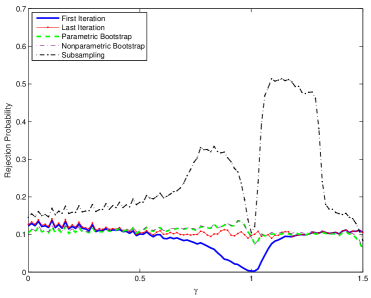
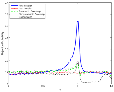
Figure 1 plots null rejection probabilities for $\rho=0.95$ and $\rho=-0.95$. Taking $c$ ranging from $-100$ to $50$ allows us to consider cases in which the regressors are stationary ($\gamma=0.00,...,0.50$), nearly integrated ($\gamma=0.85,...,0.95$), exactly integrated ($\gamma=1.00$), nearly explosive ($\gamma=1.05$ or $1.10$), and explosive ($\gamma=1.20,...,1.50$).

When $\rho=0.95$ and we include only the initial points $\gamma=0.5$ and $\gamma=1.2$, the null rejection probability is lower than 10% for values of $\gamma$ between the endpoints $\gamma=0.5$ and $\gamma=1.2$. The associated test seems to have correct size but the null rejection probability is near zero when $\gamma=1$. As a result, the power of a test using only the two endpoints can be very low when the series is nearly integrated. By adding additional points, the null rejection probability becomes closer to 10% for all values $\gamma\in\left[0.5,1.2\right]$. In practice, our algorithm includes about 10 additional points. When $\rho=-0.95$ and we consider only the initial points $\gamma=0.5$ and $\gamma=1.2$, the null rejection probabilities can be as large as 55%. Applied researchers would then reject the null considerably more often than the reported nominal level. By sequentially adding the most discrepant points, the algorithm eventually yields a null rejection probability close to 10%.

Figure 1 also compares the CVF approach with the usual bootstrap method, the parametric bootstrap, and subsampling. For the (nonparametric) bootstrap, we draw a random sample from the centered empirical distribution function of the fitted residuals for $\epsilon_{t}$ from OLS regressions. For the parametric bootstrap, we replace the unknown autoregressive parameter $\gamma$ with the OLS estimator. For the subsampling, we choose the subsampling parameters following the recommendation of Romano and Wolf [19]. The bootstrap sampling schemes have similar performance and do not have null rejection probability near 10% when the series are nearly integrated. This failure is due to the fact that the estimator $\widehat{\beta}$ is not locally asymptotically equivariant in the sense of Beran [3]; see also Basawa et al. [2]. The subsampling is a remarkably general method and has good performance when $\gamma=1$. However, its null rejection probability can be quite different from 10% for values of $\gamma$ near one. In the supplement, we show that the bootstrap and subsampling can be even further away from the nominal level of 10% if we make inference in the presence of a time trend.

Figure 2: Critical Value Function

(a) $\rho=0.95$

(b) $\rho=-0.95$

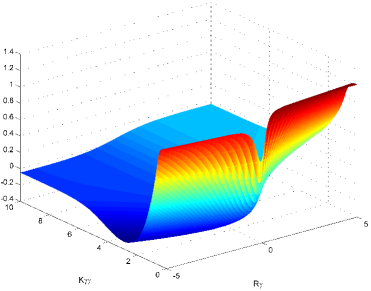
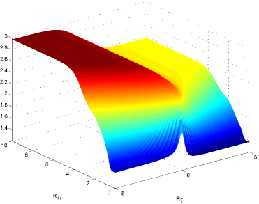
Interestingly, the null rejection probability for the CVF method is not far from 10% even for values of $\gamma$ outside the range $\left[0.5,1.2\right]$ whether $\rho$ is positive or negative. This suggests that the critical value functions take values close to 1.28, the 90% quantile of a standard normal distribution, when the series is stationary or explosive. Figure 2 supports this observation when the series is stationary. This graph plots the critical value function as a mapping of $R_{\gamma,T}\left(1\right)$ and $K_{\gamma\gamma,T}\left(1\right)$. To shorten notation, we denote these statistics $R_{\gamma}$ and $K_{\gamma\gamma}$ respectively. Standard asymptotic arguments show that $K_{\gamma\gamma}$ converges in probability to zero and $R_{\gamma}/K_{\gamma\gamma}$ diverges to $-\infty$. Whether $\rho=0.95$ or $\rho=-0.95$, the critical value function takes values close to 1.28 when $K_{\gamma\gamma}$ is close to zero and $R_{\gamma}$ is bounded away from zero (which, of course, implies that their ratio diverges). We cannot visualize, in this figure, the explosive case in which $K_{\gamma\gamma}$ diverges to $\infty$. In the supplement, we plot the critical values as a function of $R_{\gamma}/K_{\gamma\gamma}$ and $K_{\gamma\gamma}$ and re-scale the axis to accommodate for the explosive case as well. We show again that the critical value function takes values near 1.28 also when the series is explosive.

4.1 Size and Power Comparison

We now evaluate different size correction methods for the t-statistic when the variance matrix for the innovations $\varepsilon_{t}^{y}$ and $\varepsilon_{t}^{x}$ is unknown. The covariance matrix is estimated using residuals from OLS regressions.

We compare size and power of the similar t-test with the two other similar tests: the $L_{2}$ test of Wright [21] and the UMPCU test of Jansson and Moreira [10]. The figures present power curves for $c=-15$ and $c=0$. The rejection probabilities are plotted against local departures from the null hypothesis. Specifically, the parameter of interest is $\beta=b\cdot\sigma_{yy.x}\cdot g_{T}\left(\gamma\right)$ for $b=-10,-9,...,10$. The value $b=0$ corresponds to $\beta=0$ for the null hypothesis $H_{0}:\beta\leq 0$.

Figure 3 plots size and power comparisons for $\rho=0.95$. The similar t-test has correct size and null rejection probability near the nominal level when $b=0$. Hence, replacing the unknown variance by a consistent estimate has little effect on size in practice. Indeed, the limiting distribution of the t-statistic and the CVF is the same whether the variance is estimated or not. The $L_{2}$ test is also similar but does not have correct size when the series is integrated. The $L_{2}$ test actually has a bell-shaped power curve when the regressor is integrated, but has a monotonic power curve when the series is nearly integrated. This inconsistency makes it hard to use the $L_{2}$ test for either one-sided or two-sided hypothesis testing problems. Although the UMPCU test is a similar test, our reported null rejection probability is near zero when $b=0$ and the series is nearly integrated. This problem is possibly due to the inaccuracy of the algorithm used by Jansson and Moreira [10] for integral approximations (and their computed critical value).

Figure 3: Power ($\rho=0.95$)

(a) $\gamma=0.85$

(b) $\gamma=1$

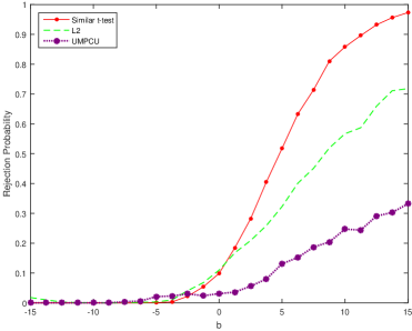
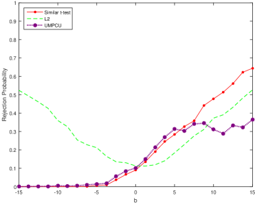
Whether the series is nearly integrated or exactly integrated, the similar t-test dominates the two other similar tests in terms of power. When $c=-15$ and $b=10$, the similar t-test has power above 90% while the $L_{2}$ and UMPCU tests have power lower than 60% and 30%, respectively. When $c=0$ and $b=10$, the similar t-test has power close to 50% while the $L_{2}$ and UMPCU tests have power close to 40% and 30%. The fact that the similar t-test outperforms the UMPCU test may seem puzzling at first. However, the UMPCU test is optimal within the class of similar tests conditional on specific ancillary statistics $S_{\beta\beta}$ and $S_{\gamma\gamma}$. As there exist similar tests beyond those considered by Jansson and Moreira [10], our less restrictive requirement yields power gains. Therefore, the performance of the similar t-test shows that the UMPCU test uses a conditional argument that entails unnecessary power loss.

The similar t-test also has considerably better performance than the other similar tests when the endogeneity coefficient is negative. Figure 4 presents power curves for $\rho=-0.95$. All three tests present null rejection probabilities near the nominal level when $b=0$. The $L_{2}$ test again can present bell-shaped power, and does not even have correct size. The power functions for the similar t-test and UMPCU test are monotonic and have null rejection probabilities smaller than 10% when $c=-15$ or $c=0$.

Figure 4: Power ($\rho=-0.95$)

(a) $\gamma=0.85$

(b) $\gamma=1$

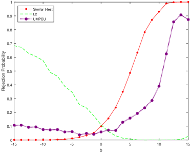
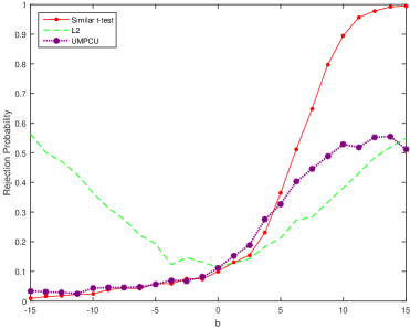
The supplement presents size and power comparisons for all combinations of $c=-100$, $-50$, $-15$, $0$, $10$, $30$ and $\rho=0.5$, $-0.5$, $0.95$, $-0.95$. These numerical simulations further show that the similar t-test has overall better performance than the $L_{2}$ and UMPCU tests in terms of size and power.

5 Conclusion and Extensions

This paper proposes a novel method to find tests with correct size for situations in which conventional numerical methods do not perform satisfactorily. The critical value function (CVF) approach is very general and relies on weighting schemes which can be found through linear programming (LP). Considering the polynomial speed of interior-point methods for LP, it is fast and straightforward to find the CVF. The weights are chosen so that the test is similar for a finite number of null rejection probabilities. If the nuisance parameter dimension is not too large, we expect the CVF method to work adequately.

In a model with persistent regressors, the CVF method yields a similar t-test which outperforms other similar tests proposed in the literature. It would be interesting to assess how our methodology performs in other models. For example, take the autoregressive model. If the model has one lag, Hansen [9] suggests a “grid” bootstrap which delivers confidence regions with correct coverage probability (in a uniform sense). This method relies on less restrictive conditions than the bootstrap. However, it requires the null distribution of the test statistic to be asymptotically independent of the nuisance parameter (hence, it is applicable even for our model with persistent regressors). If the autoregressive model has more lags, Romano and Wolf [19] propose subsampling methods based on Dickey-Fuller representations. Their proposed confidence region which has correct coverage level can be conservative (in the sense that some of the coverage probabilities can be larger than the nominal level). By inverting the tests based on the CVF method, we are able to provide confidence regions which instead have coverage probabilities near the nominal level.

References

- Anderson [1959] Anderson, T. W. (1959). On asymptotic distributions of estimates of parameters of stochastic difference equations. The Annals of Mathematical Statistics 30, 676–687.
- Basawa et al. [1991] Basawa, I. V., A. K. Mallick, W. P. McCormick, J. H. Reeves, and R. L. Taylor (1991). Bootstrapping unstable first-order autoregressive processes. Annals of Statistics 19, 1098–1101.
- Beran [1997] Beran, R. (1997). Diagnosing bootstrap success. Annals of the Institute of Statistical Mathematics 49, 1–24.
- Bickel and Freedman [1981] Bickel, P. J. and D. A. Freedman (1981). Some asymptotic theory for the bootstrap. Annals of Statistics 9, 1196–1217.
- Cavanagh et al. [1995] Cavanagh, C. L., G. Elliott, and J. H. Stock (1995). Inference in models with nearly integrated regressors. Econometric Theory 11, 1131–1147.
- Efron [1975] Efron, B. (1975). Defining the curvature of a statistical problem (with applications to second order efficiency). Annals of Statistics 3, 1189–1242.
- Efron [1978] Efron, B. (1978). The geometry of exponential families. Annals of Statistics 6, 362–376.
- Efron [1979] Efron, B. (1979). Bootstrap methods: Another look at the jackknife. Annals of Statistics 7, 1–26.
- Hansen [1999] Hansen, B. E. (1999). The grid bootstrap and the autoregressive model. Review of Economics and Statistics 81, 594–607.
- Jansson and Moreira [2006] Jansson, M. and M. J. Moreira (2006). Optimal inference in regression models with nearly integrated regressors. Econometrica 74, 681–715.
- Jeganathan [1995] Jeganathan, P. (1995). Some aspects of asymptotic theory with applications to time series models. Econometric Theory 11, 818–887.
- Jeganathan [1997] Jeganathan, P. (1997). On asymptotic inference in linear cointegrated time series systems. Econometric Theory 13, 692–745.
- Le Cam and Yang [2000] Le Cam, L. and G. L. Yang (2000). Asymptotics in Statistics: Some Basic Concepts. Second Edition. New York: Springer-Verlag.
- Mikusheva [2007] Mikusheva, A. (2007). Uniform inference in autoregressive models. Econometrica 75, 1411–1452.
- Moreira and Moreira [2013] Moreira, H. and M. J. Moreira (2013). Contributions to the theory of optimal tests. Ensaios Economicos 747. FGV/EPGE.
- Politis and Romano [1994] Politis, D. N. and J. P. Romano (1994). Large sample confidence regions based on subsamples under minimal assumptions. Annals of Statistics 22, 2031–2050.
- Politis et al. [1999] Politis, D. N., J. P. Romano, and M. Wolf (1999). Subsampling. New York: Springer Verlag.
- Romano and Shaikh [2012] Romano, J. P. and A. M. Shaikh (2012). On the uniform asymptotic validity of subsampling and the bootstrap. Annals of Statistics 40, 2798–2822.
- Romano and Wolf [2001] Romano, J. P. and M. Wolf (2001). Subsampling intervals in autoregressive models with linear time trend. Econometrica 69, 1283–1314.
- van der Vaart [1998] van der Vaart, A. W. (1998). Asymptotic Statistics. Cambridge: Cambridge University Press.
- Wright [2000] Wright, J. H. (2000). Confidence sets for cointegrating coefficients based on stationarity tests. Journal of Business and Economic Statistics 18, 211–222.