A Fast Algorithm for Finding Point Sources in the Fermi Data Stream: FermiFAST

Abstract

We present a new and efficient algorithm for finding point sources in the photon event data stream from the Fermi Gamma-Ray Space Telescope, FermiFAST. The key advantage of FermiFAST is that it constructs a catalogue of potential sources very fast by arranging the photon data in a hierarchical data structure. Using this structure FermiFAST rapidly finds the photons that could have originated from a potential gamma-ray source. It calcuates a likehihood ratio for the contribution of the potential source using the angular distribution of the photons within the region of interest. It can find within a few minutes the most significant half of the Fermi Third Point Source catalogue (3FGL) with nearly 80% purity from the four years of data used to construct the catalogue. If a higher purity sample is desirable, one can achieve a sample that includes the most significant third of the Fermi 3FGL with only five percent of the sources unassociated with Fermi sources. Outside the galaxy plane, all but eight of the 580 FermiFAST detections are associated with 3FGL sources. And of these eight, six yield significant detections of greater than five sigma when a further binned likelihood analysis is performed. This software allows for rapid exploration of the Fermi data, simulation of the source detection to calculate the selection function of various sources and the errors in the obtained parameters of the sources detected.

1 Introduction

The launch of the Fermi Gamma-Ray Telescope on 11 June 2008 brought dramatically more sensitive instruments to bear on the study of the Universe in gamma rays. The observations of the Fermi LAT (Large Area Telescope) (e.g. Ackermann et al., 2012) have resulted in a series of catalogues of point sources both within the Galaxy and beyond (e.g. Abdo et al., 2010; Ackermann et al., 2011; Nolan et al., 2012; Abdo et al., 2013; Ackermann et al., 2013; Acero et al., 2015). Both the identification of sources and their characterisation rely on the calculation of a likelihood ratio for the observed data with and without a source and for different characteristics for the potential source (Cash, 1979; Sutherland & Saunders, 1992; Mattox et al., 1996). These telescopes as well as Cerenkov telescopes on the ground rely on the conversion of gamma-rays into electron-positron pairs as they enter the telescope (or the atmosphere). By tracing the motion of these pairs, one can reconstruct the momentum of the incoming gamma ray. For low gamma-ray energies the reconstruction is poorer than at higher energies. Because of this broad point-spread function of gamma-ray telescopes the contribution of several potential sources will overlap in a particular region of the sky making the generation of a catalogue even more difficult and time consuming.

Although both Fermi and EGRET before it used the likelihood ratio to assess the significance of potential point sources, several alternatives have been proposed to search for point sources to account for the photons observed by these instruments. Massaro et al. (2009) and Campana et al. (2008) developed an algorithm to build a minimal spanning tree from the arrival directions of the photons over a large portion of the sky. They then divide the tree into subclusters by removing branches larger than a particular threshold. If a subcluster contains more than a particular number of photons, it is considered to be a potential point source. Campana et al. (2013) extended the technique to include a noisy background. Damiani et al. (1997a, b) and Ciprini et al. (2007) proposed to use wavelets to find point sources from photon counts for ROSAT, EGRET and Fermi data. Althoguh these techniques are significantly faster than the traditional likelihood ratio, they require simulated data to assess the significance of the sources detected because they do not rely of statistics with well understood distributions given the null hypothesis of no point source at a particular location. In general the estimated significances are proportional to those found in the full likelihood analysis.

In this paper we propose a technique to calculate likelihood ratios much more quickly that the usual techniques by storing the photon data stream in a data structure optimized for finding photons within a given percentile of the point spread function of the instrument from a potential source. Furthermore, we will assume a simple expression for the likelihood that assumes that the photons from within a particular region of the sky come from the combination of a point source at the centre of the region and a flat background. We do not assume a particular spectral model but only that the measured momenta of photons from a point source follow the expected distribution from a point source as determined by measurements and simulations (Ackermann et al., 2013).

2 The Photon Database

The key to the speed of this algorithm is the database that contains the positions of the observed photons on the sky. Each photon is stored in a four-dimensional $k-d$ tree (Bentley, 1975). A $k-d$ tree is a binary tree in which each successive branching splits the space in two regions along a hyperplane perpendicular to the last splitting. For example, to construct an efficient two-dimensional $k-d$ tree, we would first find the median $x$-coordinate of our points and assign it to be the root of the tree. The left branch would contain all the points with $x$ values less than the median, and the right branch would contain all the points with $x$ values greater than the median. Now we repeat the process with only the points on the left branch and use the $y$-coordinate instead of the $x$-coordinate, so we now have left-upper branch with $x$-values less than the median $x$-value and $y$-values greater than the median $y$-value for the points on the left branch. Similarly, we have a left-lower branch, and we repeat the process on the right branch, generating a right-upper and right-lower branches. The next step in the two-dimensional $k-d$ tree is to repeat on each of the branches with the $x-$coordinate again. The branching points do not have to be the precise medians of the data; one can construct well-balanced and efficient trees by sampling a fraction of the points to estimate the medians. The process continues until all the branches end with single points. Our photon data is four-dimensional. We use $x$, $y$ and $z$ to represent a photon’s position on the celestial sphere and $w$ to encode the 95%-energy-containment radius. Therefore, in our case, we construct a four-dimensional $k-d$ tree, so we split the data along a plane with constant $x-$coordinate, constant $y$, constant $z$, constant $w$ and then repeat with the $x-$coordinate. Once a $k-d$ tree is constructed for the data, one can search for points in our case photons within a given range of a particular position on the sky efficiently. Because the points are arranged in a binary tree, finding the photons that arrived within a given angle of a particular direction takes only on order of $\log_{2}N$ operations where $N$ is the total number of photons in the database.

We use the particularly memory efficient implementation of Lang (2009) (used in astrometry.net). The coordinates are actually stored as shorts instead of floats to save additional memory. The typical coordinates range from $-1$ to $+1$, so using shorts yields an angular precision of about six arcseconds much finer than that of the Fermi point-spread function (PSF). This memory efficient implementation allows us to store all the photons detected by Fermi above 100 MeV and within a zenith angle of 100 degrees in memory simultaneously. The first three dimensions contain the position of the photon on the celestial sphere as shown in the upper portion of Fig. 1. Storing the direction of the photon momentum in this manner removes the coordinate singularity of the spherical coordinates. The fourth coordinate that we denote by $w$ depends on the point-spread function for the photon in question. In particular $w=\pm\sqrt{R^{2}_{\mathrm{max}}-R_{i}^{2}}$ where $R_{i}$ is the radius of the ninety-fifth percentile at the energy, entrance angle and front or back conversion for the photon. The choice of the ninety-fifth percentile is arbitrary. Choosing a smaller cut-off radius would decrease the number of photons from the candidate point source and also from the background. For convenience, we use positive values of $w$ for front-converted photons and negative values of $w$ for back-converted photons. Furthermore, $R_{\mathrm{max}}$ is the largest value of the ninety-fifth percentile of all the photons in the sample, i.e. the ninety-fifth percentile for the photon with the poorest angular resolution. This is depicted in the lower panel of Fig. 1.

Figure 1: The location of a given photon event on the celestial sphere and in the additional dimension. $R_{i}$ is the ninety-fifth percentile radius for the photon in question and $R_{\mathrm{max}}$ is the largest ninety-fifth percentile radius for the photons in the sample.

Once the $k-d$ tree is created, it is efficient to find all the entries within the database within a given Cartesian distance of a particular point. In our case we query the database for all the photons within a distance $R_{\mathrm{max}}$ of a particular point on the celestial sphere and use $w=0$ for the fourth coordinate. The particular choice of $w$ for the observed photons means that the query will yield all the photons that are within the ninety-fifth percentile of the PSF. In other words, if there is a point source located at that particular point the query will return on average 95% of the photons from that source. Of course, it will also return photons from the background and other nearby sources. Additionally, the region of interest for a particular prospective source is energy dependent. The form of the exposure map also is energy dependent as shown in Fig. 2. It peaks at 0.95 times the exposure time in the direction of the potential source and slowly drops to the ninety-fifth percentile of the PSF in radius and then drops according to the power-law of the tail component of the linear combinations of King functions,

$$K(\delta p;\sigma,\gamma)=\frac{1}{2\pi\sigma^{2}}\left(1-\frac{1}{\gamma}\right)\left[1+\frac{1}{2\gamma}\left(\frac{\delta p}{\sigma}\right)^{2}\right]^{-\gamma}$$ (1)

that are used to characterise the Fermi PSF (Ackermann et al., 2013).

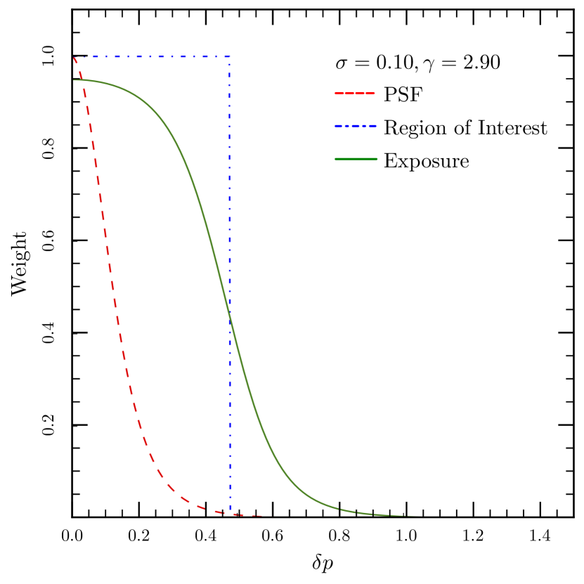
Figure 2: The Exposure Map, Region of Interest (ROI) and Point-Spread Function (PSF) with $\sigma$ and $\gamma$ characterise the width of the King function and its asymptotic power-law dependence respectively according to Eq. 1.

Although the construction of the tree is not done in parallel, the queries are performed in parallel using the tree held in shared memory. For example if one uses all the photons above 100 MeV from weeks 9 through 216 with a standard zenith angle cut of less than 100 degrees (89,684,009 photons) requires one gigabyte to store the tree and about ten minutes to construct. We perform 200,000 location queries corresponding to a HEALPix (Górski et al., 2005) grid with $\mathtt{NSIDE}=128$ (see § 3 for further details). The 200,000 location queries and likelihood calculations require 140,000 seconds (700 ms each), so the speed-up through parallisation can be dramatic. On the other hand, if one restricts to photons above 1 GeV (13,193,171), it only takes 90 seconds to construct the tree. At higher energies, it makes sense to make more location queries because the PSF is smaller. In this example 786,426 queries require 5,600 seconds of CPU time (7 ms each) or only six minutes on sixteen cores.

3 Source Likelihood

Using the $k-d$ tree to determine the photons that lie within the 95% energy enclosure region of the point-spread function, we calculate several statistics of the observed photons to assess the likelihood of a source being at a particular position on the sky. We first determine two statistics whose distributions are potentially known. First, if all the photons within the region of interest (all photons that lie within the 95th-percentile cone of the potential source) indeed come from a uniform background, we would expect that the photons would be uniformly distributed in the region of interest. Therefore, in this case the ratio of the solid angle enclosed in a circle centred on the potential source and running through the observed photon to the total solid angle within the region of interest for that particular photon should be uniformly distributed between zero and one. This is just a $V/V_{\mathrm{max}}$-test (Schmidt, 1968) adapted to the distribution of the photons on the sky.

We denote the mean of this ratio over the observed photons $\bar{r}^{2}$, that is

$$\bar{r}^{2}=\sum_{i}\left(\frac{r_{i}}{r_{\mathrm{max},i}}\right)^{2}$$ (2)

where $r_{i}$ is the angular distance between the photon direction and the direction of the potential source and $r_{\mathrm{max},i}$ is the 95% energy containment radius for the photon. This statistic is distributed as a Bates distribution with mean of $1/2$ and variance of $1/(12N_{\gamma})$.

Second, if all the photons within the region of interest indeed come from a point source at the centre of the region of interest that extends to the ninety-five percentile, the ratio of the percentile of a given photon within the cumulative PSF distribution for that particular photon to 0.95 should be uniformly distributed between zero and one. For convenience because we only probe the photons out to the 95% energy containment radius, we define the cumulative fraction of energy out to the ninety-fifth percentile

$$C_{\mathrm{PSF}}(r)=\frac{1}{0.95}\int_{0}^{r}\mathrm{PSF}(r^{\prime})2\pi r^{\prime}dr$$ (3)

and

$$\bar{f}=\sum_{i}C_{\mathrm{PSF}}(r_{i}).$$ (4)

This will be distributed as a Bates distribution if all of the photons come from a point source.

If we assume that the observed photons originate from a linear combination of these two possiblities, we can determine the ratio of the two contributions from these statistics. For $\bar{r}^{2}$ we have

$$\bar{r}^{2} = A_{f}\int_{0}^{1}\left(\frac{r}{r_{\mathrm{max}}}\right)^{2}d\left(C_{\mathrm{PSF}}\right)+$$

$$~{}~{}~{}(1-A_{f})\int_{0}^{1}\left(\frac{r}{r_{\mathrm{max}}}\right)^{2}d\left(\frac{r}{r_{\mathrm{max}}}\right)^{2}$$

and for $\bar{f}$ we have

$$\bar{f} = A_{f}\int_{0}^{1}C_{\mathrm{PSF}}d\left(C_{\mathrm{PSF}}\right)+$$

$$~{}~{}~{}(1-A_{f})\int_{0}^{1}C_{\mathrm{PSF}}d\left(\frac{r}{r_{\mathrm{max}}}\right)^{2}.$$

To move forward we examine the first term in $\bar{r}^{2}$

$$B = \int_{0}^{1}\left(\frac{r}{r_{\mathrm{max}}}\right)^{2}d\left(C_{\mathrm{PSF}}\right)=\left.\left(\frac{r}{r_{\mathrm{max}}}\right)^{2}C_{\mathrm{PSF}}\right|_{0}^{1}-$$

$$~{}~{}~{}\int_{0}^{1}C_{\mathrm{PSF}}d\left(\frac{r}{r_{\mathrm{max}}}\right)^{2}.$$

$$= 1-\int_{0}^{1}C_{\mathrm{PSF}}d\left(\frac{r}{r_{\mathrm{max}}}\right)^{2}$$ (8)

where we have integrated the first term by parts to get one minus the second term in $\bar{f}$. We can substitute these results into Eq. 3 and 3 to yield

$$\bar{r}^{2} = A_{f}B+\frac{1-A_{f}}{2}$$ (9)

$$\bar{f}^{2} = \frac{A_{f}}{2}+(1-A_{f})(1-B)$$ (10)

Using this result, we can solve for the fraction of photons that come from the point source to yield

$$A_{f}=\frac{\frac{1}{2}-\bar{r}^{2}}{\bar{f}-\bar{r}^{2}}.$$ (11)

We can also find the value of $B$ to be

$$B=\bar{r}^{2}-\bar{f}+\frac{1}{2}.$$ (12)

The estimator $A_{f}$ is calculated from various statistics of the sample and assumes that the photons come from a single point source and a flat background, so it can have sampling errors that cause it to be out of the range of 0 to 1, and systematics errors as well (e.g. the photons come from multiple sources) that can also put it out of this range. We can estimate the significance of the value of $A_{f}$ by

$$S(r^{2})=\left(\bar{r}^{2}-\frac{1}{2}\right)\sqrt{12N_{\gamma}}.$$ (13)

We have retained the sign of the deviation from the source-free value, so that a negative value of $S(r^{2})$ indicates that the photons within the region of interest are centrally concentrated. The probabilty of getting a value of $|S(r^{2})|$ larger than $x$ by chance is

$$P\left[|S(r^{2})|>x\right]=\frac{1}{2}\mathrm{erfc}\left(\frac{x}{\sqrt{2}}\right)\approx\exp\left(-\frac{x^{2}}{2}\right)$$ (14)

if we take the limit of many photons in the region of interest where the Bates distribution tends to the normal distribution.

Table 1: Basic statistics calculated for the photon distribution around a potential source

Statistic	Symbol	Abbreviation	Definition
Number of photons	$N_{\gamma}$	N	Number of photons that lie within the 95% percentile
Mean Solid Angle Ratio	$\bar{r}^{2}$	MEANR2	The mean of the ratio of solid angle enclosed between observed
			photon position and source location and the solid angle
			enclosed with the 95% percentile of the PSF
Mean Percentile Ratio	$\bar{f}$	MEANFRAC	The mean of the ratio of PSF percentile to 95%
Significance of MEANR2	$S(r^{2})$	SIGR2	How many standard deviations is MEANR2 away from 0.5
Significance of MEANFRAC	$S(f)$	SIGFRAC	How many standard deviations is MEANFRAC away from 0.5
Fraction of photons from point source	$A_{f}$	AFRAC	If one assumes that the photons come from the sum of a
			uniform background and a point source, what fraction
			come from the point source? $A_{f}=(0.5-\bar{r}^{2})/(\bar{f}-\bar{r}^{2})$
Amplitude of PSF in Likelihood Fit	$A_{\mathrm{PSF}}$	APSF	Fraction of photons from the region of interest that come
			from the source according to the likelihood fit

These basic statistics are summarized in Tab. 1, and Tab. 2 lists these statistics for the fifteen most significant sources detected. These basic statistics really just compare two numbers about the distribution of the photons within the region of interest. We can use the detailed knowledge of the point spread function to develop a more comprehensive test of the distribution of photons. In particular, we define the unbinned likelihood (this is very similar to the expression used by Braun et al., 2008, for neutrino telescopes)

$$\log L=\sum_{\gamma}\log\left[A_{\mathrm{PSF}}\frac{\mathrm{PSF}_{i}\Omega_{\mathrm{max},i}}{0.95}+(1-A_{\mathrm{PSF}})\right]$$ (15)

where we have dropped $N_{\mathrm{pred}}$ from the usual definition because we have defined the model in such a way that $N_{\mathrm{pred}}=N_{\gamma}$ automatically and $dN_{\mathrm{pred}}/dA_{\mathrm{PSF}}=0$. The variable $\Omega_{\mathrm{max,i}}$ is the solid angle that encloses 95% of energy for the PSF of that particular photon, and $\mathrm{PSF}_{i}$ is the value of the PSF for the photon if it indeed comes from the position of the candidate source. The maximum of $\log L$ is found by numerically varying the value $A_{\mathrm{PSF}}$. For $A_{\mathrm{PSF}}=0$, $\log L=0$ and because we are fitting a single variable, $\log L$ is distributed as a chi-squared distribution with a single degree of freedom and the probability of getting a value of $\log L$ larger than $x$ by chance is

$$P(\log L>x)=\sqrt{\pi}\mathrm{erfc}\left(\sqrt{\frac{x}{2}}\right)\approx\exp\left(-\frac{x}{2}\right).$$ (16)

From Tab. 2 we can see that the values of $A_{f}$ are similar to those of $A_{\mathrm{PSF}}$ at least for highly significant sources.

The first pass is to determine the value of $\log L$ on a HEALPix grid (Górski et al., 2005) of potential sources. The HEALPix grid is an array of equal area regions on a sphere, in this case the sky. The sphere is first projected onto a rhombic dodecahedron. Each of the faces is a rhombus congruent to the others, and a pair of opposite vertices is aligned with the poles. Each of the rhombuses is subdivided into equal solid angle regions by dividing in each dimensional in two. The parameter $\mathtt{NSIDE}$ is the number of subdivisions and must be a power of two, so the total number of regions is $12\times\mathtt{NSIDE}^{2}$.

In the FermiFAST algorithm we use the HEALPix grid for the initial guesses for source positions and to find local maxima on the grid. Once the approximate local maxima are found on the grid, we refine the position of the detection to increase the likelihood further. Consequently, the initial spacing of the grid should be smaller than the angular resolution of the LAT at the energy range of interest, so that separate sources result in separate peaks in the initial likelihood map. Otherwise, the value of $\mathrm{NSIDE}$ is arbitrary. For example for the photons above 1 GeV we used $\mathtt{NSIDE}=256$ or 786,432 grid points, so the grid points lie approximatly 13 arcminutes apart or about twenty points per square degree and 60 measurements within the typical 68% energy containment radius at 1 GeV (Ackermann et al., 2012). Of these 786,432 points, 18,425 have $P(\log L>x)<e^{-12.5}\approx 4\times 10^{-6}$. This is a five-sigma threshold. Next we take this list of potentially significant sources and find the local maxima of $\log L$; this reduces the number to 1,226 unique potential sources. However, 426 have $A_{\mathrm{PSF}}<0$, indicating not a source but a point-like deficit, leaving 800 sources. Each of these potential source positions is used as an initial guess to optimize the local maxima of $\log L$ and get a more precise position for each source. For the lower-energy cutoff, we start with $\mathtt{NSIDE}=128$ or 196,608 grid points or a separation of 26 arcminutes. Of these 196,608 points, 96,066 have $P(\log L>x)<e^{-12.5}\approx 4\times 10^{-6}$ and 967 unique peaks of which 310 have $A_{\mathrm{PSF}}>0$.

Before discussing the results (i.e. the catalogue of sources) and how they compare with the third Fermi catalogue, we will examine the performance of the technique and focus on the sources detected from photons with energies exceeding 1 GeV. The left-panel of Fig. 3 depicts the results of the initial set of peaks with $P(\log L)<e^{-12.5}$ before position refinement. We see that for $A_{f}>0$ there is a strong linear correlation between the value of $A_{f}$ and $A_{\mathrm{PSF}}$. Whereas for negative values of $A_{f}$ where there is a hole in the photon distribution, the value of $A_{\mathrm{PSF}}$ saturates at $-0.1$. The right panel shows the values of $A_{\mathrm{PSF}}$ against the significance. There are both significant sources and holes in the photon distribution. The fractional deficit in the “hole” regions is limited to one tenth. Because of the focus of this paper is to look for gamma-ray sources, we will not discuss these “holes” further, but they would be an interesting focus of further investigation.

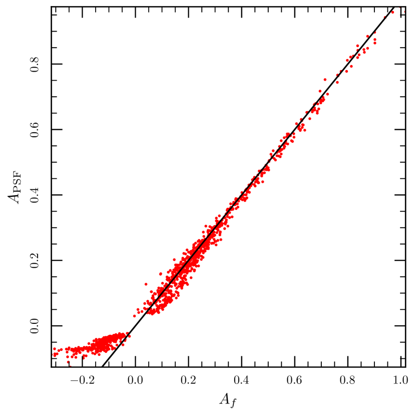
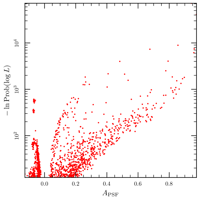
Figure 3: Left: the correlation of the value $A_{f}$, determined from the means of the photon distributions, to the value of $A_{\mathrm{PSF}}$, determined from the maximum likelihood techinque. The line traces $A_{\mathrm{PSF}}=A_{f}$. Right: The values of $A_{\mathrm{PSF}}$ against the significance.

For the sources in the preliminary catalogue (i.e. those with $A_{\mathrm{PSF}}>0$) we further refine the position estimate of the source. The left panel of Fig. 4 depicts the change in $\log L$ during the optimization. Sometimes the value of $\log L$ actually decreases, but usually it increases modestly by say ten percent. The right panel shows the change in the position of the source. The size of each HEALPix region is about 0.2 degrees on a side, so an optimization within a given HEALPix cell would result in a typical movement of about one tenth of a degree, and the results bear this out. Occasionally the estmated source position moves by a large distance indicating that the optimization has found another nearby peak. We use the optimized position only if the value of $\log L$ has actually increases, and the estimated position of the source has shifted by less than 0.5 degrees.

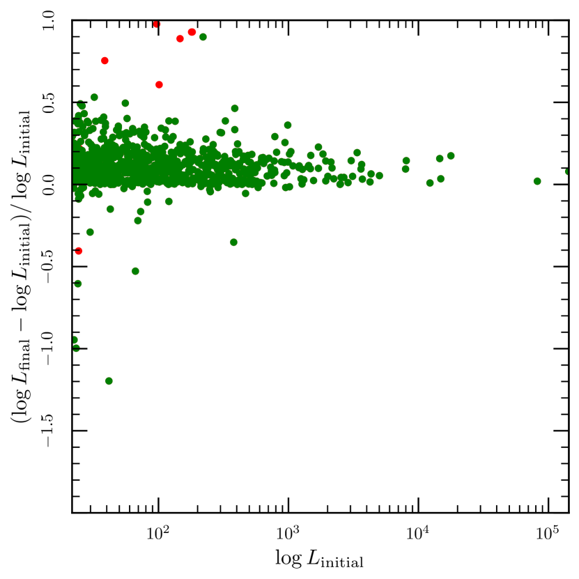
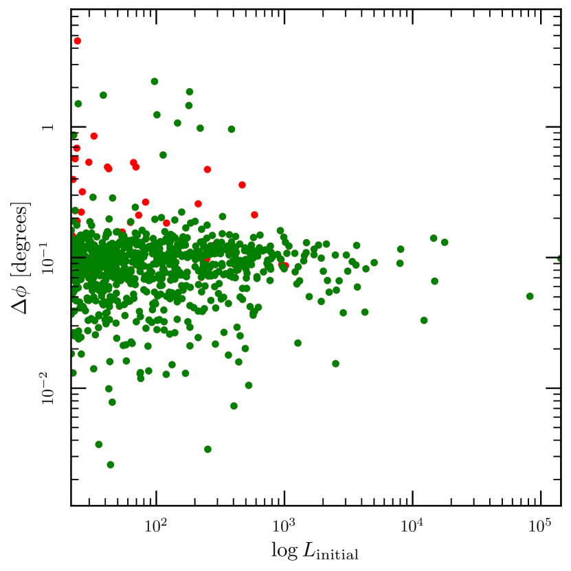
Figure 4: Left: the relative change in $\log L$ during the position refinement. Green is for sources whose positions moved less than one degree. Red is for greater movement. Right: the relative change in position during the position refinement. Green is for sources whose positions likelihood increased. Red is for those whose likelihood decreased.

4 Results

To test the algorithm we used nearly the same data set as used to construct the Fermi Large Area Telescope Third Source Catalog (3FGL Acero et al., 2015). We used weeks 9 through 216. That is, photons detected between 2008 August 4 (15:45:36 UTC) and 2012 July 26 (01:07:25 UTC), a span of nearly four years. This is about five days shorter than the span of the 3FGL observations because we used the weekly files. We used the good-time intervals (GTI) as defined by the Fermi team, the Pass 7 response function (P7REP_SOURCE_V15) and the Pass 7 reprocessed data. We use the Pass 7 data for comparison with the analysis of the 3FGL which also used Pass 7 data. From the form of the likelihood function, Eq. 15, it is apparent that we do not use a model for the background, and the key ingredient of the instrument response is the estimate of the point-spread function (Ackermann et al., 2012).

We create two catalogues: one using photons above 1 GeV and the second with all photons above 100 MeV. The fifteen most significant sources in the 1 GeV map are given in Tab. 2 with the refined positions and the original detection significances. We see a general trend that the significances in sigma-units of the 3FGL are about three times that of the FermiFAST technique. The two exceptions in the table are the Crab pulsar and 3FGL J1745.6-2859c/3FGL J1745.3-2903c. The Fermi analysis splits the Crab source among three sources: the pulsar itself, the synchrotron and inverse Compton components of the pulsar wind nebulae. The FermiFAST source most closely coincides with the pulsar, and the 3FGL significance for this component alone is quoted in the table. The thirteenth FermiFAST source lies close to both 3FGL J1745.6-2859c (1.8 arcminutes) and 3FGL J1745.3-2903c (7.1 arcminutes). It is closer to 3FGL J1745.6-2859c which has a lower 3FGL significance than the other potential counterpart.

Table 2: The results for the fifteen most significant peaks in the 1 GeV map. We list two entries for the thirteenth source because there are two 3FGL sources within 6 arcminutes of each and the FermiFAST source. The closer source to the FermiFAST detection is listed first.

Source	RA	Dec	$N_{\gamma}$	$\bar{r}^{2}$	$\bar{f}$	$S(r^{2})$	$S(f)$	$A_{f}$	$A_{\mathrm{PSF}}$	$S(\mathrm{FF})$	$S(\mathrm{3FGL})$
PSR J0835-4510 (Vela)	$128.84$	$-45.18$	171821	$0.174$	$0.521$	$-467.5$	$29.5$	$0.94$	$0.94$	$378.92$	$1048.96$
PSR J0633+1746 (Geminga)	$98.48$	$17.77$	90467	$0.164$	$0.501$	$-349.9$	$0.6$	$1.00$	$0.97$	$286.73$	$1012.14$
PSR J0534+2200 (Crab)	$83.64$	$22.02$	26443	$0.204$	$0.558$	$-166.7$	$32.6$	$0.84$	$0.86$	$133.34$	$30.67$
LAT PSR J1836+5925	$279.06$	$59.43$	16595	$0.167$	$0.494$	$-148.8$	$-2.5$	$1.02$	$0.96$	$121.85$	$438.12$
PSR J1709-4429	$257.42$	$-44.48$	32526	$0.265$	$0.614$	$-146.9$	$71.3$	$0.67$	$0.68$	$121.02$	$360.82$
3C 454.3	$343.50$	$16.15$	14021	$0.170$	$0.511$	$-135.4$	$4.4$	$0.97$	$0.96$	$110.98$	$480.74$
LAT PSR J0007+7303	$1.76$	$73.05$	13558	$0.224$	$0.564$	$-111.5$	$25.6$	$0.81$	$0.79$	$89.89$	$288.75$
LAT PSR J2021+4026	$305.39$	$40.45$	31304	$0.331$	$0.669$	$-103.8$	$103.9$	$0.50$	$0.48$	$89.31$	$237.05$
PSR J1057-5226	$164.49$	$-52.46$	8194	$0.230$	$0.570$	$-84.6$	$21.8$	$0.80$	$0.78$	$70.87$	$200.06$
PSR J2021+3651	$305.26$	$36.85$	22683	$0.355$	$0.693$	$-75.5$	$100.5$	$0.43$	$0.41$	$65.78$	$145.14$
LS I+61 303	$40.14$	$61.22$	14060	$0.323$	$0.667$	$-72.6$	$68.5$	$0.51$	$0.51$	$65.12$	$196.61$
PKS 1510-08	$228.21$	$-9.10$	5718	$0.217$	$0.555$	$-74.0$	$14.5$	$0.84$	$0.82$	$60.86$	$207.27$
3FGL J1745.6-2859c	$266.45$	$-28.99$	48087	$0.388$	$0.750$	$-85.3$	$189.8$	$0.31$	$0.26$	$60.60$	$11.97$
3FGL J1745.3-2903c											$20.66$
PKS 0537-441	$84.71$	$-44.09$	4692	$0.188$	$0.534$	$-74.1$	$8.1$	$0.90$	$0.90$	$60.15$	$219.16$
Mkn 421	$166.12$	$38.21$	4527	$0.187$	$0.545$	$-73.0$	$10.5$	$0.87$	$0.89$	$58.16$	$190.35$

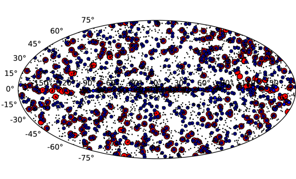
Figure 5: Sources with $\ln P(\log L)<-12.5$ (i.e. five sigma) in the 1 GeV catalogue (small blue circles), in the 100 MeV catalogue (big red circles) and the 3FGL (black dots).

All of the sources detected by FermiFAST above five-sigma in the 1 GeV and the 100 MeV sample are depicted in Fig. 5. One can see that nearly all of the FermiFAST sources correspond to 3FGL sources and in fact a few may correspond to several sources. On the other hand, there are many 3FGL sources that do not have counterparts in the FermiFAST catalogue. We can examine the statistics of the correspondances more carefully by examining the distance across the sky between the nearest neighbours in each of the two catalogues: FermiFAST and 3FGL. These are plotted as the red curves in Fig. 6 and the dashed red curve is a multi-Rayleigh distribution fit to the red curves. We assume a Rayleigh distribution to account for normally distributed errors in both directions along the sky. We find that the nearest neighbour in the 3FGL of almost all sources in the FermiFAST catalogue lies within about 1-2 arcminutes. We must assess whether these are chance coincidences. If the sources in the two catalogues are not correlated with each other (i.e. there are no real counterparts), then one would expect that the cumulative distribution of nearest neighbour distances to grow as a $1-\exp(\lambda\Omega)$ where $\lambda$ is the density of sources on the sky and $\Omega$ is solid angle enclosed by a circle centred on the object and passing through the nearest neighbour. Given that there are 3,029 Fermi 3FGL sources on the sky, the cumulative distribution in this case would approximately be $1-\exp(-r^{2}/2\sigma^{2})$ where $\sigma\approx 1.5^{\circ}$, so it is unlikely that these counterparts at a typical distance of 1 arcminutes are by chance.

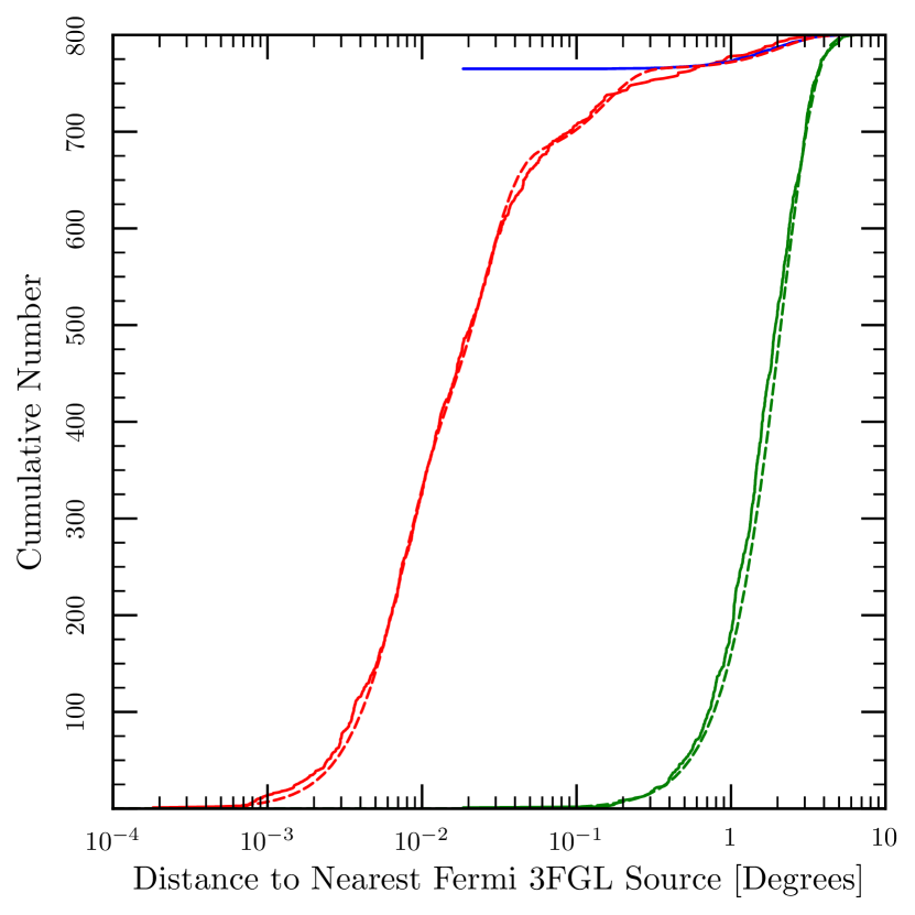
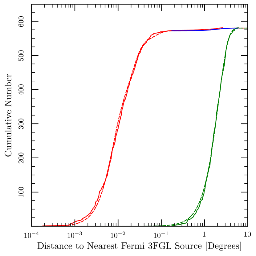
Figure 6: The left panel gives the results for all sources, and the right panel has $|b|>10^{\circ}$. The distance from a Fermi FAST source to the nearest Fermi 3FGL source. This demonstrates that ninety percent of the Fermi FAST sources are associated with sources in the Fermi 3FGL (across the whole sky) and nearly all at Galactic latitudes greater than ten degrees. The solid red curves give the observed cumulative distribution of nearest distances. The solid green curves give the cumulative distribution that one would expect if there were no associated between the Fermi FAST and Fermi 3FGL sources. This is calculated by performing the same analysis as the red curves but with the Galactic coordinates inverted. The blue curve yields the false positive rate. The dashed red and dashed green curves are Rayleigh distributions that are fit to the observed distributions. The typical positional error between associated 3FGL and FAST sources is 1-2 arcminutes.

We also can determine the distribution of unassociated pairs from the data itself by inverting the coordinates of the sources in one catalogue and looking for the nearest neighbours again. To be precise we change the sign of the Galactic latitude and longitude of each source in the 3FGL and repeat the nearest neighbour search. We invert the coordinates instead of assigning random positions in order to preserve the clustering of the sources on the sky and the density in Galactic latitude and longitude. Here all the correspondances are by chance. These results are given by the green curves in the various panels and let us assess that nearly all the sources in the FermiFAST have counterparts in the 3FGL. In the all-sky map (left panel, we can assess the number of FermiFAST sources that are not in the 3FGL by fitting the cumulative distribution with several Rayleigh distributions that quantify the positional error for the true counterparts and the chance of a false counterpart determined by fitting the cumulative distribution of false counterparts with a Rayleigh distribution as well. The distribution of false counterparts (green curves in Fig. 6) is well characterised by a Rayleigh distribution with $\sigma=1.5^{\circ}$ (magenta curves) as expected from the distribution of Fermi sources on the sky. We find that 35 of the 800 sources do not have a counterpart in 3FGL. If we now focus on the right panel of Fig. 6 we find that out of the 580 high-latitude sources in FermiFAST only eight lack a counterpart in 3FGL.

One thing that is glaringly obvious from Fig. 5 is that most sources in the 3FGL lack a counterpart in the FermiFAST catalogue, in both the 1 GeV and the 100 MeV versions. Given that the algorithm outlined here is much less comprehensive that the techniques used to generate the Fermi catalogues (there is no modelling of the background, multiple sources or spectra), this is not surprising. However, it is useful to figure out what sources are missing from the FermiFAST catalogue and why. Fig. 7 shows the relationship between the significances of a source assigned by FermiFAST and by the 3FGL. In particular the 3FGL significances are three times larger (the upper line) than FermiFAST typically, so if both apply a threshold of five-sigma, FermiFAST will find fewer sources. However, there is a large population of sources for which the two likelihoods are similar or the FermiFAST likelihood is larger. Since FermiFAST does not perform any spectral modelling, perhaps these sources have poor spectral fits in the 3FGL, yielding smaller likelihoods. Furthermore, this indicates a discovery space for FermiFAST to find point sources where we do not have a good prior notion of the spectral model. The rightmost outlying point in the lower-right is the Crab pulsar whose 3FGL likelihood is artificially too low due to the way it is fit within the catalogue. The second rightmost point is 3FGL J1745.6-2859c. It is likely that FermiFAST has combined the significance of this 3FGL source with the nearby source 3FGL J1745.3-2903c. The latter source has a 3FGL significance of 20.6.

To understand further whether FermiFAST is simply missing less significant 3FGL sources we can look at the cumulative distribution of 3FGL significances of sources that appear in the FermiFAST 1 GeV catalogue and all the 3FGL sources in Fig. 8. We see that FermiFAST catalogue is essentially complete for all 3FGL sources above about 18-sigma, so FermiFAST can quickly (in six minutes) generate a sample from the Fermi data stream of the upper quartile of sources that would appear a Fermi catalogue using the full likelihood technique to construct the catalogue.

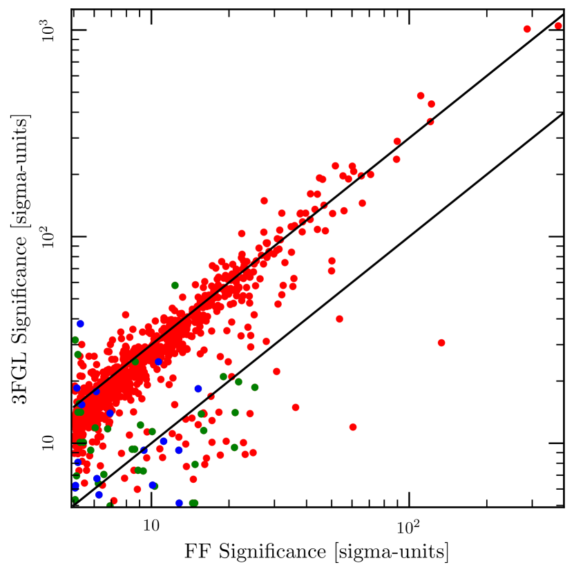
Figure 7: 3FGL Significances vs FermiFAST. The red points are where the counterparts lie within $0.2^{\circ}$ of each other, the green the counterparts lies between $0.2^{\circ}$ and $1^{\circ}$, and the blue have counterparts further than $1^{\circ}$ away. The upper line traces a 3FGL signifance three times larger than the FermiFAST significance. The lower line traces equal significance for the two techniques.

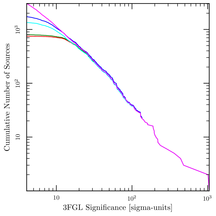
Figure 8: Cumulative distribution of 3FGL significances for the entire 3FGL (blue) and the entire FermiFAST 1-GeV catalogue with a five-sigma cut (green) and FermiFAST where the 3FGL counterpart lies within $0.2^{\circ}$ (red) again with a five-sigma cut. The blue and cyan give the same as green and red but with a three-sigma cut.

The question arises: is it possible to do better? We can reduce the significance threshold for find sources in the 1-GeV FermiFAST catalogue. We expect that the number of sources that do not have firm associations in the 3FGL to increase but also for the completeness to increase as well. We can use the empirical distance distribution for the false matches depicted in yellow in Fig. 9 to split the distribution of the matches between FermiFAST and the 3FGL statistcally into the true matches and the false matches to measure the completeness and purity of the samples. To do this we assume that all the true matches are closer than any of the false matches and use a ranked-sum-test to determine the fraction of true matches from the observed distribution of matches (see Appendix for details). For the 1-GeV catalogue this appears to be a good assumption. The contribution of the false matches to the cumulative distributions is depicted in the same colour as the measured distributions but dashed. The distribution of the close matches here is somewhat different from that in Fig. 6 because we have not used the improved localizations to find the matches. The localization improvement tends to fail more often for sources of low significance (see Fig. 4). Tab. 3 gives the results of this trial. The key result is that the five-sigma sample is very pure; only about five percent of the sources lack firm associations in the 3FGL. On the other hand, if one is willing to sacrifice the purity of the sample, one can achieve nearly 50% completeness relative to the 3FGL by reducing the significance threshold to $3-\sigma$. Fig. 8 shows by accepting a lower purity one can get a complete 3FGL sample to about ten-sigma, comprising nearly half of the 3FGL sample.

Table 3: Completeness and Purity

Threshold	Sources	True	False	Purity	Comp
$3-\sigma$	1727	1374	352	79.8%	48.4%
$3.5-\sigma$	1312	1178	134	89.8%	41.8%
$4-\sigma$	1076	1009	67	93.8%	36.2%
$4.5-\sigma$	923	877	46	95.1%	31.3%
$5-\sigma$	800	765	35	95.8%	27.0%

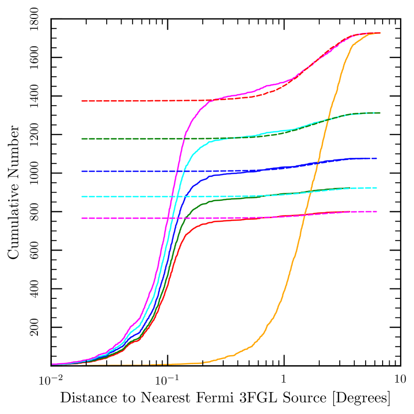
Figure 9: The cumulative distribution of distances between sources in FermiFAST and 3FGL for various significance thresholds from top to bottom of 3-sigma, 3.5-sigma, 4-sigma, 4.5-sigma and 5-sigma. The dashed curves that start above zero and join each cumulative distribution at large radii trace the cumulative distribution of distances for the false matches in each sample.

We saw in Fig. 7 that in general the FermiFAST significances and the 3FGL significances are well correlated. However, for about one fifth of the sources $S(\mathrm{3FGL})<2S(\mathrm{FF})$ and for about one tenth $S(\mathrm{3FGL})<S(\mathrm{FF})$. This demonstrates that at least for a fraction of the 3FGL the FermiFAST technique is more sensitive, so the sources that do lie in the FermiFAST catalogue but not the 3FGL may just be a class of sources to which the 3FGL is less sensitive, perhaps sources for which the suite of spectral models employed in the construction of the 3FGL do not apply. On the other hand, these unassociated sources could simply be regions where the diffuse background is especially bright and clumpy. Because the FermiFAST technique assumes that the background is smooth on the scale of the PSF, it would find a source where the background is locally strong. We possibly see the opposite of this effect in Fig. 3 where FermiFAST finds negative sources that are most likely places where the background is locally weak.

It is apparent from Fig. 5 that there are fewer 100-MeV sources and that most of these sources coincide with 3FGL and 1-GeV FermiFAST sources. In Fig. 10 the localization is slightly poorer than Fig. 9 because we have used a coarser HEALPix grid to sample the likelihoods. Moreover, for the 100-MeV catalogue we have not optimized the likelihood to determine more accurate positions because the optimization often drifts onto other nearby detections for the more poorly localised low-energy photons. Consequently, Fig. 9 is the best comparison not Fig. 6. Again we have used a rank-sum test to determine the sources that are likely to be shared between the catalogues and also to determine those sources that appear in the 100-MeV catalogue but not the others. The 100-MeV catalogue contains 312 sources of which 23 are in the 3FGL but not the 1-GeV catalogue, 16 are in the 1-GeV catagloue but not the 3FGL and 24 are in neither of the other catalogues (249 are in all three). Relative to the 3FGL catalogue the purity is 88.1% and the completeness is 12.1%. If one takes the union of the five-sigma 1-GeV and the five-sigma 100-MeV FermiFAST catalogues, there is a total of 788 sources that correspond to 836 3FGL sources (i.e. one FermiFAST source can correspond to several 3FGL sources) for a slightly higher completeness fraction of 27.6% than that of the five-sigma 1-GeV FermiFAST catalogue.

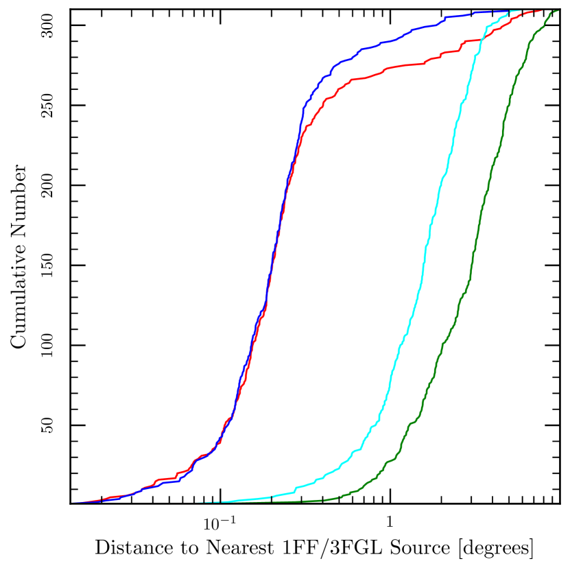
Figure 10: The cumulative distribution distances between sources in the 100-MeV catalogue and the 3FGL (blue, leftmost and higher) and the 1-GeV catalogue (red, second from left) and for the false matches between the 100-MeV and 3FGL (cyan, second from right) and 100-MeV and 1-GeV catalogue (green, rightmost).

A final test that we perform is to examine the high-significance FermiFAST detections that do not lie near sources within the 3FGL. There are thirty-five of these detections. The majority of these detections (27) lie within 10 degrees of the Galactic plane. Among the entire five-sigma FermiFAST catalogue only 28% lie within 10 degrees of the Galactic plane, so if the unassociated detections within the Galactic plane were distributed as those associated with 3FGL sources, one would one expect 9.8 sources. The probability of finding at least 27 sources when one expects just 9.8 is $5\times 10^{-6}$. In the entire 3FGL a similar fraction (27%) of the sources lie within 10 degrees of the Galactic plane, so again we find it unlikely that the FermiFAST detections within the Galactic plane that are not associated with 3FGL sources are distributed as the 3FGL sources. These probabilities and the fact that the gamma-ray background is complicated near the Galactic plane point to the conclusion that the unassociated detections near the Galactic plane are regions of complicated background rather than true point sources.

To understand the unassociated detections outside of the Galactic plane we analyse the Fermi data for the same four-year span, weeks 9 through 216, from 2008 August 4 to 2012 July 26. There are eight unassociated detections with $|b|>10^{\circ}$ out of a total of 580 FermiFAST detections outside of the Galactic plane. We include photons within a region of interest of 20 degrees about the FermiFAST detection and include 3FGL sources out to 30 degrees in the likelihood fit. We generate the input model with make3FGLxml.py. All 3FGL sources with significances greater than four are included in the fit. Those sources within 20 degrees of the detection and with significances greater than five are allowed to vary in the fit. Otherwise, the values found in the 3FGL catalogue are used. We perform a binned likelihood analysis for photons with energies between 100 MeV and 300 GeV. We used the Pass-8 data with the isotropic background model iso_P8R2_SOURCE_V6_v06 and the Galactic background model gll_iem_v06. We choose the Pass-8 data, so that we could use the latest background and extended emission models to get the most accurate characterization of the FermiFAST detections. The results for Pass-7 data are similar. We allow the normalization of the background models to vary but not the slope. Tab. 4 presents the results for the binned likelihhod fit for all the unassociated FermiFAST detections outside of the Galactic plane. The range of spectral indices is typical for 3FGL sources. Two detections of particular interest are 5 and 24. Detection 5 resulted in a negative TS value. It is within the Large Magellanic Cloud, so FermiFAST possibly identified a knot of gamma-ray emission from within the galaxy. Detection 24 also yielded a low significance. It lies within 30 arcminutes of the relatively weak source 3FGL J0546.4+0031c. This source has a significance of 5.0 in the 3FGL, so although it was included in the fit, its parameters were not allowed to vary. The remaining detections all lie at least 50 arcminutes away from 3FGL sources and appear to be new sources that were not found in the 3FGL catalogue. Each has a spectral index between $2.0$ and $2.6$, near the mode of the distribution within the 3FGL catalogue, so they do not appear unusual in that context. Of the eight unassociated FermiFAST detections, six have significances greater than five when a detailed binned likelihood analysis is performed, yielding a final contamination rate of 0.3%.

Table 4: All of the FermiFAST detections that lack a 3FGL counterpart and lie outside the Galactic plane ($|b|>10^{\circ}$), results from a four-year binned likelihood analysis for photons between 100 MeV and 300 GeV. The FermiFAST columns have the same meanings as in Tab. 2. The $S(100)$ column gives the significance of the binned likelihood fit in sigma-units. The $\Gamma$ column gives the spectral index, $dN/dE\propto E^{-\Gamma}$, and the flux is the total photon flux from 100 MeV to 300 GeV in units of $10^{-7}\mathrm{photons}~{}\mathrm{cm}^{-2}~{}\mathrm{s}^{-1}$.

	RA	Dec	$N_{\gamma}$	$\bar{r}^{2}$	$\bar{f}$	$S(r^{2})$	$S(f)$	$A_{f}$	$A_{\mathrm{PSF}}$	$S(\mathrm{FF})$	$S(100)$	$\Gamma$	Flux
5	$84.56$	$-69.20$	1960	$0.381$	$0.733$	$-18.3$	$35.7$	$0.34$	$0.32$	$15.18$	Not significant
10	$232.90$	$-56.21$	17522	$0.461$	$0.814$	$-17.9$	$144.0$	$0.11$	$0.08$	$12.78$	$10.2$	$2.01\pm 0.07$	$16.3\pm 2.6$
18	$85.43$	$-1.94$	2775	$0.433$	$0.790$	$-12.3$	$52.9$	$0.19$	$0.15$	$9.31$	$15.1$	$2.47\pm 0.09$	$10.3\pm 1.2$
20	$85.39$	$-8.22$	3419	$0.434$	$0.793$	$-13.4$	$59.3$	$0.18$	$0.13$	$8.87$	$14.0$	$2.52\pm 0.01$	$10.6\pm 0.2$
24	$86.84$	$0.16$	2659	$0.457$	$0.805$	$-7.8$	$54.5$	$0.12$	$0.11$	$6.91$	$2.89$	$2.07\pm 0.06$	$1.2\pm 0.2$
29	$52.28$	$31.20$	2493	$0.453$	$0.802$	$-8.2$	$52.2$	$0.14$	$0.10$	$6.12$	$6.57$	$2.18\pm 0.27$	$2.6\pm 1.3$
31	$70.17$	$25.63$	3275	$0.471$	$0.808$	$-5.7$	$61.0$	$0.09$	$0.08$	$5.93$	$15.1$	$2.42\pm 0.09$	$11.9\pm 1.5$
43	$64.51$	$28.29$	2260	$0.457$	$0.805$	$-7.1$	$50.3$	$0.12$	$0.09$	$5.09$	$11.7$	$2.40\pm 0.18$	$7.2\pm 1.7$

We looked for the nearest blazars to each of the unassociated FermiFAST detections (Tab. 4) in the Roma-BZCAT catalogue of blazars (Massaro et al., 2009). The results are listed in Tab. 5. The closest objects in the Roma-BZCAT to each of the unassociated FermiFAST detections are about one degree. Given the density of the blazars in this catalogue on the sky, this is the typical distance for the nearest source to be by chance; consequently, we find that it is unlikely that any of FermiFAST detections that did not have counterparts in the 3FGL have counterparts in the Roma-BZCAT.

Table 5: The nearest blazars found in the Roma-BZCAT (Massaro et al., 2009) to the unassociated FermiFAST sources with the relative distance in degrees.

	Distance	RA	Dec	Roma-BZCAT
5	0.70	$77.1762$	$+84.5346$	BZBJ0508$+$8432
10	1.65	$50.5329$	$-52.0933$	BZQJ0322$-$5205
18	1.15	$77.1762$	$+84.5346$	BZBJ0508$+$8432
20	1.12	$77.1762$	$+84.5346$	BZBJ0508$+$8432
24	1.56	$105.6367$	$+85.8312$	BZQJ0702$+$8549
29	5.58	$43.4900$	$+51.0490$	BZQJ0253$+$5102
31	3.53	$76.9842$	$+67.6234$	BZBJ0507$+$6737
43	3.57	$72.3471$	$+63.5359$	BZQJ0449$+$6332

5 Discussion

We have outlined a technique that can rapidly find point sources from the photon data from the Fermi telescope. If one focusses on the photons above 1 GeV, one can reproduce about half of the 3FGL using the 3FGL data set in about six minutes with a false association rate of less than twenty percent. If one focuses on detections with significance greater than five sigma, the contamination rate outside of the Galactic plane is a few parts per thousand. There are several immediate applications of this technique that come to mind as well as several avenues of potential improvements to increase the sensitivity and specificity and the data that we learn about each source. First, we will discuss some potential applications.

The speed of the technique opens several possible exploratory research paths. One can search fractions of the data stream for potential sources that were active for a portion of the complete 3FGL observation time and so did not reach the threshold for detectability over the entire observation but were sufficiently bright to be detected over a shorter window. Given the large variability of blazars which form the bulk of the sources outside the plane of the Galaxy, this is an interesting avenue. In fact although the 3FGL catalogue contains many more sources than the 2FGL, many sources are absent in the 3FGL that were in the 2FGL. Some of these may have been spurious, but others could have simply been variable, so the search for variable sources provides an exciting avenue.

A second important direction is to use the FermiFAST algorithm to generate a catalogue of sources, most likely not as deep as the 3FGL and then use the catalogue for further statistical analysis of the various populations. Now what are the advantages of this when one considers that the 3FGL already exists? Because the FermiFAST catalogue only requires a few minutes to generate one can explore the statistical biases, selection and uncertainities in the catalogue through simulated data much more easily than for the full 3FGL catalogue. A first step would be to insert artificial sources of known fluxes and spectra into the data stream. This could be down in parallel by again inserting the sources on a HEALPix grid so that the regions of interest for each source (Fig. 2) do not overlap over the energy range considered. Now we can measure the relationship between the flux and significance throughout the sky to obtain the selection function for the survey. This is crucial ingredient to determine the luminosity function of the underlying population. Because the underlying sources may be variable, we could also insert variable sources into the data stream as well and combine this with the time slicing analysis described in the previous paragraph and develop for example a catalogue of blazars as a function of mean luminosity and variability that is both statistically well characterized and possibly contains new objects that were not discovered in the previous Fermi catalogues. Of course, many of the sources will have already been detected by Fermi and possibly followed up with further measurements, the key element here would be that the sample would be statistically well characterized, so clear conclusions about the population could be obtained.

Using the existing data stream without inserting sources, one could characterize whether the measurement significances of the individual sources are accurate measurements of Poisson likelihood. To be specific we would estimate the distribution of the values $\log L$ throughout the sky so that a given value of $\log L$ could be associated with the probability of the null hypothesis of no source. The first step would be to resample the photon data stream through a bootstrap — this would generate a new list of photons by selecting the same number of photons from the original list but with replacement, so that the same photon could appear many times in the new sample and of course some photons won’t appear at all. Each new list of photons would generate a new catalogue to determine what properties of the sources and the catalogue as a whole are robust against the Poisson fluctuations in the data stream. This would verify the underlying assumptions of the significances of the sources as well as determine how sources near the detection threshold enter and leave the sample. Because the sample is dominated by the faintest sources near the detection threshold (see Fig. 7), understanding this effect is again crucial to understand the sample.

To detect point sources from the Fermi photon data stream, we only used the data stream and the estimates of the point-spread function. There is additional data available that could help to improve the sensitivity of the technique, reduce the number of false positives and better characterize the sources detected. First, the likelihood function, Eq. 15, assumes that the gamma-ray background is smooth everywhere. However, we know from independent measurements, for example the Galactic synchrotron emission, that the gamma-ray background is likely to be clumpy and the Fermi team provides estimates of this background (e.g. Acero et al., 2016). By combining this background estimate along with the integral of the effective area and time that a particular direction and energy was observed, we can develop an improved likelihood function that includes the estimated background. This could reduce both the number of candidate sources detected with $A_{\mathrm{PSF}}<0$ and the number of candidate sources without counterparts in the 3FGL. The addition of this information would not dramatically increase the time to construct the catalogue (we have already included this functionality in the software but it is not yet well characterized).

One could also take an alternative route. Looking again at Eq. 15, we can use the relative size of the two terms in the brackets to assign a fraction of each photon to the source and to the background. Again if we include information on the effective area and the exposure time, we obtain an estimate of the spectrum from each source and from the background. Because a given photon could be assigned to several sources as well as the background, we would also have to develop a good statistical model to split the photon among the sources. Of course, a first estimate could be obtained by ignoring the fact that several potential sources could claim a given photon and resolve the gamma-ray data into sources and background (as done by Selig et al., 2015). This would provide an independent confirmation of the structure of the gamma-ray background, but perhaps more importantly it would yield an estimate of the spectrum of each source. We have performed a fit to the source spectrum using the standard Fermi analysis after the sources have been detected with FermiFAST. However, by including the fit in the FermiFAST analysis, we could take advantage of the photon database to accelerate the calculation. Including the fit in the FermiFAST detection could improve both the sensitivity as we could find fainter sources against the background if they follow one of the spectral models and the specificity by excluding potential sources that do not follow the models.

6 Conclusions

FermiFAST provides the infrastructure both for exploratory analysis of the Fermi data to find new sources and new variable sources and also to create a sample of sources for population studies that can be characterized comprehensively by Monte Carlo simulation of the detection technique. The latter may allow new understanding of the population of Galactic and extragalactic gamma-ray sources and their evolution. In this paper we have purposefully used the Pass 7 response functions and just four years of data to compare with the 3FGL. Nearly an additional four years of data are now available with the Pass 8 reductions (Atwood et al., 2013), so a sneak preview of the 4FGL would be a very natural next step.

Appendix

We use a ranked-sum test to estimate the fraction of coincidences between members of two catalogues that are likely to be true counterparts rather that chance coincidences. We have the distribution of the nearest-neighbour separations between the two catalogues and also an estimate of the distribution of the nearest-neighbour separations for the chance coincidences. We furthermore assume that the true matches all have smaller separations than the chance coincidences.

The basic idea is to compare the list of observed separations to the list of separations of chance coincidences in pair-by-pair match ups where the winner is the member of the pair that is smaller. If there were actually no true counterparts in the observed list, then the observed list and the list of chance coincidences would have the same distribution and one would expect the half of pairwise matches to be won by members of the observed list and half to be won by members of the chance list. On the other hand, if the entire observed list consists of true matches, then the members of the observed list should win all of the time, so we have

$$f_{\textrm{\scriptsize True Matches}}=2f_{\textrm{\scriptsize Observed Wins}}-1.$$

This formula holds even if the two lists have differing numbers of elements.

To calculate the fraction of wins, we do not actually perform a pair-by-pair comparision which would require ${\cal O}(N^{2})$ comparisons but rather sort the two lists together, ${\cal O}(N\ln N)$, and keep track of which elements come from which list as in the following Python snippet:

rall=np.concatenate((r1,r2))
n1all=np.concatenate((np.ones(len(r1)),
                      np.zeros(len(r2))))
n2all=np.concatenate((np.zeros(len(r1)),
                      np.ones(len(r2))))
index=np.argsort(rall)
n1all=n1all[index]
n2all=n2all[index]
c1all=np.cumsum(n1all)
obswins=np.sum(n2all*c1all)
frac=2*obswins/(len(r1)*len(r2))-1

where ${\tt r1}$ contains the list of observed separations of the nearest neighbours in the two catalogues and ${\tt r2}$ contains the list of separations of the chance nearest neighbours.

References

- Abdo et al. (2010) Abdo A. A., Ackermann M., Ajello M., Allafort A., Antolini E., Atwood W. B., Axelsson M., Baldini L., Ballet J., Barbiellini G., et al. 2010, Astrophys. J. Supp., 188, 405
- Abdo et al. (2013) Abdo A. A., Ajello M., Allafort A., Baldini L., Ballet J., Barbiellini G., Baring M. G., Bastieri D., Belfiore A., Bellazzini R., et al. 2013, Astrophys. J. Supp., 208, 17
- Acero et al. (2015) Acero F., Ackermann M., Ajello M., Albert A., Atwood W. B., Axelsson M., Baldini L., Ballet J., Barbiellini G., et al., 2015, Astrophys. J. Supp., 218, 23
- Acero et al. (2016) Acero F., et al., 2016, Astrophys. J. Supp., accepted (1602.07246)
- Ackermann et al. (2012) Ackermann M., Ajello M., Albert A., Allafort A., Atwood W. B., Axelsson M., Baldini L., Ballet J., Barbiellini G., Bastieri D., et al., 2012, Astrophys. J. Supp., 203, 4
- Ackermann et al. (2011) Ackermann M., Ajello M., Allafort A., Antolini E., Atwood W. B., Axelsson M., Baldini L., Ballet J., Barbiellini G., et al., 2011, Astrophys. J., 743, 171
- Ackermann et al. (2013) Ackermann M., Ajello M., Allafort A., Asano K., Atwood W. B., Baldini L., Ballet J., Barbiellini G., Bastieri D., Bechtol K., et al., 2013, Astrophys. J., 765, 54
- Ackermann et al. (2013) Ackermann M., Ajello M., Allafort A., Atwood W. B., Baldini L., Ballet J., Barbiellini G., Bastieri D., Bechtol K., Belfiore A., et al., 2013, Astrophys. J. Supp., 209, 34
- Atwood et al. (2013) Atwood W., Albert A., Baldini L., Tinivella M., Bregeon J., Pesce-Rollins M., Sgrò C., Bruel P., Charles E., et al., 2013, ArXiv e-prints
- Bentley (1975) Bentley J. L., 1975, Commun. ACM, 18, 509
- Braun et al. (2008) Braun J., Dumm J., De Palma F., Finley C., Karle A., Montaruli T., 2008, Astroparticle Physics, 29, 299
- Campana et al. (2013) Campana R., Bernieri E., Massaro E., Tinebra F., Tosti G., 2013, Astrophys. Sp. Sci., 347, 169
- Campana et al. (2008) Campana R., Massaro E., Gasparrini D., Cutini S., Tramacere A., 2008, Mon. Not. R. Ast. Soc., 383, 1166
- Cash (1979) Cash W., 1979, Astrophys. J., 228, 939
- Ciprini et al. (2007) Ciprini S., Tosti G., Marcucci F., Cecchi C., Discepoli G., Bonamente E., Germani S., Impiombato D., Lubrano P., Pepe M., 2007, in Ritz S., Michelson P., Meegan C. A., eds, The First GLAST Symposium Vol. 921 of American Institute of Physics Conference Series, 1D, 2D, 3D wavelet methods for gamma-ray source analysis. pp 546–547
- Damiani et al. (1997a) Damiani F., Maggio A., Micela G., Sciortino S., 1997a, Astrophys. J., 483, 350
- Damiani et al. (1997b) Damiani F., Maggio A., Micela G., Sciortino S., 1997b, Astrophys. J., 483, 370
- Górski et al. (2005) Górski K. M., Hivon E., Banday A. J., Wandelt B. D., Hansen F. K., Reinecke M., Bartelmann M., 2005, Astrophys. J., 622, 759
- Lang (2009) Lang D., 2009, PhD thesis, University of Toronto
- Massaro et al. (2009) Massaro E., Giommi P., Leto C., Marchegiani P., Maselli A., Perri M., Piranomonte S., Sclavi S., 2009, Astron. Astrophys., 495, 691
- Massaro et al. (2009) Massaro E., Tinebra F., Campana R., Tosti G., 2009, ArXiv e-prints
- Mattox et al. (1996) Mattox J. R., Bertsch D. L., Chiang J., Dingus B. L., Digel S. W., Esposito J. A., Fierro J. M., Hartman R. C., Hunter S. D., Kanbach G., Kniffen D. A., et al., 1996, Astrophys. J., 461, 396
- Nolan et al. (2012) Nolan P. L., Abdo A. A., Ackermann M., Ajello M., Allafort A., Antolini E., Atwood W. B., Axelsson M., Baldini L., Ballet J., et al. 2012, Astrophys. J. Supp., 199, 31
- Schmidt (1968) Schmidt M., 1968, Astrophys. J., 151, 393
- Selig et al. (2015) Selig M., Vacca V., Oppermann N., Enßlin T. A., 2015, Astron. Astrophys., 581, A126
- Sutherland & Saunders (1992) Sutherland W., Saunders W., 1992, Mon. Not. R. Ast. Soc., 259, 413