Face Detection with the Faster R-CNN

Abstract

The Faster R-CNN [12] has recently demonstrated impressive results on various object detection benchmarks. By training a Faster R-CNN model on the large scale WIDER face dataset [16], we report state-of-the-art results on two widely used face detection benchmarks, FDDB and the recently released IJB-A.

1 Introduction

Deep convolutional neural networks (CNNs) have dominated many tasks of computer vision. In object detection, region-based CNN detection methods are now the main paradigm. It is such a rapidly developing area that three generations of region-based CNN detection models have been proposed in the last few years, with increasingly better performance and faster processing speed.

The latest generation, represented by the Faster R-CNN of Ren, He, Girshick, and Sun [12] demonstrates impressive results on various object detection benchmarks. It is also the foundational framework for the winning entry of the COCO detection challenge 2015. In this report, we demonstrate state-of-the-art face detection results using the Faster R-CNN on two popular face detection benchmarks, the widely used Face Detection Dataset and Benchmark (FDDB) [7], and the more recent IJB-A benchmark [8]. We also compare different generations of region-based CNN object detection models, and compare to a variety of other recent high-performing detectors.

2 Overview of the Faster R-CNN

Since the dominant success of a deeply trained convolutional network (CNN) [9] in image classification on the ImageNet Large Scale Visual Recognition Challenge (ILSVRC) 2012, it was wondered that if the same success can be achieved for object detection. The short answer is yes.

2.1 Evolution of Region-based CNNs for Object Detection

Girshick et al. [5] introduced a region-based CNN (R-CNN) for object detection. The pipeline consists of two stages. In the first, a set of category-independent object proposals are generated, using selective search [14]. In the second refinement stage, the image region within each proposal is warped to a fixed size (e.g., $227\times 227$ for the AlexNet [9]) and then mapped to a 4096-dimensional feature vector, which is fed into a classifier and also into a regressor that refines the position of the detection.

The significance of the R-CNN is that it brings the high accuracy of CNNs on classification tasks to the problem of object detection. Its success is largely due to transferring the supervised pre-trained image representation for image classification to object detection.

The R-CNN, however, requires a forward pass through the convolutional network for each object proposal in order to extract features, leading to a heavy computational burden. To mitigate this problem, two approaches, the SPPnet [6] and the Fast R-CNN [4] have been proposed. Instead of feeding each warped proposal image region to the CNN, the SPPnet and the Fast R-CNN run through the CNN exactly once for the entire input image. After projecting the proposals to convolutional feature maps, a fixed length feature vector can be extracted for each proposal in a manner similar to spatial pyramid pooling. The Fast R-CNN is a special case of the SPPnet, which uses a single spatial pyramid pooling layer, i.e., the region of interest (RoI) pooling layer, and thus allows end-to-end fine-tuning of a pre-trained ImageNet model. This is the key to its better performance relative to the original R-CNN.

Table 1: Comparisons of the entire pipeline of different region-based object detection methods. (Both Faceness [15] and DeepBox [10] rely on the output of EdgeBox. Therefore their entire running time should include the processing time of EdgeBox.)

		R-CNN	Fast R-CNN	Faster R-CNN
proposal stage	time	EdgeBox: 2.73s		0.32s
		Faceness: 9.91s (+ 2.73s = 12.64s)
		DeepBox: 0.27s (+ 2.73s = 3.00s)
refinement stage	input to CNN	cropped proposal image	input image & proposals	input image
	#forward thru. CNN	#proposals	1	1
	time	7.04s	0.21s	0.06s
total	time	R-CNN + EdgeBox: 9.77s	Fast R-CNN + EdgeBox: 2.94s	0.38s
		R-CNN + Faceness: 19.68s	Fast R-CNN + Faceness: 12.85s
		R-CNN + DeepBox: 10.04s	Fast R-CNN + DeepBox: 3.21s

Both the R-CNN and the Fast R-CNN (and the SPPNet) rely on the input generic object proposals, which usually come from a hand-crafted model such as selective search [14], EdgeBox [2], etc. There are two main issues with this approach. The first, as shown in image classification and object detection, is that (deeply) learned representations often generalize better than hand-crafted ones. The second is that the computational burden of proposal generation dominate the processing time of the entire pipeline (e.g., 2.73 seconds for EdgeBox in our experiments). Although there are now deeply trained models for proposal generation, e.g. DeepBox [10] (based on the Fast R-CNN framework), its processing time is still not negligible.

To reduce the computational burden of proposal generation, the Faster R-CNN was proposed. It consists of two modules. The first, called the Regional Proposal Network (RPN), is a fully convolutional network for generating object proposals that will be fed into the second module. The second module is the Fast R-CNN detector whose purpose is to refine the proposals. The key idea is to share the same convolutional layers for the RPN and Fast R-CNN detector up to their own fully connected layers. Now the image only passes through the CNN once to produce and then refine object proposals. More importantly, thanks to the sharing of convolutional layers, it is possible to use a very deep network (e.g., VGG16 [13]) to generate high-quality object proposals.

The key differences of the R-CNN, the Fast R-CNN, and the Faster R-CNN are summarized in Table 1. The running time of different modules are reported on the FDDB dataset [7], where the typical resolution of an image is about $350\times 450$. The code was run on a server equipped with an Intel Xeon CPU E5-2697 of 2.60GHz and an NVIDIA Tesla K40c GPU with 12GB memory. We can clearly see that the entire running time of the Faster R-CNN is significantly lower than for both the R-CNN and the Fast R-CNN.

2.2 The Faster R-CNN

In this section, we briefy introduce the key aspects of the Faster R-CNN. We refer readers to the original paper [12] for more technical details.

In the RPN, the convolution layers of a pre-trained network are followed by a $3\times 3$ convolutional layer. This corresponds to mapping a large spatial window or receptive field (e.g., $228\times 228$ for VGG16) in the input image to a low-dimensional feature vector at a center stride (e.g., 16 for VGG16). Two $1\times 1$ convolutional layers are then added for classification and regression branches of all spatial windows.

To deal with different scales and aspect ratios of objects, anchors are introduced in the RPN. An anchor is at each sliding location of the convolutional maps and thus at the center of each spatial window. Each anchor is associated with a scale and an aspect ratio. Following the default setting of [12], we use 3 scales ($128^{2},256^{2}$, and $512^{2}$ pixels) and 3 aspect ratios ($1:1,1:2$, and $2:1$), leading to $k=9$ anchors at each location. Each proposal is parameterized relative to an anchor. Therefore, for a convolutional feature map of size $W\times H$, we have at most $WHk$ possible proposals. We note that the same features of each sliding location are used to regress $k=9$ proposals, instead of extracting $k$ sets of features and training a single regressor.t Training of the RPN can be done in an end-to-end manner using stochastic gradient descent (SGD) for both classification and regression branches. For the entire system, we have to take care of both the RPN and Fast R-CNN modules since they share convolutional layers. In this paper, we adopt the approximate joint learning strategy proposed in [11]. The RPN and Fast R-CNN are trained end-to-end as they are independent. Note that the input of the Fast R-CNN is actually dependent on the output of the RPN. For the exact joint training, the SGD solver should also consider the derivates of the RoI pooling layer in the Fast R-CNN with respect to the coordinates of the proposals predicted by the RPN. However, as pointed out by [11], it is not a trivial optimization problem.

Figure 1: Sample images in the WIDER face dataset, where green bounding boxes are ground-truth annotations.

3 Experiments

In this section, we report experiments on comparisons of region proposals and also on end-to-end performance of top face detectors.

3.1 Setup

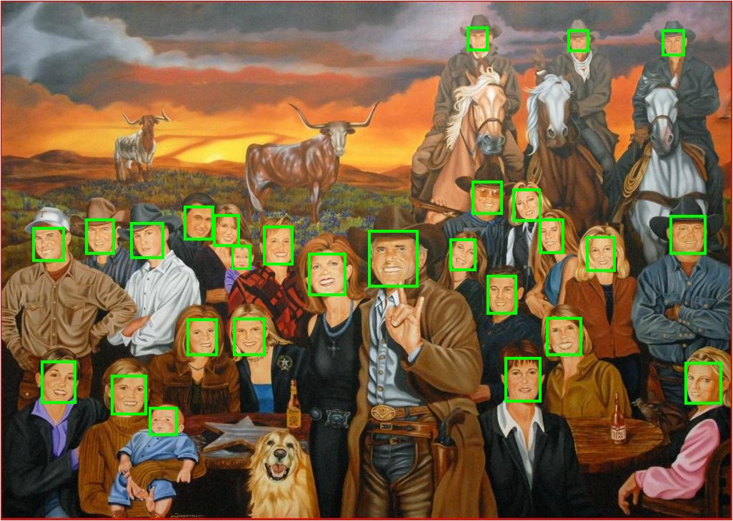
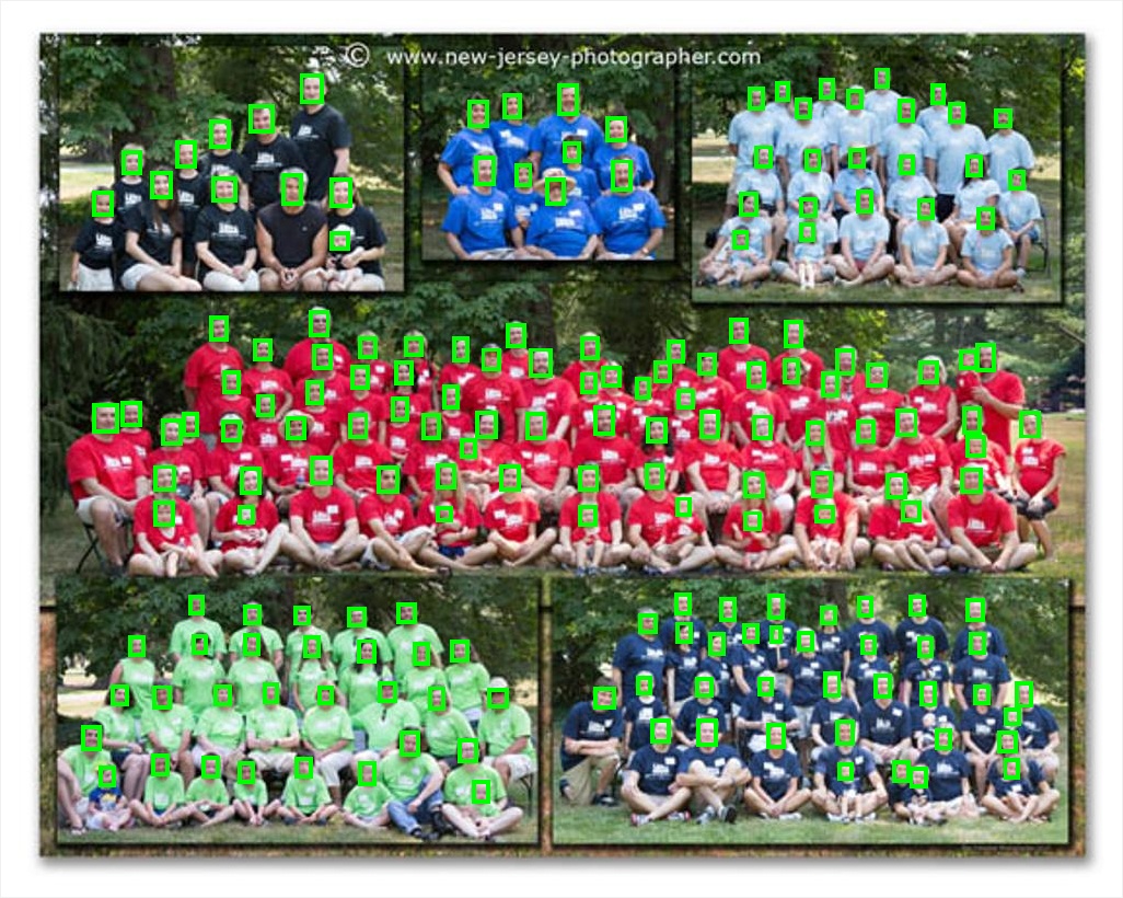
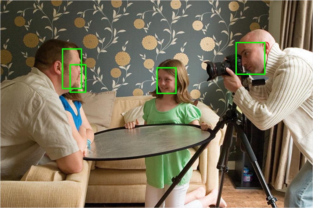
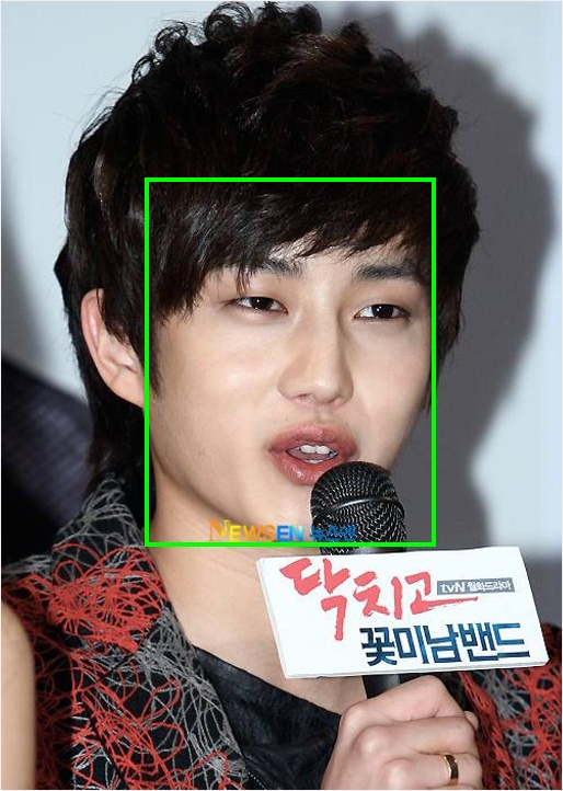
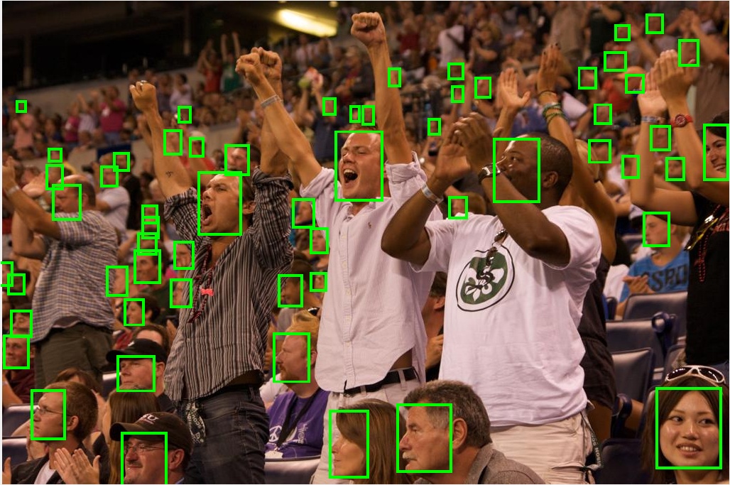
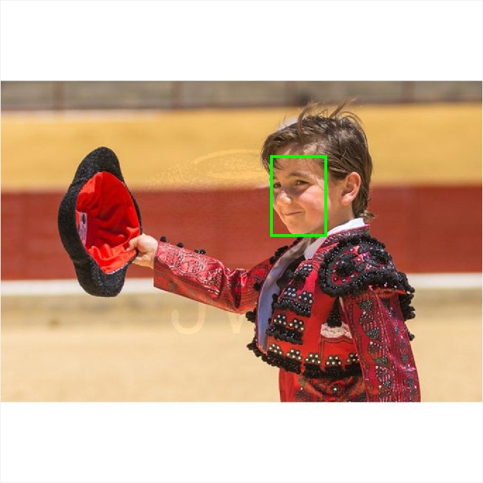
We train a Faster R-CNN face detection model on the recently released WIDER face dataset [16]. There are 12,880 images and 159,424 faces in the training set. In Fig. 1, we demonstrate some randomly sampled images of the WIDER dataset. We can see that there exist great variations in scale, pose, and the number of faces in each image, making this dataset challenging.

We train the face detection model based on a pre-trained ImageNet model, VGG16 [13]. We randomly sample one image per batch for training. In order to fit it in the GPU memory, it is resized based on the ratio $1024/\max(w,h)$, where $w$ and $h$ are the width and height of the image, respectively. We run the SGD solver 50k iterations with a base learning rate of 0.001 and run another 20K iterations reducing the base learning rate to 0.0001.

(a) 100 Proposals	(b) 300 Proposals
(c) 500 proposals	(d) 1000 proposals

Figure 2: Comparisons of face proposals on FDDB using different methods.

We test the trained face detection model on two benchmark datasets, FDDB [7] and IJB-A [8]. There are 10 splits in both FDDB and IJB-A. For testing, we resize the input image based on the ratio $\min(600/\min(w,h),1024/\max(w,h))$. For the RPN, we use only the top 300 face proposals to balance efficiency and accuracy.

For FDDB, we directly test the model trained on WIDER. For IJB-A, it is necessary to fine-tune the face detection model due to the different annotation styles between WIDER and IJB-A. In WIDER, the face annotations are specified tightly around the facial region while annotations in IJB-A include larger areas (e.g., hair). We fine-tune the face detection model on the training images of each split of IJB-A using only 10,000 iterations. In the first 5,000 iterations, the base learning rate is 0.001 and it is reduced to 0.0001 in the last 5,000. Note that there are more then 15,000 training images in each split. We run only 10,000 iterations of fine-tuning to adapt the regression branches of the Faster R-CNN model trained on WIDER to the annotation styles of IJB-A.

There are two criteria for quantatitive comparison for the FDDB benchmark. For the discrete scores, each detection is considered to be positive if its intersection-over-union (IoU) ratioe with its one-one matched ground-truth annotation is greater than 0.5. By varying the threshold of detection scores, we can generate a set of true positives and false positives and report the ROC curve. For the more restrictive continuous scores, the true positives are weighted by the IoU scores. On IJB-A, we use the discrete score setting and report the true positive rate based on the normalized false positive rate per image instead of the total number of false positives.

Figure 3: Comparisons of region-based CNN object detection methods for face detection on FDDB.

3.2 Comparison of Face Proposals

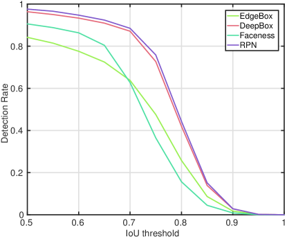
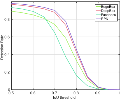
We compare the RPN with other approaches including EdgeBox [2], Faceness [15], and DeepBox [10] on FDDB. EdgeBox evaluates the objectness score of each proposal based on the distribution of edge responses within it in a sliding window fashion. Both Faceness and DeepBox re-rank other object proposals, e.g., EdgeBox. In Faceness, five CNNs are trained based on attribute annotations of facial parts including hair, eyes, nose, mouth, and beard. The Faceness score of each proposal is then computed based on the response maps of different networks. DeepBox, which is based on the Fast R-CNN framework, re-ranks each proposal based on the region-pooled features. We re-train a DeepBox model for face proposals on the WIDER training set.

(a)	(b)
(c)	(d)

Figure 4: Comparisons of face detection with state-of-the-art methods on (a) ROC curves on FDDB with discrete scores, (b) ROC curves on FDDB with discrete scores using less false positives, (c) ROC curves on FDDB with continuous scores, and (d) results on IJB-A dataset.

Figure 5: Sample detection results on the FDDB dataset, where green bounding boxes are ground-truth annotations and red bounding boxes are detection results of the Faster R-CNN.

Figure 6: Sample detection results on the IJB-A dataset, where green bounding boxes are ground-truth annotations and red bounding boxes are detection results of the Faster R-CNN.

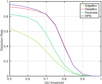
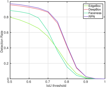
We follow [2] to measure the detection rate of the top $N$ proposals by varying the Intersection-over-Union (IoU) threshold. The larger the threshold is, the fewer the proposals that are considered to be true objects. Quantitative comparisons of proposals are displayed in Fig. 2. As can be seen, the RPN and DeepBox are significantly better than the other two. It is perhaps not surprising that learning-based approaches perform better than the heuristic one, EdgeBox. Although Faceness is also based on deeply trained convolutional networks (fine tuned from AlexNet), the rule to compute the faceness score of each proposal is hand-crafted in contrast to the end-to-end learning of the RPN and DeepBox. The RPN performs slightly better than DeepBox, perhaps since it uses a deeper CNN. Due to the sharing of convolutional layers between the RPN and the Fast R-CNN detector, the process time of the entire system is lower. Moreover, the RPN does not rely on other object proposal methods, e.g., EdgeBox.

3.3 Comparison of Region-based CNN Methods

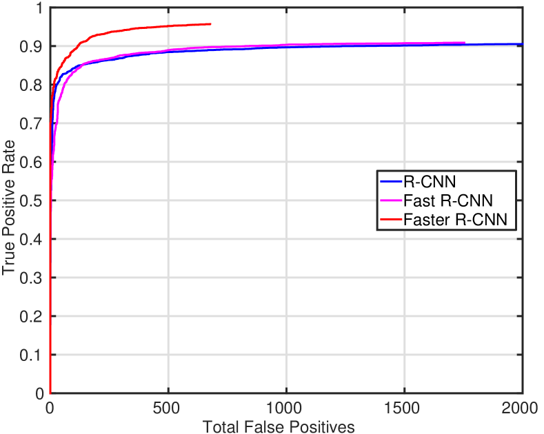
We also compare face detection performance of the R-CNN, the Fast R-CNN, and the Faster R-CNN on FDDB. For both the R-CNN and Fast R-CNN, we use the top 2000 proposals generated by the Faceness method [15]. For the R-CNN, we fine-tune the pre-trained VGG-M model. Different from the original R-CNN implementation [5], we train a CNN with both classification and regression branches end-to-end following [15]. For both the Fast R-CNN and Faster R-CNN, we fine-tune the pre-trained VGG16 model. As can be observed from Fig. 3, the Faster R-CNN significantly outperforms the other two. Since the Faster R-CNN also contains the Fast R-CNN detector module, the performance boost mostly comes from the RPN module, which is based on a deeply trained CNN. Note that the Faster R-CNN also runs much faster than both the R-CNN and Fast R-CNN, as summarized in Table 1.

3.4 Comparison with State-of-the-art Methods

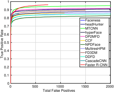
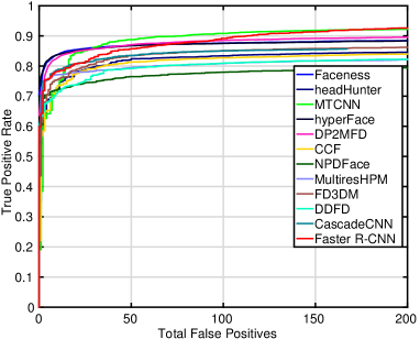
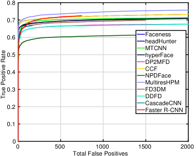
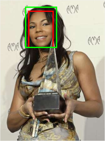
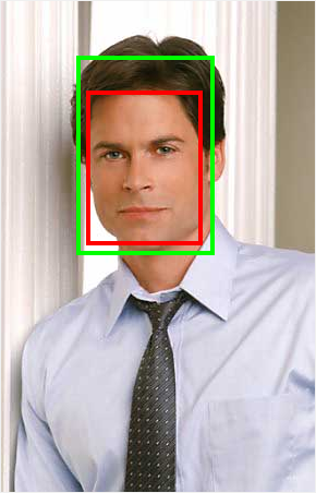
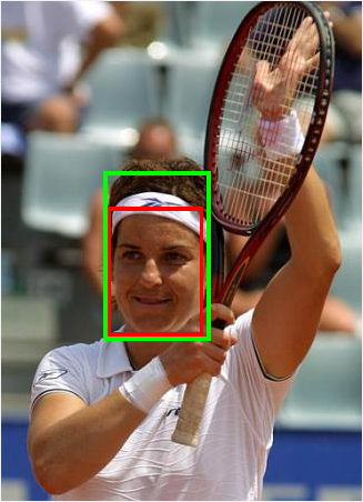
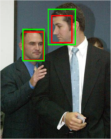
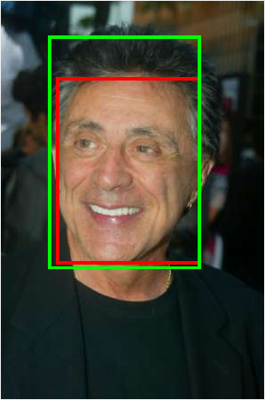
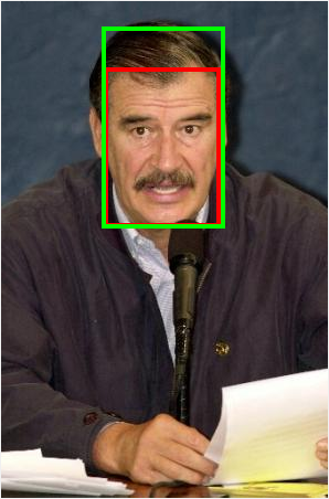
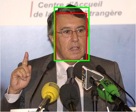
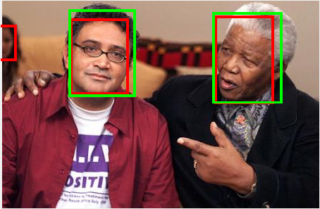
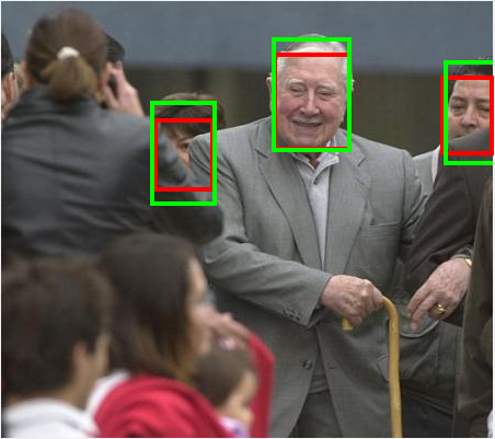
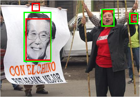
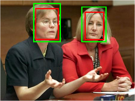
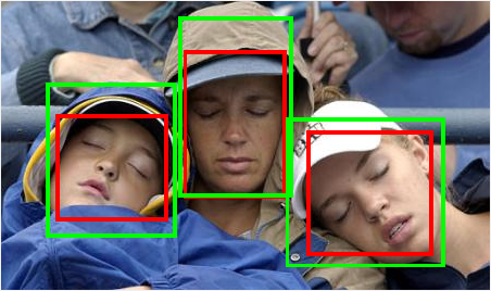
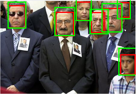
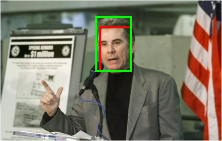
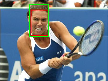
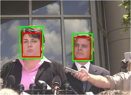
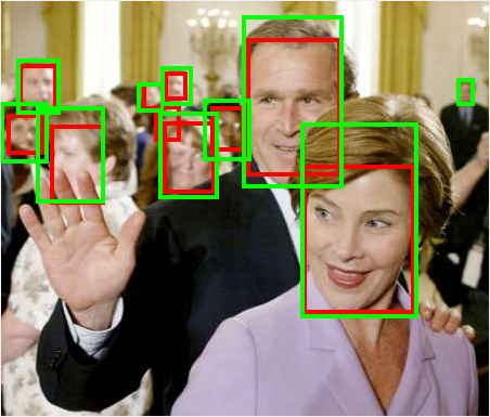
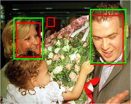
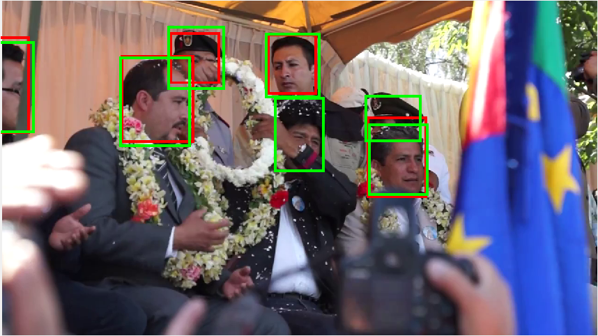
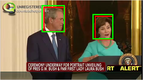
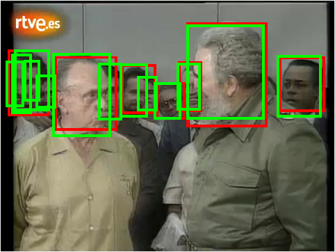
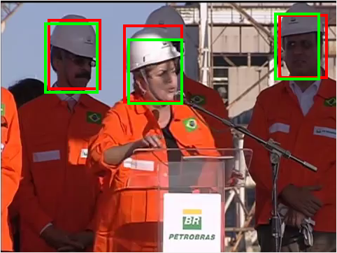
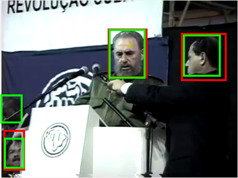
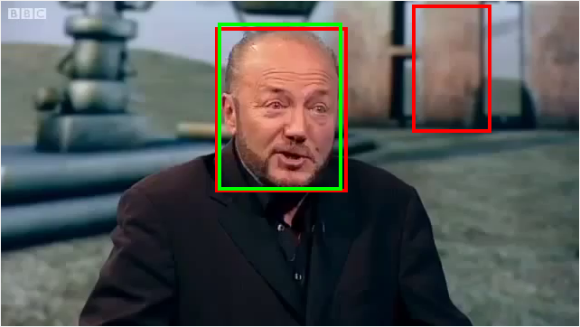
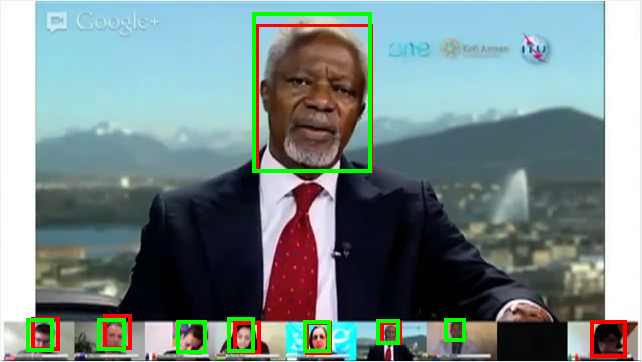
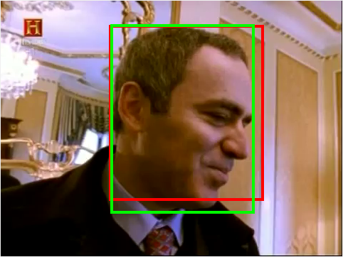
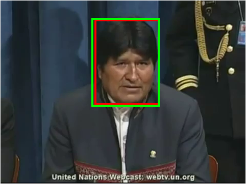
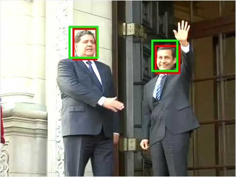
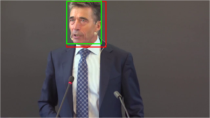
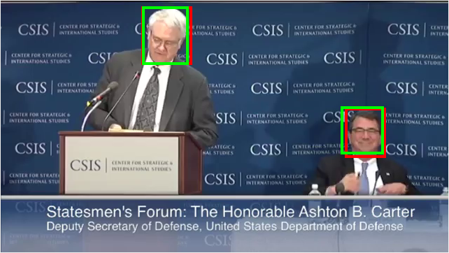
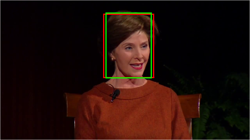
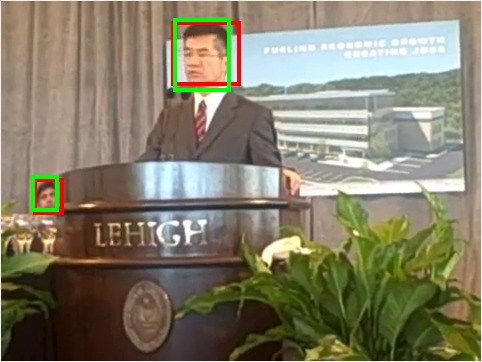
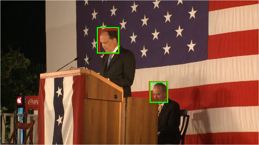
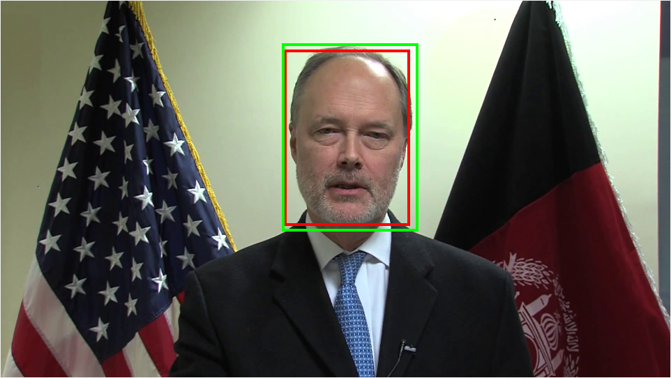
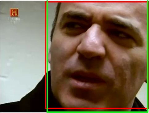
Finally, we compare the Faster R-CNN with 11 other top detectors on FDDB, all published since 2015. ROC curves of the different methods, obtained from the FDDB results page, are shown in Fig. 4. For discrete scores on FDDB, the Faster R-CNN performs better than all others when there are more than around 200 false positives for the entire test set, as shown in Fig. 4(a) and (b). With the more restrictive continuous scores, the Faster R-CNN is better than most of other state-of-the-art methods but poorer than MultiresHPM [3]. This discrepancy can be attributed to the fact that the detection results of the Faster R-CNN are not always exactly around the annotated face regions, as can be seen in Fig. 5. For 500 false positives, the true positive rates with discrete and continuous scores are 0.952 and 0.718 respectively. One possible reason for the relatively poor performance on the continuous scoring might be the difference of face annotations between WIDER and FDDB.

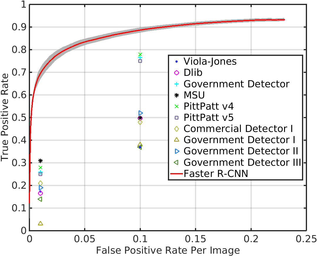
IJB-A is a relatively new face detection benchmark dataset published at CVPR 2015, and thus not too many results have been reported on it yet. We borrow results of other methods from [1, 8]. The comparison is shown in Fig. 4(d). As we can see, the Faster R-CNN performs better than all of the others by a large margin.

We further demonstrate qualitative face detection results in Fig. 5 and Fig. 6. It can be observed that the Faster R-CNN model can deal with challenging cases with multiple overlapping faces and faces with extreme poses and scales.

4 Conclusion

In this report, we have demonstrated state-of-the-art face detection performance on two benchmark datasets using the Faster R-CNN. Experimental results suggest that its effectiveness comes from the region proposal network (RPN) module. Due to the sharing of convolutional layers between the RPN and Fast R-CNN detector module, it is possible to use a deep CNN in RPN without extra computational burden.

Although the Faster R-CNN is designed for generic object detection, it demonstrates impressive face detection performance when retrained on a suitable face detection training set. It may be possible to further boost its performance by considering the special patterns of human faces.

References

- [1] J. Cheney, B. Klein, A. K. Jain, and B. F. Klare. Unconstrained face detection: State of the art baseline and challenges. In ICB, pages 229–236, 2015.
- [2] P. Dollár and C. L. Zitnick. Fast edge detection using structured forests. IEEE Trans. Pattern Anal. Mach. Intell., 37(8):1558–1570, 2015.
- [3] G. Ghiasi and C. C. Fowlkes. Occlusion coherence: Localizing occluded faces with a hierarchical deformable part model. In CVPR, pages 1899–1906, 2014.
- [4] R. B. Girshick. Fast R-CNN. In ICCV, pages 1440–1448, 2015.
- [5] R. B. Girshick, J. Donahue, T. Darrell, and J. Malik. Rich feature hierarchies for accurate object detection and semantic segmentation. In CVPR, pages 580–587, 2014.
- [6] K. He, X. Zhang, S. Ren, and J. Sun. Spatial pyramid pooling in deep convolutional networks for visual recognition. In ECCV, pages 346–361, 2014.
- [7] V. Jain and E. Learned-Miller. FDDB: A benchmark for face detection in unconstrained settings. Technical Report UM-CS-2010-009, University of Massachusetts, Amherst, 2010.
- [8] B. F. Klare, B. Klein, E. Taborsky, A. Blanton, J. Cheney, K. Allen, P. Grother, A. Mah, M. Burge, and A. K. Jain. Pushing the frontiers of unconstrained face detection and recognition: IARPA Janus benchmark A. In CVPR, pages 1931–1939, 2015.
- [9] A. Krizhevsky, I. Sutskever, and G. E. Hinton. Imagenet classification with deep convolutional neural networks. In NIPS, pages 1106–1114, 2012.
- [10] W. Kuo, B. Hariharan, and J. Malik. Deepbox: Learning objectness with convolutional networks. In ICCV, pages 2479–2487, 2015.
- [11] S. Ren, K. He, R. Girshick, and J. Sun. Faster R-CNN: Towards real-time object detection with region proposal networks. IEEE Trans. Pattern Anal. Mach. Intell., 2016.
- [12] S. Ren, K. He, R. B. Girshick, and J. Sun. Faster R-CNN: towards real-time object detection with region proposal networks. In NIPS, pages 91–99, 2015.
- [13] K. Simonyan and A. Zisserman. Very deep convolutional networks for large-scale image recognition. CoRR, abs/1409.1556, 2014.
- [14] J. R. R. Uijlings, K. E. A. van de Sande, T. Gevers, and A. W. M. Smeulders. Selective search for object recognition. International Journal of Computer Vision, 104(2):154–171, 2013.
- [15] S. Yang, P. Luo, C. C. Loy, and X. Tang. From facial parts responses to face detection: A deep learning approach. In ICCV, pages 3676–3684, 2015.
- [16] S. Yang, P. Luo, C. C. Loy, and X. Tang. WIDER FACE: A face detection benchmark. In CVPR, 2016.