Linear Perturbation Theory for Tidal Streams and the Small-scale CDM Power Spectrum

Abstract

Tidal streams in the Milky Way are sensitive probes of the population of low-mass dark–matter subhalos predicted in cold-dark-matter (CDM) simulations. We present a new calculus for computing the effect of subhalo fly-bys on cold streams based on the action–angle representation of streams. The heart of this calculus is a line-of-parallel-angle approach that calculates the perturbed distribution function of a stream segment by undoing the effect of all relevant impacts. This approach allows one to compute the perturbed stream density and track in any coordinate system in minutes for realizations of the subhalo distribution down to $10^{5}\,\mathrm{M}_{\odot}$, accounting for the stream’s internal dispersion and overlapping impacts. We study the statistical properties of density and track fluctuations with large suites of simulations of the effect of subhalo fly-bys. The one-dimensional density and track power spectra along the stream trace the subhalo mass function, with higher-mass subhalos producing power only on large scales, while lower mass subhalos cause structure on smaller scales. We also find significant density and track bispectra that are observationally accessible. We further demonstrate that different projections of the track all reflect the same pattern of perturbations, facilitating their observational measurement. We apply this formalism to data for the Pal 5 stream and make a first rigorous determination of $10^{+11}_{-6}$ dark–matter subhalos with masses between $10^{6.5}\,\mathrm{M}_{\odot}$ and $10^{9}\,\mathrm{M}_{\odot}$ within $20\,\mathrm{kpc}$ from the Galactic center (corresponding to $1.4^{+1.6}_{-0.9}$ times the number predicted by CDM-only simulations or to $f_{\mathrm{sub}}(r<20\,\mathrm{kpc})\approx 0.2\,\%$) assuming that the Pal 5 stream is $5\,\mathrm{Gyr}$ old. Improved data will allow measurements of the subhalo mass function down to $10^{5}\,\mathrm{M}_{\odot}$, thus definitively testing whether dark matter is clumpy on the smallest scales relevant for galaxy formation.

$\mathsection$ 1 Introduction

One of the fundamental predictions of the cold-dark-matter (CDM) cosmological model is that the halos of galaxies like the Milky Way should be filled with abundant substructure in the form of bound dark–matter subhalos. These subhalos are predicted to make up $\approx 10\,\%$ of the mass of the parent halo and to follow a mass spectrum that is approximately $\mathrm{d}n/\mathrm{d}M\propto M^{-2}$ (e.g., Klypin et al., 1999; Moore et al., 1999; Springel et al., 2008; Diemand et al., 2008) between the mass scale of the parent halo and the free-streaming scale (Schmid et al., 1999; Hofmann et al., 2001; Profumo et al., 2006). Yet this mass spectrum has so far eluded detection, except at the massive end where dark–matter subhalos are expected to host luminous satellite galaxies ($M\gtrsim 10^{8.5}\,\mathrm{M}_{\odot}$) (Strigari et al., 2008; Koposov et al., 2009) and where measurements of the small-scale power spectrum from the Lyman-$\alpha$ forest show the expected clustering ($M>3\times 10^{8}\,\mathrm{M}_{\odot}$; e.g., Viel et al. 2013). Whether or not dark matter clusters on smaller scales is a question that is of fundamental importance for the nature of dark matter. A clear detection of a CDM-like population of $M_{\mathrm{lim}}=3\times 10^{6}\,\mathrm{M}_{\odot}$ dark–matter subhalos would, for example, improve constraints on the mass $m_{\mathrm{WDM}}$ of the particle in thermal-relic warm dark matter models by a factor of $\approx 4$ to $m_{\mathrm{WDM}}\gtrsim 13$ keV as the lower limit scales as $m_{\mathrm{WDM}}>3.3\,\mathrm{keV}\,\left(3\times 10^{8}\,\mathrm{M}_{\odot}/M_{\mathrm{lim}}\right)^{0.3}$ following Viel et al. (2005, 2013).

Various techniques have been proposed to search for dark subhalos. In external galaxies, flux anomalies in strong gravitational lenses can reveal the presence of massive substructures (Mao & Schneider, 1998; Chiba, 2002; Dalal & Kochanek, 2002; Vegetti et al., 2012) and statistically probe the subhalo mass spectrum down to $\approx 10^{7}\,\mathrm{M}_{\odot}$ (Hezaveh et al., 2016). In our own galaxy, massive dark–matter clumps affect the structure of dynamically cold objects such as the disk (Lacey & Ostriker, 1985) and tidal streams (Johnston, 1998; Johnston et al., 2002; Ibata et al., 2002). The latter is the cleaner and more sensitive method, because of the number of other heating mechanisms that affect the structure and dynamics of the Galactic disk.

Early work on the interaction between dark–matter subhalos and tidal streams investigated the cumulative heating induced by the massive end of the subhalo mass spectrum using various $N$-body techniques (Johnston et al., 2002; Ibata et al., 2002; Carlberg, 2009). These papers predicted that the thin stellar streams formed by disrupting globular clusters would experience significant heating over a few Gyr and would therefore quickly disperse (Ibata et al., 2002; Carlberg, 2009). The very existence of long, thin tidal streams such as GD-1 (Grillmair & Dionatos, 2006) would therefore rule out a CDM-like population of dark subhalos. This strong effect is not seen in more recent simulations that contain a more realistic subhalo population (e.g., Yoon et al. 2011; Carlberg 2016) and long, narrow stellar streams appear compatible with a CDM-like subhalo population in a realistic halo (Ngan et al., 2016).

Recent work has focused on the density perturbations in tidal streams that are induced by the dynamical effect of subhalo fly-bys. Siegal-Gaskins & Valluri (2008) demonstrated with $N$-body simulations of a massive disrupting satellite in the presence of a CDM-like subhalo population that its tidal tails exhibit a large amount of clumpiness compared to simulations without subhalos. Much of the work in the past few years has specifically looked at gaps induced by subhalo fly-bys (e.g., Yoon et al. 2011; Carlberg 2012; Carlberg 2013; Erkal & Belokurov 2015a, Erkal & Belokurov 2015b) as the easiest detectable signal. Simplified dynamical modeling of increasing sophistication has elucidated the physical reason for gap formation due to subhalo encounters and allowed for analytic solutions for induced gap profiles and their evolution in time for circular orbits and in the absence of internal stream dispersion (Yoon et al., 2011; Carlberg, 2013; Erkal & Belokurov, 2015a). These methods have made it plausible that near-future measurements of the density and phase-space structure of streams will allow sensitive measurements of subhalo impacts down to at least $M\approx 10^{7}\,\mathrm{M}_{\odot}$ (Erkal & Belokurov, 2015b).

A number of cold streams have been found in the Milky Way’s stellar halo as overdensities of stars in color and magnitude (e.g., Pal 5; Odenkirchen et al. 2001; GD-1; Grillmair & Dionatos 2006; Grillmair 2009). However, despite improving measurements of their densities and increasingly sophisticated modeling of the effect of subhalo encounters, only vague statements regarding the consistency with the observed structure have been made so far (e.g., Yoon et al. 2011, Carlberg et al. 2012; Carlberg & Grillmair 2013; Carlberg 2016). While the level of density structure—often determined using the number of density gaps of a certain size—appears similar to that expected in CDM-like simulations, no clear measurement or constraint has been made so far. We believe that the problem is two-fold. Firstly, modeling the effect of subhalo impacts either assumes circular stream orbits and vanishingly small stream dispersion or uses expensive $N$-body modeling to run a small number of simulations. Thus, it has so far remained impossible to generate a large and realistic statistical sampling of the expected stream structure for a given model of the subhalo mass spectrum that could be compared with the data. Secondly, $N$-body simulations only very approximately return a model for an observed stream. Depending on the initial conditions and the perturbation history of the stream, the resulting stream today typically does not lie in the same location as where a stream is observed. Comparisons between the models and the data are therefore largely qualitative: no direct, rigorous comparison between the model and the data is possible.

In this paper we address both of these problems. Over the past few year, extensive progress has been made in modeling tidal streams (e.g., Eyre & Binney, 2011; Varghese et al., 2011; Bonaca et al., 2014; Bovy, 2014; Gibbons et al., 2014; Price-Whelan et al., 2014; Sanders, 2014; Amorisco, 2015; Bowden et al., 2015; Fardal et al., 2015; Küpper et al., 2015). Here, we specifically build on the advancements in modeling tidal stream in action–angle coordinates. While it has long been clear that action–angle coordinates provide the simplest description of the dynamics of tidal streams (Helmi & White, 1999; Tremaine, 1999), advances in computing the transformation between configuration space and action–angle space for realistic potentials to arbitrary accuracy in the last few years (Bovy, 2014; Sanders & Binney, 2014; Binney & McMillan, 2016) has made action–angle modeling of tidal streams practical. In particular, Bovy (2014) and Sanders (2014) have demonstrated that the structure of unperturbed tidal streams—disrupting clusters or low-mass dwarf galaxies in a smooth background potential—can be accurately and efficiently modeled using simple prescriptions in the space of orbital frequencies and angles. Sanders et al. (2016) recently showed that this modeling framework can be extended to model the effect of a single dark–matter impact on a stellar stream: the impulsive velocity kicks from the impact can be transformed to frequency–angle space where they produce a instantaneous change in the frequencies and angles of all stream stars that gets added to their otherwise linear frequency–angle dynamics.

Here, we extend this approach into a new calculus for computing the present-day structure of a tidal stream perturbed by many dark–matter subhalo encounters. As in Sanders et al. (2016), we employ simple models for the distribution of stars in the unperturbed stream and combine it with impulsive kicks transformed to frequency–angle space. We demonstrate how we can then compute the present-day stream structure to high accuracy in the linear regime where all kicks are calculated based on the location of the stream in the absence of impacts. However, we apply the kicks to the perturbed streams and take the dispersion in the stream and the overlapping effects of multiple impacts into account. We test that this linear perturbation theory applies using a set of $N$-body simulations that include the full non-linear interactions. In the linear regime, we then develop a new “line-of-parallel-angle” algorithm for the fast computation of the present-day stream structure by efficiently undoing the effect of all impacts that affect a given position along the stream. Like in Sanders et al. (2016), these simulations can be tailor-made to an observed tidal stream, returning predictions that may be directly and quantitatively compared to observed streams.

We use this fast and accurate algorithm to run a large suite of simulations of the effect of subhalo impacts on cold stellar streams. Rather than looking for gaps of different sizes, we directly consider the power spectrum of density fluctuations and demonstrate that the effect of a given subhalo mass range leaves a clear imprint on a specific scale that can be used to robustly infer the number of subhalos in different mass ranges down to $M=10^{5}\,\mathrm{M}_{\odot}$. We also investigate power spectra of fluctuations in the position and velocity of the stream track, cross power spectra of track and density fluctuations, and bispectra of the density and track. All of these are within reach of observations that will occur in the next decade and a detection in multiple of these channels would constitute a clear proof that the observed stream structure is due to low-mass dark–matter subhalos.

In total, the results in this paper are based on $\approx 500,000$ simulations of subhalo impacts on tidal streams, many with hundreds of impacts per realization. This can be compared to the number of realizations performed in state-of-the-art $N$-body simulations of subhalo–stream interactions, which only number in the hundreds (Carlberg, 2016). The statistical sampling that is opened up by our fast method clarifies many of the effects that are normally buried within the realization-to-realization scatter.

To aid the reader in navigating this long paper, we provide a brief overview of all sections here. Section 2 contains generalities about the manner in which we model tidal streams in frequency–angle space ($\mathsection$ 2.1), how we apply subhalo kicks in this space ($\mathsection$ 2.2), and how we sample the number of impacts and the fly-by parameters ($\mathsection$ 2.3). Section 3 discusses various methods for evaluating the phase–space structure of tidal streams perturbed by a large number of subhalo impacts: $\mathsection$ 3.1 describes how to do this by Monte Carlo simulations of tracer particles in the perturbed stream and $\mathsection$ 3.2 gives a general method for evaluating the phase–space distribution function of a perturbed stream analytically. Section 3.3 presents the fast line-of-parallel-angle method for evaluating the phase–space distribution function and its moments that allows for the full density and phase–space structure of a perturbed stream to be computed in minutes. The last subsection of Section 3, $\mathsection$ 3.4, discusses how to convert the computed structure in frequency–angle space to configuration space, where it can more easily be compared to observations. Section 4 employs this fast method to investigate the density and track power spectra of tidal streams perturbed by a variety of subhalo populations. Section 5 goes beyond the power spectrum and demonstrates that perturbed tidal streams also have significant bispectra, that is, third order moments. We discuss the power spectra and bispectra in configuration space (as opposed to frequency–angle space as in $\mathsection$$\mathsection$ 4 and 5) in Section 6. We apply our formalism to density data for the Pal 5 stream in $\mathsection$ 7 and perform a first measurement of the number of subhalos in the inner Milky Way based on this data. Section 8 discusses various aspects of the work presented here and we conclude with some final remarks in $\mathsection$ 9.

A collection of appendices contains various further technical aspects of our work. Appendix A describes a suite of tests of our formalism using full $N$-body simulations of the interaction between dark–matter subhalos and tidal streams. Appendix B holds a detailed derivation of the fast line-of-parallel angle algorithm presented in $\mathsection$ 3.3 for the case of multiple impacts. Various convergence tests for the power spectra from $\mathsection$ 4 are presented in Appendix C. Finally, Appendix D tests our analysis of the Pal 5 data by repeating it for a few $N$-body simulations of the Pal 5 stream perturbed by varying levels of substructure. All calculations in this paper make heavy use of the galpy galactic dynamics code (Bovy, 2015) (see $\mathsection$ 9 for full details on code availability).

$\mathsection$ 2 Stream and impact modeling

Figure 1: Properties of the mock GD-1-like stream used throughout this paper. The top panel displays the position on the sky of the leading arm (the trailing arm is not used here), the middle panel gives the relation between the Galactic longitude and the parallel angle along the stream, and the bottom panel gives the density of the stream. All of these properties are for the smooth, unperturbed stream. The position of the progenitor cluster is indicated with a black dot in the top two panels. The dashed line is the location of the end of the stream for the purposes of this paper.

2.1 Smooth stream model

In this paper, we employ a mock stellar stream similar to that used by Bovy (2014) to investigate the effect of multiple dark-matter-halo impacts on tidal streams. In particular, we make use of the simple model in frequency–angle space from Bovy (2014) as the basis of all our calculations of the effect of impacts. The model stream in frequency–angle space that we use to illustrate our computations is the same as that from sections 3.2 and 3.3 of Bovy (2014), except that we make the stream twice as old ($9\,\mathrm{Gyr}$ vs. $4.5\,\mathrm{Gyr}$) and twice as cold (a model velocity dispersion $\sigma_{v}=0.1825\,\mathrm{km\ s}^{-1}$ rather than $\sigma_{v}=0.365\,\mathrm{km\ s}^{-1}$) to create a stellar stream that is older, but has the same length as the stream from Bovy (2014). The current progenitor position and past orbit in a flattened logarithmic potential with a circular velocity of $220\,\mathrm{km\ s}^{-1}$ and a potential flattening of $q=0.9$ are kept the same and the resulting stream resembles the GD-1 stream (Grillmair & Dionatos, 2006; Koposov et al., 2010). The progenitor’s orbit has a pericenter of $13.7\,\mathrm{kpc}$, an eccentricity of $0.31$, and is close to pericenter at the current time ($r=14.4\,\mathrm{kpc}$). The radial period is approximately $400\,\mathrm{Myr}$. The details of the Milky-Way-like potential are unimportant for the forecasting that we perform using the GD-1-like stream as long as it realistically describes the divergence of nearby orbits due to kicks from dark-matter-halo fly-bys, which this flattened potential does.

The model of Bovy (2014)—as well as the similar one of Sanders (2014)—fundamentally lives in frequency–angle space. Briefly, based on a model host potential, current progenitor position, velocity-dispersion parameter $\sigma_{v}$, and a time $t_{d}$ at which disruption started, a model for the leading or trailing tail of the stream is created in frequency–angle space as follows. The properties of the progenitor orbit are employed to create an approximate Gaussian action $\mathbf{J}$ distribution for the tidal debris (Eyre & Binney, 2011), which is then transformed to frequency $\mathbf{\Omega}$ space using the Hessian $\partial\mathbf{\Omega}/\partial\mathbf{J}$ evaluated at the progenitor’s actions. The principal eigenvector of the resulting variance tensor in frequency space is the parallel-frequency direction, that is, the direction in frequency space along which the stream spreads. The eigenvalues of the eigenvectors perpendicular to the parallel frequency are typically a factor of 30 or more smaller than the largest eigenvalue (Sanders & Binney, 2013). The dispersion of the debris in frequency space is scaled by the velocity-dispersion parameter $\sigma_{v}$ and the relative eigenvalues; the full frequency distribution is modeled as a Gaussian with a mean that is offset from the progenitor’s frequency and the variance tensor resulting from propagating the Gaussian action distribution to frequency space, multiplied by the magnitude of the parallel frequency (the latter because this simplifies analytical calculations). For the purposes of this paper, the initial spread in angle of the tidal debris is zero. After debris is tidally stripped from the progenitor with the frequency distribution given above, it evolves in the host potential only and the future location at all times can be computed from the linear evolution in angle space, with the frequency remaining constant. In angle space, the stream spreads primarily in the direction parallel to the parallel-frequency direction and the angle offset from the progenitor in this direction is denoted as $\Delta\theta_{\parallel}$; the corresponding parallel frequency is denoted $\Delta\Omega_{\parallel}$. Debris is generated with a distribution of stripping times, assumed constant up to a maximum time $t_{d}$—the time since disruption commenced—in the simplest model. As discussed below, none of the specific assumptions of (close-to) Gaussian frequency distribution or uniform stripping rate is crucial to the fast method presented below for computing the effect of impacts.

As discussed by Bovy (2014), the above analytic model in frequency–angle space can be efficiently transformed to configuration space by linearizing the transformation between configuration space and frequency–angle space near the track of the stream. Starting from the progenitor orbit, the mean path of the stream in configuration space can be iteratively computed starting from the progenitor’s orbit, with convergence typically attained after one iteration. This generates a continuous model for the phase-space structure of a stellar stream (as opposed to discrete, $N$-body models) and in particular, a smooth, continuous representation of the stream track—the average phase-space location as a function of distance from the progenitor. In this paper, this allows us to transform determinations of the stream structure due to dark–matter-halo impacts from frequency–angle space—where they are most easily computed—to configuration space.

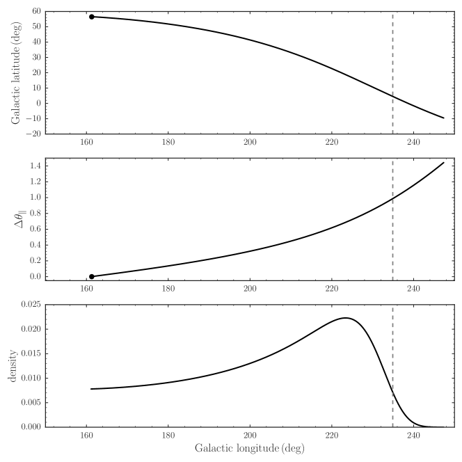
The model of Bovy (2014) and the computation of the effects of impacts on a stellar stream below both consider the leading and trailing arms of a stream separately. Therefore—and because it creates a long stream on its own—we only consider the leading arm of the stream. For the purpose of modeling dark-matter-halo kicks, whether a tail is leading or trailing does not matter greatly, because the high surface-brightness part of a tidal tail has approximately constant actions (Bovy, 2014). Some of the properties of the leading arm (without perturbations due to dark–matter-halo impacts) are displayed in Figure 1; other projections of the current phase–space position are similar to those in Figs. 7 and 8 of Bovy (2014). The top panel demonstrates the path on the celestial sphere traced by the smooth stream. The leading arm spans approximately $93^{\circ}$ on the sky, has a physical length of $\approx 12.4\,\mathrm{kpc}$, and an angular Gaussian width of $\approx 14^{\prime}$, similar to the GD-1 stream (Koposov et al., 2010; Carlberg & Grillmair, 2013). The middle panel shows the relation between Galactic longitude $l$ and the parallel angle $\Delta\theta_{\parallel}$. Most of the calculations in this paper are performed as a function of parallel angle $\Delta\theta_{\parallel}$ and we will discuss the structure of the stream induced by impacts as a function of this angle. The middle panel demonstrates that $\Delta\theta_{\parallel}$ is a smooth transformation of the observable coordinate along the stream, in this case Galactic longitude. The bottom panel of Figure 1 displays the density of the smooth stream, computed analytically from the smooth stream model. The mock stream has a smooth, close-to-constant density profile all the way until the edge of the stream, defined here as the location along the stream where the density (as a function of $\Delta\theta_{\parallel}$, not longitude) drops below $20\,\%$ of that near the progenitor; this location is indicated by the dashed vertical line. We use the density as a function of $\Delta\theta_{\parallel}$ because this is easy to compute and it returns a length that increases linearly with time; we demonstrate in Appendix C that the exact definition of the length is unimportant for predicting the statistical structure of perturbed streams. The density enhancement around $l\approx 220^{\circ}$ is due to a factor of two variation in the Jacobian of the transformation between $\Delta\theta_{\parallel}$ and $l$ in the smooth logarithmic potential.

Figure 2: Relative probability of impacts at different times in the past ($t_{\mathrm{impact}}$) for the GD-1-like stream from Figure 1. The relative probability is proportional to the length of the stream in configuration space at different times and normalized such that it integrates to one. The oscillations are due to the eccentric nature of the progenitor orbit, with the stream being longer near pericentric passages and shorter near apocentric passages. The radial period for the progenitor cluster is $\approx 400\,\mathrm{Myr}$.

2.2 Angle–frequency perturbations due to subhalo impacts

Sanders et al. (2016) demonstrated that the interaction between a stellar stream and a dark–matter halo can be efficiently modeled in frequency–angle space by transforming the impulsive kicks resulting from this interaction to frequency–angle space. Because this formalism forms the basis of the calculations in this paper, we briefly review its main ingredients here.

A dark–matter halo having a close encounter with a stellar stream imparts a perturbation to the orbits of stars in the stream that can be accurately computed in the impulse approximation (Yoon et al., 2011; Carlberg, 2013; Erkal & Belokurov, 2015a). Thus, the effect of the dark–matter halo is approximated as resulting in an instantaneous velocity kick $\delta\mathbf{v}^{g}$ imparted at the time of closest approach between the dark–matter halo and the stream. This velocity kick $\delta\mathbf{v}^{g}$ can be transformed to frequency–angle space using the Jacobians $\partial\mathbf{\Omega}/\partial\mathbf{v}$ and $\partial\boldsymbol{\theta}/\partial\mathbf{v}$, resulting in frequency and angle kicks $\delta\mathbf{\Omega}^{g}$ and $\delta\boldsymbol{\theta}^{g}$. Before the impact, a star with coordinates $(\mathbf{\Omega},\boldsymbol{\theta})$ has the equation of motion $\mathbf{\Omega}=\mathbf{\Omega}_{0}=$ constant, $\boldsymbol{\theta}=\mathbf{\Omega}_{0}\,t+\boldsymbol{\theta}_{0}$, with $(\mathbf{\Omega}_{0},+\boldsymbol{\theta}_{0})$ the initial frequency–angle position at the time of stripping. After the impact at time $t^{g}$, this star has the equation of motion $\mathbf{\Omega}=\mathbf{\Omega}_{0}+\delta\mathbf{\Omega}^{g}=$ constant, $\boldsymbol{\theta}=\mathbf{\Omega}_{0}\,t+\delta\mathbf{\Omega}^{g}\,(t-t^{g})+\delta\boldsymbol{\theta}^{g}+\boldsymbol{\theta}_{0}$. As in Sanders et al. (2016), we will assume that observations happen at $t=0$ and specify impact times as happening $t_{i}$ in the past (i.e., $t_{i}$ is positive for an impact in the past and is zero for the current time).

Sanders et al. (2016) demonstrated that the following approximate form of the above formalism accurately models the effect of a dark–matter halo fly-by at all times in the future and in both frequency–angle and configuration space. Rather than computing the kicks $\delta\mathbf{v}^{g}$ over the full six-dimensional phase–space volume of the stream, we can compute it for the mean stream track $(\mathbf{x},\mathbf{v})(\Delta\theta_{\parallel})$ and apply the kicks based on the nearest $\Delta\theta_{\parallel}$ to any phase–space location populated by the stream. That is, we only need to compute $\delta\mathbf{v}^{g}$—and the resulting $\delta\mathbf{\Omega}^{g}$ and $\delta\boldsymbol{\theta}^{g}$—along the one-dimensional mean locus of the stream at the time of impact (which can be efficiently computed for the Bovy (2014) stream model as discussed above). Furthermore, Sanders et al. (2016) showed that the angle kicks $\delta\boldsymbol{\theta}^{g}$ are small compared to the frequency kicks $\delta\mathbf{\Omega}^{g}$ after approximately one period. Because the orbital periods of old, long stellar streams are much shorter than their age, we therefore ignore the angle kicks in the calculations in this paper. These approximations are extensively tested in the following sections and in Appendix A.

2.3 Statistical sampling of multiple impacts

If the Milky Way’s halo is populated by a population of dark–matter halos orbiting within it, tidal streams are expected to have interactions with multiple halos over their lifetimes. In this section, we describe how we sample the distribution of possible impacts to generate a realization of a tidal stream perturbed by multiple encounters. In the model of Sanders et al. (2016) summarized above, for a given underlying smooth stream model, a single impact is fully described by (a) the time $t_{i}$ at which the impact occurs, (b) the angular offset $\Delta\theta_{\parallel}^{i}$ from the progenitor of the closest approach between the dark–matter halo and the stellar stream, (c) the fly-by velocity $\mathbf{w}$ of the dark–matter halo, (d) the mass $M$ and internal structure of the perturber (specified using a single scale parameter $r_{s}$), and (e) the impact parameter $b$. We sample the parameters in this order, i.e., later parameters in this sequence are sampled conditional on the value sampled earlier in the sequence.

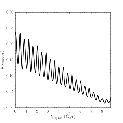
We sample impact times from a distribution $p(t_{i})$ that corresponds to the relative length of the stream at different times. That is, the probability that the stream is hit at time $t_{i}$ is proportional to the physical length of the stream at that time. In practice, we compute the length of the stream as the path length in position space between the progenitor and the point along the stream where the density as a function of $\Delta\theta_{\parallel}$ drops below 20 % (see $\mathsection$ 2.1). The probability distribution $p(t_{i})$ computed in this way is shown in Figure 2. The probability $p(t_{i})$ displays a general increase toward more recent times (smaller $t_{i}$), because of the increasing length of the stream, but it also takes into account the relative shortening and lengthening of the stream near apo- and pericenter. The latter gives rise to the oscillatory behavior in Figure 2.

To sample the angular offset $\Delta\theta_{\parallel}^{i}$ of the closest approach for a given $t_{i}$, we similarly compute the relative physical lengths of different parts of the stream at $t_{i}$ and sample $\Delta\theta_{\parallel}^{i}$ proportional to this (in practice we do this by discretizing the stream at each time using $\approx 1000$ segments). This $t_{i}$ sampling assumes that the subhalo population does not evolve over time. The subhalo population is expected to change as the accretion rate of subhalos varies with time or because of mass-loss from tidal stripping (Diemand et al., 2007). In the inner Milky Way, subhalos may also get depleted through their interaction with the Milky Way’s disk (D’Onghia et al., 2010), in which case the incidence of substructure is higher at earlier times. The $p(t_{i})$ distribution computed based on the relative length of the stream could be multiplied by a function to account for the time evolution of the number of subhalos to account for these effects.

As discussed by Erkal et al. (2016) (see also Carlberg 2012), for a Gaussian distribution of velocities of the population of dark–matter halos characterized by a velocity dispersion $\sigma_{h}$, the distribution of velocities $\mathbf{w}$ that enter a cylinder around the stream is as follows. In the cylindrical coordinate frame centered on the position of the stream at the point of closest approach (specified by $\Delta\theta_{\parallel}^{i}$), with the $z$ axis pointing along the stream, and at rest with respect to the Galactic center (thus, not co-moving with the stream), the $z$ and tangential velocities are normally distributed with dispersion $\sigma_{h}$, while the negative radial velocity $w_{r}$ has a Rayleigh distribution with the same dispersion (positive radial velocities have zero probability, because these move away from the stream): $p(w_{r})=|w_{r}|/\sigma_{h}^{2}\,\exp\left(-w_{r}^{2}/[2\,\sigma_{h}^{2}]\right)$. In the impulse approximation, the velocity at closest approach is the same as when the dark–matter subhalo enters this “cylinder-of-influence”. Therefore, we sample the fly-by velocity in the cylindrical frame from these distributions and rotate it to the Galactocentric frame using our knowledge of the stream track at the time of impact.

The mass $M$ and internal profile of the dark–matter perturber and the impact parameter are sampled last. In this paper, we specify the internal profile in terms of a scale radius $r_{s}$ parameter and we consider both Hernquist and Plummer profiles for the perturbers. Thus, the internal profile is sampled by drawing $r_{s}$ values. As discussed by Erkal et al. (2016) (see also Yoon et al. 2011; Carlberg 2013), the impact parameter $b$ for a subhalo entering the roughly cylindrical volume of a stellar stream is uniformly distributed. We thus sample $b$ from a uniform distribution between $-b_{\mathrm{max}}$ and $b_{\mathrm{max}}$. Smaller, lower-mass dark–matter halos need to pass more closely to a stellar stream to have an observable effect. Below, we find that setting $b_{\mathrm{max}}$ equal to a multiple $X$ of the scale radius of the dark–matter halo works well to take the decreasing volume of the interaction with decreasing mass into account. Therefore, we need to sample $M$ and $r_{s}$ of the dark–matter halo first, from the marginalized distribution $p(M,r_{s})=\int\mathrm{d}b\,p(M,r_{s},b)$. We further make use of a deterministic $r_{s}(M)$ relation (i.e., we assume that the scale radius is exactly specified by the mass) of the form $r_{s}\propto M^{0.5}$ (Diemand et al., 2008). Then, if the population of dark–matter halos has a spectrum $\mathrm{d}n/\mathrm{d}M$, we sample $M$ from a distribution $\propto M^{0.5}\,\mathrm{d}n/\mathrm{d}M$. We use a fiducial $\mathrm{d}n/\mathrm{d}M\propto M^{-2}$, for which $p(M)\propto M^{-1.5}$. After sampling $M$ in this way, we determine $r_{s}$ and sample $b$ uniformly between $-Xr_{s}$ and $Xr_{s}$. Our fiducial dark–matter subhalo model is that of a Hernquist sphere with $r_{s}(M)=1.05\,\mathrm{kpc}\,\left(M/10^{8}\,\mathrm{M}_{\odot}\right)^{0.5}$, obtained by fitting Hernquist profiles to the circular-velocity–mass relation in the Via Lactea II simulation (Diemand et al., 2008).

Finally, we need to sample the number of impacts from a Poisson distribution for the expected number of impacts. We refer to this interchangeably as the “expected number” or as the “rate” below; the rate is always per stream age. For this we follow Yoon et al. (2011) in writing the number of impacts in an interval $\mathrm{d}t$ and integrate that over the lifetime of the stream, but using the modified formalism of Erkal et al. (2016), that uses the correct distribution of fly-by velocities (see above). We could use the same approach as in Figure 2 to compute the length of the stream at all times, but for simplicity we approximate the stream as increasing its length linearly in time as $\Delta\Omega^{m}$, where $\Delta\Omega^{m}$ is the mean-parallel-frequency parameter of the smooth stream (see Bovy 2014). The expression for the expected number of impacts for either the leading or trailing arm is then

$$N_{\mathrm{enc}}=\sqrt{\frac{\pi}{2}}\,r_{\mathrm{avg}}\,\sigma_{h}\,t_{d}^{2}\,\Delta\Omega^{m}\,b_{\mathrm{max}}\,n_{h}\,,$$ (1)

where $r_{\mathrm{avg}}$ is the average spherical radius of the stream and $n_{h}$ is the number density of dark–matter halos in the mass range considered. For the GD-1-like stream, this rate is approximately 62.7 when considering impacts between $10^{5}\,\mathrm{M}_{\odot}$ and $10^{9}\,\mathrm{M}_{\odot}$ out to $b_{\mathrm{max}}=5\,r_{s}(M)$ for $n_{h}$ corresponding to 425.79 dark–matter subhalos in this mass range within $25\,\mathrm{kpc}$ from the Galactic center. The latter number is obtained by considering 38.35 subhalos within $25\,\mathrm{kpc}$ from the Galactic center with masses between $10^{6}\,\mathrm{M}_{\odot}$ and $10^{7}\,\mathrm{M}_{\odot}$ and scaling this number by a factor of ten more or less for each higher or lower mass decade ($\mathrm{d}n/\mathrm{d}\log_{10}M\propto M^{-1}$; similar to the numbers obtained from the Via Lactea II simulation by Yoon et al. 2011).

$\mathsection$ 3 The phase–space structure of a perturbed stream

In this section, we discuss methods for evaluating the phase–space structure of perturbed tidal streams. Our modeling approach is that of a generative model for a tidal stream in frequency–angle space. This model has two main ingredients: (a) the prescription for how stars are released from the progenitor cluster or satellite and how they orbit in the smooth background potential and (b) the set of dark-matter–halo kicks that perturbs the orbits of stream stars. Ingredient (a) on its own produces the smooth stream and we use the model of Bovy (2014) (see $\mathsection$ 2.1 above). Part (b) applies the perturbations from subhalo impacts.

For a given set of subhalo perturbations, a star in a tidal stream with a given initial phase–space position has a deterministic path that leads to its observed position today. Because of the conservation of phase–space volume, the phase–space distribution function $p(\mathbf{\Omega},\boldsymbol{\theta})$ of tidal debris today at a point $(\mathbf{\Omega},\boldsymbol{\theta})$ ago is therefore equal to the distribution of the debris just after release (assuming that $|\partial\mathbf{\Omega}/\partial\mathbf{J}|$ does not vary substantially, which is a good assumption for a cold stellar stream). Therefore, evaluating the phase–space structure of a perturbed stream can be performed in two ways. We can start from the distribution of debris at the time that it is stripped and apply perturbations while evolving the debris forward to arrive at the present-day distribution of debris. A simple implementation of this is to generate mock perturbed–stream data. We start by describing this in $\mathsection$ 3.1, because this is the simplest manner in which to determine the perturbed structure of a stream. While straightforward, it is difficult to compute the phase–space distribution at a given current location in this manner, because one does not know where one will end up when starting at an initial debris location.

Figure 3: Flowchart for the direct determination of $p(\Delta\Omega_{\parallel},\Delta\theta_{\parallel})$ by undoing the effect of all impacts up to the time of stripping. This procedure is illustrated graphically in Figure 4. In this flowchart, $t_{i}^{0}=0$.

To evaluate the phase–space distribution at a given $(\mathbf{\Omega},\boldsymbol{\theta})$, we need to specify the time at which this point was stripped (a time $t_{s}$ in the past) and to run the stream backward in time while undoing the effect of all impacts. Then we arrive at the initial $(\mathbf{\Omega}_{0},\boldsymbol{\theta}_{0})$ a time $t_{s}$ in the past. We can then evaluate the probability distribution for the initial distribution of the debris $p_{0}(\mathbf{\Omega}_{0},\boldsymbol{\theta}_{0},t_{s})$. This backward-evolution method allows for faster and more accurate ways of computing the perturbed stream structure today. Various forms of the backward-evolution method are described in $\mathsection$$\mathsection$ 3.2 and 3.3.

Readers uninterested in the details of how we compute the perturbed structure of tidal streams can safely skip ahead to $\mathsection$$\mathsection$ 4 and beyond, which do not require a detailed understanding of the calculation.

3.1 Sampling mock perturbed–stream data

To sample mock data, we start with the model of the smooth stream, which provides a model for the orbits (given by $\Delta\mathbf{\Omega}$ relative to the progenitor) onto which stars are released from the progenitor at different times $t_{s}$ in the past. We denote this model by the probability distribution $p_{0}(\Delta\mathbf{\Omega},t_{s})$. In the simple model of Bovy (2014) described in $\mathsection$ 2.1, this model has a uniform distribution of $t_{s}$ up to a time $t_{d}$—which defines the start of tidal disruption—and a stationary distribution of $\Delta\mathbf{\Omega}$: $p_{0}(\Delta\mathbf{\Omega},t_{s})\propto p_{0}(\Delta\mathbf{\Omega})$ for $t_{s}<t_{d}$. We sample $\Delta\mathbf{\Omega}$ and $t_{s}$ from this model to generate the leading or trailing arm of a tidal stream.

For a given mock star $(\Delta\mathbf{\Omega},t_{s})$, we compute the parallel angle this star reaches at the first impact that occurs after it was stripped ($\Delta\theta_{\parallel}=\Delta\Omega_{\parallel}\times\max_{k;t_{i}^{k}<t_{s}}t^{k}_{i}$, for impacts $k$ at times $t_{i}^{k}$). We add the kick $\delta\mathbf{\Omega}^{g,k}$ at this $\Delta\theta_{\parallel}$ to $\Delta\mathbf{\Omega}$ and similarly add the kick $\delta\boldsymbol{\theta}^{g,k}$ to $\Delta\boldsymbol{\theta}$. We then repeat this procedure for each subsequent impact. After the final (most recent) impact, the star reaches its present $(\Delta\mathbf{\Omega},\Delta\boldsymbol{\theta})$. At this point, we can use the linearized frequency–angle transformation in the vicinity of the stream to compute the configuration-space coordinates of this point: $(\Delta\mathbf{\Omega},\Delta\boldsymbol{\theta})\rightarrow(\mathbf{x},\mathbf{v})$.

This procedure is very simple to apply, but becomes quite computationally expensive when many impacts are involved (streams have $\mathcal{O}(100)$ impacts when considering dark–matter subhalos down to $10^{5}\,\mathrm{M}_{\odot}$, see $\mathsection$ 2.3 above). However, it does allow one to fully apply the kicks imparted by dark–matter subhalos in the linear regime and thus can act as a check on the approximations that we perform below.

3.2 Direct evaluation of $p(\Delta\mathbf{\Omega},\Delta\boldsymbol{\theta})$

Figure 4: Illustration of the straightforward algorithm to evaluate the phase–space probability $p(\Delta\Omega_{\parallel},\Delta\theta_{\parallel})$. For a given point $(\Delta\Omega_{\parallel},\Delta\theta_{\parallel})$, we rewind the angle $\Delta\theta_{\parallel}$ using its frequency $\Delta\Omega_{\parallel}$ to a previous impact, starting with the first one in the top panel. We then subtract the frequency kick from that impact to obtain the pre-impact frequency (second panel from the top). This process is repeated for each impact until zero $\Delta\theta_{\parallel}$ is reached (bottom three panels), at which point the unperturbed release probability $p_{0}(\Delta\Omega_{\parallel},t_{s})$ can be evaluated (see equation [2]).

Figure 5: Mock-data simulation of the present-day frequency distribution of the GD-1-like stream from $\mathsection$ 2.1 with 61 dark–matter subhalo impacts between $10^{5}\,\mathrm{M}_{\odot}$ and $10^{9}\,\mathrm{M}_{\odot}$ sampled as described in $\mathsection$ 2.3. Mock data are sampled using the algorithm given in $\mathsection$ 3.1. The left panel displays the parallel frequency as a function of $\Delta\theta_{\parallel}$, the middle and right panels show the frequency in the two perpendicular directions. The gray line is a lowess trendline (a locally linear weighted regression). All frequencies are normalized by the mean frequency $\langle\Delta\Omega_{\parallel}^{0}\rangle$ as a function of $\Delta\theta_{\parallel}$ of the mock stream in order to demonstrate the deviations from the smooth stream due to impacts. Because of the structure of phase–space near the tidal stream, the ratio of the typical deviations in the parallel and perpendicular directions is that of the eigenvalues of $\partial\mathbf{\Omega}/\partial\mathbf{J}$, which is $\approx 30$. Because of this, the effect of impacts in the perpendicular directions is much less than that in the parallel direction for any thin tidal stream.

Rather than relying on mock-data sampling to determine the current phase–space structure of a perturbed tidal stream, we can directly evaluate the present-day phase–space distribution function $p(\Delta\mathbf{\Omega},\Delta\boldsymbol{\theta})$. Because we make the approximation that the kicks $\delta\mathbf{\Omega}^{g}$ are only a function of $\Delta\theta_{\parallel}$, it is expedient to write this as $p(\Delta\mathbf{\Omega},\Delta\boldsymbol{\theta})=p(\Delta\Omega_{\parallel},\Delta\theta_{\parallel})\,p(\Delta\Omega_{\perp},\Delta\theta_{\perp}|\Delta\Omega_{\parallel},\Delta\theta_{\parallel})$; we will primarily focus on the first factor on the right-hand side in the remainder of this paper.

We assume that the initial distribution of angles $\Delta\boldsymbol{\theta}$ is so narrow that we can approximate it as a delta function. The evaluation of $p(\Delta\Omega_{\parallel},\Delta\theta_{\parallel})$ then becomes

$$p(\Delta\Omega_{\parallel},\Delta\theta_{\parallel}) =\int\mathrm{d}t_{s}\,p(\Delta\Omega_{\parallel},\Delta\theta_{\parallel},t_{s})\,,$$

$$=\int\mathrm{d}t_{s}\,p(\Delta\theta_{\parallel}|\Delta\Omega_{\parallel},t_{s})\,p(\Delta\Omega_{\parallel},t_{s})\,,$$

$$=\int\mathrm{d}t_{s}\,p(\Delta\theta_{\parallel}^{0}|\Delta\Omega_{\parallel}^{0},t_{s})\,p_{0}(\Delta\Omega_{\parallel}^{0},t_{i}^{l}+t_{s})\,,$$

$$\approx\int\mathrm{d}t_{s}\,\delta(\Delta\theta_{\parallel}^{0}-\Delta\Omega_{\parallel}^{0}t_{s})\,p_{0}(\Delta\Omega_{\parallel}^{0},t_{i}^{l}+t_{s})\,,$$

$$=\frac{1}{|\Delta\Omega_{\parallel}^{0}|}\,p_{0}\left(\Delta\Omega_{\parallel}^{0},t=t_{i}^{l}+\frac{\Delta\theta_{\parallel}^{0}}{\Delta\Omega_{\parallel}^{0}}\right)\,,$$ (2)

where $(\Delta\Omega_{\parallel}^{0},\Delta\theta_{\parallel}^{0})$ are the frequency and angle offset before the first impact that the point at $(\Delta\Omega_{\parallel},\Delta\theta_{\parallel})$ experiences; this impact occurs at $t_{i}^{l}$ (second to third line in the derivation above). The probability $p_{0}(\cdot,t=\cdot)$ is that of the initial frequency offset $\Delta\Omega_{\parallel}^{0}$ being generated at the time $t$. The release time has to be equal to $t_{i}^{l}+\Delta\theta_{\parallel}^{0}/\Delta\Omega_{\parallel}^{0}$ to place the initial point $(\Delta\Omega_{\parallel}^{0},\Delta\theta_{\parallel}=0)$ at $(\Delta\Omega_{\parallel}^{0},\Delta\theta_{\parallel}^{0})$ at time $t_{i}^{l}$ when it experiences its first impact and starts on an exciting journey of kicks and evolution in the smooth potential that ends up at $(\Delta\Omega_{\parallel},\Delta\theta_{\parallel})$ today. We have assumed here that there is only a single initial $\Delta\Omega_{\parallel}^{0}$ and time $t$ that lead to the current ($\Delta\Omega_{\parallel},\Delta\theta_{\parallel}$). In principle it is possible that a star gets kicked from the leading to the trailing arm and vice versa and that after two such kicks it crosses $\Delta\theta_{\parallel}=0$ again, but this is highly unlikely for the low number of impacts expected for a CDM-like population of subhalos.

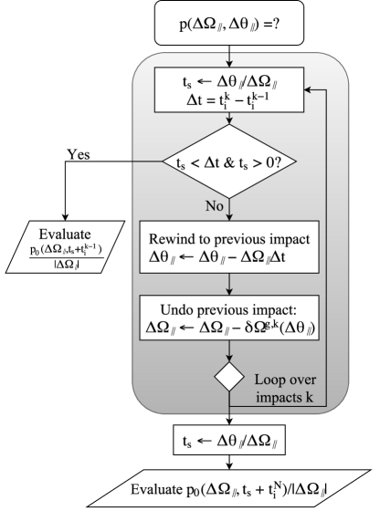
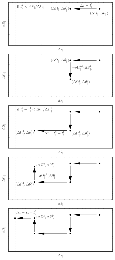
The probability $p(\Delta\Omega_{\parallel},\Delta\theta_{\parallel})$ can then be evaluated by rewinding the phase-space position to all previous impacts, starting with the most recent one, and undoing their effect on $\Delta\Omega_{\parallel}$ to determine $(\Delta\Omega_{\parallel}^{0},\Delta\theta_{\parallel}^{0},t_{i}^{l})$. We do this by rewinding until $\Delta\theta_{\parallel}=0$ between two of the impacts or until the effect of all impacts during the history of the stream has been undone. We then evaluate the release probability as in Equation (2). This algorithm is presented in detail in the flowchart in Figure 3 and illustrated in Figure 4. We could similarly undo the impact of angle kicks $\delta\theta_{\parallel}^{g}$, but we ignore angle kicks because they are small (see discussion above and below).

The probability $p(\Delta\Omega_{\perp},\Delta\theta_{\perp}|\Delta\Omega_{\parallel},\Delta\theta_{\parallel})$ can be evaluated in a similar manner and ideally in parallel with the computation of $p(\Delta\Omega_{\parallel},\Delta\theta_{\parallel})$. That is, we again determine $\Delta\theta_{\parallel}$ at all impacts in between the present time and when the point $(\Delta\mathbf{\Omega},\Delta\boldsymbol{\theta})$ was stripped, starting with the most recent impact, and undo the kicks $\delta\Omega^{g}_{\perp}$ in the perpendicular direction in the same manner as for $\Delta\Omega_{\parallel}$. At the time of stripping determined from the $(\Delta\Omega_{\parallel},\Delta\theta_{\parallel})$ history in the previous paragraph, we then evaluate the release distribution $p_{0}(\Delta\Omega_{\perp}^{0},\Delta\theta_{\perp}^{0}|\Delta\Omega_{\parallel},\Delta\theta_{\parallel})$, which may also depend on time.

Being able to evaluate $p(\Delta\mathbf{\Omega},\Delta\boldsymbol{\theta})$, we can evaluate moments of this probability distribution function by direct numerical integration. This includes the density $p(\Delta\theta_{\parallel})$ as a function of $\Delta\theta_{\parallel}$ and the mean parallel frequency $\langle\Delta\Omega_{\parallel}\rangle(\Delta\theta_{\parallel})$. These are the two main moments that we focus on in the rest of this paper. We compute these as

$$p(\Delta\theta_{\parallel}) =\int\mathrm{d}\Delta\Omega_{\parallel}\,p(\Delta\Omega_{\parallel},\Delta\theta_{\parallel})\,,$$ (3)

$$\langle\Delta\Omega_{\parallel}\rangle(\Delta\theta_{\parallel}) =\frac{1}{p(\Delta\theta_{\parallel})}\,\int\mathrm{d}\Delta\Omega_{\parallel}\,\Delta\Omega_{\parallel}\,p(\Delta\Omega_{\parallel},\Delta\theta_{\parallel})\,,$$ (4)

that is, we use that $\int\mathrm{d}\Delta\Omega_{\perp}\mathrm{d}\Delta\theta_{\perp}p(\Delta\Omega_{\perp},\Delta\theta_{\perp}|\Delta\Omega_{\parallel},\Delta\theta_{\parallel})=1$, because for a given $(\Delta\Omega_{\parallel},\Delta\theta_{\parallel})$ all $(\Delta\Omega_{\perp},\Delta\theta_{\perp})$ get shifted by the same amount. Other moments that are important for the mean track $(\mathbf{x},\mathbf{v})(\Delta\theta_{\parallel})$ of the stream in configuration space are $\langle\Delta\Omega_{\perp}\rangle(\Delta\theta_{\parallel})$ and $\langle\Delta\theta_{\perp}\rangle(\Delta\theta_{\parallel})$. Kicks in the perpendicular direction are always much smaller than those in the parallel direction, because the ratio between the perpendicular and parallel frequency kicks is essentially the ratio of the eigenvalues of $\partial\mathbf{\Omega}/\partial\mathbf{J}$ again and this ratio is small for tidal streams. Unlike kicks in the parallel direction, which always push the stream material away from the point of impact (Erkal & Belokurov, 2015a), kicks in the perpendicular direction can be positive or negative depending on the relative orientation of the stream and the fly-by velocity. Thus, we both expect kicks in the perpendicular direction to be small and to cancel out if many impacts occur.

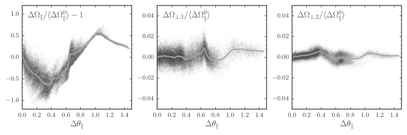
We test this explicitly using mock–data simulations of the GD-1-like stream described in $\mathsection$ 2.1. We generate mock $(\Delta\mathbf{\Omega},\Delta\boldsymbol{\theta})$ data with the method from $\mathsection$ 3.1 for a set of 61 impacts with masses between $10^{5}\,\mathrm{M}_{\odot}$ and $10^{9}\,\mathrm{M}_{\odot}$ sampled using the procedure in $\mathsection$ 2.3. The frequencies as a function of $\Delta\theta_{\parallel}$ are displayed in Figure 5 normalized by the frequency of the smooth stream as a function of $\Delta\theta_{\parallel}$ to focus on the deviations induced by impacts. It is clear that the deviations in the perpendicular direction are indeed much smaller than those in the parallel direction, with the ratio approximately equal to that of the eigenvalues of $\partial\mathbf{\Omega}/\partial\mathbf{J}$. In Appendix A we test this assumption further by comparing mock streams generated by only applying kicks in the parallel direction to full $N$-body simulations of impacts. We find good agreement between these $N$-body simulations and the formalism that only applies parallel frequency kicks (that is, no perpendicular frequency kicks and no angle kicks). In what follows, we will therefore focus on the two-dimensional phase–space distribution $p(\Delta\Omega_{\parallel},\Delta\theta_{\parallel})$ and we only apply the kicks to the parallel frequency, as these dominate the observed structure of tidal streams.

Figure 6: Illustration of the line-of-parallel-angle algorithm to efficiently compute $p(\Delta\Omega_{\parallel},\Delta\theta_{\parallel})$ for a set of $\Delta\Omega_{\parallel}$ at fixed $\Delta\theta_{\parallel}$. The initially vertical line $\Delta\Omega_{\parallel}$ at fixed $\Delta\theta_{\parallel}$ is propagated backwards through two impacts (solid and dashed gray lines). The propagation starts with the most recent impact (top three panels), using a piecewise-linear representation of minus the kick (solid gray line in the top two panels; zero kick is given by the horizontal gray line; we show minus the kick, because the effect of the kick is removed in the backward propagation). This creates a piecewise-linear transformation of the initially vertical $(\Delta\theta_{\parallel},\Delta\Omega_{\parallel})$ line (black line in the middle panel) that can then be propagated through the previous impact in the same manner (bottom three panels). After the line has been propagated through all impacts, we know the release times and initial frequencies that make up the vertical line at the final time. The unperturbed release probability can then be evaluated to give the probability everywhere along the line. As in Figure 4, parts of the line that reach $\Delta\theta_{\parallel}=0$ at an intermediate stage (between impacts before the first one) are not propagated through earlier impacts.

3.3 A line-of-parallel-angle approach to computing $p(\Delta\Omega_{\parallel},\Delta\theta_{\parallel})$

Figure 7: Density $p(\Delta\theta_{\parallel})$ and mean parallel frequency $\langle\Delta\Omega_{\parallel}\rangle(\Delta\theta_{\parallel})$ for a single impact. The left panel displays the density for a single encounter $1.3\,\mathrm{Gyr}$ ago of the GD-1-like mock stream with a $10^{8}\,\mathrm{M}_{\odot}$ dark–matter subhalo with an impact parameter of $525\,\mathrm{pc}$, a fly-by velocity of $160\,\mathrm{km\ s}^{-1}$, and with a closest approach at $\Delta\theta_{\parallel}=0.6$. The solid line in the top, left panel shows the perturbed density, the dashed line gives the density in the absence of an encounter, and the histogram displays the density obtained from mock-stream data sampled as in $\mathsection$ 3.1. The bottom, left panel compares different methods for computing the density: the black curve shows the difference between the density computed using only the linear part of the piecewise-polynomial representation of the $\delta\Omega_{\parallel}^{g}$ kick (Equation [3.3.1]) and including the higher-order parts (Equation [12]); the gray line displays the difference between the higher-order calculation and a direct numerical integration of $p(\Delta\Omega_{\parallel},\Delta\theta_{\parallel})$ using a generic adaptive integrator. The right panels show the same for $\langle\Delta\Omega_{\parallel}\rangle(\Delta\theta_{\parallel})$, with the mock-stream data presented as a grayscale background in the top, right panel. The break around $\Delta\theta_{\parallel}\approx 0.1$ is due to the part of the stream released after the impact (that is therefore unperturbed) and the perturbed part meeting at this angle; this break is unphysically hard here because the impacts occur instantaneously in our calculation. The piecewise-linear approximation of the kick allows one to compute the density and $\langle\Delta\Omega_{\parallel}\rangle(\Delta\theta_{\parallel})$ to much better than $1\,\%$ and is about three orders of magnitude faster than using direct numerical integration.

While it is possible and straightforward to compute moments of $p(\Delta\Omega_{\parallel},\Delta\theta_{\parallel})$ by direct numerical integration, for the $\mathcal{O}(100)$ number of impacts that is expected for old tidal streams within a few tens of kpc from the Galactic center this becomes prohibitively expensive and numerically difficult. As an example, the direct numerical evaluation of $\langle\Delta\Omega_{\parallel}\rangle(\Delta\theta_{\parallel})$ for 30 impacts of $10^{6}\,\mathrm{M}_{\odot}$ dark–matter halos happening all at the same time for 200 values of $\Delta\theta_{\parallel}$ takes approximately a half hour on a single cpu. Full simulations with impacts happening at a range of times and a wide range of masses would therefore take prohibitively long. The approximate method that we describe in this section reduces the computational time for this example to 0.1 s—a speed-up of about a factor of 20,000—and allows us to compute $\langle\Delta\Omega_{\parallel}\rangle(\Delta\theta_{\parallel})$ and the stream density simultaneously for full, realistic simulations in a few minutes on a single cpu.

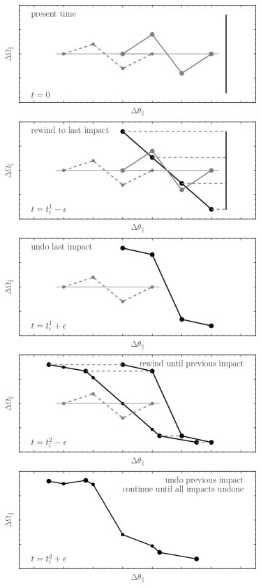
The approximate method that we develop in this section works similarly to the method for the direct evaluation of $p(\Delta\Omega_{\parallel},\Delta\theta_{\parallel})$, but rather than running a single $(\Delta\Omega_{\parallel},\Delta\theta_{\parallel})$ point through all impacts between the present time and the time that this point was released from the progenitor, we run all values of $\Delta\Omega_{\parallel}$ at a given $\Delta\theta_{\parallel}$ through all of the past impacts that they have experienced since their release. We call this approach the “line-of-parallel-angle” approach to computing $p(\Delta\Omega_{\parallel},\Delta\theta_{\parallel})$ as it considers the history of a line of $\Delta\Omega_{\parallel}$ at constant (present-day) $\Delta\theta_{\parallel}$. The essence of this approach is that when we approximate each impact as a piecewise-linear function of $\Delta\theta_{\parallel}$, an initially straight line in $(\Delta\Omega_{\parallel},\Delta\theta_{\parallel})$ remains piecewise linear throughout all past impacts and to fully characterize it we only need to track the breakpoints of this piecewise-linear representation and the linear dependence between each two breakpoints. Eventually we end up with a piecewise-linear representation of the phase–space coordinates $(\Delta\Omega_{\parallel}^{0},\Delta\theta_{\parallel}^{0},t_{i}^{l})$ before the first encountered impact at $t_{i}^{l}$ as a function of the present-day $(\Delta\Omega_{\parallel},\Delta\theta_{\parallel})$. This procedure is illustrated in Figure 6.

We first discuss how this is done in detail for a single impact. In this case, we can also approximately account for higher-order components in a piecewise-polynomial representation of the frequency kicks, allowing us to determine the requisite $\Delta\theta_{\parallel}$ spacing at which to compute the kicks such that the piecewise-linear representation is sufficient. We then describe the algorithm for the general case of multiple impacts occurring at different times.

3.3.1 Single impacts

In the line-of-parallel-angle approach we consider all $\Delta\Omega_{\parallel}$ at a given $\Delta\theta_{\parallel}$ and we want to determine how to evaluate $p(\Delta\Omega_{\parallel},\Delta\theta_{\parallel})$ in terms of the release probability $p_{0}(\Delta\Omega_{\parallel}^{0},t_{s})$. For a single impact giving a kick $\delta\Omega_{\parallel}^{g,1}(\Delta\theta_{\parallel})$ a time $t_{i}^{1}$ in the past we first determine the maximum $\Delta\Omega_{\parallel}$ for which the point $(\Delta\Omega_{\parallel},\Delta\theta_{\parallel})$ was released before the impact: $\Delta\Omega_{\parallel}^{\mathrm{max}}=\Delta\theta_{\parallel}/t_{i}^{1}$. Any $\Delta\Omega_{\parallel}>\Delta\Omega_{\parallel}^{\mathrm{max}}$ must have been released after the impact and for these $\Delta\Omega_{\parallel}$ we have that $p(\Delta\Omega_{\parallel},\Delta\theta_{\parallel})=p_{0}(\Delta\Omega_{\parallel},\Delta\theta_{\parallel})=p_{0}(\Delta\Omega_{\parallel},t_{s})/|\Delta\Omega_{\parallel}|$. For $\Delta\Omega_{\parallel}\leq\Delta\Omega_{\parallel}^{\mathrm{max}}$ we need to determine the release $\Delta\Omega_{\parallel}$ by undoing the kick due to the impact.

We build a piecewise-polynomial representation of $\delta\Omega_{\parallel}^{g,1}(\Delta\theta_{\parallel})$ by computing this function at a set of $\Delta\theta_{\parallel}$ and constructing a spline function of a given order that goes through these data. This representation has the form

$$\begin{split}\delta\Omega_{\parallel}^{g,1}(\Delta\theta_{\parallel})=\sum_{k}c_{bk}\left(\Delta\theta_{\parallel}\right.&\left.-x_{b}\right)^{k}\,,\\ &x_{b}\leq\Delta\theta_{\parallel}<x_{b+1}\,,\end{split}$$ (5)

for a set of breakpoints $\{x_{b}\}$. For this set, we can compute the present $\Delta\Omega_{\parallel}$ as

$$\Delta\Omega_{\parallel,b}=\frac{\Delta\theta_{\parallel}-x_{b}}{t_{i}^{1}}\,.$$ (6)

The sequence of breakpoints is reversed in this way, because $\Delta\Omega_{\parallel,b}$ increases for decreasing $x_{b}$. The set $\{\Delta\Omega_{\parallel,b}\}$ represents the $\Delta\Omega_{\parallel}$ at the present time at which the kicks $\delta\Omega_{\parallel}^{g,1}(\Delta\theta_{\parallel})$ at time $t_{i}^{1}$ have a breakpoint for the line-of-parallel-angle at fixed present $\Delta\theta_{\parallel}$. The coefficients of the piecewise-polynomial representation of the kicks for a value $\Delta\Omega_{\parallel}$ are those of the smallest $\Delta\Omega_{\parallel,b}$ with $\Delta\Omega_{\parallel,b}\geq\Delta\Omega_{\parallel}$. The breakpoints $\{x_{b}\}$ are the gray dots in the top panel of Figure 6 (for the solid gray curve) and the corresponding $\{\Delta\Omega_{\parallel,b}\}$ are the black dots on the black line in the second panel.

We can then compute $p(\Delta\Omega_{\parallel},\Delta\theta_{\parallel})$ for $\Delta\Omega_{\parallel}\leq\Delta\Omega_{\parallel}^{\mathrm{max}}$ as

$$p (\Delta\Omega_{\parallel},\Delta\theta_{\parallel})=p_{0}\left(\Delta\Omega_{\parallel}-\delta\Omega_{\parallel}^{g,1}\left(\Delta\theta_{\parallel}-\Delta\Omega_{\parallel}\,t_{i}^{1}\right),\Delta\theta_{\parallel}-\Delta\Omega_{\parallel}\,t_{i}^{1}\right)\,,$$

$$=p_{0}\left(\Delta\Omega_{\parallel}-\sum_{k}c_{bk}\left(\Delta\theta_{\parallel}-\Delta\Omega_{\parallel}\,t_{i}^{1}-x_{b}\right)^{k},\Delta\theta_{\parallel}-\Delta\Omega_{\parallel}\,t_{i}^{1}\right)\,$$

$$\qquad\qquad\qquad x_{b}\leq\Delta\theta_{\parallel}<x_{b+1}\,,$$

$$=p_{0}\left(\Delta\Omega_{\parallel}-\sum_{k}c_{bk}\,[t_{i}^{1}]^{k}\left(\Delta\Omega_{\parallel,b}-\Delta\Omega_{\parallel}\right)^{k},\Delta\theta_{\parallel}-\Delta\Omega_{\parallel}\,t_{i}^{1}\right)\,$$

$$\qquad\qquad\qquad\Delta\Omega_{\parallel,b}<\Delta\Omega_{\parallel}\leq\Delta\Omega_{\parallel,b+1}\,.$$ (7)

The final right-hand side can be easily evaluated in terms of the release probability as $p_{0}(\tilde{\Delta\Omega_{\parallel}},t_{s})/|\tilde{\Delta\Omega_{\parallel}}|$ with $\tilde{\Delta\Omega_{\parallel}}=\Delta\Omega_{\parallel}-\sum_{k}c_{bk}\,[t_{i}^{1}]^{k}\left(\Delta\Omega_{\parallel,b}-\Delta\Omega_{\parallel}\right)^{k}$ and $t_{s}=(\Delta\theta_{\parallel}-\Delta\Omega_{\parallel}\,t_{i}^{1})/\tilde{\Delta\Omega_{\parallel}}$. Thus, we have a direct piecewise representation of $p(\Delta\Omega_{\parallel},\Delta\theta_{\parallel})$ for all $\Delta\Omega_{\parallel}$ at fixed $\Delta\theta_{\parallel}$.

To compute moments of $p(\Delta\Omega_{\parallel},\Delta\theta_{\parallel})$ we proceed as follows. The density is

$$p(\Delta\theta_{\parallel})=\int\mathrm{d}\Delta\Omega_{\parallel}\,p(\Delta\Omega_{\parallel},\Delta\theta_{\parallel})\,,$$ (8)

which can be written in terms of the piecewise representation of $p(\Delta\Omega_{\parallel},\Delta\theta_{\parallel})$ as

$$\begin{split}p&(\Delta\theta_{\parallel})=\int_{\Delta\Omega_{\parallel}^{\mathrm{max}}}^{\infty}\mathrm{d}\Delta\Omega_{\parallel}\,p_{0}(\Delta\Omega_{\parallel},\Delta\theta_{\parallel})\\ &+\sum_{b}\int_{0}^{\Delta\Omega_{\parallel,b+1}-\Delta\Omega_{\parallel,b}}\mathrm{d}w\,p_{0}(\Delta\Omega_{\parallel,b+1}-w-\sum_{k}c_{bk}\,[t_{i}^{1}]^{k}w^{k},\\ &\quad\qquad\qquad\qquad\qquad\qquad\qquad\Delta\theta_{\parallel}-\Delta\Omega_{\parallel}\,t_{i}^{1})\,.\end{split}$$ (9)

This remains a fully general, exact expression that can be evaluated for any release probability (including, for example, release of bursts of stars at pericentric passages).

For the fiducial model of Bovy (2014), $p_{0}(\Delta\Omega_{\parallel},\Delta\theta_{\parallel})=p_{0}(\Delta\Omega_{\parallel},t_{s})/|\Delta\Omega_{\parallel}|=\mathcal{N}(\Delta\Omega_{\parallel}|\Delta\Omega^{m},\sigma^{2}_{\Omega,1})$ if $t_{s}<t_{d}$; this is a Gaussian distribution with mean $\Delta\Omega^{m}$ and variance $\sigma^{2}_{\Omega,1}$. In this case, we can write the density as

$$p (\Delta\theta_{\parallel})=\int_{\Delta\Omega_{\parallel}^{\mathrm{max}}}^{\infty}\mathrm{d}\Delta\Omega_{\parallel}\,\mathcal{N}(\Delta\Omega_{\parallel}|\Delta\Omega^{m},\sigma^{2}_{\Omega,1})$$

$$\quad+\sum_{b\geq b_{0}}\int_{0}^{\Delta\Omega_{\parallel,b+1}-\Delta\Omega_{\parallel,b}}\!\!\!\!\!\!\!\!\!\!\!\!\!\mathrm{d}w\,\mathcal{N}(\Delta\Omega_{\parallel,b+1}-w-\sum_{k}c_{bk}\,[t_{i}^{1}]^{k}w^{k})$$

$$\approx\int_{\Delta\Omega_{\parallel}^{\mathrm{max}}}^{\infty}\mathrm{d}\Delta\Omega_{\parallel}\,\mathcal{N}(\Delta\Omega_{\parallel}|\Delta\Omega^{m},\sigma^{2}_{\Omega,1})$$

$$\quad+\sum_{b\geq b_{0}}\int_{0}^{\Delta\Omega_{\parallel,b+1}-\Delta\Omega_{\parallel,b}}\mathrm{d}w\,\mathcal{N}(\Delta\Omega_{\parallel,b+1}-c_{b0}-(1+c_{b1}\,t_{i}^{1})w)$$

$$\qquad\left[1+\frac{\Delta\Omega_{\parallel,b+1}-c_{b0}-(1+c_{b1}t_{i}^{1})w-\Delta\Omega^{m}}{\sigma^{2}_{\Omega,1}}\,\sum_{k>1}c_{bk}\,[t_{i}^{1}]^{k}w^{k}\right]\,,$$ (10)

where we have Taylor-expanded the integrand of the second integral around $w=0$ up to first order and the sum is only over frequency-ranges that were released between $t_{d}$ and $t_{i}^{1}$ (denoted as $b\geq b_{0}$; see below). These integrals can be performed analytically. The first term in the square brackets returns the density up to linear order in the piecewise-polynomial kick representation:

$$p (\Delta\theta_{\parallel})\approx\frac{1}{2}\left[1+\mathrm{erf}\left(\frac{1}{\sqrt{2}\sigma_{\Omega,1}}\left[\Delta\Omega^{m}-\Delta\Omega_{\parallel}^{\mathrm{max}}\right]\right)\right]$$

$$+\sum_{b\geq b_{0}}\frac{1}{2(1+c_{b1}t_{i}^{1})}\,\left[\mathrm{erf}\left(\frac{1}{\sqrt{2}\sigma_{\Omega,1}}\left[\Delta\Omega_{\parallel,b+1}-c_{b0}-\Delta\Omega^{m}\right]\right)\right.-$$

$$\left.\mathrm{erf}\left(\frac{1}{\sqrt{2}\sigma_{\Omega,1}}\left[\Delta\Omega_{\parallel,b}-c_{b0}-\Delta\Omega^{m}-c_{b1}\,t_{i}^{1}(\Delta\Omega_{\parallel,b+1}-\Delta\Omega_{\parallel,b})\right]\right)\right]$$ (11)

The second term adds

$$\begin{split}&\sum_{b\geq b_{0}}-\frac{1}{2}\sum_{j=0}^{\mathrm{order}+1}\,E(u,l;j+1)\times\Bigg{[}(-\sqrt{2})^{j+1}\,\sigma_{\Omega,1}^{j-1}\,\\ &\ \ \sum_{k>1}\frac{c_{bk}\,[t_{i}^{1}]^{k}}{(1+c_{b1}\,t_{i}^{1})^{k+1}}\binom{k}{j}\left(\Delta\Omega_{\parallel,b+1}-c_{b0}-\Delta\Omega^{m}\right)^{k-j}\Bigg{]}\,,\end{split}$$ (12)

where $u$ is the argument of the first error function in the sum over $b$ in Equation (3.3.1) and $l$ is the argument of the second error function in the same equation; the sum over $j$ runs up to the order of the piecewise polynomial plus one. The factor $E(u,l;n)$ is defined as

$$E(u,l;n)=\int_{l}^{u}\,\mathrm{d}t\,\frac{2}{\sqrt{\pi}}\,e^{-t^{2}}\,t^{n}\,,$$ (13)

which can be efficiently computed using the recurrence relations

$$E(u,l;0) =\mathrm{erf}(u)-\mathrm{erf}(l)\,,$$ (14)

$$E(u,l;1) =-\frac{1}{\sqrt{\pi}}\left(e^{-u^{2}}-e^{-l^{2}}\right)\,,$$ (15)

$$E(u,l;n) =-\frac{1}{\sqrt{\pi}}\left(e^{-u^{2}}\,u^{n-1}-e^{-l^{2}}\,l^{n-1}\right)$$ (16)

$$\ \ +\frac{n-1}{2}\,E(u,l;n-2)\,.$$

To finish our discussion of how to evaluate $p(\Delta\theta_{\parallel})$ approximately using the line-of-parallel-angle approach, we need to determine the lower limit $b_{0}$ of the integration. This lower limit is obtained by finding the segment where the line-of-parallel-angle switches from being released after $t_{d}$ to being released before $t_{d}$ (which is impossible). In the linear approximation, this interval is that for which the equation

$$\begin{split}\left[\Delta\Omega_{\parallel,b+1}-c_{b0}-(1+c_{b1}\,t_{i}^{1})x\right]&(t_{d}-t_{i}^{1})=\\ &\Delta\theta_{\parallel}-(\Delta\Omega_{\parallel,b+1}-x)\,t_{i}^{1}\,,\end{split}$$ (17)

has a solution within the interval, i.e., $0\leq x<\Delta\Omega_{\parallel,b+1}-\Delta\Omega_{\parallel,b}$. To obtain a better approximation of the interval, we then adjust the lower limit of this interval such that it starts from the value of $x_{0}$ that solves this equation: $\Delta\Omega_{\parallel,b_{0}}\rightarrow\Delta\Omega_{\parallel,b_{0}+1}-x_{0}$.

The calculation of other moments of $p(\Delta\Omega_{\parallel},\Delta\theta_{\parallel})$ is similar and we only discuss the first moment of $\Delta\Omega_{\parallel}$ such that we can compute the mean parallel frequency $\langle\Delta\Omega_{\parallel}\rangle(\Delta\theta_{\parallel})$. We find that the linear terms of the kicks produce

$$\langle\Delta\Omega_{\parallel}\rangle\,p(\Delta\theta_{\parallel})=$$

$$\quad\frac{1}{2}\left[\sigma_{\Omega,1}\sqrt{\frac{2}{\pi}}\,\exp\left(-\frac{1}{2\sigma^{2}_{\Omega,1}}\left[\Delta\Omega^{m}-\Delta\Omega_{\parallel}^{\mathrm{max}}\right]^{2}\right)\right.$$

$$\left.\quad\quad\ \ +\Delta\Omega^{m}\left(1+\mathrm{erf}\left[\frac{1}{\sqrt{2}\sigma_{\Omega,1}}\left(\Delta\Omega^{m}-\Delta\Omega_{\parallel}^{\mathrm{max}}\right)\right]\right)\right]$$

$$+\sum_{b\geq b_{0}}\left(\Delta\Omega_{\parallel,b+1}+\frac{\Delta\Omega^{m}+c_{b0}-\Delta\Omega_{\parallel,b+1}}{1+c_{b1}\,t_{i}^{1}}\right)p_{b}(\Delta\theta_{\parallel})$$

$$\quad+\frac{\sigma_{\Omega,1}}{\sqrt{2\pi}(1+c_{b1}\,t_{i}^{1})^{2}}\times$$

$$\ \ \left[\exp\left(-\frac{1}{2\sigma^{2}_{\Omega,1}}\left[\Delta\Omega_{\parallel,b}-c_{b0}-\Delta\Omega^{m}-c_{b1}\,t_{i}^{1}(\Delta\Omega_{\parallel,b+1}-\Delta\Omega_{\parallel,b})\right]^{2}\right)\right.$$

$$\ \ \left.-\exp\left(-\frac{1}{2\sigma^{2}_{\Omega,1}}\left[\Delta\Omega_{\parallel,b+1}-c_{b0}-\Delta\Omega^{m}\right]^{2}\right)\right]\,,$$ (18)

where $p_{b}(\Delta\theta_{\parallel})$ is the summand in Equation (3.3.1). The higher-order polynomial coefficients in the first-order Taylor expansion of Equation (3.3.1) add

$$\begin{split}\sum_{b\geq b_{0}}&\Delta\Omega_{\parallel,b+1}\,p^{h}_{b}(\Delta\theta_{\parallel})\\ &+\frac{1}{2}\sum_{j=0}^{\mathrm{order}+2}\,E(u,l;j+1)\,\times\Bigg{[}(-\sqrt{2})^{j+1}\,\sigma^{j-1}_{\Omega,1}\\ &\ \sum_{k>1}\frac{c_{bk}\,[t_{i}^{1}]^{k}}{(1+c_{b1}\,t_{i}^{1})^{k+2}}\,\binom{k+1}{j}\,(\Delta\Omega_{\parallel,b+1}-c_{b0}-\Delta\Omega^{m})^{k-j+1}\Bigg{]}\,,\end{split}$$ (19)

where $p^{h}_{b}(\Delta\theta_{\parallel})$ is the summand in Equation (12).

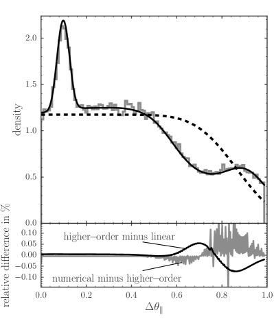
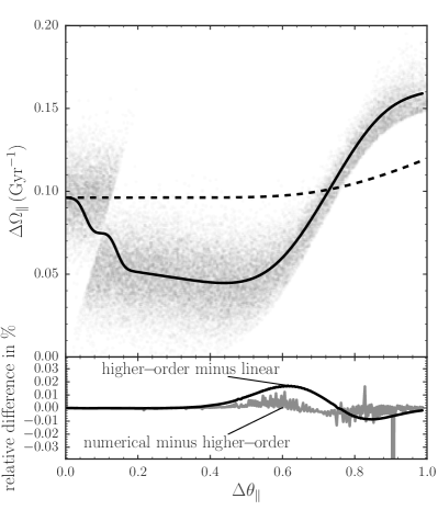
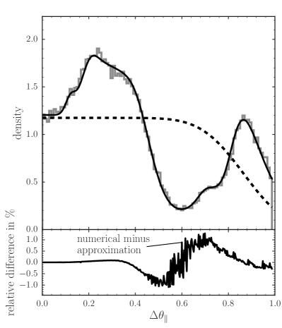
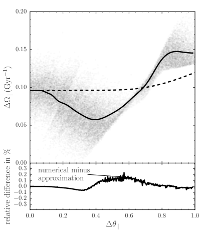
As an example of these calculations, Figure 7 displays the density and mean parallel frequency $\langle\Delta\Omega_{\parallel}\rangle(\Delta\theta_{\parallel})$ of the GD-1-like mock stream after an encounter with a single $10^{8}\,\mathrm{M}_{\odot}$ dark–matter halo. In this figure, we compare the approximations above with (a) the structure obtained using mock data generated as described in $\mathsection$ 3.1 above and (b) direct numerical integrations of $p(\Delta\Omega_{\parallel},\Delta\theta_{\parallel})$—evaluated using the method of $\mathsection$ 3.2. All four different methods agree very well. The bottom panels of Figure 7 compare the computed density and $\langle\Delta\Omega_{\parallel}\rangle(\Delta\theta_{\parallel})$ for the direct numerical integration and using the approximate expressions above. These all agree to less than $0.1\,\%$. The differences between only including the linear part of the piecewise-polynomial representation of the impact kick (Equations [3.3.1] and [3.3.1]) and including the higher-order parts to first order (Equations [12] and [19] are small and only substantial near the impact point. The numerical integration has significant noise at the $0.1\,\%$ level due to the breakpoints in the kick representation and the sharp lower edge in $\Delta\Omega_{\parallel}$ that separates regions of phase–space that can and cannot be populated by the stream. These latter issues are much more significant when considering multiple impacts.

Using the approximation in Equations (3.3.1) allows one to compute $p(\Delta\theta_{\parallel})$ at a single $\Delta\theta_{\parallel}$ in approximately 0.1 ms on a single cpu in a pure Python implementation. Including the higher-order terms in Equations (12) takes about ten times as long, because of the recursion necessary in Equations (14)-(16). Computing the density at a single $\Delta\theta_{\parallel}$ using direct numerical integration of $p(\Delta\Omega_{\parallel},\Delta\theta_{\parallel})$ takes approximately $115$ ms, or more than 1300 times longer than using the piecewise-linear approximation of the kicks. The computation times for $\langle\Delta\Omega_{\parallel}\rangle(\Delta\theta_{\parallel})$ are similar.

When considering multiple impacts below, we will only allow these to occur on a grid of times. We presented the procedure in this section for a single impact, but it can in practice be applied to all impacts that occur at the same time. This can be done by combining all of the individual-kick $\delta\Omega_{\parallel}^{g,j}$ that occur at a given impact time into a single $\delta\Omega_{\parallel}^{g}$ for that time and working with the piecewise-polynomial representation of the combined kick.

3.3.2 Multiple impacts

Figure 8: Same as Figure 7, but for multiple impacts. The GD-1-like mock stream has in this case encountered four dark–matter halos with masses $\approx 10^{7}\,\mathrm{M}_{\odot}$ at times between $1.3\,\mathrm{Gyr}$ and $4.3\,\mathrm{Gyr}$ spaced $1\,\mathrm{Gyr}$ apart, with fly-by velocities of $160\,\mathrm{km\ s}^{-1}$, $152.5\,\mathrm{km\ s}^{-1}$, $229\,\mathrm{km\ s}^{-1}$, and $161\,\mathrm{km\ s}^{-1}$. All four encounters have impact parameters between $0.5$ and $2.5$ scale radii of the dark–matter halos and all have a closest approach with a similar part of the stream, at current $\Delta\theta_{\parallel}$ between 0.6 and 0.75. Thus, the effect of the multiple encounters strongly overlaps. The approximate density $p(\Delta\theta_{\parallel})$ and $\langle\Delta\Omega_{\parallel}\rangle(\Delta\theta_{\parallel})$ agrees with that obtained from mock data. The approximation agrees with the direct numerical evaluation to about $1\,\%$ for the density and better for $\langle\Delta\Omega_{\parallel}\rangle(\Delta\theta_{\parallel})$, while being a factor of 100 faster.

Figure 9: Example perturbed stream densities (left panel) and stream tracks (right panel) computed using the formalism of $\mathsection$ 3.3.2. Each curve in the left panel displays the density compared to that for the unperturbed stream when impacting the GD-1-like mock stream with a set of subhalos with the masses indicated next to the curve and otherwise sampled using the procedure of $\mathsection$ 2.3. The rate of impacts for each mass is that corresponding to its mass decade (e.g., $10^{5}$ to $10^{6}\,\mathrm{M}_{\odot}$ for $10^{5.5}\,\mathrm{M}_{\odot}$): $\approx 43.3$ for $10^{5}$ to $10^{6}\,\mathrm{M}_{\odot}$, $\approx 13.7$ for $10^{6}$ to $10^{7}\,\mathrm{M}_{\odot}$, $\approx 4.3$ for $10^{7}$ to $10^{8}\,\mathrm{M}_{\odot}$, and $\approx 1.4$ for $10^{8}$ to $10^{9}\,\mathrm{M}_{\odot}$. The mean track $\langle\Delta\Omega_{\parallel}\rangle(\Delta\theta_{\parallel})$ in parallel frequency for the same 4 simulations is shown in the right panel. The dashed lines in both panels give the locus where the ratio of perturbed-to-smooth density/track is equal to one. The deviation from one is multiplied by a factor of 3 for the two lowest mass sets of impacts in the right panel. The structure induced by different mass decades has a similar density amplitude for all masses (albeit slightly lower for lower masses), but different masses induce structure on different scales. The same holds for the deviations in the mean track, except that the amplitude decreases faster with decreasing mass.

Figure 10: Same as Figure 9, but showing four examples with impacts sampled from the entire $10^{5}$–$10^{9}\,\mathrm{M}_{\odot}$ mass range using the procedure of $\mathsection$ 2.3. The combination of impacts of different masses induces structure on a wide range of scales, which is especially clear in the density.

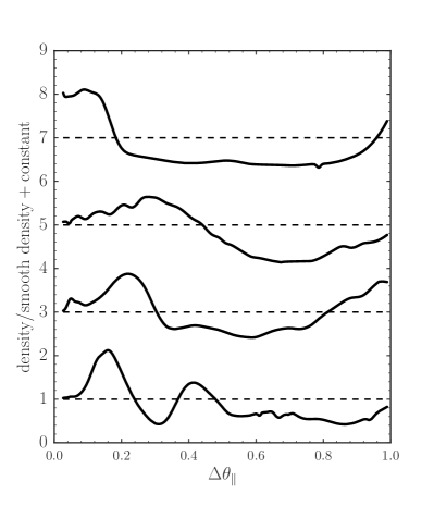
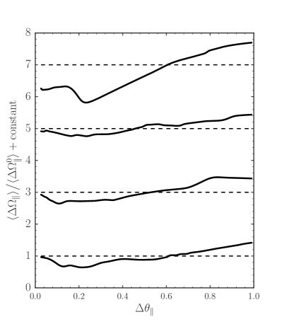
To rapidly compute the stream structure under the influence of multiple impacts, we proceed in a similar manner as for the piecewise-linear approximation for the single-impact case above. We start by combining all individual kicks $\delta\Omega_{\parallel}^{g}$ that occur at the same impact time $t_{i}^{j}$ into a single $\delta\Omega_{\parallel}^{g,j}$ that is applied a time $t_{i}^{j}$ in the past. We then order the kicks in reverse chronological sequence, that is, starting with the most recent one, with indexing starting at one. By propagating a line-of-parallel-angle through all previous impacts in the piecewise-linear approximation of the kicks $\delta\Omega_{\parallel}^{g,j}$, we can form a piecewise-linear representation of this line before all impacts that we can then apply the linear formalism from the previous section to. This procedure is illustrated in Figure 6. This propagation requires one to track each piecewise-linear segment as it goes through all previous impacts and to split up each segment into multiple segments to account for the breakpoints of previous impacts. For this it is necessary to update the coefficients of the piecewise-linear representation of the line-of-parallel-angle to account for the impacts and the splitting up of segments. In the following paragraphs, we describe a simple method to track all of this that emerges from writing out this straightforward, but complicated procedure. We discuss how this algorithm is arrived at in more detail in Appendix B.

We start in the same manner as for a single impact by computing $\Delta\Omega_{\parallel}^{\mathrm{max}}$, the maximum $\Delta\Omega_{\parallel}$ that was released before the final impact: $\Delta\Omega_{\parallel}^{\mathrm{max}}=\Delta\theta_{\parallel}/t_{i}^{1}$. All $\Delta\Omega_{\parallel}>\Delta\Omega_{\parallel}^{\mathrm{max}}$ were stripped from the progenitor after the final impact and we can therefore again evaluate the unperturbed $p_{0}(\Delta\Omega_{\parallel},\Delta\theta_{\parallel})$ to obtain $p(\Delta\Omega_{\parallel},\Delta\theta_{\parallel})$. We then compute the set of breakpoints $\{\Delta\Omega_{\parallel,b}\}$ using Equation (6) corresponding to the final impact $t_{i}^{1}$. With each breakpoint, we associate a set of parallel angles $\{\Delta\theta_{\parallel,b}\}$ and times $\{t_{b}\}$ that are all set to $\Delta\theta_{\parallel}$ and $t_{i}^{1}$, respectively

$$\Delta\theta_{\parallel,b} =\Delta\theta_{\parallel}\,,$$ (20)

$$t_{b} =t_{i}^{1}\,.$$ (21)

In Figure 6, the initial set of $\{\Delta\Omega_{\parallel,b}\}$ are the large black dots on the black line in the second panel.

We further associate with each breakpoint (a) $\{x_{b}\}$, the set of breakpoints for the first kick, (b) $\{d^{b}_{0}\}$ and $\{d_{1}^{b}\}$, the constant and linear coefficients for each piecewise-polynomial segment of the first kick (denoted $c_{b0}$ and $c_{b1}$ in $\mathsection$ 3.3.1), (c) $\{\mathrm{d}\Omega_{b}\}$ defined as

$$\mathrm{d}\Omega_{b}=-d^{b}_{0}-d_{1}^{b}\,(\Delta\theta_{\parallel,b}-x_{b})\,,$$ (22)

the frequency correction from the final kick for each segment, and (d) a set of coefficients $\{c_{b0}\}$, $\{c_{b1}t\}$, and $\{c_{bx}\}$ set to

$$c_{b0} =d_{0}^{b}\,,$$ (23)

$$c_{b1}t =d_{1}^{b}\,t_{i}^{1}\,,$$ (24)

$$c_{bx} =0\,.$$ (25)

By updating these breakpoint-associated arrays through previous impacts, we can trace the line-of-parallel-angle to its initial state.

After undoing the effect of the final impact, we have a piecewise-linear representation of the initial line-of-parallel-angle characterized by its breakpoints $\{\Delta\Omega_{\parallel,b}\}$ and up-to-linear polynomial coefficients $\{d_{0}^{b}\}$ and $\{d_{1}^{b}\}$ (see the middle panel of Figure 6). We also have the parallel angle of each breakpoint at $t_{i}^{1}$: $\Delta\theta_{\parallel}-\Delta\Omega_{\parallel}\,t_{i}^{1}$. A segment $b$ then arrives at the time of the second-to-last impact at the parallel angles

$$\Delta\theta_{\parallel}-(t_{i}^{2}-t_{i}^{1})\,\mathrm{d}\Omega_{b}-\Delta\Omega_{\parallel}\,[t_{i}^{2}-(t_{i}^{2}-t_{i}^{1})\,(1+c_{b1}t)]\,.$$ (26)

We thus update the $\{\Delta\theta_{\parallel,b}\}$ and $\{t_{b}\}$ as

$$\Delta\theta_{\parallel,b} \rightarrow\Delta\theta_{\parallel,b}-(t_{i}^{2}-t_{i}^{1})\,\mathrm{d}\Omega_{b}\,,$$ (27)

$$t_{b} \rightarrow t_{b}+(t_{i}^{2}-t_{i}^{1})\,(1+c_{b1}t)\,,$$ (28)

such that the segment $b$ arrives at the parallel angles

$$\Delta\theta_{\parallel,b}-\Delta\Omega_{\parallel}\,t_{b}\,,$$ (29)

similar to the expression for how each original segment arrives at the final kick. Like in Equation (6), we can then determine the $\Delta\Omega_{\parallel}$ for each current segment and for each breakpoint $x_{b^{\prime}}$ of the second-to-last impact as

$$\Delta\Omega_{\parallel,bb^{\prime}}=\frac{\Delta\theta_{\parallel,b}-x_{b^{\prime}}}{t_{b}}\,,$$ (30)

We only keep those breakpoints ${\Delta\tilde{\Omega}_{\parallel,bb^{\prime}}}$ for each segment $b$ that fall within the $]\Delta\Omega_{\parallel,b},\Delta\Omega_{\parallel,b+1}]$ range of the segment and add it to the current set of breakpoints

$$\{\Delta\Omega_{\parallel,b}\}\rightarrow\{\Delta\Omega_{\parallel,b}\}\cup\{\Delta\tilde{\Omega}_{\parallel,bb^{\prime}}\}\,.$$ (31)

The new breakpoints $\{\Delta\tilde{\Omega}_{\parallel,bb^{\prime}}\}$ are the small black dots in the fourth panel of Figure 6; the total set is both the small and large black dots (from the previous iteration) in this panel.

Having established the set of breakpoints that describes the combined effect of the final two impacts in a piecewise-linear manner, we proceed to undo the effect of the second-to-last impact on $\Delta\Omega_{\parallel}$. For this we need to subtract the piecewise-linear representation of $\delta\Omega_{\parallel}^{g,2}$ between each two breakpoints corresponding to the second-to-last kick. To keep track of this, we first need to update

$$c_{b0} \rightarrow c_{b0}+t_{b}\,d_{1}^{b}\,\Delta\Omega_{\parallel,b}\,,$$ (32)

$$c_{bx} \rightarrow c_{bx}+t_{b}\,d_{1}^{b}\,.$$ (33)

These updates are necessary to account for the new breakpoints inserted in Equation (31): this insertion requires the constant term in the piecewise-linear representation of the line-of-parallel-angle to be updated because of the offset between the old and new breakpoints. All of the arrays associated with the breakpoints are then enlarged by the addition of the new breakpoints (Equation [31]), with the values for the new entries set to those corresponding to the old breakpoint associated with the new one. The latter is that breakpoint before which the new breakpoint is inserted. The exception to this rule are the $\{x_{b}\}$, $\{d_{0}^{b}\}$, and $\{d_{1}^{b}\}$, which are set to the second-to-last impact breakpoints and coefficients; those entries in the sequence for old breakpoints are set to the value of the new breakpoint associated with the old breakpoint. The objective of these is to track the effect of the latest impact. We undo the effect of the second-to-last impact by updating

$$c_{b0} \rightarrow c_{b0}+d_{0}^{b}\,,$$ (34)

$$c_{b1}t \rightarrow c_{b1}t+d_{1}^{b}\,t_{b}\,,$$ (35)

$$\mathrm{d}\Omega_{b} \rightarrow\mathrm{d}\Omega_{b}-d_{0}^{b}+d_{1}^{b}\,(\Delta\theta_{\parallel,b}-x_{b})\,.$$ (36)

In these updates, parts of the line-of-parallel-angle that must have been released at times between $t_{i}^{2}$ and $t_{i}^{1}$ are automatically left unchanged, because for these we have already arrived at their unperturbed values for which we can evaluate $p_{0}(\Delta\Omega_{\parallel},\Delta\theta_{\parallel})$.

Thus, we arrive at the same form of piecewise-linear representation of the line-of-parallel-angle before the second-to-last impact as we had before the last impact. We can then repeat the procedure given here for the second-to-last impact for all previous impacts. The time differences in Equations (27) and (28) becomes those between the previous impact and the current impact, i.e., $(t_{i}^{3}-t_{i}^{2})$ for the third-to-last impact. Otherwise the procedure is the same. After all impacts have been corrected for, $c_{b0}$ receives a final update

$$c_{b0}\rightarrow c_{b0}-c_{bx}\,\Delta\Omega_{\parallel,b}\,.$$ (37)

This update is again part of the correction of the constant term of later impacts when the breakpoints of earlier impacts are inserted into the sequence of breakpoints, thus breaking a linear segment of a later impact into multiple segments (this is described in detail in Appendix B). At the end of this procedure, we have the full representation of the line-of-parallel-angle before the first impact and we can thus evaluate $p(\Delta\Omega_{\parallel},\Delta\theta_{\parallel})$ as $p_{0}(\Delta\Omega_{\parallel},\Delta\theta_{\parallel})$.

With the representation of the line-of-parallel-angle arrived at here, we can evaluate moments of $p(\Delta\Omega_{\parallel},\Delta\theta_{\parallel})$ in the piecewise-linear approximation of the kicks using the expressions in Equation (3.3.1) for the density and Equation (3.3.1) for $\langle\Delta\Omega_{\parallel}\rangle(\Delta\theta_{\parallel})$, respectively, making the substitution $c_{b1}t_{i}^{1}\rightarrow c_{b1}t$. To determine the lower limit $b_{0}$ of the sum, we solve an equation similar to (17), namely,

$$\begin{split}\left[\Delta\Omega_{\parallel,b+1}-c_{b0}-(1+c_{b1}t)x\right]&(t_{d}-t_{i}^{N})=\\ &\Delta\theta_{\parallel,b}-(\Delta\Omega_{\parallel,b+1}-x)\,t_{b}\,,\end{split}$$ (38)

but now using the time $t_{i}^{N}$ of the first impact on the left-hand side. The lower limit $b_{0}$ is determined to be the segment for which the solution $x_{0}$ satisfies $\Delta\Omega_{\parallel,b}<x_{0}\leq\Delta\Omega_{\parallel,b+1}$ and we again adjust the lower limit of this segment to be $\Delta\Omega_{\parallel,b_{0}}\rightarrow\Delta\Omega_{\parallel,b_{0}+1}-x_{0}$.

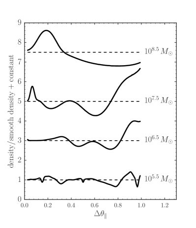
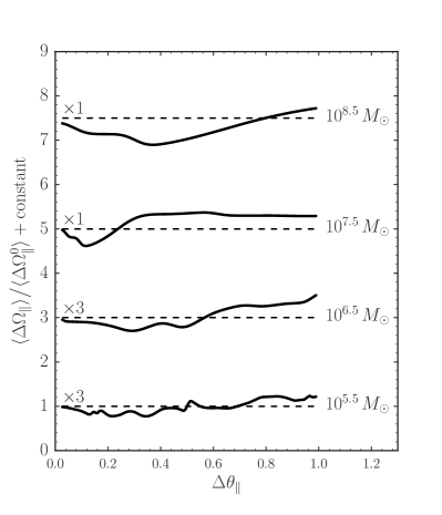
An example of the formalism from this section is displayed in Figure 8. We calculate the effect of four encounters with dark–matter halos with masses $\approx 10^{7}\,\mathrm{M}_{\odot}$ (in detail, $10^{7}\,\mathrm{M}_{\odot}$, $10^{7.25}\,\mathrm{M}_{\odot}$, $10^{6.75}\,\mathrm{M}_{\odot}$, $10^{7.5}\,\mathrm{M}_{\odot}$) at times $1.3\,\mathrm{Gyr}$, $2.3\,\mathrm{Gyr}$, $3.3\,\mathrm{Gyr}$, and $4.3\,\mathrm{Gyr}$ in the past. They have fly-by velocities of $160\,\mathrm{km\ s}^{-1}$, $152.5\,\mathrm{km\ s}^{-1}$, $229\,\mathrm{km\ s}^{-1}$, and $161\,\mathrm{km\ s}^{-1}$, impact parameters that are $0.5$, $2$, $1$, and $2.5$ scale radii of the dark–matter halos, and hit at $\Delta\theta_{\parallel}=0.6$, $0.4$, $0.3$ and $0.3$ at the time of impact. Therefore, they all encounter approximately the same part of the stream that is currently located at $\Delta\theta_{\parallel}\approx 0.68$. As such, this set of impacts is a good test of the formalism here, because the effect of the different encounters significantly overlaps. It is clear from Figure 8 that the approximate calculation from this section agrees well with both the density obtained from sampling mock data using the procedure of $\mathsection$ 3.1 and with a direct numerical integration of the moments of $p(\Delta\Omega_{\parallel},\Delta\theta_{\parallel})$. The densities from the approximate and direct-numerical calculations agree to $\approx 1\,\%$, while the mean parallel frequency $\langle\Delta\Omega_{\parallel}\rangle(\Delta\theta_{\parallel})$ agree to a fraction of that. These precisions are much better than what could realistically be observed for real tidal streams.

Further examples of the formalism from this section are shown in Figures 9 and 10. Figure 9 displays the density and mean parallel frequency $\langle\Delta\Omega_{\parallel}\rangle(\Delta\theta_{\parallel})$ for four simulations. Each simulation consists of impacts of a single value of the mass, but with all other impact parameters sampled as in $\mathsection$ 2.3. The number of impacts for each simulation was sampled from the Poisson rate corresponding to the mass decade of each mass (i.e., the $10^{5.5}\,\mathrm{M}_{\odot}$ simulation uses the rate corresponding to the mass range $10^{5}$ to $10^{6}\,\mathrm{M}_{\odot}$); see the caption of Figure 9 for the actual rates. The single $10^{8.5}\,\mathrm{M}_{\odot}$ impact induces a perturbation covering the entire length of the stream in both the density and $\langle\Delta\Omega_{\parallel}\rangle(\Delta\theta_{\parallel})$. Each individual impact with a lower-mass subhalo affects a shorter part of the stream and the typical scale on which structure is induced is set by the mass of the subhalo. The amplitude of the induced density variations is similar for all mass decades, with only slightly lower amplitudes for the lower-mass decades. The structure induced in $\langle\Delta\Omega_{\parallel}\rangle(\Delta\theta_{\parallel})$ behaves similar, although the amplitude decreases more steeply with decreasing mass. Below we quantify these observations by computing the power spectrum of these density and $\langle\Delta\Omega_{\parallel}\rangle(\Delta\theta_{\parallel})$ fluctuations.

Figure 10 gives four examples with impacts covering the entire mass range that we consider in this paper: $10^{5}$ to $10^{9}\,\mathrm{M}_{\odot}$. The density perturbations are typically of order unity and they display structure on all scales. Our formalism properly accounts for the interference between the effect from different impacts and for the dispersion in the stream, i.e., the filling in or further emptying of gaps due to these effects. Figure 10 shows that structure remains visible on all scales even when all of these effects are taken into account. The mean parallel frequency $\langle\Delta\Omega_{\parallel}\rangle(\Delta\theta_{\parallel})$ again displays a similar behavior, but with smaller amplitude fluctuations overall. Comparing the density and $\langle\Delta\Omega_{\parallel}\rangle(\Delta\theta_{\parallel})$, it is clear that features in the density are correlated with those in $\langle\Delta\Omega_{\parallel}\rangle(\Delta\theta_{\parallel})$. For example, the density dip in the top curve at $\Delta\theta_{\parallel}\approx 0.78$ and the dip in the density in the $10^{5.5}\,\mathrm{M}_{\odot}$ simulation in Figure 9 at $\Delta\theta_{\parallel}\approx 0.5$ have a clear counterpart in $\langle\Delta\Omega_{\parallel}\rangle(\Delta\theta_{\parallel})$. From the four examples shown here, it is also clear that on average $\langle\Delta\Omega_{\parallel}\rangle(\Delta\theta_{\parallel})$ gets slightly tilted counter-clockwise with respect to the unperturbed stream track. This is explained by the fact that we do not consider impacts that occur in the opposite arm or beyond the nominal length of the stream. This only affects the structure of the stream on the largest scales and we ignore this effect in what follows as it only has a marginal effect on the fluctuations in the stream induced by substructure that we are most interested in (see further discussion in Appendix C).

Figure 11: Time to compute $p(\Delta\Omega_{\parallel},\Delta\theta_{\parallel})$ for all $\Delta\Omega_{\parallel}$ at a given $\Delta\theta_{\parallel}$ using the line-of-parallel-angle approximation of $\mathsection$ 3.3.2 as a function of the number of impacts at different times. The computational time scales approximately as $N^{2.25}$ for $N$ impacts. The CDM prediction for the number of impacts for the GD-1-like mock stream is approximately 63 impacts (see $\mathsection$ 2.3), for which the line-of-parallel-angle approximation can be computed in $0.3$ s for a single $\Delta\theta_{\parallel}$ and a fine sampling in $\Delta\theta_{\parallel}$ of the structure of the perturbed stream can be computed in about one minute.

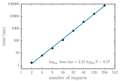
In Figure 8, the approximate calculation is about 100 times faster than the direct numerical integration, with the approximate calculation taking $9$ ms for a single $\Delta\theta_{\parallel}$ on a single cpu. The approximate calculation for multiple impacts in this case is about 100 times slower than that for a single impact (see $\mathsection$ 3.3.1). This is because the procedure to propagate the line-of-parallel-angle through multiple impacts requires one to track all of the associated arrays as described in this section and this is expensive compared to the ease with which expressions (3.3.1) and (3.3.1) can be evaluated. The computational time for each impact is therefore dominated by the operations described in this section, which increase with each previous impact due to the ever larger number of breakpoints to track. Figure 11 shows the computational time for computing the density $p(\Delta\theta_{\parallel})$ at a single $\Delta\theta_{\parallel}$ as a function of the number of impacts at different times (because multiple impacts at the same time do not increase the computational cost). The computational time increases approximately as $N^{2.25}$ for $N$ impacts, essentially because the number of breakpoints to track increases linearly with the number of impacts at different times. As the propagation of the line-of-parallel-angle dominates the computational cost and this propagation returns the entire $p(\Delta\Omega_{\parallel},\Delta\theta_{\parallel})$, all moments can be evaluated simultaneously at approximately zero cost compared to the propagation. Thus, in the case of Figure 8, both the density and mean parallel frequency can be evaluated in a total time of $9$ ms per $\Delta\theta_{\parallel}$, leading to a further factor of two speed-up compared to the numerical evaluation of these moments.

While we do not consider $p(\Delta\Omega_{\perp},\Delta\theta_{\perp}|\Delta\Omega_{\parallel},\Delta\theta_{\parallel})$ here, because its contribution to the present-day stream structure is small (as demonstrated in Figure 5), it is clear that if desired, this probability can be computed in a similar manner as $p(\Delta\Omega_{\parallel},\Delta\theta_{\parallel})$ in the line-of-parallel-angle approach. This is because the kicks $\delta\mathbf{\Omega}^{g}$ only depend on $\Delta\theta_{\parallel}$, such that all $(\Delta\Omega_{\perp},\Delta\theta_{\perp})$ at a given $(\Delta\Omega_{\parallel},\Delta\theta_{\parallel})$ have the same history of $\delta\Omega_{\perp}^{g}$ and induced $\delta\Delta\theta_{\perp}$. This history could be straightforwardly computed by keeping track of the changes in $\Delta\Omega_{\perp}$ and induced changes in $\Delta\theta_{\perp}$ of each segment for all impacts during the backward-propagation of the line-of-parallel-angle above, as long as the piecewise-polynomial representation of each impact’s $\delta\Omega_{\perp}^{g}$ has the same breakpoints as that of its corresponding $\delta\Omega_{\parallel}^{g}$.

3.4 Conversion to configuration space

Figure 12: Power spectra of the fluctuations in the density and the mean track $\langle\Delta\Omega_{\parallel}\rangle(\Delta\theta_{\parallel})$ relative to those in the unperturbed stream for impacts of different masses. Each curve has impacts of a single value for the mass with the rate set by the surrounding mass decade (e.g., that of $10^{7}-10^{8}\,\mathrm{M}_{\odot}$ for $10^{7.5}\,\mathrm{M}_{\odot}$). The left and central panels display the square root of the power spectra of the density and $\langle\Delta\Omega_{\parallel}\rangle(\Delta\theta_{\parallel})$ fluctuations, while the right panel shows the square root of the magnitude of the cross power spectrum between the density and $\langle\Delta\Omega_{\parallel}\rangle(\Delta\theta_{\parallel})$. The $x$-axis is the inverse of the wavenumber, such that small scales are on the left. All curves are the median of at least $1,000$ different simulations. The solid lines are computed using the fiducial simulation setup; with other linestyles we also show the result from increasing the time sampling, the factor $X$ that sets the maximum impact parameter, and the length along the stream at which impacts are considered (see text for details).
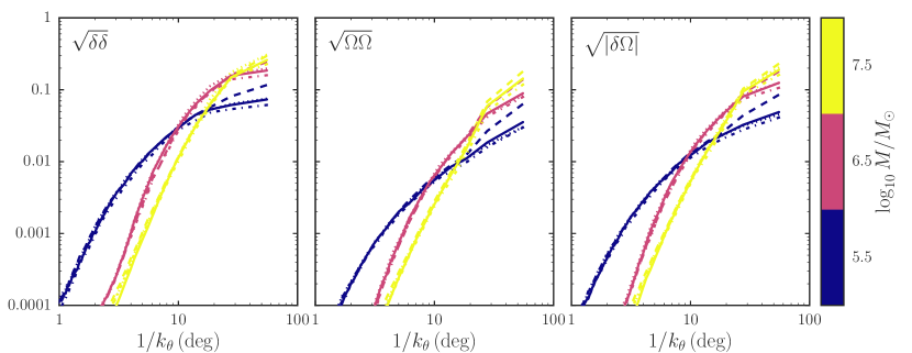
While all the different mass ranges contribute most of their power on the largest scales, the power on smaller scales is cut off in a mass-dependent manner. The power on a particular scale is dominated by the contribution of a single mass range. In particular, the power on a few degree scales is dominated by the effect of $\approx 10^{5}-10^{6}\,\mathrm{M}_{\odot}$ subhalos. Both the density and mean track display fluctuations of a similar magnitude and a similar dependence on scale, although the density fluctuations are typically a factor of a few larger. Fluctuations in the density and the track are strongly correlated.

So far we have discussed how to compute the phase–space structure of a perturbed stream in frequency–angle space. To compare these models to observed data, the models need to be projected into configuration space $(\mathbf{x},\mathbf{v})$. Before discussing how this projection can be performed efficiently, it is important to note the following. The relation between $\Delta\theta_{\parallel}$ and more-easily observable coordinates for the location along a stream (e.g., RA, Galactic longitude $l$, or a custom celestial coordinate frame along the stream) is smooth without any high-frequency power (see, for example, the middle panel of Figure 1). Because the density, say as a function of $l$, is given by $p(l)=p(\Delta\theta_{\parallel})\left|\mathrm{d}\Delta\theta_{\parallel}/\mathrm{d}l\right|$ and $\left|\mathrm{d}\Delta\theta_{\parallel}/\mathrm{d}l\right|$ does not vary rapidly along a stream, the statistical properties as a function of scale (e.g., the power spectrum or bispectrum as discussed below) of $p(l)$ will be very similar to those of $p(\Delta\theta_{\parallel})$. Similarly, we will compute the perturbed stream track by converting the stream track in frequency–angle space to configuration space. Because the perturbations due to subhalo impacts are small, perturbations in observable coordinates are related to those in frequency–angle space through Jacobians that vary smoothly over the length of the stream as in the case of the density. Therefore, the perturbations in observable space will be very similar to those in frequency–angle space except for their overall amplitude.

To convert the density $p(\Delta\theta_{\parallel})$ and the mean track $\langle\Delta\Omega_{\parallel}\rangle(\Delta\theta_{\parallel})$ to configuration space—say, Galactic coordinates $(l,b,D,V_{\mathrm{los}},\mu_{l},\mu_{b})$—we compute the current track of the stream in the absence of perturbations and convert it to configuration space using the iterative method from Bovy (2014) (see $\mathsection$ 2.1). As discussed by Bovy (2014), this procedure returns the track in configuration space at a series of points $\Delta\theta_{\parallel,i}$ along the stream and the Jacobian of the transformation $(\mathbf{\Omega},\boldsymbol{\theta})\rightarrow(\mathbf{x},\mathbf{v})$ at these points. Using these Jacobians, we can then linearize the transformation between $(\mathbf{\Omega},\boldsymbol{\theta})$ and $(\mathbf{x},\mathbf{v})$ (or $(l,b,D,V_{\mathrm{los}},\mu_{l},\mu_{b})$). Improving on Bovy (2014), we linearly interpolate these Jacobians for points $\Delta\theta_{\parallel}$ between the points $\Delta\theta_{\parallel,i}$ (Bovy (2014) used the Jacobian for the nearest $\Delta\theta_{\parallel,i}$ to a given $\Delta\theta_{\parallel}$).

The density $p(l)$ as a function of $l$ then follows from $p(l)=p(\Delta\theta_{\parallel})\left|\mathrm{d}\Delta\theta_{\parallel}/\mathrm{d}l\right|$. The Jacobian can be computed from the Jacobians of $(\Delta\Omega_{\parallel},\Delta\theta_{\parallel})\rightarrow(\mathbf{x},\mathbf{v})$ (in practice, this is most easily done numerically). Below, we will consider the ratio of the perturbed density to that of the unperturbed stream $p(\Delta\theta_{\parallel})/p_{0}(\Delta\theta_{\parallel})$. Because both are converted to $p(l)$ using the same Jacobian, $p(l)/p_{0}(l)=p(\Delta\theta_{\parallel})/p_{0}(\Delta\theta_{\parallel})$.

To convert the track $\langle\Delta\Omega_{\parallel}\rangle(\Delta\theta_{\parallel})$ to configuration space, we simply convert the phase–space points $(\Delta\Omega_{\parallel}=\langle\Delta\Omega_{\parallel}\rangle(\Delta\theta_{\parallel}),\Delta\Omega_{\perp}=0,\Delta\theta_{\parallel},\Delta\theta_{\perp}=0)$ to configuration space (see above for a discussion of why setting $\Delta\Omega_{\perp}=0$ and $\Delta\theta_{\perp}=0$ is a good assumption). Because the perturbations $\langle\Delta\Omega_{\parallel}\rangle(\Delta\theta_{\parallel})-\langle\Delta\Omega_{\parallel}^{0}\rangle(\Delta\theta_{\parallel})$ are small, the linear approximation of the coordinate transformation is precise.

We do not display any examples of perturbations in configuration space like in Figures 9 and 10, because for the reasons discussed at the start of this subsection, the perturbations in configuration space look essentially the same as those in frequency–angle space. In particular, the shape of, e.g., $\langle b\rangle(l)$ is the same as that of $\langle\Delta\Omega_{\parallel}\rangle(\Delta\theta_{\parallel})$. Because the perturbations are to a good approximation only in $\langle\Delta\Omega_{\parallel}\rangle(\Delta\theta_{\parallel})$ (see Figure 5 and associated discussion), all projections of the perturbed stream track in configuration space are tracing the same perturbations and they are therefore almost completely correlated. This implies that measurements of a stream’s location in different coordinates can be stacked to obtain better measurements of the perturbed stream.

$\mathsection$ 4 Tidal stream power spectra

The line-of-parallel-angle approach for computing the density and mean track allows the efficient computation of the structure of a tidal stream perturbed by the $\mathcal{O}(100)$ expected number of impacts with dark–matter subhalos that properly takes into account the dispersion within the stream and the overlapping effects of multiple impacts. In this section, we use this to run large suites of simulations for the GD-1-like stream from $\mathsection$ 2.1 and investigate its statistical properties using the one-dimensional power spectrum of density or track fluctuations induced by the perturbations.

Figure 13: Like Figure 12, but for impacts with masses sampled from the full $10^{5}\,\mathrm{M}_{\odot}$ to $10^{9}\,\mathrm{M}_{\odot}$ range. The curves with colors following the colorbar use dark–matter subhalos with a Hernquist profile following different $r_{s}(M)$ relations that roughly bracket the relation seen for halos in the Via Lactea II simulation; these have $r_{s}$ a factor of 2.5 larger or smaller than the fiducial relation. The lighter blue curve models the dark–matter subhalos as Plummer spheres, with $r_{s}(M)=1.62\,\mathrm{kpc}\,\left(M/10^{8}\,\mathrm{M}_{\odot}\right)^{0.5}$, which produces subhalos with similar concentrations as the fiducial Hernquist model. The gray band shows the interquartile range within which individual simulations lie for the fiducial setup. The concentration of the subhalo modifies the power spectrum on the smallest scales, with larger fluctuations for more compact subhalos. The power spectra are almost indistinguishable at scales larger than a few degrees when the subhalos are modeled with Hernquist or Plummer profiles.

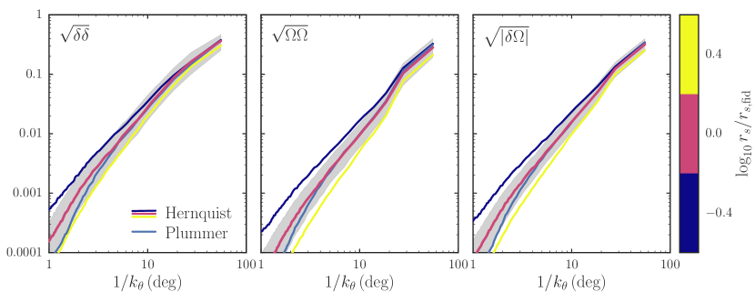
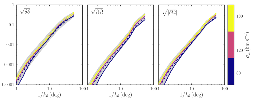
We compute the power spectrum of the density fluctuations for a single simulation by taking the perturbed density and dividing it by the density of the unperturbed stream (e.g., Figure 10) and computing the one-dimensional power spectrum using a Hann window (e.g., Press et al., 2007). In practice, we use the csd routine in scipy (Jones et al., 2001) and do not divide by the sampling frequency. In all of the figures, we plot the square root of the power spectrum versus the inverse of the frequency, such that the $y$ and $x$ axes represent the typical value of fluctuations at a given spatial scale. In all figures, we perform at least 1,000 simulations of the specified setup and display the median power spectra of all of these simulations. We do this, because individual power spectra scatter are noisy and scatter around the median. In many figures we also show the interquartile range of the $>1,000$ simulations as a gray band, such that the scatter among different realizations can be assessed.

Similarly, we compute the power spectrum of fluctuations in the mean track $\langle\Delta\Omega_{\parallel}\rangle(\Delta\theta_{\parallel})$ by dividing the perturbed location of the track by the unperturbed location and follow the same procedure as for the density. To investigate the amount of correlation between fluctuations in the density and in the track, we also compute the cross power spectrum and look at the square root of its absolute value (i.e., we do not consider the phase information here, although that will also contain useful information about the impacts).

In this section, we consider the density and track in frequency–angle space. As discussed above, the stream track is simplest in this space, because all of the relevant structure is in the direction parallel to the stream, which is simplest in this coordinate system. In a later section we will compute power spectra of the density and track as they would be observed, but these are very similar to the power spectra in frequency–angle space for the reasons discussed above in $\mathsection$ 3.4.

Our sampling setup has a number of parameters that need to be fixed. We investigate these in detail in Appendix C and briefly describe the results from these tests here. We only allow impacts to happen at a set of equally-spaced discrete times along the past orbit of the stream, because of the computational savings that come from having multiple impacts at the same time (multiple impacts at the same time do not increase the computational cost of the line-of-parallel-angle algorithm). The sampling of the discrete set of times needs to be high enough such that the structure of the stream is not affected by the discrete time sampling. In Appendix C we find that the statistical properties of the perturbed GD-1-like tidal stream converge quickly when the time sampling is increased above a few times and we use a standard value of 64 times, which corresponds to a time interval of $\approx 140\,\mathrm{Myr}$. This is somewhat smaller than the radial period of the stream, which is $400\,\mathrm{Myr}$, which makes intuitive sense. In general, we therefore conclude that allowing impacts to happen at times sampled slightly more frequently than the radial period of the orbit is sufficient for investigating the statistical properties of perturbed streams (as long as the time interval is not a simple fraction of the period).

We further have to choose a value for the parameter $X$, which describes the maximum impact parameter that we consider in the equation $b_{\mathrm{max}}=X\,r_{s}(M)$. Appendix C demonstrates that the largest-scale structure of the stream converges very slowly with increasing $X$, but the small-scale structure converges for $X>1$. We fix $X=5$ as the standard value in our simulations and it should be kept in mind that the largest-scale modes at $1/k_{\theta}\gtrsim 25^{\circ}$ in the power spectrum (and bispectrum below) are not fully converged and likely underestimated by a few tens of percent. The largest-scale structure of a stream is significantly affected by distant encounters.

Figure 14: Like Figure 13, but varying the age of the stream. The solid lines vary the age of the stream from the fiducial value of $9\,\mathrm{Gyr}$ to $4.5\,\mathrm{Gyr}$ and $13.5\,\mathrm{Gyr}$, while keeping the product of the age and the stream’s velocity-dispersion parameter $\sigma_{v}$ constant. This keeps the current length of the stream the same. Because the impact rate depends linearly on the age at fixed length (cf. Equation [1]), the younger/older stream has a rate of impacts that is 50 % lower / 50 % higher. The blue and yellow dashed curves vary the age while keeping the number of impacts the same. The dashed lines with the same color as the fiducial age are rescalings of the fiducial power spectrum with factors of $0.5$ and $1.5$. Changing the age of the stream while keeping the rate of impacts the same changes the power spectrum of the track fluctuations (middle panel) by approximately these two factors. However, adjusting the age and using the appropriate number of impacts for the adjusted age gives much larger changes. The density power spectra or the density–track cross power spectra do not change linearly when the number of impacts increases due to the older age of the stream.

Figure 15: Like Figure 13, but varying the rate of impacts (top row) and using a subhalo mass spectrum that is exponentially cut-off below a given mass. In the top row, the rate of impacts is increased or decreased by factors of 3 and 10; the rate of impacts with masses between $10^{5}\,\mathrm{M}_{\odot}$ and $10^{9}\,\mathrm{M}_{\odot}$ therefore varies between 6.27 and 627. The dashed curves display the fiducial power spectrum rescaled by the square root of the changes in rate; this is the expected dependence if all impacts produce independent fluctuations in the stream. The power spectrum of mean track fluctuations is remarkably close to this expectation. This makes the mean-track power spectrum a powerful and unambiguous probe of the dark–matter subhalo mass spectrum (however, it is also the most difficult to measure; see below). The density hews close to the expectation from independent fluctuations when the rate is lowered, but the power spectrum is severely depressed when the rate is increased. For the case of a ten times higher rate, this is because the stream essentially gets destroyed by the subhalos, leaving a density peak near the progenitor without a stream. The bottom row demonstrates that a low-mass cut-off in the subhalo mass spectrum leads to a cut-off in the stream power spectra, at the expected locations from the single-mass simulations in Figure 12. In the bottom row, the fiducial case, which has no cut-off, is colored according to a cut-off at $10^{4.5}\,\mathrm{M}_{\odot}$, which is below the minimum mass that we consider.

Figure 16: Like Figure 13, but varying the velocity dispersion $\sigma_{h}$ of the population of dark–matter subhalos. The solid lines vary $\sigma_{h}$ by $50\,\%$ from the fiducial value of $120\,\mathrm{km\ s}^{-1}$ to $180\,\mathrm{km\ s}^{-1}$ (yellow curve) and to $80\,\mathrm{km\ s}^{-1}$ (purple curve). Because the impact rate depends linearly on $\sigma_{h}$ (cf. Equation [1]), the hotter/colder dark–matter population has rate of impacts that is 50 % higher / 33 % lower. The dashed curves are rescalings of the fiducial power spectrum with factors of $\sqrt{3/2}$ and $\sqrt{2/3}$, appropriate if the impacts would act independently. The track power spectrum lies close to this expectation, while the density power spectrum and the density–track cross power spectrum vary less with $\sigma_{h}$.

Finally, we investigate how far along the stream we have to consider impacts. Stellar streams do not have sharp edges and subhalo perturbations could push low-surface brightness stream material towards the higher-density part of the stream. In our fiducial setup we simply consider impacts up to the length of the stream as defined at the end of $\mathsection$ 2.1 evaluated at the time of the impact. The convergence tests in Appendix C demonstrate that impacts further along the stream have a negligible impact on the present-day structure of the stream (up to its nominal length). However, if one were only computing the perturbed structure of a stellar stream up to, say, half the length of the stream (because, e.g., high-quality observations only extend over that range), it would still be necessary to consider impacts over the full length of the stream, as their effect at later times could impact the observed half of the stream.

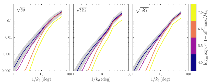
To understand the level at which power is induced on different scales by different decades in subhalo mass, we perform simulations of impacts with impact rates for a single mass decade while setting the mass of all subhalos to the (logarithmically) central value in the range. That is, we perform simulations of $M=10^{7.5}\,\mathrm{M}_{\odot}$ subhalo impacts with a rate of 4.3 that is the expected number for the range $10^{7}\,\mathrm{M}_{\odot}$ to $10^{8}\,\mathrm{M}_{\odot}$ and compute the power spectra and cross power spectra of the density and track fluctuations. We do the same for $10^{6.5}\,\mathrm{M}_{\odot}$ and $10^{5.5}\,\mathrm{M}_{\odot}$ impacts. Figure 9 displays some examples of the perturbed stream densities and tracks produced by these kinds of simulations.

The power spectra for the different mass decades are displayed in Figure 12. The solid lines represent the results from the fiducial simulation setup, with impacts considered at $64$ different times, impact parameters up to $5\times r_{s}(M)$, and out to the length of the stream (as defined at the end of $\mathsection$ 2.1). The other line styles summarize the results from the convergence tests in Appendix C discussed above: The dot-dashed lines consider impacts at 256 different times; these are in almost all cases underneath the solid lines, demonstrating that the power spectra have converged at 64 times. The dotted lines have impacts up to $125\,\%$ times the length of the stream; these are also close to the solid lines. Finally, the dashed curves take into account impacts out to $10\times r_{s}(M)$. These dashed curves deviate from the solid curves on the largest scales, demonstrating that the large-scale structure of the stream is significantly affected by distant encounters ($10\times r_{s}(M)\approx 6\,\mathrm{kpc}$ for $M=10^{7.5}\,\mathrm{M}_{\odot}$). We do not show the result from $>10^{8}\,\mathrm{M}_{\odot}$ impacts, because those are subdominant on all scales for this stream.

It is clear from Figure 12 that the different mass ranges dominate the structure on particular scales for CDM-like impact rates. The highest-mass impacts dominate the structure on the largest scales and lower-mass impacts dominate on smaller scales. Thus, by carefully measuring the power spectrum, the contribution of different mass decades to the impact rate could be determined. Because this rate is a direct reflection of the subhalo mass spectrum, this allows the subhalo mass spectrum to be measured from tidal stream power spectra.

Because of the dispersion in the stream and the dynamics of the induced gaps, the effect of different impacts at the present time overlaps and we need to consider impacts of all masses simultaneously. The power spectra resulting from simulations over the entire mass range of $10^{5}\,\mathrm{M}_{\odot}$ to $10^{9}\,\mathrm{M}_{\odot}$ are displayed in Figure 13. The reddish line represents our fiducial sampling setup. The power spectra considering impacts from all masses closely follow the upper envelope of those from the individual mass decades in Figure 12. This indicates that to a good approximation the total power is simply the combination of the power from each individual mass decade. Therefore, the identification of power on a certain scale with a certain mass decade is robust.

Figure 13 further considers the impact of the radial profile of the dark–matter subhalos. The fiducial model uses a simple $r_{s}(M)$ relation that is close to the average relation in the Via Lactea II simulation (see discussion above). Figure 13 also shows the power spectra when increasing or decreasing $r_{s}(M)$ by a factor of $2.5$, which approximately brackets the mass–concentration relation of Via Lactea II subhalos. Increasing the concentration of the dark–matter subhalos increases the power on small scales, but only has a minor effect on the structure on the largest scales. Figure 13 also shows power spectra for the case where the dark–matter subhalos are modeled as Plummer spheres rather than Hernquist spheres that similarly follow the average mass–concentration relation in Via Lactea II. This leads to very similar power spectra as in the fiducial Hernquist case. Therefore, the concentration is the primary dark–matter-profile parameter that matters.

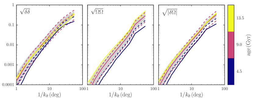
The time since the disruption of the progenitor started—the “age” of the stream—is a quantity that is observationally difficult to establish, as it will generally be different from the age of the stars in the stream. A reasonable upper limit on the age of the stream is the age of the youngest stars near the ends of the stream, because no star formation occurs in low-mass streams. The age of the stream is an important ingredient in any modeling of perturbations to the stream structure due to subhalo impacts, as the encounter rate depends linearly on the age of the stream if the length of the stream is known. This follows from Equation (1), because $t_{d}\,\Delta\Omega^{m}$ is proportional to the length of the stream, leaving a single factor of $t_{d}$ that gives the linear age dependence. At a fixed rate of impacts, the age of the stream affects the time that individual perturbations have to grow and decay (due to internal dispersion and the effect of other impacts).

Figure 14 displays what happens to the various tidal-stream power spectra that we consider when the age of the stream is changed. We vary the age of the stream by $50\,\%$ up or down and adjust the stream’s velocity-dispersion parameter $\sigma_{v}$ by the inverse of this factor, such that the stream remains approximately the same length. The solid lines use the rate that follows directly from Equation (1) and which is thus $50\,\%$ larger or smaller than the fiducial case; we refer to these as the “fully-varied realizations”. This produces large changes in the power spectra. The dashed lines vary the age while keeping the number of encounters the same (thus nominally falling below or above the CDM rate); we denote these as the “constant-rate age realizations”. This produces power spectra that are less different from the standard case. To give a sense of the magnitude of the changes, we display rescaled versions of the fiducial power spectra by factors of $1.5$ and of $0.5$. The fully-varied age realizations lie close to the $1.5$ and $0.5$ lines in the track power spectrum and the cross power spectrum, except on the largest scales for the older realizations. The younger stream’s track power spectrum also falls below the $0.5$ scaling. The constant-rate realizations typically lie closer to the fiducial setup than the $0.5/1.5$ scalings.

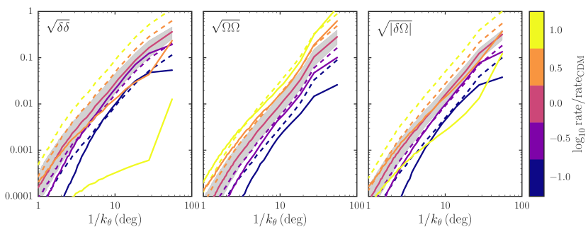
The fully-varied older stream has a significantly suppressed density power spectrum. This is because the large rate of impacts severely batters the stream, making it appear smoother again. We will investigate this effect further below, where we vary the rate of impacts at constant age. The fully-varied younger stream has a track power spectrum that is more reduced from the fiducial case than its density power spectrum is. This is because a subhalo impact immediately gives a large change in $\langle\Delta\Omega_{\parallel}\rangle(\Delta\theta_{\parallel})$ that gets smoothed out at later times. The density perturbation due to a subhalo impact requires time to grow (e.g., Sanders et al. 2016) and only starts to get smoothed by the stream’s dispersion and the effect of other impacts at much later times. It is clear from comparing Figure 14 to the other figures in this section that the age of the stream is an important parameter for the tidal stream power spectra and in particular is more important than the internal structure of the subhalos (Figure 13) or their velocity dispersion (Figure 16 below).

Figure 17: Bispectra of the density and mean-track $\langle\Delta\Omega_{\parallel}\rangle(\Delta\theta_{\parallel})$ fluctuations for simulations with a single value for the mass (those described in Figure 12). The first and second panel from the left display the magnitude of the real and imaginary parts of the bispectrum for the density; the third and fourth panels display the same for the mean track. We only show a one-dimensional slice through the two-dimensional bispectrum at a scale of $\approx 11^{\circ}$. The density has large real and imaginary parts of the bispectrum, because of the asymmetry between troughs and peaks and the higher impact rate at the ends of the stream, respectively. The bispectrum of mean-track fluctuations is smaller, but the imaginary part is large because of the asymmetry of the parallel-frequency kick (i.e., the fact that they always push stream material away from the impact point). The bispectrum is dominated by the highest mass impacts on all scales.

Figure 18: Bispectra like in Figure 17, but for simulations covering the entire mass range $10^{5}\,\mathrm{M}_{\odot}$ to $10^{9}\,\mathrm{M}_{\odot}$. We display the bispectra for the simulations that vary the rate of impacts (those in the top row of Figure 15). The gray band again shows the interquartile range within which individual simulations lie for the fiducial setup. The bispectrum is highly sensitive to the rate of impacts, except that for high rates, the density bispectrum is suppressed because the stream gets destroyed (cf. Figure 15).

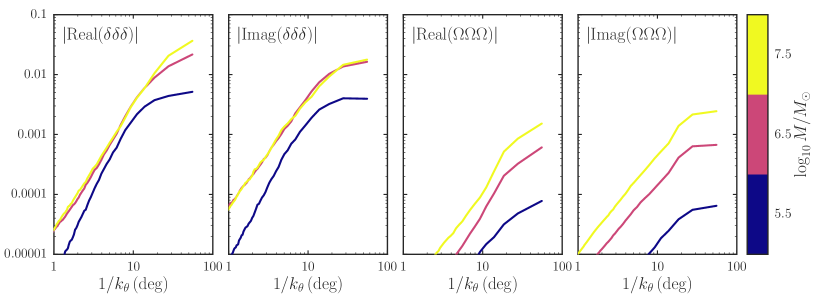
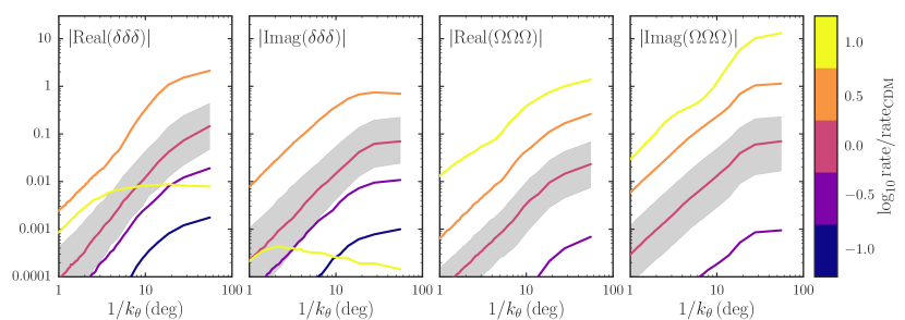
The effect of different impact rates is explored in Figure 15. The top row multiplies the CDM-like rate of impacts over the entire $10^{5}\,\mathrm{M}_{\odot}$ to $10^{9}\,\mathrm{M}_{\odot}$ range by factors of 10, 3, 1/3, and 1/10. The dashed lines display the fiducial, CDM-like power spectra rescaled by the square root of these factors. This is the expected scaling if the impacts give rise to independent fluctuations. The lower-rate density power spectra hew close to this expectation, except on the smallest and largest scales. However, the higher-rate density power spectra are significantly suppressed compared to the fiducial case. The reason for this behavior is that the large number of impacts essentially destroys the stream. Because each impact pushes stream material away from the impact point, the total effect of a large number of impacts is to push a large amount of the stream all the way to the progenitor and the rest far away from the progenitor. As we do not track impacts that happen in the opposite arm of the stream, our modeling does not handle this case very well, but it is clear that the outcome does not produce a realistic stream. Thus, a low density power spectrum due to a low number of dark–matter subhalos would not be confused with a low power spectrum due to a high number of subhalos, because in the latter case the overall morphology of the stream would be very different from that in the former case.

While the density power spectrum reacts non-linearly to a higher or lower rate of subhalo impacts, the track power spectrum changes close to linear over almost the entire factor of 100 difference in the impact rate. The one exception is the case where the rate is lowered by a factor of ten, which is more strongly suppressed than the linear expectation. Because the rate of impacts in this case is only 6.27, this is in large part due to the great Poisson variation in the number of impacts in different realizations. That the case with a ten times higher rate has an approximately $\sqrt{10}$ times greater power than the fiducial CDM-like case, even though the stream is essentially destroyed is a remarkable illustration of the fact that the track power spectrum is a well-behaved tracer of the rate of impacts. The density–track cross power spectrum behaves similarly to the density power spectrum in all cases, although it suffers from less suppression for the higher rates than the density power spectrum.

Comparing Figure 14 to the top panel of Figure 15, we see that varying the age of the stream is approximately equivalent to changing the overall rate of impacts in how it affects the various power spectra. Thus, knowing a stream’s age is important when determining the rate of impacts from the observed power spectrum.

The bottom row of Figure 15 displays what happens when the subhalo mass spectrum has an exponential cut-off below a certain mass. As expected from the behavior of different mass subhalos in Figure 12, the cut-off in the mass spectrum leads to a cut-off in the stream power spectra below the scale at which the cut-off mass starts dominating the power in the stream (e.g., $\approx 10^{\circ}$ for $10^{5.5}\,\mathrm{M}_{\odot}$). This happens similarly in the density and track power spectra and in the cross power spectrum. For a cut-off at $10^{7.5}\,\mathrm{M}_{\odot}$, the power on the largest scales is already suppressed. Therefore, a drop in the power in the density or track of a tidal stream below a certain scale is indicative of a cut-off in the subhalo mass spectrum.

Figure 16 explores what happens to the tidal stream power spectra when we vary the velocity dispersion $\sigma_{h}$ of the dark–matter subhalos. While this parameter can be estimated based on the kinematics of halo stars (e.g., Sirko et al., 2004) or by equilibrium modeling of the dark–matter halo (e.g., Piffl et al., 2015), the velocity distribution of subhalos is not necessarily the same as either of those and is therefore somewhat uncertain (e.g., Diemand et al., 2004). Varying $\sigma_{h}$ changes the overall rate of encounters, which is proportional to $\sigma_{h}$ (see Equation [1]), as well as the velocity distribution of fly-bys. Relative fly-by speeds will typically be larger if $\sigma_{h}$ is larger, which should lead to smaller kicks. Figure 16 demonstrates that the track power spectra again behave simply in that the power scales close to $\sigma_{h}$ (dashed lines). This indicates that any differences in the velocity distribution of fly-bys are subdominant compared to the overall change in the rate. The density power spectra and density–track cross power spectra display smaller changes, with the density being largely insensitive to $\sigma_{h}$ on scales larger than a few degrees.

Similar kinds of simulations that vary the spectral index of the subhalo mass spectrum or the subhalo concentration–mass relation (beyond what was explored in Figure 13), or that change the phase or Galactocentric radius at which the stream is observed, or other variations are straightforward and fast to perform using the line-of-parallel-angle approach from $\mathsection$ 3.3. The exploration in this section focused on some of the most important variations and we postpone further exploration to future work.

$\mathsection$ 5 Tidal stream bispectra

So far we have only considered the power spectrum of the density and track variations induced by dark–matter subhalo impacts. But the density and track changes induced by individual impacts are manifestly non-Gaussian and it should be expected that the fluctuations in the density and track induced by the combination of many impacts might have non-trivial higher-order moments.

In particular, the density variation induced by a single impact some time after the impact is a deep, wide trough with narrow ridges whose height depends on the potential (e.g., Carlberg, 2012; Erkal & Belokurov, 2015a). This profile has a strong up/down asymmetry missed by the power spectrum. The track variation $\langle\Delta\Omega_{\parallel}\rangle(\Delta\theta_{\parallel})$ from a single impact is downward up to a minimum deviation followed by a sharp upturn through the impact point to a maximum upward change that declines further from the impact point (for the leading arm and opposite for the trailing arm; Sanders et al. 2016). This has a strong upstream/downstream asymmetry that is also missed by the power spectrum. Both of these signals should show up strongly in the bispectrum, because the bispectrum’s real part is sensitive to up/down asymmetries and the imaginary part is responsive to left/right asymmetries in one-dimensional signals (Masuda & Kuo, 1981; Elgar, 1987). That the oldest, end part of the stream will have suffered more impacts than the youngest part close to the progenitor will also cause a strong left/right asymmetry (which may provide a method for determining whether a stream is leading or trailing for progenitor-less streams).

Figure 19: Power spectrum for the fiducial simulation setup for the GD-1-like stream (cf. Figure 13), but measuring the density in $\Delta l=0.3^{\circ}$ bins as a function of Galactic longitude rather than $\Delta\theta_{\parallel}$. The gray band shows the interquartile range within which individual simulations lie. The gray horizontal line shows the noise level for $10\,\%$ measurements of the density in each bin, a realistic goal for future experiments.

Figure 20: Like Figure 19, but for the simulations with a single value for the mass (those described in Figure 12). This demonstrates that $10\,\%$ density measurements can determine the number of $>10^{5}\,\mathrm{M}_{\odot}$ dark–matter subhalos.

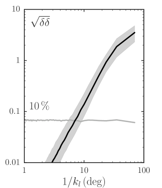
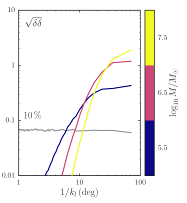
The bispectrum $B(k_{1},k_{2})$ of a signal $f(x)$ is defined as

$$B(k_{1},k_{2})=F^{*}(k_{1}+k_{2})\,F(k_{1})\,F(k_{2})\,,$$ (39)

where $F(k)$ is the Fourier transform of $f(x)$ and $F^{*}(k)$ is its complex conjugate. We compute this using a Rao-Gabr window function with size 7 (Rao & Gabr, 1984). The bispectrum is a two-dimensional function, although it has many symmetries (Rao & Gabr, 1984). We will only display one-dimensional slices through the bispectrum at an intermediate scale $k_{1}$; other slices that are not shown display similar behavior.

Figure 21: Like Figure 19, but for fluctuations of the mean track in observed Galactic latitude, distance, and line-of-sight velocity, as a function of $l$. The horizontal gray lines display the noise level for measurements of the mean location of the track with the given uncertainties. These uncertainties are realistic if $10\,\%$ density measurements are possible. Because all track measurements determine the same underlying one-dimensional $\langle\Delta\Omega_{\parallel}\rangle(\Delta\theta_{\parallel})$ fluctuations, different coordinates are highly correlated and could be combined to provide higher-precision measurements.

Figure 22: Like Figure 21, but for the simulations with a single value for the mass (those described in Figure 12). Because track-location fluctuations are smaller than density fluctuations, track fluctuations are limited to determining the number of $>10^{6}\,\mathrm{M}_{\odot}$ dark–matter subhalos.

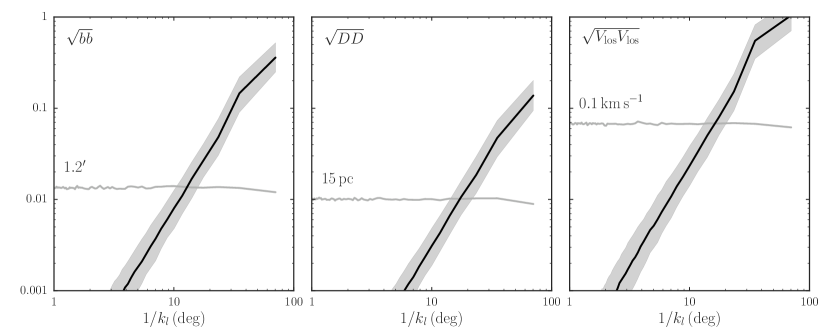
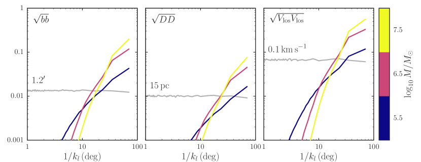
The density and mean-track bispectra for the same single-valued-mass simulations as in Figure 12 are displayed in Figure 17. These represent a one-dimensional slice at $1/k_{1}=11^{\circ}$, a scale at which different mass ranges contribute similarly to the power spectrum (see Figure 12). The bispectra act largely as expected, with a large real part of the density bispectrum because of the trough/ridge asymmetry and a large imaginary part of the track bispectrum because of the upstream/downstream asymmetry. However, the imaginary and real part of the density and track bispectrum, respectively, are only a factor of a few smaller. For the density, the $10^{6}\,\mathrm{M}_{\odot}$ to $10^{7}\,\mathrm{M}_{\odot}$ range and the $10^{7}\,\mathrm{M}_{\odot}$ to $10^{8}\,\mathrm{M}_{\odot}$ range give a similar contribution to the bispectrum, while for the track the $10^{7}\,\mathrm{M}_{\odot}$ to $10^{8}\,\mathrm{M}_{\odot}$ range provides the largest contribution on all scales. This is also the case for other values of $k_{1}$ and we conclude that most of the signal in the bispectrum comes from the highest-mass impacts.

In Figure 18 we show the bispectrum for simulations of the entire mass range $10^{5}\,\mathrm{M}_{\odot}$ to $10^{9}\,\mathrm{M}_{\odot}$ for the fiducial CDM-like setup (red line) and for higher and lower impact rates (same as in the top row of Figure 15). The bispectrum acts in a similar way as the power spectrum when the rate of impacts is varied. Reductions in the rate for the density and any change for the mean track produce well-behaved changes in the bispectrum, but upward changes in the rate suppress the density bispectrum similar to the power spectrum. This is again caused by the destruction of the stream (see discussion of the power spectrum above). Overall, the bispectrum is strongly sensitive to changes in the rate and is therefore an excellent probe of the higher-mass end of the subhalo mass spectrum.

Figure 23: Like Figure 19, but for the cross power spectra of density and track fluctuations. We employ the same noise in both as in Figures 19 and 21 to determine the noise level in the cross correlation. Different cross power spectra are again strongly correlated and could be combined to form more precise measurements.

Figure 24: Same as Figure 20, but for the cross power spectra. At low noise levels, the cross correlation between the density and track fluctuations due to $>10^{5}\,\mathrm{M}_{\odot}$ dark–matter subhalos should be detectable. This would provide an important confirmation of measurements based on the density fluctuations alone.

Figure 25: Bispectra of the density and mean track location in observable coordinates. As in Figures 20 and 22, the density and track are computed in $\Delta l=0.3^{\circ}$ bins in Galactic longitude $l$. The gray horizontal line displays the $2\sigma$ (5 %) upper noise level for Gaussian uncertainties of $10\,\%$ in the density and $1.2^{\prime}$ in the track location $b$ (the median noise is very close to zero for Gaussian uncertainties). The darker, dashed gray curve in the left two panels gives the $2\sigma$ upper noise level when the noise has a Poisson distribution; for $10\,\%$ uncertainties this is close to Gaussian. The bispectrum should be easily measurable in the near future.

Figure 26: Like Figure 25, but for simulations where the rate of impacts is varied (those in the top row of Figure 15). The gray band again shows the interquartile range within which individual simulations lie for the fiducial setup. From this and the previous figure, it is clear that the bispectrum is extremely sensitive to the number of $\gtrsim 10^{6}\,\mathrm{M}_{\odot}$ subhalos.

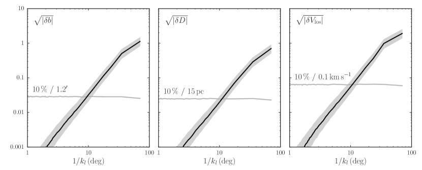
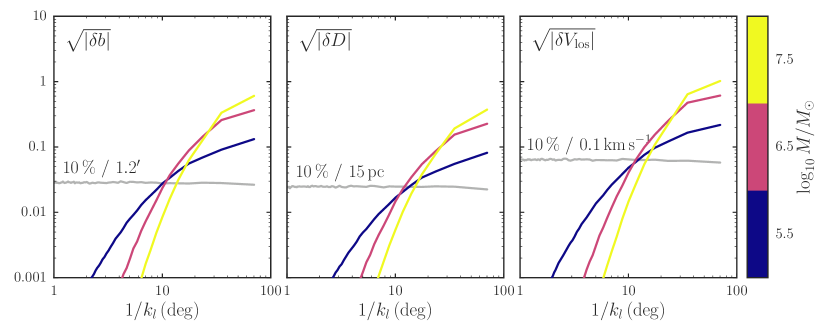
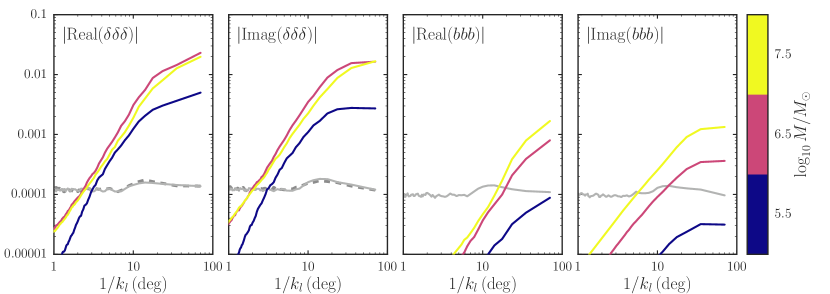
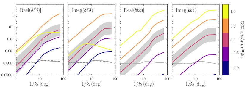
We have also computed the bispectrum for simulations in which the age of the stream is varied (cf. Figure 14). Similar to the power sectrum, changes in the bispectrum due to varying the age are almost equivalent to changes because of rate variations, with approximately the same relation between age and rate as for the power spectrum. Thus, the bispectrum cannot be used to break the degeneracy between age and rate that is inherent in the power spectrum. It is possible that higher-order moments, such as the trispectrum, or the phase contain information on the age of the stream, but we do not investigate this here. The age can also be determined from the observed length and width of a stream—independent of the perturbations due to subhalos—through dynamical modeling of the formation of the stream (e.g., Bovy, 2014; Erkal et al., 2016). Thus, the degeneracy between rate and age will not be a major limitation with future data on streams.

It is straightforward to compute the bispectra of the other simulations for which we discussed the power spectrum in $\mathsection$ 4. We do not show these here, but the bispectra generally behave similarly as the power spectra, i.e., when the power spectrum is increased, so is the bispectrum and vice versa. If the noise in observational determinations of the density and the mean track is well understood, the bispectrum will be a crucial ingredient in any analysis of the structure of tidal streams in terms of subhalo perturbations.

$\mathsection$ 6 Tidal stream power spectra and bispectra in configuration space

As discussed in $\mathsection$ 3.4, we can easily convert the density $p(\Delta\theta_{\parallel})$ and the mean track $\langle\Delta\Omega_{\parallel}\rangle(\Delta\theta_{\parallel})$ to configuration space using a linearized $(\mathbf{\Omega},\boldsymbol{\theta})\rightarrow(\mathbf{x},\mathbf{v})$ transformation. Therefore, we can determine the tidal stream power spectra and bispectra from the preceding sections in configuration space where they are more easily compared to observations. In particular, we convert the density and track to the Galactic coordinate system $(l,b,D,V_{\mathrm{los}},\mu_{l},\mu_{b})$ and use $l$ as the coordinate along the stream (see Figure 1). As argued in $\mathsection$ 3.4, the smoothness of the $(\mathbf{\Omega},\boldsymbol{\theta})\rightarrow(\mathbf{x},\mathbf{v})$ transformation and the small size of the track perturbations implies that the density and track perturbations induced by subhalo impacts are very similar in frequency–angle and configuration space. The scale dependence of the power spectra and bispectra in particular closely tracks that of the power spectra and bispectra in frequency–angle space. Therefore, we only show and discuss the power spectra and bispectra of some of the simulations from $\mathsection$$\mathsection$ 4 and 5. The main advantage of computing the stream properties in configuration space is that it is easier to assess the impact of observational noise and we discuss the contributions from noise in detail.

Figure 27: Model for the Pal 5 stream generated using the method of Bovy (2014) using galpy’s MWPotential2014 for a stream age of $5\,\,\mathrm{Gyr}$, a velocity-dispersion parameter $\sigma_{v}=0.5\,\mathrm{km\ s}^{-1}$, and using the phase-space coordinates of the Pal 5 globular cluster from Fritz & Kallivayalil (2015)’s Table 2 (with a distance to the cluster of $23.2\,\mathrm{kpc}$). The blue line displays the mean stream track in angular coordinates (left panel) and in line-of-sight velocity (right panel), the grayscale shows a sampling of mock stream data from the model, and the red points are the stream positions from Fritz & Kallivayalil (2015) on the left and the velocity measurements from Kuzma et al. (2015) on the right. The angular width of the stream is 15’ FWHM, in good agreement with the measurement of 18’ of Carlberg et al. (2012). The stream model in the MWPotential2014 potential provides an excellent match to the positional and velocity data of the Pal 5 stream.

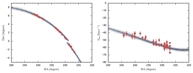
Figure 19 displays the power spectrum of density fluctuations as a function of Galactic longitude for the fiducial CDM-like setup for the GD-1-like stream. Thus, this power spectrum is similar to that in Figure 13, except that it is computed from the density fluctuation that is a function of $l$ rather than $\Delta\theta_{\parallel}$. It is clear that the power spectrum is very similar. That the angular scales are almost the same whether the density is a function of $\Delta\theta_{\parallel}$ or $l$ is due to the fact that the stream is observed between peri- and apocenter; the length of the stream in $\Delta\theta_{\parallel}$ and configuration space is in general different depending on which phase of the stream orbit that the stream is observed at. We have also included the noise contribution when the density of the stream is measured to $10\,\%$ in $0.3^{\circ}$ bins over the entire length of the stream. The noise power spectrum is computed in the same way as the tidal stream power spectrum (both for the density and the track below), by generating 1,000 realizations of Gaussian noise and computing their median. As expected, this noise power spectrum is approximately flat. This noise level is feasible if a clean stream map below the main-sequence turn-off can be constructed with future surveys, e.g., through proper-motion selection.

To determine what dark–matter subhalo masses we are sensitive to, we also compute the density power spectrum for the single-valued-mass simulations of Figure 12. This is shown in Figure 20. These power spectra are again very similar to those in Figure 12 and we see that we can still associate angular scales with specific dark–matter subhalo mass ranges. With $10\,\%$ density measurements we can easily see the fluctuations induced by subhalo with masses down to $10^{5}\,\mathrm{M}_{\odot}$ and potentially even below this mass if the trend in this figure continues. Even with density measurements that are a factor of a few worse, we should still be able to see impacts down to $\approx 10^{5.5}\,\mathrm{M}_{\odot}$.

Going beyond the density, we further compute the mean location of the stream in angular position on the sky $\langle b\rangle(l)$, distance $\langle D\rangle(l)$, and line-of-sight velocity $\langle V_{\mathrm{los}}\rangle(l)$ (the proper motion perturbations are tiny and likely unobservable far into the future). The power spectrum of these three projections of the track for the fiducial setup is shown in Figure 21 (we subtract the unperturbed track rather than dividing by it for these projections). We also include optimistic estimates of the noise in the measured track position in $\Delta l=0.3^{\circ}$ bins. If $10\,\%$ density measurements are possible, then these track measurements are possible as well given the width of the stream (in $b$ and $V_{\mathrm{los}}$) and photometric precision (for the distance). Thus, we should be able to measure the $b$-track power spectrum down to $10^{\circ}$ for this stream and to slightly larger scales for $D$ and $V_{\mathrm{los}}$.

The breakdown of these track power spectra in terms of subhalo mass decades is displayed in Figure 22. These demonstrate that we may be able to measure the contribution to the track power spectra of subhalo masses down to $10^{6}\,\mathrm{M}_{\odot}$. Because each projection of the track ultimately derives from the one-dimensional $\langle\Delta\Omega_{\parallel}\rangle(\Delta\theta_{\parallel})$, the different projections are fully correlated and could in principle be combined to produce a higher signal-to-noise rate measurement of the track power spectrum. This could push the sensitivity down to $10^{5.5}\,\mathrm{M}_{\odot}$ dark–matter subhalos.

Like in frequency–angle space, the density and track fluctuations are strongly correlated, which we can use as another powerful measure of the subhalo mass spectrum. The density-track cross power spectra for the three track projections considered in the previous paragraphs are displayed in Figure 23. The breakdown into different subhalo mass decades is shown in Figure 24. For the same observational uncertainties as for the density and track measurements above, the cross power spectra are observable at scales $\gtrsim 8^{\circ}$, which reaches a sensitivity of $\approx 10^{5.5}\,\mathrm{M}_{\odot}$. The cross power spectra corresponding to the different track projections are again strongly correlated and could be combined to produce higher signal-to-noise-ratio observations. These may increase the sensitivity down to $\approx 10^{5}\,\mathrm{M}_{\odot}$. The cross power spectra combine the sensitivity of the density fluctuations to subhalo impacts with the observational robustness of track fluctuations. They will play a major role in confirming and sharpening the subhalos signal detected in the density fluctuations.

Using the density and mean track in configuration space we can further compute bispectra of the density and mean-track fluctuations. These are shown in Figures 25 and 26 for the same simulations for which we displayed the bispectra in frequency–angle space in Figures 17 and 18. We only show the bispectra of the mean angular location $\langle b\rangle(l)$; those of the mean distance and line-of-sight velocity are similar. It is clear that the bispectra in configuration space are almost the same as those in frequency–angle space. For Gaussian uncertainties, the median noise bispectrum is zero, however, because we display the absolute value, the median noise is simply very small. In Figures 25 and 26, we show the noise as the $5\,\%$ upper limit to the noise level as a gray line for the same assumed noise level in the density and track as for the observed power spectra above. That is, only $5\,\%$ of simulations of the noise are above the gray line. For the density bispectrum, the dashed gray curve displays the same noise level for noise with a Poisson distribution, assuming the $10\,\%$ uncertainties in the relative density come from a Poisson distribution with a mean of $100$ counts. The noise level in the bispectrum is nearly identical for Poisson or Gaussian noise. The bispectrum extends a few orders of magnitude above the noise, which is scale independent. The bispectrum is observable, even if the rate is ten times less than the CDM rate, in which case the power spectrum becomes more difficult to observe for our assumed uncertainties.

$\mathsection$ 7 Density power spectrum of Pal 5

Some measurements of the density of tidal streams already exist (e.g., Odenkirchen et al., 2003; Carlberg et al., 2012; Carlberg & Grillmair, 2013). In this Section, we illustrate the formalism of this paper by performing a measurement of the density power spectrum of the Pal 5 stream and the first rigorous constraint on the number of dark–matter subhalos with masses between $10^{6.5}\,\mathrm{M}_{\odot}$ and $10^{9}\,\mathrm{M}_{\odot}$ using the density data from Ibata et al. (2016).

We build a model for the Pal 5 stream in a smooth potential using the formalism of Bovy (2014). As discussed in $\mathsection$ 2.1, such a model is specified by 8 free parameters in a given gravitational potential: the current phase–space position of the progenitor, the velocity-dispersion parameter $\sigma_{v}$, and the time $t_{d}$ since disruption started. Because the progenitor of the Pal 5 stream is the Pal 5 globular cluster, we can use the measured phase–space position of this cluster as the current phase–space position. We employ the position and velocity from Fritz & Kallivayalil (2015), who measured the proper motion in addition to existing measurements of the celestial position, distance, and line-of-sight velocity of Pal 5. The distance to Pal 5 has some uncertainty and could plausibly lie between $19$ and $24\,\mathrm{kpc}$; we use a distance of $23.2\,\mathrm{kpc}$ as this gives a good match to the stream location. As our model for the Milky Way’s smooth gravitational potential we use MWPotential2014 from Bovy (2015). This potential has been fit to a variety of kinematic data on the bulge, disk, and halo of the Milky Way, as discussed by Bovy (2015). The parameters $\sigma_{v}$ and $t_{d}$ need to be determined from the width and length of the Pal 5 stream. We do not perform a rigorous fit, but simply try a few common-sense values. We find that $\sigma_{v}=0.5\,\mathrm{km\ s}^{-1}$ gives a stream width of $15^{\prime}$ (FWHM), in good agreement with the measurement of Carlberg et al. (2012), who find $18^{\prime}$. We use an age of $t_{d}=5\,\mathrm{Gyr}$ of the stream, which gives a decent match to the data below, although it is not well constrained as the length of the Pal 5 stream has not been measured because the stream hits the edge of the SDSS survey.

We compare our model to the measurements of the location of the Pal 5 stream from Fritz & Kallivayalil (2015) and to line-of-sight velocities for stream members from Kuzma et al. (2015) in Figure 27. The model for the Pal 5 stream using the observed phase–space position of the Pal 5 globular cluster in the MWPotential2014 potential provides an excellent match to the data. This gives additional credence to the MWPotential2014 from Bovy (2015), because many otherwise reasonable models for the Milky Way’s potential fail to give a good match to both the celestial position of the stream and its line-of-sight velocity (see Fritz & Kallivayalil 2015). We employ this Pal 5 model here as a model for the unperturbed stream and apply the formalism from this paper to predict the stream density in the presence of subhalo encounters using the power spectrum.

Figure 28: Star counts for the trailing arm of the Pal 5 stream from Ibata et al. (2016). The top panel displays the background-subtracted counts of stars with $20<g_{0}<23$ and $0.2^{\circ}<\xi<14.3^{\circ}$, along with the polynomial fit that we employ to normalize the star counts in the bottom panel. The bottom panel shows the relative density variations along the stream after dividing out the third-order polynomial fit (orange curve in the top panel).

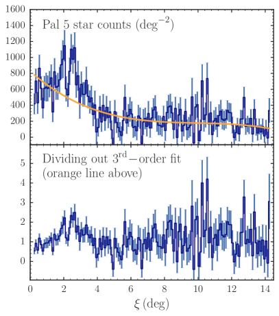
We use the data from Ibata et al. (2016) to determine the density power spectrum along the trailing arm of Pal 5. Ibata et al. (2016) use deep CFHT $g$ and $r$-band data to determine star counts in the vicinity of the Pal 5 stream down to $g_{0}=24$, the deepest map of any known stream. In particular, we use the star counts for the Pal 5 stream in the range $20<g_{0}<23$ from their Figure 7 using their $(\xi,\eta)$ coordinate system. These data are obtained with a simple color–magnitude filter centered on the main-sequence of the Pal 5 globular cluster and it has not been background-subtracted. We use the CFHT photometric data to estimate a constant background level of $\approx 400$ stars deg^-2 and subtract this from the density data. This determination of the Pal 5 density along the trailing arm is shown in the top panel of Figure 28. The background may not be entirely uniform and current data lack a wide enough area away from the stream to determine the importance of the background. Because background variations should be largely uncorrelated with the stream star counts (except, e.g., if variable extinction is important), background variations will simply add power to the power spectrum and lead us to overestimate the number of subhalos from the current data.

The density data in Figure 28 have a clear large-scale trend, with a peak at $\xi<4^{\circ}$. Such a peak is absent in our model, which has a constant stripping rate over time. It is likely that this peak at least partially occurs because of an increase in the stripping rate over the last few orbits, because Pal 5 is close to being fully disrupted (Dehnen et al., 2004). To account for this, we fit a third-order polynomial to the density data and divide this out. The thus normalized density is displayed in the bottom panel of Figure 28. It is this density that we compare to simulations of the effect of subhalos for different rates of impacts and different mass ranges of subhalos. The median uncertainty on the normalized density is $\approx 60\,\%$. The normalization has a big effect on the power on the largest scale, reducing it to $\approx 0.6$ from $\approx 2$. For this reason, we cannot fully use the power on the largest scale to constrain the impact rate below. Power on smaller scales is less affected by this procedure.

Figure 29: Example simulations of the relative density along the trailing arm of the Pal 5 stream. The top panel displays the observed relative density (bottom panel of Figure 28). The three lower panels show example simulations where the model Pal 5 stream from Figure 27 has been perturbed by different rates of impacts between $10^{6}\,\mathrm{M}_{\odot}$ and $10^{9}\,\mathrm{M}_{\odot}$. Rates much smaller than the CDM rate do not typically cause density fluctuations above the noise level, while rates much larger than the CDM rate produce obvious large-scale fluctuations. The CDM example was hand-picked out of a set of $\approx 200$ simulations to be similar to the observed relative density, but it is not atypical; it provides a remarkable match to the observed density.

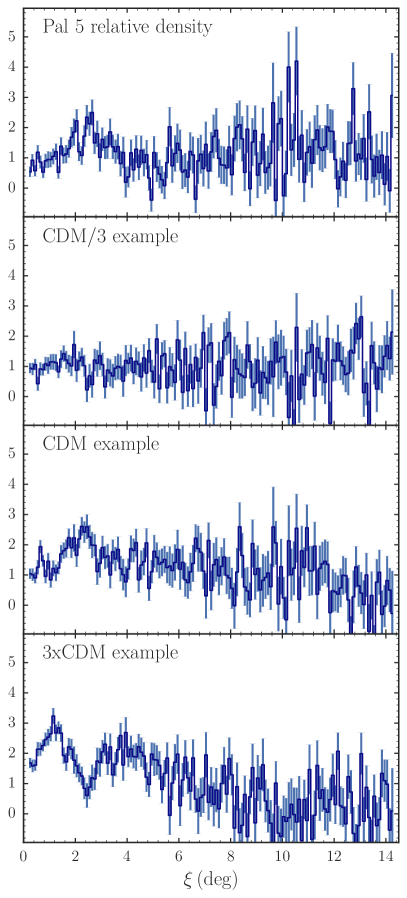
We explore the expected density structure of the Pal 5 stream using simulations of the density using the formalism from this paper in Figure 29. The top panel repeats the normalized observed density and the remaining panels display example simulations of impacts with masses between $10^{6}\,\mathrm{M}_{\odot}$ and $10^{9}\,\mathrm{M}_{\odot}$ for different impact rates, with the fiducial CDM rate of 42.9 impacts corresponding to 42.54 subhalos in this mass range within $25\,\mathrm{kpc}$ from the center (see $\mathsection$ 2.3). Because we can currently only measure the largest-scale density fluctuations, we include impacts up to $X=10$ to include the effect of distant fly-bys. Gaussian noise has been added according to the observational uncertainties. It is clear that the density data, even with the current large uncertainties, holds information on the number of encounters with dark–matter subhalos that the Pal 5 stream has experienced over its lifetime. If the rate is three times less than the fiducial CDM rate—as is predicted from simulations that model the disruption of subhalos by the Milky Way’s disk (D’Onghia et al., 2010)—essentially no intrinsic density perturbations are induced above the noise. If the rate is three times higher than the fiducial CDM rate, large-scale density features become apparent. Simulations for the CDM rate often give a good match to the observed data, as exemplified by the example shown.

Figure 30: Power spectrum of Pal 5. The black points display the power spectrum of the relative density along the trailing arm of Pal 5 (bottom panel of Figure 28) after subtracting the approximate noise level ($\approx 0.3$; points below or just above this level are indicated as upper limits); the gray line shows the noise power spectrum based on the median uncertainty. The colored curves display the median density power spectra of simulations with different subhalo-encounter rates. The gray band shows the interquartile range for simulations with the fiducial CDM rate. Pal 5’s observed power on the largest scales is consistent with the power induced by a CDM-like population of dark–matter subhalos; it is inconsistent with much higher rates.

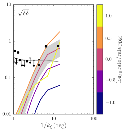
The density power spectrum of the Pal 5 stream is displayed in Figure 30. This figure shows an estimate of the intrinsic power spectrum, subtracting off the median power spectrum from simulations of the noise. On scales $\lesssim 5^{\circ}$, the power spectrum is consistent with the noise, but the Pal 5 data display excess power on scales larger than five degrees. This figure also displays median density power spectra for simulations with different rates of impacts. As expected from Figure 29, rates below the CDM rate only produce power below the noise level, while rates a few times larger than the CDM rate produce more power than is observed. Similar to the GD-1-like example in $\mathsection$ 4 above, very high impact rates again lead to a smoother stream, because most of the stream becomes very low in surface brightness. As discussed above, the power on the largest scales is significantly affected by the density-normalization procedure and should not be trusted too much.

To determine a rigorous constraint on the number of subhalos near Pal 5’s orbit, we use Approximate Bayesian Computation (ABC) to construct an approximation to the posterior probability distribution (PDF) of the rate of impacts (Marin et al., 2012). ABC approximates the PDF of the rate based on the Pal 5 density data without evaluating a likelihood function, but rather using simulations of the density, which we can easily produce using our formalism. ABC works by drawing a rate from the prior distribution of the rate, which we choose to be uniform in $\log_{10}$ of the rate between CDM/10 and 10xCDM, and simulating the observed relative density for this rate. ABC then constructs the PDF by keeping only those simulations that are within a certain tolerance of the real data or a set of summaries of the real data. Ideally, data summaries are sufficient statistics for the inference in question; summary statistics that are not sufficient will create wider PDFs, because they do not make full use of the data. As the data summaries, we use the power $\sqrt{\delta\delta}$ on the three largest observed scales and the bispectrum on the second largest scale, because these are the only scales on which the power and the bispectrum can be measured from the current data (e.g., Figure 30; the power on the third largest scale is $\approx 0.05$, but shown as an upper limit at the noise level in this figure). We keep those simulations that (a) match the power on the largest scale to within 1.5 (loose, to account for the effect of the density normalization, see below), (b) the power on the second-largest scale to within 0.15, (c) the power on the third-largest scale to within 0.2, and (d) match the bispectrum at $6.5^{\circ}$ (specifically, $B(1/6.5^{\circ},1/6.5^{\circ})$) to within 0.03 (for both the real and imaginary part). The tolerances on the power on the second- and third-largest scales and on the bispectrum are approximately as small as makes sense given the noise in the data and the observed power; the power spectrum and the bispectrum on smaller scales are too noisy to lead to a useful constraint. The resulting PDFs do not depend on the exact values of the tolerances. Because the most time-consuming part of the simulations is computing the relative densities, we perform 100 simulations of the noise for each rate (a sort of Rao-Blackwellization). That is, we produce 100 simulations for each rate by adding 100 realizations of the noise to each relative-density realization.

Figure 31: Posterior probability distribution functions for the rate of dark–matter subhalo encounters based on Pal 5 data. The PDFs are obtained by using simulations of Pal 5 and ABC to match the power on the three largest scales in Figure 30 and to match the bispectrum at $6.5^{\circ}$. Different curves include impacts in different mass ranges; they converge below $10^{7}\,\mathrm{M}_{\odot}$. The current Pal 5 data prefer a rate of impacts equal to or smaller than that predicted by CDM. The data are inconsistent with high impact rates. The data are sensitive to subhalos with masses down to $\approx 10^{6.5}\,\mathrm{M}_{\odot}$.

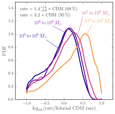
The PDF produced by this procedure including impacts in different mass ranges is displayed in Figure 31. Simulations of impacts of a single mass with the CDM rate expected for the surrounding mass decade (e.g., that of $10^{6}\,\mathrm{M}_{\odot}$ to $10^{7}\,\mathrm{M}_{\odot}$ for $M=10^{6.5}$; cf. Figure 12) indicate that we should be sensitive down to $\approx 10^{6.5}\,\mathrm{M}_{\odot}$. This is borne out by the PDFs for simulations with masses between $10^{x}\,\mathrm{M}_{\odot}$ and $10^{9}\,\mathrm{M}_{\odot}$, which converge for $x$ between 6 and 7. The PDF peaks at a rate that is $1.4^{+1.6}_{-0.9}\times$CDM or that has $10^{+11}_{-6}$ dark–matter subhalos with masses between $10^{6.5}\,\mathrm{M}_{\odot}$ and $10^{9}\,\mathrm{M}_{\odot}$ within $20\,\mathrm{kpc}$ from the Galactic center (Pal 5’s approximate apocenter). The $95\,\%$ upper limit is $3.2\times$CDM or 23 subhalos within the central $20\,\mathrm{kpc}$; the $99\,\%$ limit is $4.2\times$CDM. This conversion between rate relative to CDM and number of subhalos uses the expected CDM rate from the Via Lactea II simulation (Diemand et al., 2008), but the number is what we directly measure. The CDM rate computed from the Aquarius simulations (Springel et al., 2008) for a $M=10^{12}\,\mathrm{M}_{\odot}$ Milky Way halo is about twice that from Via Lactea II (see Erkal et al. 2016); interpreted using the Aquarius simulations, our number measurement would correspond to $0.7^{+0.8}_{-0.5}\times$CDM. Both rates are clearly consistent with CDM. Expressed as a mass fraction $f_{\mathrm{sub}}$ in subhalos for a total halo mass within 20 kpc of $\approx 10^{11}\,\mathrm{M}_{\odot}$ (Bovy & Rix, 2013), our result is $f_{\mathrm{sub}}(r<20\,\mathrm{kpc})\approx 0.2\,\%$ for $M=10^{6.5}\,\mathrm{M}_{\odot}$ to $10^{9}\,\mathrm{M}_{\odot}$.

The PDF based on the bispectrum alone is almost the same as that shown in Figure 31 and the bispectrum is thus fully consistent with the power spectrum. This demonstrates the power of the bispectrum. While the data are most compatible with a rate around the fiducial CDM rate, we cannot rule out a much lower rate, such as that expected from the depletion of dark–matter subhalos by the massive Milky Way disk. We have repeated the analysis for impacts with masses between $10^{6}\,\mathrm{M}_{\odot}$ and $10^{9}\,\mathrm{M}_{\odot}$ using different order polynomials to normalize Pal 5’s density. For linear or quadratic normalizations, the PDF shifts by $\approx 0.5\sigma$ and is essentially the same as that for masses between $10^{7}\,\mathrm{M}_{\odot}$ and $10^{9}\,\mathrm{M}_{\odot}$ in Figure 31. Therefore, the normalization has only a marginal effect for the current data. We have repeated these tests for the mock data analyzed in Appendix D. The mock data display similar behavior to the real data, lending further support to our inferential procedure.

As discussed in $\mathsection$$\mathsection$ 4 and 5, the rate of impacts inferred from observations of the power spectrum and bispectrum is likely to be degenerate with the assumed age of the stream. To investigate how this affects the analysis of the Pal 5 data, we have repeated the inference in this section for Pal-5 stream ages of $3\,\mathrm{Gyr}$ and $10\,\mathrm{Gyr}$. For these ages the peak of the rate PDF shifts to $\approx 4\times$CDM and $\approx 0.25\times$CDM, respectively. As expected, there is no preference for any of the ages. We do not consider $3\,\mathrm{Gyr}$ to be a plausible age for the Pal 5 stream, because Küpper et al. (2015) found an age of $3.4\,\mathrm{Gyr}$ for the segment of the stream that they extracted from the SDSS footprint and the data from Ibata et al. (2016) trace the stream a few degrees further, requiring an age of at least $4\,\mathrm{Gyr}$. We thus consider the measurement of the rate quoted above to be a good upper limit. Nevertheless, marginalizing over all three considered ages by assuming (for simplicity) that any of these ages are a priori equally probable produces a rate PDF that is approximately flat up to $\approx 3\times$CDM and has a $95\,\%$ upper limit of $5\times$CDM.

We can confidently rule out very large rates of impacts corresponding to substructure that is $\gtrsim 5$ times more abundant than expected from CDM simulations. However, there are effects that we have ignored in our analysis. We have assumed a constant background level in determining the Pal 5 density and have disregarded potential density fluctuations due to variable extinction. We have further assumed a constant stripping rate in our model, rather than concentrating stripping episodes near pericentric passages. Simulations using the formalism of Bovy (2014) and Sanders (2014), but concentrating $73\,\%$ of the stripping at pericentric passages induce power on the largest scales that is $<0.1$, far below the noise and data level (see Figure 30). This demonstrates that pericentric stripping plays an unimportant role in the density structure of the Pal 5 stream (see also Dehnen et al. 2004). We have assumed a rather low velocity dispersion for the population of dark–matter subhalos of $\sigma_{h}=120\,\mathrm{km\ s}^{-1}$. And we have ignored the contribution from giant molecular clouds (GMCs), the largest of which may act much like dark–matter subhalos. However, there are very few GMCs with $M\gtrsim 10^{6.5}\,\mathrm{M}_{\odot}$ in the inner Milky Way and practically none within Pal 5’s orbital volume (Rosolowsky, 2005); a close enough encounter with even a single massive GMC is unlikely to have occurred. All of these effects except for the age would (effectively) increase the power in the model and thus reduce the inferred rate. Therefore, the measurement here provides a robust upper limit on the rate of impacts. Appendix D tests the procedure from this section further using mock $N$-body realizations of perturbed Pal-5-like streams. These tests demonstrate that our procedure recovers the correct rate for a a Pal-5-like stream perturbed by a realistic subhalo population.

$\mathsection$ 8 Discussion

In this paper we have introduced a novel calculus for computing the effect of encounters with dark–matter subhalos on tidal streams and we have discussed the perturbations to the density and track location that they induce. In this section, we discuss various aspects of the approximations that we have made, new insights on how to determine the presence of subhalo impacts, and the prospects for observationally measuring the power spectra and bispectra that we have computed.

Episodic stripping and epicyclic motions: All of the simulations in this paper use a constant stripping rate to create the unperturbed stream model. Realistic streams are probably better modeled including a component of stripping at pericentric passages and may have correlations between the actions and angles upon exiting the progenitor that lead to intricate epicyclic motions (e.g., Küpper et al., 2010, 2012). These effects can be easily incorporated into the fast line-of-parallel-angle approach presented here. The line-of-parallel-angle approach provides a fast way to relate a present-day $(\mathbf{\Omega},\boldsymbol{\theta})$ to the $\mathbf{\Omega}$ at stripping ($\Delta\theta_{\parallel}=0$) and does not depend on a particular form of the initial distribution of frequency–angle offsets from the progenitor or of the stripping times. Any initial distribution of $\mathbf{\Omega}$ and $\theta_{\perp}$ can be evaluated with any stripping time distribution $p(t_{s})$; we chose to work with a constant stripping rate because it is the easiest case. Because of mixing within the stream, episodic stripping will only significantly affect the youngest part of the stream, that is, the part closest to the progenitor, while the subhalo impacts mostly affect the oldest part of the stream (see also Ngan & Carlberg 2014). Density and track variations due to subhalo impacts and episodic stripping will also be largely uncorrelated and thus add up independently in the power spectrum. Thus, we expect that episodic stripping is of minor importance in constraining the subhalo mass spectrum and that density–track cross power spectra and the bispectrum can distinguish between these two effects.

The impulse approximation: All of our calculations use the impulse approximation to determine the velocity kicks due to a dark–matter subhalo fly-by. However, the impulse approximation may not hold for all impact geometries or if the dark–matter subhalos are in the process of being disrupted (Bovy, 2016). In the linear approximation where the effect of all impacts can be computed based on the unperturbed stream track, velocity kicks could be computed accounting for the full trajectory of the subhalo and then converted to frequency–angle coordinates. This would increase the computational cost, but only marginally because the effect of the fly-by could still be computed along a one-dimensional approximation to the stream as the stream will still be perturbed coherently at a given $\Delta\theta_{\parallel}$. Further investigation of the impulse approximation and when it breaks down is warranted for getting precise measurements of the subhalo mass function. However, the details of the interaction are largely unimportant, because the $\delta\Omega_{\parallel}^{g}$ kicks dominate the late-time effects of subhalo encounters and these kicks are mainly determined by the overall amplitude and spatial scale of the impacts; they care little about the details of the velocity kicks.

Tidal streams as corrugated sheets: To a first approximation a tidal stream is a one-dimensional object along the $\Delta\theta_{\parallel}$ direction in six-dimensional phase–space. To a second approximation, a stream is a two-dimensional sheet in $(\Delta\theta_{\parallel},\Delta\Omega_{\parallel})$. For cold streams originating from globular-cluster progenitors, the extent of a stream in the remaining four phase–space dimensions is negligible and will likely not be observable in the coming decades. This follows from the structure of phase–space near the orbit of a tidal stream: the largest eigenvalue of the Hessian matrix $\partial\mathbf{\Omega}/\partial\mathbf{J}$ is typically a factor of $\approx 30$ larger than the second largest eigenvalue (Sanders & Binney, 2013). The same Hessian controls the effect of subhalo encounters: any small perturbation to a stream primarily affects the parallel direction $\Delta\Omega_{\parallel}$ by the same factor (see, for example, Figure 5 and the parallel-only models in Appendix A). Thus, subhalo kicks turn a tidal stream from a smooth sheet into a corrugated sheet, but the overall dimensionality remains two. At a given position along a stream, the stream is therefore one dimensional. This implies that all projections of the stream are almost exactly correlated. That is, perturbations due to subhalo kicks in the sky location, distance, and velocity of a stream are entirely correlated. The amplitude of the deviations in different coordinates is different (and may have a smooth trend along the stream if the stream does not follow an orbit), but the shape is the same. This means that we can combine different projections to better measure track deviations and that we can use cross-correlations between different projections to clean the signal from background contamination, extinction variations, or any part of the signal that is not intrinsic to the stream. Data are already nearly good enough that cross-correlations between the density and track could be informative. It is imperative that we start measuring the track of tidal streams in detail now.

Using the density or track to measure the subhalo mass function: We have computed the effect of subhalo impacts on both the density and the track of a tidal stream. It is clear from the power spectrum that the density is a more sensitive tracer: fluctuations in the density are larger than those in the track and are easier to measure. This is because density perturbations build up over time, while track perturbations start out large at the time of impact and then fade because material streams away from the impact point and because of internal mixing. However, this sensitivity comes at a price. Density perturbations do not typically respond linearly to increases or decreases in the rate of impacts (e.g., Figures 15 and 16). The track deviations do largely respond linearly, as if they all add up independently of each other. Track deviations are therefore a much more well-behaved tracer of the rate of impacts. However, Figures 21 and 22 demonstrate that the track power spectrum will be difficult to observe, especially for $M\lesssim 10^{6.5}\,\mathrm{M}_{\odot}$. The cross power spectrum of the density and track is therefore the best compromise between sensitivity and well-behavedness. Density fluctuations due to subhalos confirmed through the cross power spectrum with a track projection will make for a compelling case for cold dark–matter structure.

Scale dependence of fluctuations: One of the main advantages of the line-of-parallel-angle approach for computing the effect of subhalo impacts over direct simulations or using tracer particles is its ability to make noiseless predictions for the structure of streams (that is, Poisson noise in the particle distribution in $N$-body simulations is absent). This allows us to trace the induced structure on very small scales. Previous work has claimed that structure on scales smaller than a few times the width of a tidal stream is suppressed (e.g., Carlberg, 2013). We find no evidence for this here. For the GD-1-like stream considered here, we find structure on scales a few times the width of the stream. The only cut-off that is induced is due to a cut-off in the subhalo mass function (see Figure 15).

Heating of tidal streams: Much of the early work on the effect of subhalo encounters on tidal streams focused on the increase in the velocity dispersion of the stream (e.g., Johnston et al., 2002; Ibata et al., 2002; Carlberg, 2009). Large effects were found because these studies significantly overestimated the number of subhalos present in the inner Milky Way. We have focused on the mean stream track rather than its dispersion. It is clear that the velocity dispersion of a perturbed stream could be computed using a similar approach as that in $\mathsection$ 3.3. It is unclear whether this will be a useful exercise, especially if one is interested in subhalos with masses $<10^{7}\,\mathrm{M}_{\odot}$. These induce very little increase in the dispersion that would be largely swamped by the increase because of higher-mass encounters. Increases in dispersion are also much more difficult to measure observationally.

The importance of small scales: We have analyzed the density of the Pal 5 stream in $\mathsection$ 7 above. Because of the large uncertainties, we were only able to use the largest scales. These are dominated by large subhalo masses $M\gtrsim 10^{7}\,\mathrm{M}_{\odot}$, which are most susceptible to modeling errors such as the breakdown of the impulse approximation and the maximum impact parameter, and these scales are also strongly affected by uncertainties in the smooth stream model. All of these problems become much less important on smaller scales, which also allow the more interesting mass range $M\lesssim 10^{7}\,\mathrm{M}_{\odot}$ to be accessed. Thus, a high priority for this field is to push density and track measurements to few degree scales. Made-to-order modeling for potential observational targets like GD-1 is necessary to establish the optimal strategy, but a focus on some parts of a stream with sparse sampling of the full stream to constrain the unperturbed-stream model and to access larger-scale modes is likely to be a good way forward.

Statistical versus direct measurements of impacts: We have focused in this paper on predicting the statistical properties of the fluctuation pattern of the density and track of perturbed tidal streams. However, with good phase–space measurements individual impacts may be fully characterized in terms of mass, fly-by velocity, impact parameter, etc., especially at the high-mass end (e.g., Erkal & Belokurov, 2015b). It is clear that the fast line-of-parallel-angle algorithm developed here can also be used in fitting the parameters of a single impact or multiple impacts, because it computes the full density and track structure in configuration space that can be compared to observational data. This may prove to be useful in two ways: (a) fitting single impacts to find evidence of individual low-mass dark–matter subhalos, improving on the method of Erkal & Belokurov (2015b) by accounting for the eccentricity and internal dispersion of tidal streams; and (b) fast fitting of a small number of impacts that induce the largest changes in a tidal stream and subtracting their effect to reveal the statistical fluctuations due to lower-mass subhalos. Point (b) will make it easier to detect $M<10^{6}\,\mathrm{M}_{\odot}$ subhalos, because it would allow their statistical effect to be seen on the larger scales where they induce more power (cf. Figure 20).

Observational requirements to observe $10^{5}\,\mathrm{M}_{\odot}$ subhalos: The density power spectra and density–track cross power spectra in observable coordinates in Figures 20 and 24 make it clear that we can determine the abundance of $10^{5}\,\mathrm{M}_{\odot}$ dark–matter subhalos in the Milky Way’s halo, if we can measure the scale dependence of the power down to few degree scales for a few long, cold tidal streams such as GD-1. While this prediction is somewhat on the optimistic side (the GD-1-like stream is at the cold, old side of what is expected for a stream like GD-1) and it is by no means clear that GD-1 will be the best target for such studies, this prospect makes a compelling case for pursuing better measurements of the density and track of cold tidal streams.

The observational uncertainties in Figures 20 and 24 correspond to $10\,\%$ density measurements in $0.3^{\circ}$ bins along the stream. For GD-1, which has a stellar mass of $\approx 20,000\,\mathrm{M}_{\odot}$ (Koposov et al., 2010), this would require a background-free map of about half of all of the stars down to the bottom of the main-sequence. While this may seem unrealistic, a wide-field proper motion survey with WFIRST or a wide-field AO imager on a large telescope may get close to this goal in ten years from now. Until then and because background contamination is the biggest issue limiting the current measurements (see the analysis of Pal 5 above), a line-of-sight velocity survey of GD-1 or a similar stream may be the best way forward. A line-of-sight velocity precision of $\lesssim 10\,\mathrm{km\ s}^{-1}$ would significantly reduce the background from halo stars, especially when combined with abundance information from the spectra. GD-1 has approximately 3,000 stars down to $r=22$ (Koposov et al., 2010). A background-free map of those would allow $25\%$ density measurements, which would still allow the contribution of $\approx 10^{5.5}\,\mathrm{M}_{\odot}$ subhalos to be seen in the density (see Figure 20). Observing all stream members down to $r=24$ would essentially bring the noise level down to that in Figure 20. This will not be easy and GD-1 might not be the best target, but investing in this will help settle the question of whether dark–matter clumps on scales smaller than those of galaxies.

It is clear from Figures 21 and 23 that measuring deviations in the track of a stream using the line-of-sight velocity will be a frustrating experience. The predicted deviations are $<1\,\mathrm{km\ s}^{-1}$ from the largest impacts and $<0.1\,\mathrm{km\ s}^{-1}$ from lower-mass subhalos. We have not shown the predicted power spectra for the proper motions, because they are far beyond what can be measured. While line-of-sight velocity measurements can be helpful on the largest scales corresponding to $\gtrsim 10^{7}\,\mathrm{M}_{\odot}$ subhalos, their main use will be in removing background contamination. This is simply a reflection of the fact discussed above that track deviations at a given distance along the stream are one-dimensional: every projection measures the same deviation and this is much easier to observe in sky position and distance than velocity.

$\mathsection$ 9 Conclusion

In this paper we have developed a novel method for computing the phase–space structure of tidal streams perturbed by dark–matter subhalo impacts. We have used it to study the fluctuations in the density and location (the “track”) of a stream due to subhalo impacts with different overall rates and masses. We have also performed a first rigorous measurement of the abundance of dark–matter subhalos with $M\gtrsim 10^{6.5}\,\mathrm{M}_{\odot}$ within about $20\,\mathrm{kpc}$ from the center of the Milky Way using density data for the Pal 5 stream. Our main findings and conclusions are the following:
$\bullet$ The line-of-parallel angle approach to compute the phase–space structure of a tidal stream developed in $\mathsection$ 3.3 is a fast method to compute the effect of subhalo impacts, allowing the perturbed structure of a tidal stream for a given, realistic set of impacts to be computed in a matter of minutes. We have made a number of assumptions in this approach and its application in this paper, but most of these are not of fundamental importance to the speed of the method. The basic assumption that allows the fast computation is that of the linearity of the impacts, i.e., that we can compute the velocity kicks for all kicks based on the unperturbed stream track, rather than the perturbed stream track. We have extensively tested this assumption in Appendix A and find it to work well, especially for the relatively low number of impacts expected for a CDM-like population of subhalos in the inner Milky Way. Other assumptions, such as the validity of the impulse approximation, our ignoring of kicks in the perpendicular frequency and angle directions, and the specific assumptions made about the initial frequency distribution of the tidal debris and the rate at which material is stripped are not essential to the method and could be easily relaxed at little additional computational cost.
$\bullet$ Tidal streams, when perturbed by a population of subhalo impacts, are unlikely to display clearly identifiable gaps in their density profiles (see, e.g., Figure 10), even when the number of impacts is relatively small and especially for those gaps that are due to low-mass subhalos ($M\lesssim 10^{7}\,\mathrm{M}_{\odot}$). But the subhalo impacts induce a rich structure of fluctuations on different scales that can be observed through the power spectrum of the density and track. The structure in the density and that in the track are strongly correlated—indeed, it is the structure in the track that gives rise to the density fluctuations at later times. Because cold–dark–matter subhalos follow a somewhat tight concentration–mass relation, different mass subhalos give rise to structure on different scales, with smaller scales dominated by very low-mass subhalos ($M\lesssim 10^{7}\,\mathrm{M}_{\odot}$). Observations of this power spectrum in the density and track, of its scale dependence, and of the cross-correlation between the density and track and of different projections of the track are a clear path forward to determining the subhalo mass spectrum between $10^{5}\,\mathrm{M}_{\odot}$ and $10^{9}\,\mathrm{M}_{\odot}$ from observations of tidal streams in the Milky Way. Going beyond the power spectrum, the time dependence of the impact rate and of the evolution of density fluctuations induces significant higher-order moments such as can be observed through the bispectrum that may be observable in future data and that would constitute a powerful confirmation of the subhalo-impact origin of density and track fluctuations.
$\bullet$ Using this new framework, we have performed the first rigorous inference of the dark–matter subhalo population using data on the density of the Pal 5 stream. We find a rate of impacts that is $1.4^{+1.6}_{-0.9}\times$CDM, equivalent to $10^{+11}_{-6}$ dark–matter subhalos with masses between $10^{6.5}\,\mathrm{M}_{\odot}$ and $10^{9}\,\mathrm{M}_{\odot}$ within $20\,\mathrm{kpc}$ from the Galactic center or a subhalo mass fraction of $f_{\mathrm{sub}}(r<20\,\mathrm{kpc})\approx 0.2\,\%$ over the same mass range. While the uncertainty on the rate is large and this measurement comes with caveats because we can only use the power on the largest scales given the current observational uncertainties and because of the uncertainty on the Pal 5 stream’s age, this constraint is already at an interesting level and the upper limit in particular is robust. Furthermore, simulations of the structure in the Pal 5 stream induced by a CDM-like population of subhalos (see Figure 29) provide a remarkable match to the observed density profile. This first analysis makes it clear that modest improvements in the data quality will soon lead to the best available constraints on the low-mass subhalo population of a Milky-Way-sized halo, especially if we can push the analysis to smaller scales.

All code used in this paper is made publicly available, except for the GADGET-3 code used to run the $N$-body simulations, as we are not at liberty to release this. The methods from $\mathsection$ 3 are contained in galpy for the case of a single impact (galpy.df.streamgapdf) and as the galpy extension galpy.df.streampepperdf for the case of multiple impacts. All of the analysis in this paper can be reproduced using the code found at

https://github.com/jobovy/streamgap-pepper

.

Acknowledgments We thank the anonymous referee for a constructive report. This research received financial support from the Natural Sciences and Engineering Research Council of Canada. The research leading to these results has received funding from the European Research Council under the European Union’s Seventh Framework Programme (FP/2007-2013)/ERC Grant Agreement no. 308024.

Appendix A Detailed tests of the frequency–angle framework with $N$-body simulations

Figure 32: Comparison between an $N$-body simulation of an impact with a $10^{7}\,\mathrm{M}_{\odot}$ subhalo (black points) and mock data generated from the modeling in frequency–angle space. The red points are for the generative model in which kicks $(\delta\mathbf{\Omega}^{g},\delta\boldsymbol{\theta}^{g})$ in all coordinates are included, the yellow points are for the case where only $\delta\Omega_{\parallel}^{g}$ kicks in the parallel frequency direction are applied. The phase-space differences are shown as a function of unperturbed $x$ position (that in the absence of the impact) near the current location of the impact point, which is known in both the simulation and the mock data. As expected from the phase–space structure near the stream, most of the effect of the subhalo is in the parallel direction and the yellow, red, and black points almost completely overlap (both in their mean trend and their scatter at a given $x$). Our frequency–angle-with-impulsive-kicks modeling produces a configuration-space phase-space structure that agrees with the $N$-body simulation.

Figure 33: Same as in Figure 32, but for an impact with a $10^{5}\,\mathrm{M}_{\odot}$ subhalo. The impact induces configuration-space deviations on the order of $100\,\mathrm{pc}$ and $50\,\mathrm{m\,s}^{-1}$. The agreement between the $N$-body model and the data generated from the frequency–angle modeling is excellent.

Figure 34: Like Figure 32, but for a simulation where the stream has been perturbed by two $10^{8}\,\mathrm{M}_{\odot}$ subhalos at nearly the same location along the stream separated by $1\,\mathrm{Gyr}$ in time and observed $1\,\mathrm{Gyr}$ after the second impact (see text for the exact setup). The phase-space differences are shown as a function of unperturbed $y$ position near the current location of the impact points. The agreement between the $N$-body simulation and the frequency–angle modeling is good, with only minor differences (note that the $y$-range in the middle, lower panel is much smaller than those in the left and right lower panels).

Figure 35: As Figure 34, but for the case where the second impact is that of a $10^{7}\,\mathrm{M}_{\odot}$ subhalo.

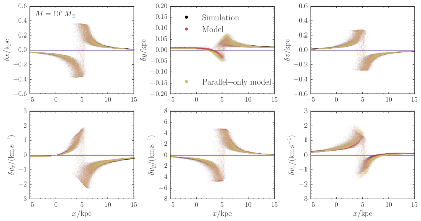
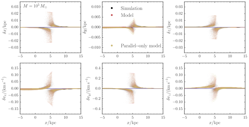
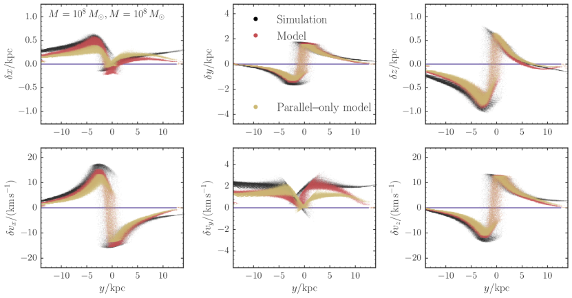
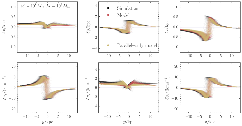
In this Appendix, we investigate the applicability of our stream-gap-modeling framework in frequency–angle space by comparing to full $N$-body simulations of the interaction between dark–matter subhalos and stellar streams. These tests are similar to those described by Sanders et al. (2016). There, a detailed comparison between the frequency–angle framework for a single impact with a $10^{8}\,\mathrm{M}_{\odot}$ subhalo and a cold stellar stream was presented in configuration space. To as closely follow the $N$-body simulation of the stream as possible, a custom unperturbed stream model was constructed that combines stripping events at pericenter with a contribution from a continuous stripping process; the combination matches the simulation of the unperturbed stream. This allowed a fair comparison between the frequency–angle framework for applying subhalo kicks ($\delta\mathbf{\Omega}^{g},\delta\boldsymbol{\theta}^{g})$. Good agreement between the frequency–angle framework and the $N$-body simulation of the interaction was found.

Here, we are interested in testing various additional aspects of our framework. First and foremost is whether the framework remains accurate down to the lowest-mass subhalos that we consider in this paper ($M=10^{5}\,\mathrm{M}_{\odot})$. Additionally, we want to test the accuracy of our approximation that all kicks $(\delta\mathbf{\Omega}^{g},\delta\boldsymbol{\theta}^{g})$ are computed on the basis of the unperturbed stream track (i.e., that the effect of the kicks is linear at the time of impact). Lastly, we want to explicitly test the approximation used in the fast line-of-parallel-angle approach that the main effect of subhalo impacts is in the parallel frequency direction, such that we only need to consider $\delta\Omega_{\parallel}^{g}$.

We test that our framework works down to $M=10^{5}\,\mathrm{M}_{\odot}$ by repeating the simulations in Sanders et al. (2016) for impacts with $M=10^{7}\,\mathrm{M}_{\odot}$, $10^{6}\,\mathrm{M}_{\odot}$, and $10^{5}\,\mathrm{M}_{\odot}$. These simulations were run with the $N$-body part of gadget-3 which is similar to gadget-2 (Springel, 2005) and are identical to the setup in Sanders et al. (2016). The impact in Sanders et al. (2016) was with a Plummer sphere with $M=10^{8}\,\mathrm{M}_{\odot}$ and $r_{s}=625\,\mathrm{pc}$. For the lower masses, we change the scale radii to $250\,\mathrm{pc}$, $80\,\mathrm{pc}$, and $40\,\mathrm{pc}$, respectively. Otherwise all of the impact parameters (location along the stream, impact parameter [0], fly-by velocity, impact time [$880\,\mathrm{Myr}$ ago]) are the same. We generate mock data from the frequency–angle model (see $\mathsection$ 3.1 and Sanders et al. 2016) in configuration space for both an unperturbed stream and a stream perturbed by a subhalo using the same initial conditions. This way, we can compare the present-day position of each individual mock data point between the perturbed and unperturbed model. These differences in position for all phase–space coordinates in the vicinity of the gap are displayed in Figures 32 and 33 for the $10^{7}\,\mathrm{M}_{\odot}$ and $10^{5}\,\mathrm{M}_{\odot}$ impacts, respectively (red points). The same differences in present-day position for the $N$-body simulation with and without perturbation (starting from the same initial condition) are shown as the black points. The yellow points show the mock data that are generated by only applying the kick in parallel frequency $\delta\Omega_{\parallel}^{g}$, that is, without applying kicks in the perpendicular direction and without any angle kicks. All three simulations agree, demonstrating that our frequency–angle-with-impulsive-kicks framework works well down to $M=10^{5}\,\mathrm{M}_{\odot}$ (the $M=10^{6}\,\mathrm{M}_{\odot}$ comparison is similar, but not shown here). This is especially impressive considering that the effect of the kicks is accurately modeled at the few pc and $50\,\mathrm{m\,s}^{-1}$ level for the lowest-mass interaction. That the model that only considers $\delta\Omega_{\parallel}^{g}$ kicks agrees with the full model shows that this approximation that we make throughout most of this paper is valid.

Figure 36: Like Figure 32, but for a simulation where the stream has been perturbed by 24 subhalos with masses between $10^{6}\,\mathrm{M}_{\odot}$ and $10^{8}\,\mathrm{M}_{\odot}$ that impact the stream between $10\,\mathrm{Gyr}$ and $11.75\,\mathrm{Gyr}$ and that are otherwise sampled using the method in $\mathsection$ 2.3. The phase-space differences are shown at $12\,\mathrm{Gyr}$ as a function of unperturbed azimuth $\phi$ position all along the trailing arm of the stream. The agreement between the $N$-body simulation and the frequency–angle modeling is good, with only a small overall offset in $y$, $v_{x}$, and $v_{y}$.

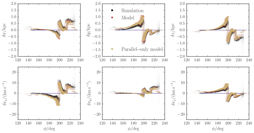
To further stress-test our framework, we have also run $N$-body simulations where the same part of the stream gets impacted by two massive dark–matter subhalos. We impact the same stream as in Sanders et al. (2016) again at $10\,\mathrm{Gyr}$ with the same $10^{8}\,\mathrm{M}_{\odot}$ impact as in Sanders et al. (2016) (except that it has $r_{s}=1.05\,\mathrm{kpc}$ to more closely follow the expected mass–concentration relation), but follow it with another impact in almost the same part of the stream at $11\,\mathrm{Gyr}$ (the mass of this second impact is either $10^{8}\,\mathrm{M}_{\odot}$ or $10^{7}\,\mathrm{M}_{\odot}$). The second impact is again a direct impact and it has a fly-by velocity of $100\,\mathrm{km\ s}^{-1}$ pointed along the $x$ direction; the $10^{7}\,\mathrm{M}_{\odot}$ subhalo has $r_{s}=332\,\mathrm{pc}$. We compare configuration space differences in all coordinates $1\,\mathrm{Gyr}$ after the second impact for both of these setups. These results are displayed in Figures 34 and 35. While the agreement between the frequency–angle models and the $N$-body simulations is not perfect, it is clear that the model overall does a good job of matching the effects seen in the $N$-body simulation.

This two-impact comparison that we have performed here is in many ways a worst-case scenario for our framework, because it has multiple large impacts happen in almost the same part of the stream. Because large impacts are rare, this should not happen often in reality. As the ($10^{8}\,\mathrm{M}_{\odot},10^{7}\,\mathrm{M}_{\odot}$) demonstrates, a large direct impact followed by a smaller direct impact is already much better modeled than that of two $10^{8}\,\mathrm{M}_{\odot}$ subhalos, and even such combinations are rare. Therefore, we are confident that our framework correctly captures the effect of multiple impacts.

As a final test, we sample 24 fly-bys with masses between $10^{6}\,\mathrm{M}_{\odot}$ and $10^{8}\,\mathrm{M}_{\odot}$ that impact the trailing part of the same stream between $10\,\mathrm{Gyr}$ and $11.75\,\mathrm{Gyr}$ and we observe the stream again at $12\,\mathrm{Gyr}$. The parameters describing these impacts are sampled using the statistical procedure of $\mathsection$ 2.3 (the CDM-like rate for this setup is 21.5 expected impacts). The set of fly-bys has three impacts with $M\approx 3\times 10^{7}\,\mathrm{M}_{\odot}$ and many lower-mass impacts. The phase–space differences at the present time as a function of Galactocentric azimuth are displayed in Figure 36. These differences are dominated by a single large perturbation due to one of the $M\approx 3\times 10^{7}\,\mathrm{M}_{\odot}$ fly-bys, but have much structure on smaller scales as well due to the other 23 fly-bys. The frequency–angle model matches the overall structure of the phase–space differences and also reproduces most of the smaller-scales wiggles. There is a slight $\approx$constant offset in some of the coordinates that may be due an imperfect translation of our modeling setup to the $N$-body code, a breakdown of the impulse approximation, or the slight difference in the stripping rate between the simulation and the model. Close to the progenitor—located around $\phi=240^{\circ}$—the simulation and the model also display some differences, because the details of the stripping rate matter more there than elsewhere and we only roughly match the stripping rate in the model.

Figure 37: Comparison between the relative perturbed/unperturbed density for the $N$-body simulation and frequency–angle model in Figure 36 (blue and orange curves, respectively). The 24 subhalo impacts with masses between $10^{6}\,\mathrm{M}_{\odot}$ and $10^{8}\,\mathrm{M}_{\odot}$ create 5 visible gaps that are reproduced by the model, albeit imperfectly. The density power spectra of both curves (not shown) display good agreement.

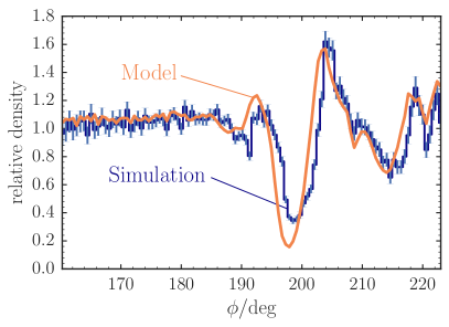
The difference between the relative density (perturbed/unperturbed) between the $N$-body simulation and the model is displayed in Figure 37. The 24 impacts lead to 5 visible gaps in the relative density. All of these are reproduced by the model. The width of the gaps is very well matched, while the depth and the exact location are less well modeled, due to the same reasons that produce the $\approx$constant offset in the phase–space differences. The power spectra of the relative density of the simulation and the model are in good agreement; thus we certainly match the statistical properties of the stream. In all of these comparisons the model that only applies the $\delta\Omega_{\parallel}^{g}$ kicks produces the same results as the model that applies the full $(\delta\mathbf{\Omega}^{g},\delta\boldsymbol{\theta}^{g})$ kicks, demonstrating once again that $\delta\Omega_{\parallel}^{g}$ kicks are all that is necessary to model the effect of subhalo perturbations.

Appendix B Detailed derivation of the line-of-parallel-angle algorithm for multiple impacts

In this appendix, we go through the derivation of the line-of-parallel-angle algorithm in $\mathsection$ 3.3.2 in more detail. We denote the piecewise-polynomial representation of kick $j$ as $\sum_{k}C_{bk}^{j}(\Delta\theta_{\parallel}-x_{b}^{j})^{k}$ for segment $b$, with $j=1$ for the final impact that is undone first. For $\Delta\Omega_{\parallel}\leq\Delta\Omega_{\parallel}^{\mathrm{max}}$ we start by undoing the effect of the final impact as in $\mathsection$ 3.3.1. As in Equation (3.3.1), the point $(\Delta\Omega_{\parallel},\Delta\theta_{\parallel})$ is located at

$$\left(\Delta\Omega_{\parallel}-\sum_{k}C_{bk}^{1}\,\left(\Delta\theta_{\parallel}-\Delta\Omega_{\parallel}\,t_{i}^{1}-x_{b}^{1}\right)^{k},\Delta\theta_{\parallel}-\Delta\Omega_{\parallel}\,t_{i}^{1}\right)\,$$

$$\qquad\qquad\qquad x_{b}^{1}\leq\Delta\theta_{\parallel}-\Delta\Omega_{\parallel}\,t_{i}^{1}<x_{b+1}^{1}\,,$$ (40)

before the final impact. This phase–space point can then be evolved backward until the second-to-last impact at $t_{i}^{2}$. Its frequency remains constant and it arrives at a parallel angle

$$\Delta\theta_{\parallel}-\Delta\Omega_{\parallel}\,t_{i}^{1}$$

$$\qquad-\left(\Delta\Omega_{\parallel}-\sum_{k}C_{bk}^{1}\,\left(\Delta\theta_{\parallel}-\Delta\Omega_{\parallel}\,t_{i}^{1}-x_{b}^{1}\right)^{k}\right)\,(t_{i}^{2}-t_{i}^{1})\,$$

$$\qquad\qquad\qquad x_{b}^{1}\leq\Delta\theta_{\parallel}-\Delta\Omega_{\parallel}\,t_{i}^{1}<x_{b+1}^{1}\,.$$ (41)

Keeping only terms up to linear order in $\Delta\theta_{\parallel}-\Delta\Omega_{\parallel}\,t_{i}^{1}-x_{b}^{1}$, we can re-write this as

$$\Delta\theta_{\parallel}-(t_{i}^{2}-t_{i}^{1})\,\left(-C_{b0}^{1}-C_{b1}^{1}\left[\Delta\theta_{\parallel}-x_{b}^{1}\right]\right)$$

$$\ \ -\Delta\Omega_{\parallel}\,\left(t_{i}^{2}-[t_{i}^{2}-t_{i}^{1}]\,C_{b1}^{1}\,t_{i}^{1}\right)\,,\ x_{b}^{1}\leq\Delta\theta_{\parallel}-\Delta\Omega_{\parallel}\,t_{i}^{1}<x_{b+1}^{1}\,.$$ (42)

If we define

$$\Delta\theta_{\parallel,b}^{2} \equiv\Delta\theta_{\parallel}-(t_{i}^{2}-t_{i}^{1})\,\left(-C_{b0}^{1}-C_{b1}^{1}\left[\Delta\theta_{\parallel}-x_{b}^{1}\right]\right)\,,$$ (43)

$$t^{2}_{b} \equiv t_{i}^{2}-[t_{i}^{2}-t_{i}^{1}]\,C_{b1}^{1}\,t_{i}^{1}\,,$$ (44)

the parallel angle at the time of the second-to-last impact is simply

$$\Delta\theta_{\parallel,b}^{2}-\Delta\Omega_{\parallel}\,t^{2}_{b}\,.$$ (45)

This expression is similar to that for the parallel angle at the final impact (cf. the angle in Equation [B]), except that each segment $b$ now has an individual angle and time associated with it. Previously these were the same ($\Delta\theta_{\parallel}$ and $t_{i}^{1}$) for all segments.

For each segment, we can then undo the kick from the second-to-last impact by determining which segment $b^{\prime}$ $[x_{b^{\prime}}^{2},x_{b^{\prime}+1}^{2}[$ of the second-to-last impact the parallel angle falls in. Undoing the effect of the second-to-last impact then changes the frequency to (from now on we only consider terms up to linear for each kick)

$$\Delta\Omega_{\parallel} -C_{b0}^{1}-C_{b1}^{1}\,\left(\Delta\theta_{\parallel}-\Delta\Omega_{\parallel}\,t_{i}^{1}-x_{b}^{1}\right)$$

$$-C_{b^{\prime}0}^{2}-C_{b^{\prime}1}^{2}\,\left(\Delta\theta_{\parallel,b}^{2}-\Delta\Omega_{\parallel}\,t_{b}^{2}-x_{b^{\prime}}^{2}\right)$$

$$\!\!\!\!\!\!x_{b}^{1}\leq\Delta\theta_{\parallel}-\Delta\Omega_{\parallel}\,t_{i}^{1}<x_{b+1}^{1}\ \mathrm{and}\ x_{b^{\prime}}^{2}\leq\Delta\theta_{\parallel,b}^{2}-\Delta\Omega_{\parallel}\,t_{b}^{2}<x_{b^{\prime}+1}^{2}\,.$$ (46)

We can then run phase–space points backward to the time of the third-to-last impact using this frequency, and similar to Equation (B) we arrive at

$$\Delta\theta_{\parallel,b}^{2}-\Delta\Omega_{\parallel}\,t^{2}_{b}$$

$$\qquad-\left(\Delta\Omega_{\parallel}\right. -C_{b0}^{1}-C_{b1}^{1}\,\left[\Delta\theta_{\parallel}-\Delta\Omega_{\parallel}\,t_{i}^{1}-x_{b}^{1}\right]$$

$$\left.-C_{b^{\prime}0}^{2}-C_{b^{\prime}1}^{2}\,\left[\Delta\theta_{\parallel,b}^{2}-\Delta\Omega_{\parallel}\,t_{b}^{2}-x_{b^{\prime}}^{1}\right]\right)\,(t_{i}^{3}-t_{i}^{2})\,$$

$$\!\!\!\!\!\!\!\!\!\!\!\!\!\!\!\!\!\!\!\!\!\!\!\!\!\!\!\!\!\!\!\!\!\!\!\!x_{b}^{1}\leq\Delta\theta_{\parallel}-\Delta\Omega_{\parallel}\,t_{i}^{1}<x_{b+1}^{1}\ \mathrm{and}\ x_{b^{\prime}}^{2}\leq\Delta\theta_{\parallel,b}^{2}-\Delta\Omega_{\parallel}\,t_{b}^{2}<x_{b^{\prime}+1}^{2}\,.$$ (47)

If we then define

$$\Delta\theta_{\parallel,b}^{3} \equiv\Delta\theta_{\parallel,b}^{2}-(t_{i}^{3}-t_{i}^{2})\,\left(-C_{b0}^{1}-C_{b1}^{1}\left[\Delta\theta_{\parallel}-x_{b}^{1}\right]\right.$$ (48)

$$\quad\qquad\qquad\qquad\qquad\left.-C_{b^{\prime}0}^{2}-C_{b^{\prime}1}^{2}\left[\Delta\theta_{\parallel,b}^{2}-x_{b^{\prime}}^{2}\right]\right)\,,$$

$$t^{3}_{b} \equiv t_{b}^{2}+[t_{i}^{3}-t_{i}^{2}]\,[1+C_{b1}^{1}\,t_{i}^{1}+C_{b^{\prime}1}^{2}\,t_{b}^{2}]\,,$$ (49)

we can again write this angle as

$$\Delta\theta_{\parallel,b}^{3}-\Delta\Omega_{\parallel}\,t^{3}_{b}\,.$$ (50)

Thus, by performing similar operations for all previous impacts, we always keep the same form of expression for the parallel angle of each segment at the previous impact. This is what motivates the updates in Equations (27) and (28) and the definition and updates to $\mathrm{d}\Omega_{b}$, which arise from the need to keep track of all previous changes to the frequency (see Equation [48]).

The discussion so far has not described how the piecewise-linear segments of different impacts mesh throughout the propagation of the line-of-parallel-angle. In Equation (B), we simply wrote the conditions for the parallel angle to be within segments $b$ and $b^{\prime}$ of the last and second-to-last impact. In practice, we can track the segments by re-writing them as segments in present-day $\Delta\Omega_{\parallel}$ rather than $\Delta\theta_{\parallel}$, as done for the case of a single impact in Equation (6). Each previous impact gives rise to a new set of breakpoints in present-day $\Delta\Omega_{\parallel}$ through equations such as Equation (44) and (50). These are computed using Equation (30), where in the notation of this appendix we would have to write $x_{b}^{j}$ instead of $x_{b}$. Because after correcting for the final impact, the expression for the new breakpoints depends on the parameters for each individual segment $b$, for each segment we only add new breakpoints that are within the segment $b$. In Figure 6, the new breakpoints for the second-to-last impact are the small dots that are added to the large dots in the fourth panel.

After correcting for the effect of the third-to-last impact, the frequency becomes (analogous to Equation [B])

$$\Delta\Omega_{\parallel} -C_{b0}^{1}-C_{b1}^{1}\,\left(\Delta\theta_{\parallel}-\Delta\Omega_{\parallel}\,t_{i}^{1}-x_{b}^{1}\right)$$

$$-C_{b^{\prime}0}^{2}-C_{b^{\prime}1}^{2}\,\left(\Delta\theta_{\parallel,b}^{2}-\Delta\Omega_{\parallel}\,t_{b}^{2}-x_{b^{\prime}}^{2}\right)$$

$$-C_{b^{\prime\prime}0}^{3}-C_{b^{\prime\prime}1}^{3}\,\left(\Delta\theta_{\parallel,b}^{3}-\Delta\Omega_{\parallel}\,t_{b}^{3}-x_{b^{\prime\prime}}^{3}\right)$$

$$\!\!\!\!\!\!x_{b}^{1}\leq\Delta\theta_{\parallel}-\Delta\Omega_{\parallel}\,t_{i}^{1}<x_{b+1}^{1}\,,x_{b^{\prime}}^{2}\leq\Delta\theta_{\parallel,b}^{2}-\Delta\Omega_{\parallel}\,t_{b}^{2}<x_{b^{\prime}+1}^{2}\,,$$

$$\mathrm{and}\ x_{b^{\prime\prime}}^{3}\leq\Delta\theta_{\parallel,b}^{3}-\Delta\Omega_{\parallel}\,t_{b}^{3}<x_{b^{\prime\prime}+1}^{3}\,.$$ (51)

In terms of the breakpoints $\Delta\Omega_{\parallel,b}$ defined in terms of $\Delta\Omega_{\parallel}$, we can write this as

$$\Delta\Omega_{\parallel} -C_{b0}^{1}-C_{b1}^{1}\,t_{i}^{1}\,\left(\Delta\Omega_{\parallel,b}-\Delta\Omega_{\parallel}\right)$$

$$-C_{b^{\prime}0}^{2}-C_{b^{\prime}1}^{2}\,t_{b}^{2}\left(\Delta\Omega_{\parallel,b^{\prime}}-\Delta\Omega_{\parallel}\right)$$

$$-C_{b^{\prime\prime}0}^{3}-C_{b^{\prime\prime}1}^{3}\,t_{b}^{3}\left(\Delta\Omega_{\parallel,b^{\prime\prime}}-\Delta\Omega_{\parallel}\right)$$

$$\!\!\!\!\!\!\Delta\Omega_{\parallel,b}<\Delta\Omega_{\parallel}\leq\Delta\Omega_{\parallel,b+1}\,,\Delta\Omega_{\parallel,b^{\prime}}<\Delta\Omega_{\parallel}\leq\Delta\Omega_{\parallel,b^{\prime}+1}\,,$$

$$\mathrm{and}\ \Delta\Omega_{\parallel,b^{\prime\prime}}<\Delta\Omega_{\parallel}\leq\Delta\Omega_{\parallel,b^{\prime\prime}+1}\,,$$ (52)

where $\Delta\Omega_{\parallel,b^{\prime}}$ with a higher number of primes denotes breakpoints defined using Equation (30) at earlier impacts. Rather than tracking all previous impacts and their coefficients $C_{bk}^{j}$ separately, we update a single piecewise-linear representation of the line-of-parallel angle with coefficients $c_{b0}$ and $c_{b1}t$. Thus, we specify the equation above to the narrowest range of the three breakpoint-ranges. Let’s say that this is the final one, $\Delta\Omega_{\parallel,b^{\prime\prime}}<\Delta\Omega_{\parallel}\leq\Delta\Omega_{\parallel,b^{\prime\prime}+1}$. For that interval, the frequency becomes

$$\Delta\Omega_{\parallel} -C_{b0}^{1}-C_{b1}^{1}\,t_{i}^{1}\,\left(\Delta\Omega_{\parallel,b^{\prime\prime}}-\Delta\Omega_{\parallel,b^{\prime\prime}}+\Delta\Omega_{\parallel,b}-\Delta\Omega_{\parallel}\right)$$

$$-C_{b^{\prime}0}^{2}-C_{b^{\prime}1}^{2}\,t_{b}^{2}\left(\Delta\Omega_{\parallel,b^{\prime\prime}}-\Delta\Omega_{\parallel,b^{\prime\prime}}+\Delta\Omega_{\parallel,b^{\prime}}-\Delta\Omega_{\parallel}\right)$$

$$-C_{b^{\prime\prime}0}^{3}-C_{b^{\prime\prime}1}^{3}\,t_{b}^{3}\left(\Delta\Omega_{\parallel,b^{\prime\prime}}-\Delta\Omega_{\parallel}\right)$$

$$\Delta\Omega_{\parallel,b^{\prime\prime}}<\Delta\Omega_{\parallel}\leq\Delta\Omega_{\parallel,b^{\prime\prime}+1}\,,$$ (53)

or

$$\Delta\Omega_{\parallel}$$

$$-C_{b0}^{1}-C_{b1}^{1}\,t_{i}^{1}\,\left(\Delta\Omega_{\parallel,b}-\Delta\Omega_{\parallel,b^{\prime\prime}}\right)-C_{b1}^{1}\,t_{i}^{1}\,\left(\Delta\Omega_{\parallel,b^{\prime\prime}}-\Delta\Omega_{\parallel}\right)$$

$$-C_{b^{\prime}0}^{2}-C_{b^{\prime}1}^{2}\,t_{b}^{2}\left(\Delta\Omega_{\parallel,b^{\prime}}-\Delta\Omega_{\parallel,b^{\prime\prime}}\right)-C_{b^{\prime}1}^{2}\,t_{b}^{2}\left(\Delta\Omega_{\parallel,b^{\prime\prime}}-\Delta\Omega_{\parallel}\right)$$

$$-C_{b^{\prime\prime}0}^{3}-C_{b^{\prime\prime}1}^{3}\,t_{b}^{3}\left(\Delta\Omega_{\parallel,b^{\prime\prime}}-\Delta\Omega_{\parallel}\right)$$

$$\qquad\Delta\Omega_{\parallel,b^{\prime\prime}}<\Delta\Omega_{\parallel}\leq\Delta\Omega_{\parallel,b^{\prime\prime}+1}\,.$$ (54)

Thus, in a single piecewise-linear representation of the frequency changes due to kicks, after correcting for the third-to-last kick, we have a constant term

$$c_{b0}= -C_{b0}^{1}-C_{b1}^{1}\,t_{i}^{1}\,\left(\Delta\Omega_{\parallel,b}-\Delta\Omega_{\parallel,b^{\prime\prime}}\right)$$

$$-C_{b^{\prime}0}^{2}-C_{b^{\prime}1}^{2}\,t_{b}^{2}\left(\Delta\Omega_{\parallel,b^{\prime}}-\Delta\Omega_{\parallel,b^{\prime\prime}}\right)$$

$$-C_{b^{\prime\prime}0}^{3}\,,$$ (55)

and a linear factor

$$c_{b1}t=C_{b1}^{1}\,t_{i}^{1}+C_{b^{\prime}1}^{2}\,t_{b}^{2}+C_{b^{\prime\prime}1}^{3}\,t^{3}_{b}\,.$$ (56)

These equations demonstrate the need for the updates in Equations (32)-(33) and (34)-(36), and in particular, the need for the auxiliary variable $c_{bx}$. The update to $c_{b0}$ in Equation (32) takes care of the first term in parentheses in the first two lines of Equation (B). The auxiliary variable $c_{bx}$ stores the coefficient of the second term in the parentheses, such that the second term—which involves the final, finest set of breakpoints—can be accounted for at the end (in the final update to $c_{b0}$ in Equation [37]).

Appendix C Convergence tests

Figure 38: Importance of the timing and phase of impacts. This figure shows power spectra for simulations of $10^{6.5}\,\mathrm{M}_{\odot}$ impacts that all occur at the same time, using the rate of impacts for the range $10^{6}\,\mathrm{M}_{\odot}$–$10^{7}\,\mathrm{M}_{\odot}$. One group of impacts happens approximately $1\,\mathrm{Gyr}$ ago, the second group $\approx 3\,\mathrm{Gyr}$ ago (the former extends to $1/k_{\theta}\approx 50^{\circ}$ in each panel while the latter only extends to $1/k\ _{\theta}\approx 25^{\circ}$). Each group contains impacts at the times corresponding to the pericentric passage of the cluster, the apocentric passage, and halfway between the two. We only compute the power spectrum over the part of the stream that was impacted ($\Delta\theta_{\parallel}>2\Delta\Omega^{m}\,t_{\mathrm{impact}}$, where $\Delta\Omega^{m}$ is the mean-parallel-frequency parameter of the smooth stream), because the part of the stream that is dominated by stars stripped after the impact time is largely smooth. Impacts that occur further in the past give more power on large scales because the effect of the impacts has more time to evolve into density fluctuations. The phase at which the impacts happen is (statistically at least) not important.

Figure 39: Convergence of the power spectrum with the time sampling of impacts. This figure displays the power spectra computed when allowing impacts at $2^{N}_{\mathrm{times}}$ different times, varying from one (at $4.5\,\mathrm{Gyr}$) to 256 (every $\approx 35\,\mathrm{Myr}$), for simulations of $10^{6.5}\,\mathrm{M}_{\odot}$ impacts (similar to those in Figure 12). The statistical properties quickly converge as the number of separate times is increased and we use a fiducial value of 64 different times (every $\approx 140\,\mathrm{Myr}$, which is less than the radial period of $400\,\mathrm{Myr}$ of the orbit). The convergence for other mass ranges is similar and we use 64 different times everywhere.

Figure 40: Convergence of the power spectrum when considering impacts out to $X\,r_{s}(M)$ for simulations of $10^{5.5}\,\mathrm{M}_{\odot}$ impacts (similar to those in Figure 12). While the small-scale structure of the stream quickly converges when $X>1$, the largest scale modes are significantly affected by distant encounters. Even for $X=10$, the largest scale modes do not appear to have converged. Higher-mass ranges show similar results (see Figure 12). Because the rate of impacts scales linearly with $X$, we use a fiducial value of $X=5$ to limit the computational cost. Thus, the largest-scale modes in the power spectra in this paper are not fully converged.

Figure 41: Convergence of the power spectrum when considering impacts up to a factor times the length of the stream. This figure shows the result of simulations of $10^{7.5}\,\mathrm{M}_{\odot}$ impacts (similar to those in Figure 12), where impacts at each impact time are considered up to ‘length multiplier’ times the length of the stream (as defined at the end of $\mathsection$ 2.1 as the location along the stream where the density drops below 20 % of the peak value). The statistical properties of the stream are very similar in all cases. Therefore, we simply consider impacts out to the length of the stream in our fiducial setup.

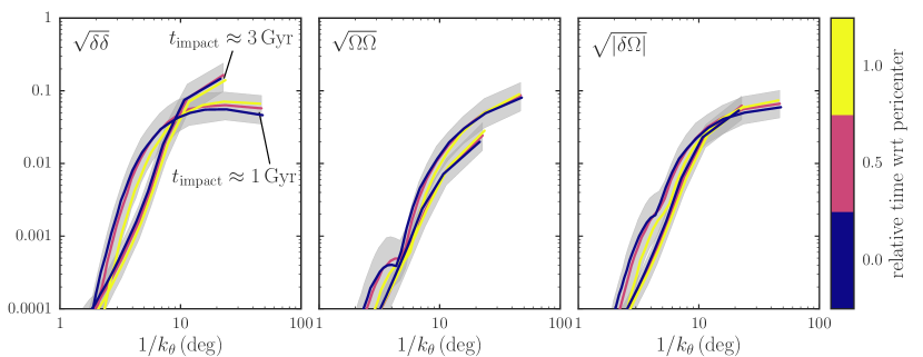
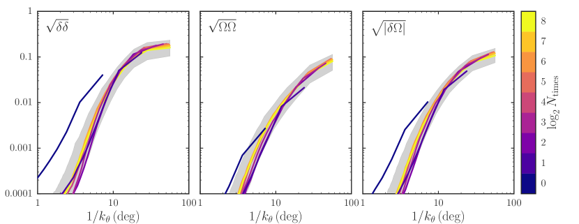
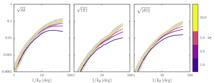
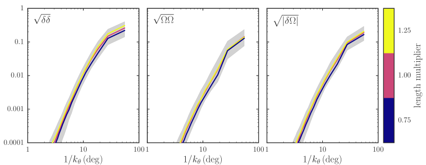
In this Appendix, we briefly discuss the results from a set of tests to assess whether the power spectra computed using our default sampling of subhalo impacts have converged. We test the three most important approximations in our statistical sampling of the impacts. These are (a) the resolution of the discrete time sampling, (b) the maximum possible impact parameter, and (c) the maximum distance along the stream to consider impacts at each impact time. While these convergence tests should be repeated for any new stream modeled using our framework, we derive some rules that should hold more generally than the specific simulation here.

We sample impacts on a discrete grid of times between the start of tidal disruption of the stellar stream and the present time. This saves computational time in the line-of-parallel-angle approach, because multiple impacts at the same time do not add to the computational cost. Our default simulation setup for the GD-1-like stream considers impacts at 64 different times or at a spacing of $\approx 140\,\mathrm{Myr}$. This is about one-third of the radial period of the approximate stream orbit, which is $400\,\mathrm{Myr}$. Sampling impact times on a finer grid essentially increases the coverage of the orbital phase of the stream at the impacts.

To assess the importance of sampling the orbital phase, we run simulations with a single value of the mass, here $10^{6.5}\,\mathrm{M}_{\odot}$, using the rate of impacts corresponding to masses between $10^{6}\,\mathrm{M}_{\odot}$ and $10^{7}\,\mathrm{M}_{\odot}$. Rather than sampling the entire range of times between the start of disruption and the current time, we apply all impacts at the same time. This time is chosen to be when the stream is near pericenter, apocenter, and halfway in between. We do this for two sets of such times, one $\approx 1\,\mathrm{Gyr}$ in the past and one $\approx 3\,\mathrm{Gyr}$ ago. The resulting power spectra are displayed in Figure 38. It is clear that the overall time at which the impact occurs is important: The impacts that happen $\approx 1\,\mathrm{Gyr}$ ago give rise to less power on large scales than those that happen $\approx 3\,\mathrm{Gyr},$ because they have not had enough time to evolve yet. However, the orbital phase at which the impact happens is much less important: all different phases near the same time give rise to the same power spectrum. Thus, the time sampling only needs to be fine enough to sample the overall history of the stream, but is not required to be so fine as to densely sample the orbital phase of each radial oscillation.

In Figure 39 we display the power spectrum computed using different-sized grids of equally-spaced times. We consider grids between that consisting of a single time at the mid-point between the start of disruption and the current time up to a grid with 256 different times (spacing $\approx 35\,\mathrm{Myr}$). This figure demonstrates that the power spectrum quickly converges, in agreement with the discussion in the preceding paragraph. The power spectrum has largely converged when using $16$ different times, which corresponds to a spacing of $\approx 560\,\mathrm{Myr}$, which is slightly larger than the radial period. The same convergence happens for other mass ranges ($10^{5}\,\mathrm{M}_{\odot}$–$10^{7}\,\mathrm{M}_{\odot}$ and $10^{7}\,\mathrm{M}_{\odot}$–$10^{8}\,\mathrm{M}_{\odot}$; see Figure 12). In general, we expect from the behavior in Figures 38 and 39 that sampling impact times somewhat finer than the radial period should always suffice to obtain a converged power spectrum.

The second simulation parameter that we consider in this Appendix is the maximum impact parameter. In $\mathsection$ 2.3, we describe how we sample impacts up to a maximum impact parameter that is a function of the mass of the perturber. We sample impact parameters up to a multiple $X$ of the scale radius of the perturbing subhalo. Equation (1) shows that the rate of impacts is linearly dependent on the maximum impact parameter and therefore also on $X$. Ideally, we would consider impacts out to an impact parameter of infinity, but this is not advisable both from a practical and a modeling perspective: Distant encounters are not well described by the impulse approximation that we use to compute the instantaneous effect of subhalo impacts. Practically, increasing the rate of encounters increases the computational cost significantly. Because we expect distant encounters to be subdominant (velocity kicks go as $M/b$ at large $b$), we therefore do not want to include unnecessary distant encounters.

In Figure 40 we display the $X$ dependence of the power spectrum for impacts with a single mass of $10^{5.5}\,\mathrm{M}_{\odot}$ using the rate corresponding to the range $10^{5}\,\mathrm{M}_{\odot}$ to $10^{6}\,\mathrm{M}_{\odot}$. While the power spectrum on small scales quickly converges once $X\approx 3$, the power on large scales keeps increasing as $X$ is increased. The same behavior occurs for other mass ranges (see Figure 12). To limit the computational cost, we use $X=5$ in our default setup, but it is clear from Figure 40 and Figure 12 that this underestimates the power on the largest scales. At these large distances, the impulse approximation will begin to break down so it is unclear whether this lack of convergence on large scales is as severe as it seems from Figure 40. If one is interested in using density and track fluctuations on the largest scales—which is only be possible for the longest streams with lengths $\gtrsim 30^{\circ}$—distant encounters are important and need to be taken into account. However, to compute the statistical properties of a tidal stream on the smallest scales, $X$ can safely be set to a value of a few.

Finally, in Figure 41 we vary the distance along the stream where we consider impacts. In our default setup, at each impact time we only consider impacts that happen closer to the progenitor than the length of the stream, defined at the end of $\mathsection$ 2.1. However, a tidal stream does not have a sharp end and impacts that occur beyond this nominal length could push stream stars back toward the progenitor where they could affect the current structure of the stream. Figure 41 demonstrates that at least for the GD-1-like stream this definition of the length is appropriate: the power spectrum is essentially the same when only considering impacts up to $75\,\%$ of the nominal length at each time and when considering impacts out to $125\,\%$ of the nominal length. Figure 41 shows this for impacts with a mass of $10^{7.5}\,\mathrm{M}_{\odot}$ using the rate for the mass range $10^{7}\,\mathrm{M}_{\odot}$ to $10^{8}\,\mathrm{M}_{\odot}$, but we find the same for lower mass ranges (see Figure 12). We expect our definition of the length to work well for most streams, at least for the small expected CDM-like impact rates.

Appendix D Mock Pal 5 rate analysis

Figure 42: Posterior probability distribution functions for the rate of dark–matter subhalo encounters based on mock simulations of the Pal 5 stream in a dark–matter halo with varying levels of substructure with masses between $10^{6}\,\mathrm{M}_{\odot}$ and $10^{9}\,\mathrm{M}_{\odot}$. The PDFs are obtained in the same manner as those for the real Pal 5 data in Figure 31. Different curves are the PDF for different levels of substructure: The orange line is for a simulation without any CDM halos, the purple curve for a simulation with a CDM-like population of subhalos (without accounting for any subhalo destruction by the disk), and the blue curve for a simulation with three times the CDM population. The vertical lines indicate the truth for each simulation. The downturn of the orange curve near $-1$ is an artifact due to the KDE method used to smooth the PDF, in reality it peaks at $-1$. All PDFs are consistent with the input rate within the width of the PDF, demonstrating that matching the observed power using simulations produced with our formalism can robustly constrain the amount of substructure in the halo.

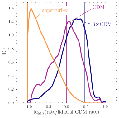
In this Appendix, we repeat the analysis of the Pal 5 data in $\mathsection$ 7 for a suite of mock-data simulations to test our procedure. These simulations were run with the $N$-body part of gadget-3 which is similar to gadget-2 (Springel, 2005). The code was modified to include external static potentials as well as the forces from the subhalos which were modeled as Hernquist profiles. These Hernquist profiles have the same size-mass relation given in $\mathsection$ 2.3. The best-fit phase–space position from Küpper et al. (2015) is integrated backward for $5\,\mathrm{Gyr}$. At this point, a King cluster with a mass of $2\times 10^{4}\,\mathrm{M}_{\odot}$, central-potential parameter $W_{0}=2$, and $r_{c}=15$ pc is instantiated with $100,000$ particles. This cluster is then integrated forward in time for $5\,\mathrm{Gyr}$ until the present day, using a softening of 1 pc. The smooth potential is similar to the MWPotential2014 used in the analysis of the real Pal 5 data, except that the bulge component has been replaced by a Hernquist sphere with the same mass and a scale radius of $500\,\mathrm{pc}$ (MWPotential2014 has a power-law bulge with an exponential cut-off that is computationally more complex). A population of subhalos is orbiting within this potential with a number density given by the Einasto fit in (Springel et al., 2008) scaled down to a mass of $10^{12}\,\mathrm{M}_{\odot}$. The full gravitational interaction between each subhalo and the stream is computed whenever the subhalo is within $30\,\mathrm{kpc}$ from the galactic center. We perform simulation (a) without any substructure, (b) with a CDM-like population of subhalos, and (c) with three times a CDM-like number of subhalos. At the end of the simulation, these end up at approximately the current position of Pal 5 and we analyze them in the same $(\xi,\eta)$ coordinate system as for the real data (we shift the simulations such that the surviving progenitor is located at $(\xi,\eta)=(0,0)$). We have also performed a simulation with ten times the amount of substructure expected for CDM. This produces a stream that is very far from the current position of Pal 5 and that is very significantly perturbed. It does not look like the observed Pal 5 stream, confirming that a rate as high as ten times CDM is obviously at odds with the observed Pal 5 stream. We do not consider this mock simulation further. The expected number of subhalos within $25\,\mathrm{kpc}$ for CDM for these simulations is slightly different than what we have used in the main body of this paper. The CDM-like number of subhalos within $25\,\mathrm{kpc}$ with masses between $10^{5}\,\mathrm{M}_{\odot}$ and $10^{9}\,\mathrm{M}_{\odot}$ in these mock simulations is $525.40$, obtained by rescaling the fits from the Aquarius simulation (Springel et al., 2008) (see Erkal et al. 2016 for further details).

We analyze the density data in of these three mock-Pal 5 streams in the same manner as the real Pal 5 data. That is, we compute the density in $0.1^{\circ}$ bins in $\xi$, normalize it using a third-order polynomial fit, calculate the power spectrum of the part of the stream between $0.2^{\circ}<\xi<14.3^{\circ}$, and match the power on the three largest scales and the bispectrum, using largely the same tolerances as for the real data. For the simulation without any substructure we change the tolerance for the power on the second- and third-largest scales to $0.01$, because the power in the mock data on these scales is very small, thus allowing us to make the tolerance smaller. For the CDM and $3\times$CDM simulations we relax the tolerance on the bispectrum slightly. As the uncertainties, we simply use the Poisson uncertainties on the number of $N$-body particles in each $\xi$ bin; the stream density is $\approx 500\,\mathrm{deg}^{-1}$ for all mock streams. The density uncertainties in the simulations are therefore typically $\approx 14\,\%$.

The resulting PDFs for the rate of impacts are displayed in Figure 42. It is clear that we can put a tight constraint on the incidence of substructure if there is no substructure (yellow curve). The $95\,\%$ and $99\,\%$ upper limits on the rate are $0.6\times$CDM and $1.0\times$CDM, respectively, just from the power on the three largest scales and the bispectrum on a single scale. We could have used the power on smaller scales to get a better constraint, but we are here primarily interested in testing the robustness of our Pal 5 analysis, for which this is not possible. For the mock data perturbed by a CDM-like or $3\times$CDM-like population of subhalos, we find relatively broad PDFs similar to the PDF for the real Pal 5 data in Figure 31. These are both consistent with the input value for the rate, which in both cases lies about $1\sigma$ from the peak of the PDF. The reason that the PDFs are not narrower than those for the Pal 5 data in $\mathsection$ 7 even though the mock-data uncertainties are four times smaller than those for the Pal 5 data is that the power on the largest scales is much larger than the noise power. The measurement of this large-scale power is therefore limited by the fact that we only have a single realization of the density to measure the power and not by the uncertainties in the density measurement: the uncertainty in the power is the power itself (Press et al., 2007).

In addition to the results displayed in Figure 31, we have performed three more simulations each of perturbations from a CDM-like and $3\times$CDM-like population. The resulting PDFs are similar to those shown here and we find no significant biases in the inferred rate. Thus, we conclude that our procedure of matching the power on the largest scales to constrain the number of subhalos with the Pal 5 data is robust.

References

- Amorisco (2015) Amorisco N. C., 2015, MNRAS, 450, 575
- Binney & McMillan (2016) Binney J., McMillan P. J., 2016, MNRAS, 456, 1982
- Bonaca et al. (2014) Bonaca A., Geha M., Kuepper A. H. W., Diemand J., Johnston K. V., Hogg D. W., 2014, ApJ, 795, 94
- Bovy (2014) Bovy J., 2014, ApJ, 795, 95
- Bovy (2015) Bovy J., 2015, ApJS, 216, 29
- Bovy (2016) Bovy J., 2016, PRL, 116, 121301
- Bovy & Rix (2013) Bovy J., Rix H.-W., 2013, ApJ, 779, 115
- Bowden et al. (2015) Bowden A., Belokurov V., Evans N. W., 2015, MNRAS, 449, 1391
- Carlberg (2009) Carlberg R. G., 2009, ApJL, 705, L223
- Carlberg (2012) Carlberg R. G., 2012, ApJ, 748, 20
- Carlberg (2013) Carlberg R. G., 2013, ApJ, 775, 90
- Carlberg (2016) Carlberg R. G., 2016, ApJ, 820, 45
- Carlberg & Grillmair (2013) Carlberg R. G., Grillmair C. J., 2013, ApJ, 768, 171
- Carlberg et al. (2012) Carlberg R. G., Grillmair C. J., Hetherington N., 2012, ApJ, 760, 75
- Chiba (2002) Chiba M., 2002, ApJ, 565, 17
- Dalal & Kochanek (2002) Dalal N., Kochanek C. S., 2002, ApJ, 572, 25
- Dehnen et al. (2004) Dehnen W., Odenkirchen M., Grebel E. K., Rix H.-W., 2004, AJ, 127, 2753
- Diemand et al. (2007) Diemand J., Kuhlen M., Madau P., 2007, ApJ, 667, 859
- Diemand et al. (2008) Diemand J., Kuhlen M., Madau P., Zemp M., Moore B., Potter D., Stadel J., 2008, Nature, 454, 735
- Diemand et al. (2004) Diemand J., Moore B., Stadel J., 2004, MNRAS, 352, 535
- D’Onghia et al. (2010) D’Onghia E., Springel V., Hernquist L., Keres D., 2010, ApJ, 709, 1138
- Elgar (1987) Elgar S., 1987, IEEE Trans. Acoustics, Speech, and Signal Processing, 35, 1725
- Erkal & Belokurov (2015a) Erkal D., Belokurov V., 2015a, MNRAS, 450, 1136
- Erkal & Belokurov (2015b) Erkal D., Belokurov V., 2015b, MNRAS, 454, 3542
- Erkal et al. (2016) Erkal D., Belokurov V., Bovy J., Sanders J. L., 2016, MNRAS, 463, 102
- Eyre & Binney (2011) Eyre A., Binney J., 2011, MNRAS, 413, 1852
- Fardal et al. (2015) Fardal M. A., Huang S., Weinberg M. D., 2015, MNRAS, 452, 301
- Fritz & Kallivayalil (2015) Fritz T. K., Kallivayalil N., 2015, ApJ, 811, 123
- Gibbons et al. (2014) Gibbons S. L. J., Belokurov V., Evans N. W., 2014, MNRAS, 445, 3788
- Grillmair (2009) Grillmair C. J., 2009, ApJ, 693, 1118
- Grillmair & Dionatos (2006) Grillmair C. J., Dionatos O., 2006, ApJ, 643, L17
- Helmi & White (1999) Helmi A., White S. D. M., 1999, MNRAS, 307, 495
- Hezaveh et al. (2016) Hezaveh Y. D. et al., 2016, arXiv:1601.01388
- Hofmann et al. (2001) Hofmann S., Schwarz D. J., Stöcker H., 2001, PRD, 64, 083507
- Ibata et al. (2002) Ibata R. A., Lewis G. F., Irwin M. J., Quinn T., 2002, MNRAS, 332, 915
- Ibata et al. (2016) Ibata R. A., Lewis G. F., Martin N. F., 2016, ApJ, 819, 1
- Johnston (1998) Johnston K. V., 1998, ApJ, 495, 297
- Johnston et al. (2002) Johnston K. V., Spergel D. N., Haydn C., 2002, ApJ, 570, 656
- Jones et al. (2001) Jones E., Oliphant T., Peterson P., et al., 2001, SciPy: Open source scientific tools for Python
- Klypin et al. (1999) Klypin A., Kravtsov A. V., Valenzuela O., Prada F., 1999, ApJ, 522, 82
- Koposov et al. (2010) Koposov S. E., Rix H.-W., Hogg D. W., 2010, ApJ, 712, 260
- Koposov et al. (2009) Koposov S. E., Yoo J., Rix H.-W., Weinberg D. H., Macciò A. V., Escudé J. M., 2009, ApJ, 696, 2179
- Küpper et al. (2015) Küpper A. H. W., Balbinot E., Bonaca A., Johnston K. V., Hogg D. W., Kroupa P., Santiago B. X., 2015, ApJ, 803, 80
- Küpper et al. (2010) Küpper A. H. W., Kroupa P., Baumgardt H., Heggie D. C., 2010, MNRAS, 401, 105
- Küpper et al. (2012) Küpper A. H. W., Lane R. R., Heggie D. C., 2012, MNRAS, 420, 2700
- Kuzma et al. (2015) Kuzma P. B., Da Costa G. S., Keller S. C., Maunder E., 2015, MNRAS, 446, 3297
- Lacey & Ostriker (1985) Lacey C. G., Ostriker J. P., 1985, ApJ, 299, 633
- Mao & Schneider (1998) Mao S., Schneider P., 1998, MNRAS, 295, 587
- Marin et al. (2012) Marin J. M., Pudlo P., Robert C. P., Ryder R. J., 2012, Stat. Comput., 22, 1167
- Masuda & Kuo (1981) Masuda A., Kuo Y., 1981, Deep-Sea Res., 28A, 213
- Moore et al. (1999) Moore B., Ghigna S., Governato F., Lake G., Quinn T., Stadel J., Tozzi P., 1999, ApJL, 524, L19
- Ngan et al. (2016) Ngan W., Carlberg R. G., Bozek B., Wyse R. F. G., Szalay A. S., Madau P., 2016, ApJ, 818, 194
- Ngan & Carlberg (2014) Ngan W. H. W., Carlberg R. G., 2014, ApJ, 788, 181
- Odenkirchen et al. (2003) Odenkirchen M. et al., 2003, AJ, 126, 2385
- Odenkirchen et al. (2001) Odenkirchen M., et al., 2001, ApJ, 548, L165
- Piffl et al. (2015) Piffl T., Penoyre Z., Binney J., 2015, MNRAS, 451, 639
- Press et al. (2007) Press W. H., Teukolsky S. A., Vetterling W. T., Flannery B. P., 2007, Numerical Recipes 3rd Edition: The Art of Scientific Computing, 3rd edn. Cambridge University Press, New York, NY, USA
- Price-Whelan et al. (2014) Price-Whelan A. M., Hogg D. W., Johnston K. V., Hendel D., 2014, ApJ, 794, 4
- Profumo et al. (2006) Profumo S., Sigurdson K., Kamionkowski M., 2006, PRL, 97
- Rao & Gabr (1984) Rao T., Gabr M., 1984, An introduction to bispectral analysis and bilinear time series models, Lecture notes in statistics. Springer-Verlag
- Rosolowsky (2005) Rosolowsky E., 2005, PASP, 117, 1403
- Sanders (2014) Sanders J. L., 2014, MNRAS, 443, 423
- Sanders & Binney (2013) Sanders J. L., Binney J., 2013, MNRAS, 433, 1813
- Sanders & Binney (2014) Sanders J. L., Binney J., 2014, MNRAS, 441, 3284
- Sanders et al. (2016) Sanders J. L., Bovy J., Erkal D., 2016, MNRAS, 457, 3817
- Schmid et al. (1999) Schmid C., Schwarz D. J., Widerin P., 1999, PRD, 59
- Siegal-Gaskins & Valluri (2008) Siegal-Gaskins J. M., Valluri M., 2008, ApJ, 681, 40
- Sirko et al. (2004) Sirko E. et al., 2004, AJ, 127, 914
- Springel (2005) Springel V., 2005, MNRAS, 364, 1105
- Springel et al. (2008) Springel V. et al., 2008, MNRAS, 391, 1685
- Strigari et al. (2008) Strigari L. E., Bullock J. S., Kaplinghat M., Simon J. D., Geha M., Willman B., Walker M. G., 2008, Nature, 454, 1096
- Tremaine (1999) Tremaine S., 1999, MNRAS, 307, 877
- Varghese et al. (2011) Varghese A., Ibata R., Lewis G. F., 2011, MNRAS, 417, 198
- Vegetti et al. (2012) Vegetti S., Lagattuta D. J., McKean J. P., Auger M. W., Fassnacht C. D., Koopmans L. V. E., 2012, Nature, 481, 341
- Viel et al. (2013) Viel M., Becker G. D., Bolton J. S., Haehnelt M. G., 2013, PRD, 88, 043502
- Viel et al. (2005) Viel M., Lesgourgues J., Haehnelt M. G., Matarrese S., Riotto A., 2005, PRD, 71, 063534
- Yoon et al. (2011) Yoon J. H., Johnston K. V., Hogg D. W., 2011, ApJ, 731, 58