CERN-PH-TH-2016-138, CP3-16-29, NSF-KITP-16-084

Jet production in the CoLoRFulNNLO method:

event shapes in electron-positron collisions

Vittorio Del Duca^(a), Claude Duhr^(b,c), Adam Kardos^(d,e), Gábor Somogyi^(d),

Zoltán Szőr^(d,e), Zoltán Trócsányi^(d,e)  and  Zoltán Tulipánt^(d)

^(a) Institute for Theoretical Physics, ETH Zürich, 8093 Zürich, Switzerland

^(b) Theoretical Physics Department, CERN, CH-1211 Geneva 23, Switzerland

^(c) Center for Cosmology, Particle Physics and Phenomenology (CP3), Université Catholique de Louvain, Chemin du Cyclotron 2, B-1348 Louvain-La-Neuve, Belgium

^(d) University of Debrecen and MTA-DE Particle Physics Research Group H-4010 Debrecen, PO Box 105, Hungary

^(e) Kavli Institute for Theoretical Physics, University of California, Santa Barbara, CA 93106, USA

Abstract

We present the CoLoRFulNNLO method to compute higher order radiative corrections to jet cross sections in perturbative QCD. We apply our method to the computation of event shape observables in electron-positron collisions at NNLO accuracy and validate our code by comparing our predictions to previous results in the literature. We also calculate for the first time jet cone energy fraction at NNLO.

June 2016

1 Introduction

The strong coupling $\alpha_{\rm{s}}$ is one of the most important parameters of the standard model. A clean environment for determining $\alpha_{\rm{s}}$ is the study of event shape distributions in electron-positron collisions. Particularly well suited for this task are quantities related to three-jet events, as the leading term in a perturbative description of such observables is already proportional to the strong coupling. Accordingly, three-jet event shapes were measured extensively, especially at LEP [1, 2, 3, 4]. The precision of experimental measurements calls for an equally precise theoretical description of these quantities. Because the strong interactions occur only in the final state, non-perturbative QCD corrections are restricted to hadronization and power corrections. These corrections can be determined either by extracting them from data by comparison to Monte Carlo predictions or by using analytic models. Hence, the precision of the theoretical predictions is mostly limited by the truncation of the perturbative expansion in the strong coupling.

Current state-of-the art includes next-to-next-to-leading order (NNLO) predictions for the three-jet event shapes of thrust, heavy jet mass, total and wide jet broadening, $C$-parameter and the two-to-three jet transition variable $y_{23}$ [5, 6], as well as for oblateness and energy-energy correlation [7]. Next-to-leading order (NLO) predictions for the production of up to five jets [8, 9, 10, 11, 12] (and up to seven jets in the leading color approximation [13]) are also known. Moreover, logarithmically enhanced contributions to event shapes can be resummed at up to next-to-next-to-leading logarithmic (NNLL) accuracy [14, 15, 16, 17, 18] and even at next-to-next-to-next-to-leading logarithmic ($\rm N^{3}LL$) accuracy for some observables [19, 20].

In addition to its phenomenological relevance, three-jet production in electron-positron collisions is also an ideal testing ground for developing general tools and techniques for higher-order calculations in QCD. The straightforward evaluation of radiative corrections in QCD is hampered by the presence of infrared singularities in intermediate stages of the calculation which cancel in the final physical results for these observables. Nevertheless, they must be regularized and their cancellation has to be made explicit before any numerical computation can be performed. This turns out to be rather involved for fully differential cross sections at NNLO and constructing a method to regularize infrared divergences has been an ongoing task for many years [21, 22, 23, 24, 25, 26, 27, 28, 29, 30, 31, 32, 33, 34, 35, 36, 37, 38, 39, 40, 41, 42, 43, 44, 45, 46, 47, 48, 49, 50, 51, 52, 53].

In this paper we present a general subtraction scheme to compute fully differential predictions at NNLO accuracy, called CoLoRFulNNLO (Completely Local subtRactions for Fully differential predictions at NNLO accuracy) [41, 42, 43, 44, 45, 46, 47, 48, 49, 50, 51]. The method uses the known universal factorization properties of QCD matrix elements in soft and collinear limits [54, 55, 56, 57, 58, 59, 60, 61, 62] to construct completely local subtraction terms which regularize infrared singularities associated with unresolved real emission. Virtual contributions are rendered finite by adding back the subtractions after integration and summation over the phase space and quantum numbers (color and flavor) of the unresolved emission. We have worked out the method completely for processes with a colorless initial state and involving any number of colored massless particles in the final state. We validate our method and code by computing NNLO corrections to three-jet event shape variables and comparing our predictions to those available in the literature [5, 6]. We also present here for the first time the computation of the jet cone energy fraction (JCEF) at NNLO accuracy. We note that the CoLoRFulNNLO method has already been successfully applied to compute NNLO corrections to differential distributions describing the decay of a Higgs boson into a pair of b-quarks [63], as well as to the computation of oblateness and energy-energy correlation in $e^{+}e^{-}\to 3$ jet production [7].

The paper is structured as follows: after introducing our notation and conventions in section 2, we present the CoLoRFulNNLO method in section 3. In section 4 we describe the application of the general framework to the specific case of three-jet production. In particular, we show that the double virtual contribution is free of singularities. Our predictions for event shape observables follow in section 5. We draw our conclusions and give our outlook in section 6.

2 Notation and conventions

2.1 Phase space and kinematics

The phase space measure in $d=4-2\epsilon$ dimensions for a total incoming momentum $Q^{\mu}$ and $n$ massless outgoing particles reads

$${\rm{d}}\phi_{n}(Q^{2})\equiv{\rm{d}}\phi_{n}\big{(}p_{1}^{\mu},\ldots,p_{n}^{\mu};Q^{\mu}\big{)}=\Bigg{[}\prod_{i=1}^{n}\frac{{\rm{d}}^{d}p_{i}}{(2\pi)^{d-1}}\delta_{+}(p_{i}^{2})\Bigg{]}(2\pi)^{d}\delta^{(d)}\big{(}p_{1}^{\mu}+\ldots+p_{n}^{\mu}-Q^{\mu}\big{)}\,.$$ (2.1)

Throughout the paper, we will use $y_{ik}$ to denote twice the dot-product of two momenta, scaled by the total momentum squared $Q^{2}$. For example,

$$y_{ik}=\frac{2p_{i}\cdot p_{k}}{Q^{2}}=\frac{s_{ik}}{Q^{2}}\qquad\mbox{and}\qquad y_{iQ}=\frac{2p_{i}\cdot Q}{Q^{2}}\,.$$ (2.2)

We also introduce the combination

$$Y_{ik,Q}=\frac{y_{ik}}{y_{iQ}y_{kQ}}$$ (2.3)

for later convenience.

2.2 Matrix elements

We use the color and spin space notation of ref. [64] where the renormalized matrix element for a given process with $n$ particles in the final state, $|{\cal M}_{n}\rangle$, is a vector in color and spin space, normalized such that the squared matrix element summed over colors and spins is given by

$$|{\cal M}_{n}{}|^{2}=\langle{\cal M}_{n}|{\cal M}_{n}\rangle\,.$$ (2.4)

The renormalized matrix element has the following formal loop expansion

$$|{\cal M}_{n}\rangle=|{\cal M}_{n}^{(0)}\rangle+|{\cal M}_{n}^{(1)}\rangle+|{\cal M}_{n}^{(2)}\rangle+\ldots\,,$$ (2.5)

where the superscript denotes the number of loops. We will always consider matrix elements computed in conventional dimensional regularization (CDR) with $\overline{\rm{MS}}$ subtraction. We introduce the following notation to indicate color-correlated squared matrix elements (obtained by the insertion of color charge operators between $\langle{\cal M}_{n}^{(\ell_{1})}|$ and $|{\cal M}_{n}^{(\ell_{2})}\rangle$):

$$\begin{split}\langle{\cal M}^{(\ell_{1})}|{\cal M}^{(\ell_{2})}\rangle\otimes{\mbox{\boldmath$T$}}_{i}\!\cdot\!{\mbox{\boldmath$T$}}_{k}&=\langle{\cal M}^{(\ell_{1})}|\,{\mbox{\boldmath$T$}}_{i}\!\cdot\!{\mbox{\boldmath$T$}}_{k}\,|{\cal M}_{n}^{(\ell_{2})}\rangle\,,\\[5.69054pt] \langle{\cal M}^{(\ell_{1})}|{\cal M}^{(\ell_{2})}\rangle\otimes\{{\mbox{\boldmath$T$}}_{i}\!\cdot\!{\mbox{\boldmath$T$}}_{k},{\mbox{\boldmath$T$}}_{j}\!\cdot\!{\mbox{\boldmath$T$}}_{l}\}&=\langle{\cal M}^{(\ell_{1})}|\{{\mbox{\boldmath$T$}}_{i}\!\cdot\!{\mbox{\boldmath$T$}}_{k},{\mbox{\boldmath$T$}}_{j}\!\cdot\!{\mbox{\boldmath$T$}}_{l}\}|{\cal M}^{(\ell_{2})}\rangle\,.\end{split}$$ (2.6)

The color charge algebra for the product $\sum_{a}({\mbox{\boldmath$T$}}_{i})^{a}({\mbox{\boldmath$T$}}_{k})^{a}\equiv{\mbox{\boldmath$T$}}_{i}\!\cdot\!{\mbox{\boldmath$T$}}_{k}$ is

$${\mbox{\boldmath$T$}}_{i}\!\cdot\!{\mbox{\boldmath$T$}}_{k}={\mbox{\boldmath$T$}}_{k}\!\cdot\!{\mbox{\boldmath$T$}}_{i}\,,\quad\mbox{if}\quad i\neq k\qquad\mbox{and}\qquad{\mbox{\boldmath$T$}}_{i}^{2}=C_{i}\,,$$ (2.7)

where $C_{i}$ is the quadratic Casimir operator in the representation of particle $i$. We use the customary normalization $T_{\rm{R}}=1/2$, and so $C_{\rm{A}}=2T_{\rm{R}}N_{\rm{c}}=N_{\rm{c}}$ in the adjoint and $C_{\rm{F}}=T_{\rm{R}}(N_{\rm{c}}^{2}-1)/N_{\rm{c}}=(N_{\rm{c}}^{2}-1)/(2N_{\rm{c}})$ in the fundamental representation.

2.3 Ultraviolet renormalization

In massless QCD renormalized amplitudes $|{\cal M}_{n}\rangle$ are obtained from the corresponding unrenormalized amplitudes $|{\cal A}_{n}\rangle$ by replacing the bare coupling $\alpha_{\rm{s}}^{B}$ with the dimensionless renormalized coupling $\alpha_{\rm{s}}\equiv\alpha_{\rm{s}}(\mu)$ computed in the $\overline{\rm{MS}}$ scheme and evaluated at the renormalization scale $\mu$,

$$\alpha_{\rm{s}}^{B}\mu_{0}^{2\epsilon}\,S_{\epsilon}^{\overline{\rm{MS}}}=\alpha_{\rm{s}}\mu^{2\epsilon}\bigg{[}1-\frac{\alpha_{\rm{s}}}{4\pi}\frac{\beta_{0}}{\epsilon}+\left(\frac{\alpha_{\rm{s}}}{4\pi}\right)^{2}\left(\frac{\beta_{0}^{2}}{\epsilon^{2}}-\frac{\beta_{1}}{2\epsilon}\right)+\rm O(\alpha_{\rm{s}}^{3})\bigg{]}\,,$$ (2.8)

where

$$\beta_{0}=\frac{11C_{\rm{A}}}{3}-\frac{4n_{\rm{f}}T_{\rm{R}}}{3}\,,\quad\beta_{1}=\frac{34}{3}C_{\rm{A}}^{2}-\frac{20}{3}C_{\rm{A}}T_{\rm{R}}n_{\rm{f}}-4C_{\rm{F}}T_{\rm{R}}n_{\rm{f}}\,,$$ (2.9)

and $S_{\epsilon}^{\overline{\rm{MS}}}=(4\pi)^{\epsilon}\exp(-\epsilon\gamma_{\rm{E}})$ corresponds to $\overline{\rm{MS}}$ subtraction, with $\gamma_{\rm{E}}=-\Gamma^{\prime}(1)$ the Euler–Mascheroni constant. Although the factor $(4\pi)^{\epsilon}\exp(-\epsilon\gamma_{\rm{E}})$ is often abbreviated as $S_{\epsilon}$ in the literature, we reserve the latter to denote

$$S_{\epsilon}=\frac{(4\pi)^{\epsilon}}{\Gamma(1-\epsilon)}\,,$$ (2.10)

which emerges in the integration of the angular part of the phase space in $d=4-2\epsilon$ dimensions. If the loop expansion of the unrenormalized amplitude is written as

$$|{\cal A}_{m}\rangle=(4\pi\alpha_{\rm{s}}^{B})^{\frac{q}{2}}\bigg{[}|{\cal A}_{m}^{(0)}\rangle+\frac{\alpha_{\rm{s}}^{B}}{4\pi}\,|{\cal A}_{m}^{(1)}\rangle+\left(\frac{\alpha_{\rm{s}}^{B}}{4\pi}\right)^{2}|{\cal A}_{m}^{(2)}\rangle+\rm O(\alpha_{\rm{s}}^{3})\bigg{]}\,,$$ (2.11)

(with $q=m-2$, where $m$ is the number of massless final-state partons in the Born process) then using the substitution in eq. (2.8) the relations between the renormalized and the unrenormalized amplitudes are given as follows:

$$|{\cal M}_{m}^{(0)}\rangle=C(\mu,\mu_{0},q;\epsilon)|{\cal A}_{m}^{(0)}\rangle\,,$$ (2.12)

$$|{\cal M}_{m}^{(1)}\rangle=C(\mu,\mu_{0},q;\epsilon)\frac{\alpha_{\rm{s}}}{4\pi}\left[\left(\frac{\mu^{2}}{\mu_{0}^{2}}\right)^{\epsilon}\left(S_{\epsilon}^{\overline{\rm{MS}}}\right)^{-1}|{\cal A}_{m}^{(1)}\rangle-\frac{q}{2}\frac{\beta_{0}}{\epsilon}\,|{\cal A}_{m}^{(0)}\rangle\right]$$ (2.13)

and

$$\begin{split}|{\cal M}_{m}^{(2)}\rangle=C(\mu,\mu_{0},q;\epsilon)\left(\frac{\alpha_{\rm{s}}}{4\pi}\right)^{2}&\Bigg{[}\left(\frac{\mu^{2}}{\mu_{0}^{2}}\right)^{2\epsilon}\left(S_{\epsilon}^{\overline{\rm{MS}}}\right)^{-2}|{\cal A}_{m}^{(2)}\rangle-\frac{q+2}{2}\frac{\beta_{0}}{\epsilon}\left(\frac{\mu^{2}}{\mu_{0}^{2}}\right)^{\epsilon}\left(S_{\epsilon}^{\overline{\rm{MS}}}\right)^{-1}|{\cal A}_{m}^{(1)}\rangle\\ &+\frac{q}{2}\left(\frac{q+2}{4}\frac{\beta_{0}^{2}}{\epsilon^{2}}-\frac{\beta_{1}}{\epsilon}\right)\,|{\cal A}_{m}^{(0)}\rangle\Bigg{]}\,,\end{split}$$ (2.14)

where

$$C(\mu,\mu_{0},q;\epsilon)=(4\pi\alpha_{\rm{s}})^{\frac{q}{2}}\left(\frac{\mu^{2}}{\mu_{0}^{2}}\right)^{\frac{q}{2}\epsilon}\left(S_{\epsilon}^{\overline{\rm{MS}}}\right)^{-\frac{q}{2}}\,.$$ (2.15)

The role of the factors of $(\mu^{2}/\mu_{0}^{2})^{\epsilon}$ is to change the regularization scale to the renormalization scale so that the renormalized amplitudes in eqs. (2.12)–(2.14) only depend on $\mu$. Furthermore, after the IR poles are canceled in a fixed order computation, we may set $\epsilon=0$, therefore, the factors of $(\mu^{2}/\mu_{0}^{2})^{\epsilon}$ and $S_{\epsilon}^{\overline{\rm{MS}}}$ in $C(\mu,\mu_{0},q;\epsilon)$ do not give any contribution, so we may perform the replacement

$$C(\mu,\mu_{0},q;\epsilon)\to(4\pi\alpha_{\rm{s}})^{\frac{q}{2}}\,.$$ (2.16)

3 Jet production in CoLoRFulNNLO

We consider the production of $m$ jets from a colorless initial state as in, e.g., Higgs boson decay or electron-positron annihilation into hadrons. In perturbative QCD the cross section for this process is given by an expansion in powers of the strong coupling $\alpha_{\rm{s}}$. At NNLO accuracy we retain the first three terms in this expansion

$$\sigma=\sigma^{\rm{LO}}+\sigma^{\rm{NLO}}+\sigma^{\rm{NNLO}}+\ldots\,.$$ (3.1)

The leading order contribution is simply given by the integral of the fully differential Born cross section ${\rm{d}}\sigma^{{\rm B}}_{m}$ of $m$ final-state partons over the the available $m$-parton phase space defined by the observable $J$, (often called jet function)

$$\sigma^{\rm{LO}}[J]=\int_{m}{\rm{d}}\sigma^{{\rm B}}_{m}J_{m}\,.$$ (3.2)

Here and in the following $J_{m}$ denotes the value of the infrared-safe observable $J$ evaluated on a final state with $m$ partons.

3.1 The NLO correction

The NLO correction is a sum of the real radiation and one-loop virtual terms,

$$\sigma^{\rm{NLO}}[J]=\int_{m+1}{\rm{d}}\sigma^{{\rm R}}_{m+1}J_{m+1}+\int_{m}{\rm{d}}\sigma^{{\rm V}}_{m}J_{m}\,,$$ (3.3)

both divergent in four dimensions. These two contributions can be made finite simultaneously by subtracting and adding back a suitably defined approximate cross section ${\rm{d}}\sigma^{{\rm R,A}_{\scriptscriptstyle 1}}_{m+1}$,

$$\sigma^{\rm{NLO}}[J]=\int_{m+1}\Big{[}{\rm{d}}\sigma^{{\rm R}}_{m+1}J_{m+1}-{\rm{d}}\sigma^{{\rm R,A}_{\scriptscriptstyle 1}}_{m+1}J_{m}\Big{]}_{d=4}+\int_{m}\Big{[}{\rm{d}}\sigma^{{\rm V}}_{m}+\int_{1}{\rm{d}}\sigma^{{\rm R,A}_{\scriptscriptstyle 1}}_{m+1}\Big{]}_{d=4}J_{m}\,.$$ (3.4)

Several prescriptions are available for the explicit construction of the approximate cross section [65, 64, 66, 42, 47]. Specifically in the CoLoRFulNNLO framework, it is written as

$${\rm{d}}\sigma^{{\rm R,A}_{\scriptscriptstyle 1}}_{m+1}=\frac{1}{2s}{\rm{d}}\phi_{m+1}(Q^{2}){\cal A}_{1}|{\cal M}_{m+1}^{(0)}{}|^{2}\,,$$ (3.5)

where the approximate matrix element for processes with $m+1$ partons in the final state is given by [42, 43],

$${\cal A}_{1}|{\cal M}_{m+1}^{(0)}{}|^{2}=\sum_{r=1}^{m+1}\Bigg{[}\sum_{\begin{subarray}{c}i=1\\ i\neq r\end{subarray}}^{m+1}\frac{1}{2}{\cal C}_{ir}^{(0,0)}-\Bigg{(}{\cal S}_{r}^{(0,0)}-\sum_{\begin{subarray}{c}i=1\\ i\neq r\end{subarray}}^{m+1}{\cal C}_{ir}{\cal S}_{r}^{(0,0)}\Bigg{)}\Bigg{]}\,.$$ (3.6)

On the right-hand side of eq. (3.6), ${\cal C}_{ir}^{(0,0)}$ and ${\cal S}_{r}^{(0,0)}$ denote counterterms which regularize the ${\vec{p}}_{i}||{\vec{p}}_{r}$ collinear limit and the $p_{r}^{\mu}\to 0$ soft limit in arbitrary dimensions. The role of the ${\cal C}_{ir}{\cal S}_{r}^{(0,0)}$ soft-collinear counterterm is to make sure that no double subtraction takes place in the overlapping soft-collinear phase space region. These counterterms were all defined explicitly in refs. [42, 43]. In our convention the indices of ${\cal C}_{ir}^{(0,0)}$ are not ordered, ${\cal C}_{ir}^{(0,0)}={\cal C}_{ri}^{(0,0)}$. As the sums in eq. (3.6) over $i$ and $r$ are likewise not ordered, the factor of $\frac{1}{2}$ is needed so that we count each collinear limit precisely once. Finally, the meaning of the superscript $(\ell_{1},\ell_{2})$ is the following: The corresponding counterterm involves the product of an $\ell_{1}$-loop unresolved kernel (an Altarelli–Parisi splitting function or a soft eikonal current) with an $\ell_{2}$-loop squared matrix element (in color or spin space). Specifically, $(0,0)$ means that in these subtraction terms a tree level collinear or soft function acts on a tree level reduced matrix element. Such superscripts will appear also for other counterterms throughout the paper.

Importantly, the approximate matrix element in eq. (3.6) takes into account all color and spin correlations in infrared limits, and hence it is a completely local and fully differential regulator of the real emission matrix element over the $m+1$-particle phase space. The complete locality of the subtraction is a necessary condition for the regularized real contribution,

$$\sigma^{\rm{NLO}}_{m+1}[J]=\int_{m+1}\Big{[}{\rm{d}}\sigma^{{\rm R}}_{m+1}J_{m+1}-{\rm{d}}\sigma^{{\rm R,A}_{\scriptscriptstyle 1}}_{m+1}J_{m}\Big{]}_{d=4}\,,$$ (3.7)

to be well-defined in four dimensions. As pointed out long ago [64], when the subtraction terms are not fully local, for instance because spin correlations in gluon decay are neglected, the evaluation of the difference $\int_{m+1}\left[{\rm{d}}\sigma^{{\rm R}}_{m+1}J_{m+1}-{\rm{d}}\sigma^{{\rm R,A}_{\scriptscriptstyle 1}}_{m+1}J_{m}\right]_{d=4}$ usually involves double angular integrals of the type $\int_{-1}^{1}{\rm{d}}(\cos\theta)\int_{0}^{2\pi}{\rm{d}}\phi\,\cos\phi/(1-\cos\theta)$ where $\phi$ is the azimuthal angle. These integrals are ill-defined. If their numerical integration is attempted, one can obtain any answer whatsoever (including the correct one) depending on the details of the integration procedure. (The correct answer is obtained by performing the integral analytically before going to four dimensions: $\int_{-1}^{1}{\rm{d}}(\cos\theta)\,\sin^{-2\epsilon}\theta\int_{0}^{2\pi}{\rm{d}}\phi\,\,\sin^{-2\epsilon}\phi\cos\phi/(1-\cos\theta)=0$.) Thus non-local subtractions alone are not sufficient to define correctly $\sigma^{\rm{NLO}}_{m+1}[J]$. Rather, the definition must be supplemented by the precise specification of an integration procedure which must be shown to give the correct numerical values for all integrals that are finite away from $d=4$, but whose four-dimensional value is ill-defined. As in CoLoRFulNNLO the subtractions are completely local, eq. (3.7) is well-defined in four dimensions as it is and may be computed with whatever numerical procedure is most convenient. These remarks apply also to the regularized double real and real-virtual cross sections in eqs. (3.14) and (3.15) which enter the NNLO correction.

Turning to the virtual contribution, the Kinoshita–Lee–Nauenberg (KLN) theorem ensures that the integral of the approximate cross section precisely cancels the divergences of the virtual piece for infrared-safe observables, so adding back what we have subtracted from the real correction, the virtual contribution becomes finite as well. We have performed the integration of the various subtraction terms analytically in ref. [42] and here we only quote the result, which can be written as,

$$\int_{1}{\rm{d}}\sigma^{{\rm R,A}_{\scriptscriptstyle 1}}_{m+1}={\rm{d}}\sigma^{{\rm B}}_{m}\otimes{\mbox{\boldmath$I$}}_{1}^{(0)}(\{p\}_{m};\epsilon)\,,$$ (3.8)

where the $\otimes$ product is defined in eq. (2.6) and the insertion operator is in general given by [42]

$${\mbox{\boldmath$I$}}_{1}^{(0)}(\{p\}_{m};\epsilon)=\frac{\alpha_{\rm{s}}}{2\pi}\frac{S_{\epsilon}}{S_{\epsilon}^{\overline{\rm{MS}}}}\bigg{(}\frac{\mu^{2}}{Q^{2}}\bigg{)}^{\epsilon}\sum_{i=1}^{m}\bigg{[}{{\rm C}}_{1,i}^{(0)}(y_{iQ};\epsilon){\mbox{\boldmath$T$}}_{i}^{2}+\sum_{\begin{subarray}{c}k=1\\ k\neq i\end{subarray}}^{m}{{\rm S}}_{1}^{(0),(i,k)}(Y_{ik,Q};\epsilon){\mbox{\boldmath$T$}}_{i}\!\cdot\!{\mbox{\boldmath$T$}}_{k}\bigg{]}\,.$$ (3.9)

The variables $Q^{\mu}$, $y_{iQ}$ and $Y_{ik,Q}$ were defined in section 2.1. The kinematic functions ${{\rm C}}_{1,i}^{(0)}(y_{iQ};\epsilon)$ and ${{\rm S}}_{1}^{(0),(i,k)}(Y_{ik,Q};\epsilon)$ have been computed as Laurent expansions in $\epsilon$ in ref. [42]. They are needed up to finite terms in a computation at NLO accuracy and up to $\rm O(\epsilon^{2})$ in a computation at NNLO accuracy. We present these kinematic functions explicitly up to $\rm O(\epsilon)$ in appendix A, which is sufficient for checking the cancellation of the $\epsilon$-poles at NNLO analytically. We note that there is no one-to-one correspondence between the unintegrated subtraction terms in eq. (3.6) and the kinematic functions that appear in eq. (3.9). The latter are obtained from the former by integrating over the unresolved momentum as well as summing over all unobserved quantum numbers (color and flavor), and organizing the result in color and flavor space. Loosely speaking, the integrated form of ${\cal C}_{ir}^{(0)}$ enters ${{\rm C}}_{1,i}^{(0)}$ and that of ${\cal S}_{r}^{(0)}$ enters ${{\rm S}}_{1}^{(0),(i,k)}$. We are, however, free to assign the integrated form of ${\cal C}_{ir}{\cal S}_{r}^{(0)}$ to either of the integrated counterterms. This final organization was performed differently in ref. [42] and in this paper. In ref. [42] we grouped the integrated form of ${\cal C}_{ir}{\cal S}_{r}^{(0)}$ into ${{\rm S}}_{1}^{(0),(i,k)}$, while here we find it more convenient to group it into ${{\rm C}}_{1,i}^{(0)}$. Before moving on, let us present the universal pole structure of ${\mbox{\boldmath$I$}}_{1}^{(0)}(\{p\}_{m};\epsilon)$ for arbitrary number $m$ of final-state partons:

$${\mbox{\boldmath$I$}}_{1}^{(0)}(\{p\}_{m};\epsilon)=\frac{\alpha_{\rm{s}}}{2\pi}\frac{S_{\epsilon}}{S_{\epsilon}^{\overline{\rm{MS}}}}\bigg{(}\frac{\mu^{2}}{Q^{2}}\bigg{)}^{\epsilon}\sum_{i=1}^{m}\bigg{(}-\frac{1}{\epsilon^{2}}\sum_{\begin{subarray}{c}k=1\\ k\neq i\end{subarray}}^{m}{\mbox{\boldmath$T$}}_{i}\!\cdot\!{\mbox{\boldmath$T$}}_{k}+\frac{1}{\epsilon}\gamma_{f_{i}}\bigg{)}y_{ik}^{-\epsilon}+\rm O(\epsilon^{0})\,.$$ (3.10)

It is straightforward to check that the poles of this expression coincide with those of the ${\mbox{\boldmath$I$}}(\{p\};\epsilon)$ operator of ref. [64], hence $\int_{1}{\rm{d}}\sigma^{{\rm R,A}_{\scriptscriptstyle 1}}_{m+1}$ as given in eq. (3.8) correctly cancels all $\epsilon$-poles of the virtual cross section ${\rm{d}}\sigma^{{\rm V}}_{m}$. Thus the regularized virtual contribution,

$$\sigma^{\rm{NLO}}_{m}[J]=\int_{m}\Big{[}{\rm{d}}\sigma^{{\rm V}}_{m}+\int_{1}{\rm{d}}\sigma^{{\rm R,A}_{\scriptscriptstyle 1}}_{m+1}\Big{]}_{d=4}J_{m}\,,$$ (3.11)

is finite and integrable in four dimensions.

3.2 The NNLO correction

The NNLO correction to the cross section is a sum of three contributions, the tree level double real radiation, the one-loop plus a single radiation and the two-loop double virtual terms,

$$\sigma^{\rm{NNLO}}[J]=\int_{m+2}{\rm{d}}\sigma^{{\rm RR}}_{m+2}J_{m+2}+\int_{m+1}{\rm{d}}\sigma^{{\rm RV}}_{m+1}J_{m+1}+\int_{m}{\rm{d}}\sigma^{{\rm VV}}_{m}J_{m}\,,$$ (3.12)

which are all divergent in four dimensions. In the CoLoRFulNNLO method, we render these terms finite by the rearrangement

$$\sigma^{\rm{NNLO}}[J]=\int_{m+2}{\rm{d}}\sigma^{{\rm NNLO}}_{m+2}+\int_{m+1}{\rm{d}}\sigma^{{\rm NNLO}}_{m+1}+\int_{m}{\rm{d}}\sigma^{{\rm NNLO}}_{m}\,,$$ (3.13)

where,

$${\rm{d}}\sigma^{{\rm NNLO}}_{m+2} =\Big{\{}{\rm{d}}\sigma^{{\rm RR}}_{m+2}J_{m+2}-{\rm{d}}\sigma^{{\rm RR,A}_{\scriptscriptstyle 2}}_{m+2}J_{m}-\Big{[}{\rm{d}}\sigma^{{\rm RR,A}_{\scriptscriptstyle 1}}_{m+2}J_{m+1}-{\rm{d}}\sigma^{{\rm RR,A}_{\scriptscriptstyle 12}}_{m+2}J_{m}\Big{]}\Big{\}}_{d=4}\,,$$ (3.14)

$${\rm{d}}\sigma^{{\rm NNLO}}_{m+1} =\Big{\{}\Big{[}{\rm{d}}\sigma^{{\rm RV}}_{m+1}+\int_{1}{\rm{d}}\sigma^{{\rm RR,A}_{\scriptscriptstyle 1}}_{m+2}\Big{]}J_{m+1}-\Big{[}{\rm{d}}\sigma^{{\rm RV,A}_{\scriptscriptstyle 1}}_{m+1}+\Big{(}\int_{1}{\rm{d}}\sigma^{{\rm RR,A}_{\scriptscriptstyle 1}}_{m+2}\Big{)}^{{\rm A}_{\scriptscriptstyle 1}}\Big{]}J_{m}\Big{\}}_{d=4}\,,$$ (3.15)

$${\rm{d}}\sigma^{{\rm NNLO}}_{m} =\Big{\{}{\rm{d}}\sigma^{{\rm VV}}_{m}+\int_{2}\Big{[}{\rm{d}}\sigma^{{\rm RR,A}_{\scriptscriptstyle 2}}_{m+2}-{\rm{d}}\sigma^{{\rm RR,A}_{\scriptscriptstyle 12}}_{m+2}\Big{]}+\int_{1}\Big{[}{\rm{d}}\sigma^{{\rm RV,A}_{\scriptscriptstyle 1}}_{m+1}+\Big{(}\int_{1}{\rm{d}}\sigma^{{\rm RR,A}_{\scriptscriptstyle 1}}_{m+2}\Big{)}^{{\rm A}_{\scriptscriptstyle 1}}\Big{]}\Big{\}}_{d=4}J_{m}\,.$$ (3.16)

The right-hand sides of eqs. (3.14) and (3.15) are integrable in four dimensions by construction [41, 43, 44], while the integrability in four dimensions of eq. (3.16) is ensured by the KLN theorem.

Equation (3.14) includes the double real (RR) contribution that is singular whenever one or two partons become unresolved. In order to regularize the two-parton singularities, we subtract an approximate cross section,

$${\rm{d}}\sigma^{{\rm RR,A}_{\scriptscriptstyle 2}}_{m+2}=\frac{1}{2s}{\rm{d}}\phi_{m+2}(Q^{2}){\cal A}_{2}|{\cal M}_{m+2}^{(0)}{}|^{2}\,,$$ (3.17)

where the double unresolved approximate matrix element for processes with $m+2$ partons in the final state is [43]

$$\begin{split}{\cal A}_{2}|{\cal M}_{m+2}^{(0)}{}|^{2}&=\sum_{r=1}^{m+2}\sum_{s=1}^{m+2}\Bigg{\{}\sum_{\begin{subarray}{c}i=1\\ i\neq r,s\end{subarray}}^{m+2}\Bigg{[}\frac{1}{6}\,{\cal C}_{irs}^{(0,0)}+\sum_{\begin{subarray}{c}j=1\\ j\neq i,r,s\end{subarray}}^{m+2}\frac{1}{8}\,{\cal C}_{ir;js}^{(0,0)}\\ &\quad+\,\frac{1}{2}\,\Bigg{(}{\cal C}\kern-2.0pt{\cal S}_{ir;s}^{(0,0)}-{\cal C}_{irs}{\cal C}\kern-2.0pt{\cal S}_{ir;s}^{(0,0)}-\sum_{\begin{subarray}{c}j=1\\ j\neq i,r,s\end{subarray}}^{m+2}{\cal C}_{ir;js}{\cal C}\kern-2.0pt{\cal S}_{ir;s}^{(0,0)}\Bigg{)}\\ &\quad-\,\,{\cal C}\kern-2.0pt{\cal S}_{ir;s}{\cal S}_{rs}^{(0,0)}-\frac{1}{2}\,{\cal C}_{irs}{\cal S}_{rs}^{(0,0)}+{\cal C}_{irs}{\cal C}\kern-2.0pt{\cal S}_{ir;s}{\cal S}_{rs}^{(0,0)}\\ &\quad+\sum_{\begin{subarray}{c}j=1\\ j\neq i,r,s\end{subarray}}^{m+2}\frac{1}{2}\,{\cal C}_{ir;js}{\cal S}_{rs}^{(0,0)}\Bigg{]}+\frac{1}{2}\,{\cal S}_{rs}^{(0,0)}\Bigg{\}}\,.\end{split}$$ (3.18)

The functions ${\cal C}_{irs}^{(0,0)}$, ${\cal C}_{ir;js}^{(0,0)}$, ${\cal C}\kern-2.0pt{\cal S}_{ir;s}^{(0,0)}$ and ${\cal S}_{rs}^{(0,0)}$ in eq. (3.18) are subtraction terms which regularize the ${\vec{p}}_{i}||{\vec{p}}_{r}||{\vec{p}}_{s}$ triple collinear, the ${\vec{p}}_{i}||{\vec{p}}_{r}$, ${\vec{p}}_{j}||{\vec{p}}_{s}$ double collinear, the ${\vec{p}}_{i}||{\vec{p}}_{r}$, $p_{s}^{\mu}\to 0$ one collinear, one soft (collinear+soft) and the $p_{r}^{\mu}\to 0$, $p_{s}^{\mu}\to 0$ double soft limits. The rest of the counterterms appearing in eq. (3.18) account for the double or triple overlap of limits, hence multiple subtractions are avoided in overlapping double unresolved regions. The role of each specific counterterm is suggested by the notation. For instance, ${\cal C}_{irs}{\cal C}\kern-2.0pt{\cal S}_{ir;s}^{(0,0)}$ accounts for the triple collinear limit of the collinear+soft counterterm, with the rest of the counterterms having similar interpretations. All functions appearing in eq. (3.18) were defined explicitly in ref. [43]. The factors of $\frac{1}{6}$, $\frac{1}{8}$, etc., in eq. (3.18) appear so that each limit is counted precisely once, since the collinear indices of counterterms and the sums over them are not ordered in our convention.

After subtracting the double unresolved approximate cross section, the difference

$${\rm{d}}\sigma^{{\rm RR}}_{m+2}J_{m+2}-{\rm{d}}\sigma^{{\rm RR,A}_{\scriptscriptstyle 2}}_{m+2}J_{m}$$ (3.19)

is still singular in the single unresolved regions of phase space. To regularize it, we also subtract

$${\rm{d}}\sigma^{{\rm RR,A}_{\scriptscriptstyle 1}}_{m+2}=\frac{1}{2s}{\rm{d}}\phi_{m+2}(Q^{2}){\cal A}_{1}|{\cal M}_{m+2}^{(0)}{}|^{2}\,,$$ (3.20)

where ${\cal A}_{1}$ has been defined in eq. (3.6). To avoid double subtraction in overlapping single and double unresolved regions of phase space, we must also consider

$${\rm{d}}\sigma^{{\rm RR,A}_{\scriptscriptstyle 12}}_{m+2}=\frac{1}{2s}{\rm{d}}\phi_{m+2}(Q^{2}){\cal A}_{12}|{\cal M}_{m+2}^{(0)}{}|^{2}\,,$$ (3.21)

where the iterated single unresolved approximate matrix element reads

$${\cal A}_{12}|{\cal M}_{m+2}^{(0)}{}|^{2}=\sum_{t=1}^{m+2}\Bigg{[}\sum_{\begin{subarray}{c}k=1\\ k\neq t\end{subarray}}^{m+2}\frac{1}{2}\,{\cal C}_{kt}{\cal A}_{2}|{\cal M}_{m+2}^{(0)}{}|^{2}+\Bigg{(}{\cal S}_{t}{\cal A}_{2}|{\cal M}_{m+2}^{(0)}{}|^{2}-\sum_{\begin{subarray}{c}k=1\\ k\neq t\end{subarray}}^{m+2}{\cal C}_{kt}{\cal S}_{t}{\cal A}_{2}|{\cal M}_{m+2}^{(0)}{}|^{2}\Bigg{)}\Bigg{]}\,,$$ (3.22)

with the three terms above given by [43],

$${\cal C}_{kt}{\cal A}_{2} =\sum_{\begin{subarray}{c}r=1\\ r\neq k,t\end{subarray}}^{m+2}\Bigg{[}{\cal C}_{kt}{\cal C}_{ktr}^{(0,0)}+{\cal C}_{kt}{\cal C}\kern-2.0pt{\cal S}_{kt;r}^{(0,0)}-{\cal C}_{kt}{\cal C}_{ktr}{\cal C}\kern-2.0pt{\cal S}_{kt;r}^{(0,0)}-{\cal C}_{kt}{\cal C}_{rkt}{\cal S}_{kt}^{(0,0)}$$

$$\qquad\qquad+\sum_{\begin{subarray}{c}i=1\\ i\neq r,k,t\end{subarray}}^{m+2}\Bigg{(}\frac{1}{2}\,{\cal C}_{kt}{\cal C}_{ir;kt}^{(0,0)}-{\cal C}_{kt}{\cal C}_{ir;kt}{\cal C}\kern-2.0pt{\cal S}_{kt;r}^{(0,0)}\Bigg{)}\Bigg{]}+{\cal C}_{kt}{\cal S}_{kt}^{(0,0)}\,,$$ (3.23)

$${\cal S}_{t}{\cal A}_{2} =\sum_{\begin{subarray}{c}r=1\\ r\neq t\end{subarray}}^{m+2}\Bigg{\{}\sum_{\begin{subarray}{c}i=1\\ i\neq r,t\end{subarray}}^{m+2}\Bigg{[}\frac{1}{2}\Bigg{(}{\cal S}_{t}{\cal C}_{irt}^{(0,0)}+{\cal S}_{t}{\cal C}\kern-2.0pt{\cal S}_{ir;t}^{(0,0)}-{\cal S}_{t}{\cal C}_{irt}{\cal C}\kern-2.0pt{\cal S}_{ir;t}^{(0,0)}\Bigg{)}$$

$$\qquad\qquad\qquad-{\cal S}_{t}{\cal C}_{irt}{\cal S}_{rt}^{(0,0)}-{\cal S}_{t}{\cal C}\kern-2.0pt{\cal S}_{ir;t}{\cal S}_{rt}^{(0,0)}+{\cal S}_{t}{\cal C}_{irt}{\cal C}\kern-2.0pt{\cal S}_{ir;t}{\cal S}_{rt}^{(0,0)}\Bigg{]}+{\cal S}_{t}{\cal S}_{rt}^{(0,0)}\Bigg{\}}\,,$$ (3.24)

$${\cal C}_{kt}{\cal S}_{t}{\cal A}_{2} =\sum_{\begin{subarray}{c}r=1\\ r\neq k,t\end{subarray}}^{m+2}\Bigg{[}{\cal C}_{kt}{\cal S}_{t}{\cal C}_{krt}^{(0,0)}+\sum_{\begin{subarray}{c}i=1\\ i\neq r,k,t\end{subarray}}^{m+2}\Bigg{(}\frac{1}{2}{\cal C}_{kt}{\cal S}_{t}{\cal C}\kern-2.0pt{\cal S}_{ir;t}^{(0,0)}-{\cal C}_{kt}{\cal S}_{t}{\cal C}\kern-2.0pt{\cal S}_{ir;t}{\cal S}_{rt}^{(0,0)}\Bigg{)}$$

$$\qquad\qquad-{\cal C}_{kt}{\cal S}_{t}{\cal C}_{krt}{\cal S}_{rt}^{(0,0)}-{\cal C}_{kt}{\cal S}_{t}{\cal C}_{rkt}{\cal S}_{kt}^{(0,0)}+{\cal C}_{kt}{\cal S}_{t}{\cal S}_{rt}^{(0,0)}\Bigg{]}+{\cal C}_{kt}{\cal S}_{t}{\cal S}_{kt}^{(0,0)}\,.$$ (3.25)

The notation in eqs. (3.23)–(3.25) above serves to suggest the interpretation of the various terms. For instance, ${\cal C}_{kt}{\cal C}_{ktr}^{(0,0)}$ in eq. (3.23) accounts for the ${\vec{p}}_{k}||{\vec{p}}_{t}$ single collinear limit of the ${\cal C}_{ktr}^{(0,0)}$ triple collinear counterterm, while, for example, ${\cal S}_{t}{\cal C}_{irt}^{(0,0)}$ in eq. (3.24) represents the counterterm appropriate to the $p_{t}^{\mu}\to 0$ soft limit of ${\cal C}_{irt}^{(0,0)}$. Clearly, ${\cal A}_{12}|{\cal M}_{m+2}^{(0)}{}|^{2}$ cancels the single unresolved singularities of the double unresolved subtraction term ${\cal A}_{2}|{\cal M}_{m+2}^{(0)}{}|^{2}$ by construction. Moreover, very importantly, ${\cal A}_{12}|{\cal M}_{m+2}^{(0)}{}|^{2}$ cancels at the same time the double unresolved singularities of the single unresolved subtraction term ${\cal A}_{1}|{\cal M}_{m+2}^{(0)}{}|^{2}$, as shown in [43]. Hence the overlap of single and double unresolved subtractions is properly taken into account. All of the counterterms appearing in eqs. (3.23)–(3.25) were defined in ref. [43] explicitly. As before, the collinear indices and sums over them in eqs. (3.22)–(3.25) are not ordered, so factors of $\frac{1}{2}$ appear at various instances. The combination of terms appearing in eq. (3.14) was shown to be integrable in all kinematic limits in ref. [43]. Thus, the regularized double real contribution to the $m$-jet cross section is finite and can be computed numerically in four dimensions for any infrared-safe observable.

Turning to eq. (3.15), it describes the emission at one loop of one additional parton, the real-virtual (RV) contribution. In addition to explicit $\epsilon$-poles coming from the one-loop matrix element, the RV contribution has kinematical singularities when the additional parton becomes unresolved. The explicit poles are cancelled by the integral of the single unresolved subtraction term in the double real emission contribution to the full NNLO cross section, which is simply given by eqs. (3.8) and (3.9) after the obvious replacement of $m\to m+1$

$$\int_{1}{\rm{d}}\sigma^{{\rm RR,A}_{\scriptscriptstyle 1}}_{m+2}={\rm{d}}\sigma^{{\rm R}}_{m+1}\otimes{\mbox{\boldmath$I$}}_{1}^{(0)}(\{p\}_{m+1};\epsilon)\,.$$ (3.26)

As shown above in eq. (3.10) the combination,

$${\rm{d}}\sigma^{{\rm RV}}_{m+1}+\int_{1}{\rm{d}}\sigma^{{\rm RR,A}_{\scriptscriptstyle 1}}_{m+1}$$ (3.27)

is finite in $\epsilon$. Nevertheless, eq. (3.27) is still singular in the single unresolved regions of phase space and requires regularization. We achieve this by subtracting two suitably defined approximate cross sections, ${\rm{d}}\sigma^{{\rm RV,A}_{\scriptscriptstyle 1}}_{m+1}$ and $\left(\int_{1}{\rm{d}}\sigma^{{\rm RR,A}_{\scriptscriptstyle 1}}_{m+2}\right)^{\rm{A}_{1}}$. First, we consider

$${\rm{d}}\sigma^{{\rm RV,A}_{\scriptscriptstyle 1}}_{m+1}=\frac{1}{2s}{\rm{d}}\phi_{m+1}(Q^{2}){\cal A}_{1}2\Re\langle{\cal M}_{m+1}^{(0)}|{\cal M}_{m+1}^{(1)}\rangle\,,$$ (3.28)

which matches the kinematic singularity structure of ${\rm{d}}\sigma^{{\rm RV}}_{m+1}$. The general definition of the real-virtual counterterm is [44]

$$\begin{split}{\cal A}_{1}2\Re\langle{\cal M}_{m+1}^{(0)}|{\cal M}_{m+1}^{(1)}\rangle&=\sum_{r=1}^{m+1}\Bigg{[}\sum_{\begin{subarray}{c}i=1\\ i\neq r\end{subarray}}^{m+1}\frac{1}{2}{\cal C}_{ir}^{(0,1)}+\Bigg{(}{\cal S}_{r}^{(0,1)}-\sum_{\begin{subarray}{c}i=1\\ i\neq r\end{subarray}}^{m+1}{\cal C}_{ir}^{~{}}{\cal S}_{r}^{(0,1)}\Bigg{)}\Bigg{]}\\ &+\sum_{r=1}^{m+1}\Bigg{[}\sum_{\begin{subarray}{c}i=1\\ i\neq r\end{subarray}}^{m+1}\frac{1}{2}{\cal C}_{ir}^{(1,0)}+\Bigg{(}{\cal S}_{r}^{(1,0)}-\sum_{\begin{subarray}{c}i=1\\ i\neq r\end{subarray}}^{m+1}{\cal C}_{ir}^{~{}}{\cal S}_{r}^{(1,0)}\Bigg{)}\Bigg{]}\,.\end{split}$$ (3.29)

The basic organization of this subtraction in terms of unresolved limits is identical to the tree level single unresolved counterterm in eq. (3.6). However in eq. (3.29) we have terms with tree level collinear or soft functions multiplying (in color or spin space) one-loop matrix elements (those with the $(0,1)$ superscript), as well as terms with one-loop collinear or soft functions multiplying tree level matrix elements (denoted with the $(1,0)$ superscript). This reflects the structure of infrared factorization of one-loop QCD matrix elements [59, 60, 61, 62]. The functions appearing in eq. (3.29) are defined explicitly in ref. [44].

Then we consider the counterterm,

$$\Big{(}\int_{1}{\rm{d}}\sigma^{{\rm RR,A}_{\scriptscriptstyle 1}}_{m+2}\Big{)}^{\rm{A}_{1}}=\frac{1}{2s}{\rm{d}}\phi_{m+1}(Q^{2}){\cal A}_{1}\left(|{\cal M}_{m+1}^{(0)}{}|^{2}\otimes{\mbox{\boldmath$I$}}_{1}^{(0)}\right)\,,$$ (3.30)

which regularizes the kinematic singularities of $\int_{1}{\rm{d}}\sigma^{{\rm RR,A}_{\scriptscriptstyle 1}}_{m+2}$. This counterterm is given by [44]

$$\begin{split}{\cal A}_{1}\Big{(}|{\cal M}_{m+1}^{(0)}{}|^{2}\otimes{\mbox{\boldmath$I$}}_{1}^{(0)}\Big{)}&=\sum_{r=1}^{m+1}\Bigg{[}\sum_{\begin{subarray}{c}i=1\\ i\neq r\end{subarray}}^{m+1}\frac{1}{2}{\cal C}_{ir}^{(0,0\otimes I)}+\Bigg{(}{\cal S}_{r}^{(0,0\otimes I)}-\sum_{\begin{subarray}{c}i=1\\ i\neq r\end{subarray}}^{m+1}{\cal C}_{ir}^{~{}}{\cal S}_{r}^{(0,0\otimes I)}\Bigg{)}\Bigg{]}\\ &+\sum_{r=1}^{m+1}\Bigg{[}\sum_{\begin{subarray}{c}i=1\\ i\neq r\end{subarray}}^{m+1}\frac{1}{2}{\cal C}_{ir}^{R\times(0,0)}+\Bigg{(}{\cal S}_{r}^{R\times(0,0)}-\sum_{\begin{subarray}{c}i=1\\ i\neq r\end{subarray}}^{m+1}{\cal C}_{ir}^{~{}}{\cal S}_{r}^{R\times(0,0)}\Bigg{)}\Bigg{]}\,.\end{split}$$ (3.31)

The structure of this subtraction in terms of unresolved limits is again the same as the tree level single unresolved counterterm in eq. (3.6). However we have two types of terms for each limit, labeled by the different superscripts. The reason is the following. This counterterm is constructed from factorization formulæ describing the behavior of the product of a QCD squared matrix element times the ${\mbox{\boldmath$I$}}_{1}^{(0)}$ insertion operator of eq. (3.9) in the collinear and soft limits. (The existence of a universal collinear factorization formula for the product $|{\cal M}_{m+1}^{(0)}{}|^{2}\otimes{\mbox{\boldmath$I$}}_{1}^{(0)}$ is not guaranteed by the factorization properties of QCD matrix elements. The requirement that such a formula exists puts highly non-trivial constraints on the form of ${\mbox{\boldmath$I$}}_{1}^{(0)}$, i.e., on the specific definition of the single unresolved approximate cross section. See section 4.1.1 of ref. [44] for a discussion of this point.) These factorization formulæ were computed in ref. [44] and turn out to be sums of two pieces. Both pieces involve the product of a tree level collinear or soft function times a tree level matrix element. One piece is further multiplied by the ${\mbox{\boldmath$I$}}_{1}^{(0)}$ insertion operator appropriate to the reduced matrix element, while the other is multiplied with a well-defined scalar (in color space) remainder function $R$. The superscripts on the various terms in eq. (3.31) are meant to reflect this structure. The combination of terms appearing in eq. (3.15) is both free of $\epsilon$-poles and integrable in all kinematically singular limits [44]. Hence, the regularized real-virtual contribution to the $m$-jet cross section is finite and can be computed numerically in four dimensions for any infrared-safe observable.

Finally, the two-loop double virtual (VV) contribution to the NNLO corrections appears in eq. (3.16). The VV contribution has explicit infrared poles that cancel against the poles of the four integrated counterterms, which are shown in eq. (3.16). The integral of the real-virtual counterterms (the last two terms of eq. (3.16)) was computed in refs. [45, 46, 48] and can be written as

$$\int_{1}{\rm{d}}\sigma^{{\rm RV,A}_{\scriptscriptstyle 1}}_{m+1}={\rm{d}}\sigma^{{\rm V}}_{m}\otimes{\mbox{\boldmath$I$}}_{1}^{(0)}(\{p\}_{m};\epsilon)+{\rm{d}}\sigma^{{\rm B}}_{m}\otimes{\mbox{\boldmath$I$}}_{1}^{(1)}(\{p\}_{m};\epsilon)$$ (3.32)

and

$$\int_{1}\Big{(}\int_{1}{\rm{d}}\sigma^{{\rm RR,A}_{\scriptscriptstyle 1}}_{m+2}\Big{)}^{{\rm A}_{\scriptscriptstyle 1}}={\rm{d}}\sigma^{{\rm B}}_{m}\otimes\left[\frac{1}{2}\Big{\{}{\mbox{\boldmath$I$}}_{1}^{(0)}(\{p\}_{m};\epsilon),{\mbox{\boldmath$I$}}_{1}^{(0)}(\{p\}_{m};\epsilon)\Big{\}}+{\mbox{\boldmath$I$}}_{1,1}^{(0,0)}(\{p\}_{m};\epsilon)\right]\,.$$ (3.33)

The insertion operator ${\mbox{\boldmath$I$}}_{1}^{(0)}$ is given in eq. (3.9), while ${\mbox{\boldmath$I$}}_{1}^{(1)}$ and ${\mbox{\boldmath$I$}}_{1,1}^{(0,0)}$ have the following color decompositions:

$$\begin{split}{\mbox{\boldmath$I$}}_{1}^{(1)}(\{p\}_{m};\epsilon)&=\left[\frac{\alpha_{\rm{s}}}{2\pi}\frac{S_{\epsilon}}{S_{\epsilon}^{\overline{\rm{MS}}}}\left(\frac{\mu^{2}}{Q^{2}}\right)^{\epsilon}\right]^{2}\sum_{i}\bigg{[}{{\rm C}}_{1,i}^{(1)}(y_{iQ};\epsilon)\,C_{\rm{A}}{\mbox{\boldmath$T$}}^{2}_{i}+\sum_{k\neq i}{{\rm S}}_{1}^{(1),(i,k)}(Y_{ik,Q};\epsilon)\,C_{\rm{A}}{\mbox{\boldmath$T$}}_{i}{\mbox{\boldmath$T$}}_{k}\\ &+\sum_{k\neq i}\sum_{l\neq i,k}{{\rm S}}_{1}^{(1),(i,k,l)}(Y_{ik,Q},Y_{il,Q},Y_{kl,Q};\epsilon)\sum_{a,b,c}f_{abc}{\mbox{\boldmath$T$}}_{i}^{a}{\mbox{\boldmath$T$}}_{k}^{b}{\mbox{\boldmath$T$}}_{l}^{c}\bigg{]}\end{split}$$ (3.34)

and

$${\mbox{\boldmath$I$}}_{1,1}^{(0,0)}(\{p\}_{m};\epsilon)=\left[\frac{\alpha_{\rm{s}}}{2\pi}\frac{S_{\epsilon}}{S_{\epsilon}^{\overline{\rm{MS}}}}\left(\frac{\mu^{2}}{Q^{2}}\right)^{\epsilon}\right]^{2}\sum_{i}\bigg{[}{{\rm C}}_{1,1,i}^{(0,0)}(y_{iQ};\epsilon)\,C_{\rm{A}}{\mbox{\boldmath$T$}}^{2}_{i}+\sum_{k\neq i}{{\rm S}}_{1,1}^{(0,0),(i,k)}(Y_{ik,Q};\epsilon)\,C_{\rm{A}}\,{\mbox{\boldmath$T$}}_{i}{\mbox{\boldmath$T$}}_{k}\bigg{]}\,.$$ (3.35)

Again, there is no one-to-one correspondence between the unintegrated double unresolved subtraction terms in eqs. (3.29) and (3.31) and the kinematic functions that appear in eqs. (3.34) and (3.35). The latter are obtained from the former after integration over unresolved momenta and summation over unobserved colors and flavors. This remark applies also to the rest of the insertion operators to be discussed below.

The integral of the iterated single unresolved counterterm (the third term of eq. (3.16)) was evaluated in ref. [49] yielding the result

$$\int_{2}{\rm{d}}\sigma^{{\rm RR,A}_{\scriptscriptstyle 12}}_{m+2}={\rm{d}}\sigma^{{\rm B}}_{m}\otimes{\mbox{\boldmath$I$}}_{12}^{(0)}(\{p\}_{m};\epsilon)\,.$$ (3.36)

The insertion operator has five contributions according to the possible color structures,

$$\begin{split}{\mbox{\boldmath$I$}}_{12}^{(0)}(\{p\};\epsilon)&=\left[\frac{\alpha_{\rm{s}}}{2\pi}\frac{S_{\epsilon}}{S_{\epsilon}^{\overline{\rm{MS}}}}\left(\frac{\mu^{2}}{Q^{2}}\right)^{\epsilon}\right]^{2}\Bigg{\{}\sum_{i=1}^{m}\Bigg{[}{{\rm C}}_{12,i}^{(0)}(y_{iQ};\epsilon)\,{\mbox{\boldmath$T$}}_{i}^{2}+\sum_{\begin{subarray}{c}j=1\\ j\neq i\end{subarray}}^{m}{{\rm C}}_{12,ij}^{(0)}(y_{iQ},y_{jQ},Y_{ij,Q};\epsilon)\,{\mbox{\boldmath$T$}}_{j}^{2}\Bigg{]}{\mbox{\boldmath$T$}}_{i}^{2}\\ &\quad+\sum_{\begin{subarray}{c}j,l=1\\ l\neq j\end{subarray}}^{m}\Bigg{[}{{\rm S}}_{12}^{(0),(j,l)}(Y_{jl,Q};\epsilon)\,C_{\rm{A}}\,+\sum_{i=1}^{m}{\rm C}\kern-2.0pt{\rm S}_{12,i}^{(0),(j,l)}(y_{iQ},Y_{ij,Q},Y_{il,Q},Y_{jl,Q};\epsilon)\,{\mbox{\boldmath$T$}}_{i}^{2}\,\Bigg{]}{\mbox{\boldmath$T$}}_{j}\!\cdot\!{\mbox{\boldmath$T$}}_{l}\\ &\quad+\sum_{\begin{subarray}{c}i,k=1,\\ k\neq i\end{subarray}}^{m}\sum_{\begin{subarray}{c}j,l=1,\\ l\neq j\end{subarray}}^{m}{{\rm S}}_{12}^{(0),(i,k)(j,l)}(Y_{ik,Q},Y_{ij,Q},Y_{il,Q},Y_{jk,Q},Y_{kl,Q},Y_{jl,Q};\epsilon)\{{\mbox{\boldmath$T$}}_{i}\!\cdot\!{\mbox{\boldmath$T$}}_{k},{\mbox{\boldmath$T$}}_{j}\!\cdot\!{\mbox{\boldmath$T$}}_{l}\}\Bigg{\}}\,.\end{split}$$ (3.37)

Finally, the integration of the collinear-type contributions to the double unresolved counterterm (the second term of eq. (3.16)) was performed in ref. [50]. The soft-type contributions to the same integral were presented in ref. [51]. We find

$$\int_{2}{\rm{d}}\sigma^{{\rm RR,A}_{\scriptscriptstyle 2}}_{m+2}={\rm{d}}\sigma^{{\rm B}}_{m}\otimes{\mbox{\boldmath$I$}}_{2}^{(0)}(\{p\}_{m};\epsilon)\,,$$ (3.38)

where the structure of the insertion operator ${\mbox{\boldmath$I$}}_{2}^{(0)}$ is identical to ${\mbox{\boldmath$I$}}_{12}^{(0)}$ in color space,

$$\begin{split}{\mbox{\boldmath$I$}}_{2}^{(0)}(\{p\};\epsilon)&=\left[\frac{\alpha_{\rm{s}}}{2\pi}\frac{S_{\epsilon}}{S_{\epsilon}^{\overline{\rm{MS}}}}\left(\frac{\mu^{2}}{Q^{2}}\right)^{\epsilon}\right]^{2}\Bigg{\{}\sum_{i=1}^{m}\Bigg{[}{{\rm C}}_{2,i}^{(0)}(y_{iQ};\epsilon)\,{\mbox{\boldmath$T$}}_{i}^{2}+\sum_{\begin{subarray}{c}j=1\\ j\neq i\end{subarray}}^{m}{{\rm C}}_{2,ij}^{(0)}(y_{iQ},y_{jQ},Y_{ij,Q};\epsilon)\,{\mbox{\boldmath$T$}}_{j}^{2}\Bigg{]}{\mbox{\boldmath$T$}}_{i}^{2}\\ &\quad+\sum_{\begin{subarray}{c}j,l=1\\ l\neq j\end{subarray}}^{m}\Bigg{[}{{\rm S}}_{2}^{(0),(j,l)}(Y_{jl,Q};\epsilon)\,C_{\rm{A}}\,+\sum_{i=1}^{m}{\rm C}\kern-2.0pt{\rm S}_{2,i}^{(0),(j,l)}(y_{iQ},Y_{ij,Q},Y_{il,Q},Y_{jl,Q};\epsilon)\,{\mbox{\boldmath$T$}}_{i}^{2}\,\Bigg{]}{\mbox{\boldmath$T$}}_{j}\!\cdot\!{\mbox{\boldmath$T$}}_{l}\\ &\quad+\sum_{\begin{subarray}{c}i,k=1,\\ k\neq i\end{subarray}}^{m}\sum_{\begin{subarray}{c}j,l=1,\\ l\neq j\end{subarray}}^{m}{{\rm S}}_{2}^{(0),(i,k)(j,l)}(Y_{ik,Q},Y_{ij,Q},Y_{il,Q},Y_{jk,Q},Y_{kl,Q},Y_{jl,Q};\epsilon)\{{\mbox{\boldmath$T$}}_{i}\!\cdot\!{\mbox{\boldmath$T$}}_{k},{\mbox{\boldmath$T$}}_{j}\!\cdot\!{\mbox{\boldmath$T$}}_{l}\}\Bigg{\}}\,.\end{split}$$ (3.39)

The kinematic functions entering the various insertion operators in eqs. (3.9), (3.34), (3.35), (3.37) and (3.39) have been expanded in $\epsilon$. The coefficients of the poles in these Laurent expansions have been computed fully analytically. The resulting expressions are rather lengthy and involve, in addition to logarithms, dilogarithms and trilogarithms of rational arguments in the variables $y_{iQ}$ and $Y_{jk,Q}$. For the finite parts, we computed analytically all terms that diverge logarithmically on the boundaries of the phase space (i.e., when $y_{iQ}\to 0$ and/or $Y_{jk,Q}\to 0$), while the remaining regular contributions were computed numerically. We stress that our method is generic and we can construct counterterms for processes with an arbitrary number $m$ of jets in the final state. The only missing ingredients are the corresponding two-loop matrix elements, and current only the two-loop matrix elements for two and three-jet production are available. Since the poles of all integrated counterterms are known analytically, we can demonstrate explicitly that the regularized double virtual contribution to the $m$-jet cross section is finite and free of $\epsilon$-poles. For $m=2$ this was done in ref. [63], while the $m=3$ case will be discussed in the next section.

4 Electron-positron annihilation into three jets

We consider $e^{+}e^{-}\to$ 3 jet production through the exchange of a photon or a $Z$ boson of momentum $Q$ in the $s$ channel. Through NNLO in QCD, this production cross section receives contributions from the following partonic subprocesses:

LO	$\gamma^{*}/Z^{*}(Q)\to q(p_{1})+{\bar{q}}(p_{2})+g(p_{3})$	tree level
NLO	$\gamma^{*}/Z^{*}(Q)\to q(p_{1})+{\bar{q}}(p_{2})+g(p_{3})+g(p_{4})$	tree level
	$\gamma^{*}/Z^{*}(Q)\to q(p_{1})+{\bar{q}}(p_{2})+q^{\prime}(p_{3})+{\bar{q}}^{\prime}(p_{4})$	tree level
	$\gamma^{*}/Z^{*}(Q)\to q(p_{1})+{\bar{q}}(p_{2})+q(p_{3})+{\bar{q}}(p_{4})$	tree level
	$\gamma^{*}/Z^{*}(Q)\to q(p_{1})+{\bar{q}}(p_{2})+g(p_{3})$	one-loop
NNLO	$\gamma^{*}/Z^{*}(Q)\to q(p_{1})+{\bar{q}}(p_{2})+g(p_{3})+g(p_{4})+g(p_{5})$	tree level
	$\gamma^{*}/Z^{*}(Q)\to q(p_{1})+{\bar{q}}(p_{2})+q^{\prime}(p_{3})+{\bar{q}}^{\prime}(p_{4})+g(p_{5})$	tree level
	$\gamma^{*}/Z^{*}(Q)\to q(p_{1})+{\bar{q}}(p_{2})+q(p_{3})+{\bar{q}}(p_{4})+g(p_{5})$	tree level
	$\gamma^{*}/Z^{*}(Q)\to q(p_{1})+{\bar{q}}(p_{2})+g(p_{3})+g(p_{4})$	one-loop
	$\gamma^{*}/Z^{*}(Q)\to q(p_{1})+{\bar{q}}(p_{2})+q^{\prime}(p_{3})+{\bar{q}}^{\prime}(p_{4})$	one-loop
	$\gamma^{*}/Z^{*}(Q)\to q(p_{1})+{\bar{q}}(p_{2})+q(p_{3})+{\bar{q}}(p_{4})$	one-loop
	$\gamma^{*}/Z^{*}(Q)\to q(p_{1})+{\bar{q}}(p_{2})+g(p_{3})$	two-loop

where we show the four-momenta of the particles in parentheses. The tree level matrix elements for the production of five jets were first obtained in refs. [67, 68, 69], while the one-loop corrections to four jet production have been computed in refs. [70, 71, 72, 59]. The two-loop matrix elements for $\gamma^{*}/Z^{*}\to q{\bar{q}}g$ are also available both in squared matrix element form [73] and as helicity amplitudes [74]. In the CoLoRFulNNLO framework the subtraction terms correctly account for all spin and color correlations in the various infrared limits. Hence, we also need the three-parton and four-parton matrix elements including color and/or spin correlations. When there are only three partons in the final state, the color correlations factorize completely (see eq. (4.6) below), so computing the color-correlated three-parton matrix elements is trivial at any loop order. This is no longer the case for the four-parton matrix elements. In our computation, we only need the four-parton color-correlated matrix elements at tree-level and these are given in ref. [75]. The required spin-correlated matrix elements on the other hand are rather easy to implement starting from helicity amplitudes.

The sum of the three-, four- and five-parton contributions is finite for any infrared-safe observable, but the four- and five-parton contributions to three-jet observables contain infrared singularities associated with unresolved real emission, which must be subtracted and cancelled against the infrared singularities coming from loop integrals in the three- and four-parton final states. We accomplish this cancellation with the CoLoRFulNNLO method as outlined in the previous section.

4.1 $e^{+}e^{-}\to$ 3 jet production at NLO

It is instructive to spell out the computation of the NLO correction in some detail. The four-parton real emission contribution to the differential cross section for three-jet production is

$${\rm{d}}\sigma^{{\rm R}}_{4}=\frac{1}{2s}{\rm{d}}\phi_{4}(Q^{2})\,\sum_{q}\Bigg{(}\frac{1}{2!}|{\cal M}_{q{\bar{q}}gg}^{(0)}{}|^{2}+\sum_{q^{\prime}\neq q}|{\cal M}_{q{\bar{q}}q^{\prime}{\bar{q}}^{\prime}}^{(0)}{}|^{2}+\frac{1}{(2!)^{2}}|{\cal M}_{q{\bar{q}}q{\bar{q}}}^{(0)}{}|^{2}\Bigg{)}\,.$$ (4.1)

The integral over the phase space is divergent in four dimensions because of the singularities in the regions where one parton is collinear and/or soft. In order to regularize those singularities, we subtract

$${\rm{d}}\sigma^{{\rm R,A}_{\scriptscriptstyle 1}}_{4}=\frac{1}{2s}{\rm{d}}\phi_{4}(Q^{2})\,\sum_{q}\Bigg{(}\frac{1}{2!}{\cal A}_{1}|{\cal M}_{q{\bar{q}}gg}^{(0)}{}|^{2}+\sum_{q^{\prime}\neq q}{\cal A}_{1}|{\cal M}_{q{\bar{q}}q^{\prime}{\bar{q}}^{\prime}}^{(0)}{}|^{2}+\frac{1}{(2!)^{2}}{\cal A}_{1}|{\cal M}_{q{\bar{q}}q{\bar{q}}}^{(0)}{}|^{2}\Bigg{)}\,,$$ (4.2)

where the approximate matrix elements are defined in eq. (3.6). The counterterms are explicitly defined in refs. [42, 43] in a form that is immediately suitable for inclusion in a general purpose computer code. By generating sequences of phase space points tending to each infrared limit, we have checked that the sum of subtractions correctly reproduces the real emission differential cross section point-by-point in any single unresolved region of phase space. As a consequence the difference

$${\rm{d}}\sigma^{{\rm NLO}}_{4}\equiv{\rm{d}}\sigma^{{\rm R}}_{4}J_{4}-{\rm{d}}\sigma^{{\rm R,A}_{\scriptscriptstyle 1}}_{4}J_{3}\,,$$ (4.3)

is integrable in four dimensions and the regularized real contribution can be computed using whatever numerical procedure is most convenient.

Turning to the three-parton virtual contribution, we have

$${\rm{d}}\sigma^{{\rm V}}_{3}=\frac{1}{2s}{\rm{d}}\phi_{3}(Q^{2})\,\sum_{q}2\Re\langle{\cal M}_{q{\bar{q}}g}^{(0)}|{\cal M}_{q{\bar{q}}g}^{(1)}\rangle\,.$$ (4.4)

Equation (4.4) contains explicit $\epsilon$-poles coming from the one-loop matrix element. These poles are cancelled by adding back the approximate cross section that we have subtracted from the real correction in integrated form which can be written as in eq. (3.8) (with $m=3$)

$$\int_{1}{\rm{d}}\sigma^{{\rm R,A}_{\scriptscriptstyle 1}}_{4}={\rm{d}}\sigma^{{\rm B}}_{3}\otimes{\mbox{\boldmath$I$}}_{1}^{(0)}(\{p\}_{3};\epsilon)\,.$$ (4.5)

The insertion operator ${\mbox{\boldmath$I$}}_{1}^{(0)}$ is given in eq. (3.9). For three-jet production, as there are only three partons in the final state, the color connections that appear in the generic case in eq. (3.9) factorize completely,

$${\mbox{\boldmath$T$}}_{1}\cdot{\mbox{\boldmath$T$}}_{2}=\frac{C_{\rm{A}}}{2}-C_{\rm{F}}\quad\mbox{and}\quad{\mbox{\boldmath$T$}}_{1}\cdot{\mbox{\boldmath$T$}}_{3}={\mbox{\boldmath$T$}}_{2}\cdot{\mbox{\boldmath$T$}}_{3}=-\frac{C_{\rm{A}}}{2}\,.$$ (4.6)

Thus,

$$\begin{split}{\mbox{\boldmath$I$}}_{1}^{(0)}(\{p\}_{3};\epsilon)&=\frac{\alpha_{\rm{s}}}{2\pi}\frac{S_{\epsilon}}{S_{\epsilon}^{\overline{\rm{MS}}}}\bigg{(}\frac{\mu^{2}}{Q^{2}}\bigg{)}^{\epsilon}\bigg{\{}C_{\rm{F}}\bigg{[}{{\rm C}}_{1,q}^{(0)}(y_{1Q};\epsilon)+{{\rm C}}_{1,q}^{(0)}(y_{2Q};\epsilon)-2{{\rm S}}_{1}^{(0),(1,2)}(Y_{12,Q};\epsilon)\bigg{]}\\ &+C_{\rm{A}}\bigg{[}{{\rm C}}_{1,g}^{(0)}(y_{3Q};\epsilon)+{{\rm S}}_{1}^{(0),(1,2)}(Y_{12,Q};\epsilon)-{{\rm S}}_{1}^{(0),(1,3)}(Y_{13,Q};\epsilon)-{{\rm S}}_{1}^{(0),(2,3)}(Y_{23,Q};\epsilon)\bigg{]}\bigg{\}}\,.\end{split}$$ (4.7)

Using eq. (3.10) (or the expressions in appendix A), it is straightforward to check that

$$\begin{split}{\mbox{\boldmath$I$}}_{1}^{(0)}(\{p\}_{3};\epsilon)=\frac{\alpha_{\rm{s}}}{2\pi}\frac{S_{\epsilon}}{S_{\epsilon}^{\overline{\rm{MS}}}}\bigg{(}\frac{\mu^{2}}{Q^{2}}\bigg{)}^{\epsilon}\bigg{\{}&\frac{2C_{\rm{F}}+C_{\rm{A}}}{\epsilon^{2}}+\frac{1}{\epsilon}\bigg{[}(C_{\rm{A}}-2C_{\rm{F}})\ln y_{12}-C_{\rm{A}}(\ln y_{13}+\ln y_{23})\\ &+\frac{11}{6}C_{\rm{A}}+3C_{\rm{F}}-\frac{2}{3}n_{\rm{f}}T_{\rm{R}}\bigg{]}+\rm O(\epsilon^{0})\bigg{\}}\end{split}$$ (4.8)

and that the combination

$${\rm{d}}\sigma^{{\rm NLO}}_{3}\equiv\bigg{[}{\rm{d}}\sigma^{{\rm V}}_{3}+\int_{1}{\rm{d}}\sigma^{{\rm R,A}_{\scriptscriptstyle 1}}_{4}\bigg{]}J_{3}$$ (4.9)

is free of $\epsilon$-poles. Thus eq. (4.9) is finite in four dimensions and the regularized virtual contribution can be computed using standard numerical techniques for any infrared-safe observable.

4.2 $e^{+}e^{-}\to$ 3 jet production at NNLO

Turning to the NNLO correction, we consider first the double real emission contribution to the differential cross section for three-jet production,

$${\rm{d}}\sigma^{{\rm RR}}_{5}=\frac{1}{2s}{\rm{d}}\phi_{5}(Q^{2})\,\sum_{q}\Bigg{(}\frac{1}{3!}|{\cal M}_{q{\bar{q}}ggg}^{(0)}{}|^{2}+\sum_{q^{\prime}\neq q}|{\cal M}_{q{\bar{q}}q^{\prime}{\bar{q}}^{\prime}g}^{(0)}{}|^{2}+\frac{1}{(2!)^{2}}|{\cal M}_{q{\bar{q}}q{\bar{q}}g}^{(0)}{}|^{2}\Bigg{)}\,.$$ (4.10)

The integral over the phase space is divergent in four dimensions because of infrared singularities in regions of phase space where one or two partons are collinear and/or soft. In order to regularize those singularities, we subtract approximate cross sections ${\rm{d}}\sigma^{{\rm RR,A}_{\scriptscriptstyle 2}}_{5}$, ${\rm{d}}\sigma^{{\rm RR,A}_{\scriptscriptstyle 1}}_{5}$ and ${\rm{d}}\sigma^{{\rm RR,A}_{\scriptscriptstyle 12}}_{5}$ as explained in section 3.2. The counterterms are defined in ref. [43] explicitly, in a form directly suited for implementation into a general purpose computer code. We have checked in all kinematic limits that the difference

$${\rm{d}}\sigma^{{\rm NNLO}}_{5}\equiv{\rm{d}}\sigma^{{\rm RR}}_{5}J_{5}-{\rm{d}}\sigma^{{\rm RR,A}_{\scriptscriptstyle 2}}_{5}J_{3}-{\rm{d}}\sigma^{{\rm RR,A}_{\scriptscriptstyle 1}}_{5}J_{4}+{\rm{d}}\sigma^{{\rm RR,A}_{\scriptscriptstyle 12}}_{5}J_{3}$$ (4.11)

is integrable in four dimensions by generating sequences of phase space points tending to each infrared limit. Hence the double real emission differential cross section is regularized point-by-point in phase space. The complete locality of the subtractions then ensures that the integral of eq. (4.11) is well-defined and finite in four dimensions for any infrared-safe observable and can be computed with any suitable numerical technique.

The real-virtual contribution to the differential cross section is

$$\begin{split}{\rm{d}}\sigma^{{\rm RV}}_{4}=\frac{1}{2s}{\rm{d}}\phi_{4}(Q^{2})\sum_{q}\bigg{(}&\frac{1}{2!}2\Re\langle{\cal M}_{q{\bar{q}}gg}^{(0)}|{\cal M}_{q{\bar{q}}gg}^{(1)}\rangle+\sum_{q^{\prime}\neq q}2\Re\langle{\cal M}_{q{\bar{q}}q^{\prime}{\bar{q}}^{\prime}}^{(0)}|{\cal M}_{q{\bar{q}}q^{\prime}{\bar{q}}^{\prime}}^{(1)}\rangle\\ &+\frac{1}{(2!)^{2}}2\Re\langle{\cal M}_{q{\bar{q}}q{\bar{q}}}^{(0)}|{\cal M}_{q{\bar{q}}q{\bar{q}}}^{(1)}\rangle\bigg{)}\,.\end{split}$$ (4.12)

Equation (4.12) contains explicit $\epsilon$-poles coming from the one-loop matrix element and furthermore it is divergent in phase space regions where a parton becomes unresolved. The explicit poles are cancelled by the integral of the single unresolved subtraction term in the double real emission contribution to the full NNLO cross section, $\int_{1}{\rm{d}}\sigma^{{\rm RR,A}_{\scriptscriptstyle 1}}_{5}$. The calculation in ref. [42] for general $m$ assures us that the combination

$${\rm{d}}\sigma^{{\rm RV}}_{4}+\int_{1}{\rm{d}}\sigma^{{\rm RR,A}_{\scriptscriptstyle 1}}_{5}$$ (4.13)

is finite in $\epsilon$. (Of course, this can be checked explicitly using eq. (3.10) or the expressions in appendix A as well.) However, eq. (4.13) is still singular in the single unresolved regions of phase space. We regularize these singularities by subtracting the approximate cross sections ${\rm{d}}\sigma^{{\rm RV,A}_{\scriptscriptstyle 1}}_{4}$ and $\Big{(}\int_{1}{\rm{d}}\sigma^{{\rm RR,A}_{\scriptscriptstyle 1}}_{5}\Big{)}^{\rm{A}_{1}}$ as discussed in section 3.2. The explicit definitions of the counterterms in ref. [44] can be straightforwardly implemented into a computer code in a general way. It is then easy to check numerically that the combination

$${\rm{d}}\sigma^{{\rm NNLO}}_{4}\equiv\bigg{[}{\rm{d}}\sigma^{{\rm RV}}_{4}+\int_{1}{\rm{d}}\sigma^{{\rm RR,A}_{\scriptscriptstyle 1}}_{5}\bigg{]}J_{4}-\bigg{[}{\rm{d}}\sigma^{{\rm RV,A}_{\scriptscriptstyle 1}}_{4}+\Big{(}\int_{1}{\rm{d}}\sigma^{{\rm RR,A}_{\scriptscriptstyle 1}}_{5}\Big{)}^{\rm{A}_{1}}\bigg{]}J_{3}$$ (4.14)

is both free of $\epsilon$-poles and integrable in all kinematically singular limits in four dimensions (as usual, by generating sequences of phase space points tending to all infrared limits). Thus, since the subtractions are fully local, the regularized real-virtual contribution to the 3-jet differential cross section is well-defined and finite and can be computed numerically in four dimensions for any infrared-safe observable.

Finally, the double virtual contribution to the differential cross section reads

$${\rm{d}}\sigma^{{\rm VV}}_{3}=\frac{1}{2s}{\rm{d}}\phi_{3}(Q^{2})\,\sum_{q}\left(|{\cal M}_{q{\bar{q}}g}^{(1)}{}|^{2}+2\Re\langle{\cal M}_{q{\bar{q}}g}^{(0)}|{\cal M}_{q{\bar{q}}g}^{(2)}\rangle\right)\,,$$ (4.15)

and contains explicit $\epsilon$-poles coming from the two-loop matrix element and the square of the one-loop matrix element. The structure of these poles was presented explicitly in ref. [73] which we reproduce here using our conventions for the notation:

$$\begin{split}|{\cal M}_{q{\bar{q}}g}^{(1)}{}|^{2}+2\Re\langle{\cal M}_{q{\bar{q}}g}^{(0)}|{\cal M}_{q{\bar{q}}g}^{(2)}\rangle&=2\Re\langle{\cal M}_{q{\bar{q}}g}^{(0)}|{\cal M}_{q{\bar{q}}g}^{(1)}\rangle\otimes 2\,\Re{\mbox{\boldmath$I$}}_{q{\bar{q}}g}^{(1)}(\epsilon)-|{\cal M}_{q{\bar{q}}g}^{(0)}{}|^{2}\otimes 2\Big{(}\Re{\mbox{\boldmath$I$}}_{q{\bar{q}}g}^{(1)}(\epsilon)\Big{)}^{2}\\ &+|{\cal M}_{q{\bar{q}}g}^{(0)}{}|^{2}\otimes\bigg{[}{\rm e}^{-\epsilon\gamma_{E}}\frac{\Gamma(1-2\epsilon)}{\epsilon\Gamma(1-\epsilon)}\Big{(}\beta_{0}+2\epsilon K\Big{)}\,\Re{\mbox{\boldmath$I$}}_{q{\bar{q}}g}^{(1)}(2\epsilon)\\ &\qquad\qquad\qquad-\frac{\beta_{0}}{\epsilon}\,\Re{\mbox{\boldmath$I$}}_{q{\bar{q}}g}^{(1)}(\epsilon)+\frac{S_{\epsilon}}{S_{\epsilon}^{\overline{\rm{MS}}}}\frac{1}{2\epsilon}\Big{(}2H_{q}(n_{\rm{f}})+H_{g}(n_{\rm{f}})\Big{)}\bigg{]}\\ &+\rm O(\epsilon^{0})\,,\end{split}$$ (4.16)

where the universal constants are

$$K=\left(\frac{67}{18}-\frac{\pi^{2}}{6}\right)C_{\rm{A}}-\frac{10}{9}T_{\rm{R}}n_{\rm{f}}\,,$$ (4.17)

$$H_{q}(n_{\rm{f}}) =C_{\rm{A}}C_{\rm{F}}\left(\frac{13\zeta_{3}}{2}+\frac{245}{216}-\frac{23\pi^{2}}{48}\right)+C_{\rm{F}}^{2}\left(-6\zeta_{3}-\frac{3}{8}+\frac{\pi^{2}}{2}\right)$$

$$+C_{\rm{F}}n_{\rm{f}}T_{\rm{R}}\left(\frac{\pi^{2}}{12}-\frac{25}{54}\right)\,,$$ (4.18)

$$H_{g}(n_{\rm{f}}) =C_{\rm{A}}^{2}\left(\frac{\zeta_{3}}{2}+\frac{5}{12}+\frac{11\pi^{2}}{144}\right)-C_{\rm{A}}n_{\rm{f}}T_{\rm{R}}\left(\frac{205}{54}+\frac{\pi^{2}}{36}\right)-C_{\rm{F}}n_{\rm{f}}T_{\rm{R}}+\frac{20}{27}n_{\rm{f}}^{2}T_{\rm{R}}^{2}\,,$$ (4.19)

and the three-parton insertion operator is

$${\mbox{\boldmath$I$}}_{q{\bar{q}}g}^{(1)}(s_{12},s_{13},s_{23},\mu^{2};\epsilon)=\frac{\alpha_{\rm{s}}}{4\pi}\frac{S_{\epsilon}}{S_{\epsilon}^{\overline{\rm{MS}}}}\bigg{[}\frac{1}{\epsilon^{2}}\sum_{i=1}^{3}\sum_{\begin{subarray}{c}k=1\\ k\neq i\end{subarray}}^{3}\bigg{(}\frac{\mu^{2}}{-s_{ik}}\bigg{)}^{\epsilon}\,{\mbox{\boldmath$T$}}_{i}\!\cdot\!{\mbox{\boldmath$T$}}_{k}-\frac{1}{\epsilon}(2\gamma_{q}+\gamma_{g})\bigg{]}\,,$$ (4.20)

with

$$\gamma_{q}=\frac{3}{2}C_{\rm{F}}\quad\mbox{and}\quad\gamma_{g}=\frac{\beta_{0}}{2}\,.$$ (4.21)

The signs of the imaginary parts of the $(-s_{ik})^{-\epsilon}$ factors are fixed by the usual $s_{ik}+{\rm{i}}\varepsilon$ prescription on the Feynman-propagators,

$$\left(\frac{\mu^{2}}{-s_{ik}}\right)^{\epsilon}=\left(\frac{\mu^{2}}{\left|s_{ik}\right|}\right)^{\epsilon}\left[1+\left({\rm{i}}\pi\epsilon-\frac{\pi^{2}}{2}\epsilon^{2}\right)\Theta\left(s_{ik}\right)+\rm O(\epsilon^{3})\right]\,.$$ (4.22)

Hermitian conjugation flips the sign of the imaginary parts. We note that the poles of this operator are closely related to those of the ${\mbox{\boldmath$I$}}_{1}^{(0)}(\{p\}_{3};\epsilon)$ operator of eq. (4.8):

$${\mbox{\boldmath$I$}}_{1}^{(0)}(\{p\}_{3};\epsilon)=-2\Re{\mbox{\boldmath$I$}}_{q{\bar{q}}g}^{(1)}(s_{12},s_{13},s_{23},\mu^{2};\epsilon)+\rm O(\epsilon^{0})\,.$$ (4.23)

The infrared poles of the double virtual cross section cancel against the poles of the four integrated approximate cross sections in the sum (see eq. (3.16))

$${\rm{d}}\sigma^{{\rm NNLO}}_{3}\equiv\Big{\{}{\rm{d}}\sigma^{{\rm VV}}_{3}+\int_{2}\Big{[}{\rm{d}}\sigma^{{\rm RR,A}_{\scriptscriptstyle 2}}_{5}-{\rm{d}}\sigma^{{\rm RR,A}_{\scriptscriptstyle 12}}_{5}\Big{]}+\int_{1}\Big{[}{\rm{d}}\sigma^{{\rm RV,A}_{\scriptscriptstyle 1}}_{4}+\Big{(}\int_{1}{\rm{d}}\sigma^{{\rm RR,A}_{\scriptscriptstyle 1}}_{5}\Big{)}^{{\rm A}_{\scriptscriptstyle 1}}\Big{]}\Big{\}}J_{3}\,.$$ (4.24)

To indicate how this cancellation takes place, we use eqs. (3.32), (3.33), (3.36) and (3.38) to write the regularized double virtual cross section in the form

$$\begin{split}{\rm{d}}\sigma^{{\rm NNLO}}_{3}=\Big{\{}{\rm{d}}\sigma^{{\rm VV}}_{3}&+{\rm{d}}\sigma^{{\rm B}}_{3}\otimes\Big{[}{\mbox{\boldmath$I$}}^{(0)}_{2}(\epsilon)-{\mbox{\boldmath$I$}}^{(0)}_{12}(\epsilon)+{\mbox{\boldmath$I$}}^{(1)}_{1}(\epsilon)+{\mbox{\boldmath$I$}}^{(0,0)}_{1,1}(\epsilon)+\frac{1}{2}\big{\{}{\mbox{\boldmath$I$}}^{(0)}_{1}(\epsilon),{\mbox{\boldmath$I$}}^{(0)}_{1}(\epsilon)\big{\}}\Big{]}\\ &+{\rm{d}}\sigma^{{\rm V}}_{3}\otimes{\mbox{\boldmath$I$}}^{(0)}_{1}(\epsilon)\Big{\}}J_{3}\,.\end{split}$$ (4.25)

The insertion operators appearing in eq. (4.25) above are given in terms of kinematic functions in eqs. (3.9), (3.34), (3.35), (3.37) and (3.39). We note that ${\mbox{\boldmath$I$}}_{1}^{(0)}$ appears in eq. (4.25) multiplied by itself in the anti-commutator on the first line as well as by the virtual cross section on the second line. Since both ${\mbox{\boldmath$I$}}_{1}^{(0)}$ and ${\rm{d}}\sigma^{{\rm V}}_{3}$ contain up to $1/\epsilon^{2}$ poles, ${\mbox{\boldmath$I$}}_{1}^{(0)}$ must be calculated to $\rm O(\epsilon^{2})$ to correctly account for all finite parts in eq. (4.25). In order to compute just the poles, it suffices to expand ${\mbox{\boldmath$I$}}_{1}^{(0)}$ to $\rm O(\epsilon)$ only, as in appendix A.

We have computed the pole parts of all insertion operators analytically, which turn out to be very lengthy expressions already at $\rm O(\epsilon^{-2})$. (The reader can get an idea of the complexity by using the formulas in appendix A to compute the poles of $\big{\{}{\mbox{\boldmath$I$}}^{(0)}_{1}(\epsilon),{\mbox{\boldmath$I$}}^{(0)}_{1}(\epsilon)\big{\}}$.) However, the $\epsilon$-poles of the following combination of operators

$${\mbox{\boldmath$J$}}_{2}\equiv{\mbox{\boldmath$I$}}_{2}^{(0)}-{\mbox{\boldmath$I$}}_{12}^{(0)}+{\mbox{\boldmath$I$}}_{1}^{(1)}+{\mbox{\boldmath$I$}}_{1,1}^{(0,0)}+\frac{1}{4}\Big{\{}{\mbox{\boldmath$I$}}_{1}^{(0)},{\mbox{\boldmath$I$}}_{1}^{(0)}\Big{\}}$$ (4.26)

form a remarkably simple expression:

$$\begin{split}{\mbox{\boldmath$J$}}_{2}(\{p\}_{3};\epsilon)=\frac{\alpha_{\rm{s}}}{2\pi}\frac{S_{\epsilon}}{S_{\epsilon}^{\overline{\rm{MS}}}}\left(\frac{\mu^{2}}{Q^{2}}\right)^{\epsilon}\frac{1}{2\epsilon}\bigg{[}&\left(\beta_{0}+2\epsilon K-\epsilon^{2}\beta_{0}\frac{\pi^{2}}{4}\right){\mbox{\boldmath$I$}}_{1}^{(0)}(\{p\}_{3};2\epsilon)\\ &-\beta_{0}{\mbox{\boldmath$I$}}_{1}^{(0)}(\{p\}_{3};\epsilon)-\frac{\alpha_{\rm{s}}}{2\pi}\frac{S_{\epsilon}}{S_{\epsilon}^{\overline{\rm{MS}}}}\left(\frac{\mu^{2}}{Q^{2}}\right)^{\epsilon}\Big{(}2H_{q}(n_{\rm{f}})+H_{g}(n_{\rm{f}})\Big{)}\bigg{]}\\ &+\rm O(\epsilon^{0})\,.\end{split}$$ (4.27)

It is easy to convince oneself that only the universal pole parts of the ${\mbox{\boldmath$I$}}_{1}^{(0)}$ operator (given in eq. (3.10) for general $m$) enter the computation of the poles of ${\mbox{\boldmath$J$}}_{2}$. Furthermore, looking at the explicit definition of ${\mbox{\boldmath$I$}}_{1}^{(0)}$ in eq. (3.9), we see that the ${\mbox{\boldmath$J$}}_{2}$ operator in eq. (4.27) can be written by simply counting the radiating partons in the event (two quarks and one gluon in our example). This additive nature of ${\mbox{\boldmath$J$}}_{2}$, which is also valid for two-jet production, hints that in general

$$\begin{split}{\mbox{\boldmath$J$}}_{2}(\{p\}_{m};\epsilon)=\frac{\alpha_{\rm{s}}}{2\pi}\frac{S_{\epsilon}}{S_{\epsilon}^{\overline{\rm{MS}}}}\left(\frac{\mu^{2}}{Q^{2}}\right)^{\epsilon}\frac{1}{2\epsilon}\bigg{[}&\left(\beta_{0}+2\epsilon K-\epsilon^{2}\beta_{0}\frac{\pi^{2}}{4}\right){\mbox{\boldmath$I$}}_{1}^{(0)}(\{p\}_{m};2\epsilon)\\ &-\beta_{0}{\mbox{\boldmath$I$}}_{1}^{(0)}(\{p\}_{m};\epsilon)-\frac{\alpha_{\rm{s}}}{2\pi}\frac{S_{\epsilon}}{S_{\epsilon}^{\overline{\rm{MS}}}}\left(\frac{\mu^{2}}{Q^{2}}\right)^{\epsilon}\sum_{i=1}^{m}H_{f_{i}}(n_{\rm{f}})\bigg{]}\\ &+\rm O(\epsilon^{0})\,,\end{split}$$ (4.28)

although presently we do not have a proof for the validity of this formula. Using eqs. (4.16) and (4.27) together with the explicit expressions for ${\mbox{\boldmath$I$}}_{1}^{(0)}$ in appendix A, it is not difficult to check explicitly that the combination

$$\begin{split}{\rm{d}}\sigma^{{\rm NNLO}}_{3}=\bigg{[}{\rm{d}}\sigma^{{\rm VV}}_{3}&+{\rm{d}}\sigma^{{\rm B}}_{3}\otimes\left({\mbox{\boldmath$J$}}_{2}(\{p\}_{3};\epsilon)+\frac{1}{4}\Big{\{}{\mbox{\boldmath$I$}}_{1}^{(0)}(\{p\}_{3};\epsilon),{\mbox{\boldmath$I$}}_{1}^{(0)}(\{p\}_{3};\epsilon)\Big{\}}\right)\\ &+{\rm{d}}\sigma^{{\rm V}}_{3}\otimes{\mbox{\boldmath$I$}}_{1}^{(0)}(\{p\}_{3};\epsilon)\bigg{]}J_{3}\,,\end{split}$$ (4.29)

is free of $\epsilon$-poles, although to perform the algebra for the $1/\epsilon^{2}$ and $1/\epsilon$ poles still requires some effort. Hence eq. (4.29) is finite in four dimensions and we can compute the regularized double virtual differential cross section for any infrared-safe observable numerically.

5 Event shapes old and new

The CoLoRFulNNLO method provides a robust subtraction scheme for computing NNLO corrections to processes with a colorless initial state (for the moment) and any number of final state jets, provided all necessary matrix elements are known. We have implemented the method in a general purpose, automated parton-level Monte Carlo code which can be used to compute any infrared-safe observable at NNLO accuracy in $e^{+}e^{-}\to 3$ jets. To demonstrate the validity of our code, we compute NNLO corrections to six standard event shape variables (thrust, heavy jet mass, total jet broadening, wide jet broadening, $C$-parameter and the two-to-three jet transition variable $y_{23}$ in the Durham algorithm) and compare our predictions to those available in the literature [5, 6]. We also present here for the first time the computation of jet cone energy fraction (JCEF) at NNLO accuracy. Predictions from CoLoRFulNNLO at this order in perturbation theory for oblateness and energy-energy correlation (EEC) were presented in ref. [7].

5.1 Definition of event shapes

Thrust [76, 77] is defined as

$$T=\max_{\vec{n}}\left(\frac{\sum_{i}|\vec{n}\cdot\vec{p}_{i}|}{\sum_{i}|\vec{p}_{i}|}\right)\,,$$ (5.1)

where the three-vectors $\vec{p}_{i}$ denote the three-momenta of the partons and $\vec{n}$ defines the direction of the thrust axis, $\vec{n}_{T}$, by maximizing the sum on the right-hand side. For massless particles thrust is normalized by the center-of-mass energy, $\sum_{i}|\vec{p}_{i}|=Q$. In general $1/2\leq T\leq 1$, with $T=1/2$ for spherically symmetric events, and $T\to 1$ in the case of two back-to-back jets (the dijet limit). For three-particle events, we have $2/3\leq T\leq 1$.

Heavy jet mass [78, 79, 80] is defined by dividing the event into two hemispheres, $H_{L},H_{R}$, by a plane orthogonal to an axis which can be chosen to be the thrust axis $\vec{n}_{T}$. Then the hemisphere invariant mass is

$$\frac{M_{i}^{2}}{s}=\frac{1}{E_{\rm vis}^{2}}\bigg{(}\sum_{j\in H_{i}}p_{j}\bigg{)}^{2}\,,\qquad i=L,R\,,$$ (5.2)

where $E_{\rm vis}$ is the total visible energy measured in the event, which is equal to the center-of-mass energy in perturbation theory with massless partons, $E_{\rm vis}=Q$. The heavy jet mass is

$$\rho=\max\left(\frac{M_{L}^{2}}{s},\frac{M_{R}^{2}}{s}\right)\,.$$ (5.3)

In the dijet limit, we find $\rho\to 0$. For three-particle events we have $0\leq\rho\leq 1/3$. At leading order in perturbation theory the distributions of heavy jet mass $\rho$ and $\tau\equiv 1-T$ are identical.

Jet broadening [81, 82], like heavy jet mass, is also defined through the two hemispheres $H_{L},H_{R}$. First, hemisphere broadening is given by

$$B_{i}=\frac{\sum_{j\in H_{i}}|\vec{p_{j}}\times\vec{n}_{T}|}{2\sum_{j\in H_{i}}|\vec{p_{j}}|}\,,\qquad i=L,R\,.$$ (5.4)

The total and wide jet broadening are then defined as

$$B_{T}=B_{L}+B_{R}\qquad\mbox{and}\qquad B_{W}={\rm max}(B_{L},B_{R})\,.$$ (5.5)

In the dijet limit, both $B_{T}$ and $B_{W}$ vanish, while for spherically symmetric events $B_{T}=2B_{W}=\pi/8$. For three-parton events we have $B_{T},B_{W}\leq 1/(2\sqrt{3})\simeq 0.288$.

The $C$-parameter [83, 84] is defined through the eigenvalues $\lambda_{1},\lambda_{2},\lambda_{3}$, of the infrared-safe momentum tensor,

$$\Theta^{\rho\sigma}=\frac{1}{\sum_{i}|\vec{p}_{i}|}\sum_{i}\frac{p_{i}^{\rho}p_{i}^{\sigma}}{|\vec{p}_{i}|}\,,\qquad\rho,\sigma=1,2,3\,,$$ (5.6)

where $i$ runs over all final state particles. As $\Theta$ is a symmetric non-negative tensor with unit trace, the eigenvalues $\lambda_{i}$ are real and non-negative, with $\sum_{i}\lambda_{i}=1$. Therefore, $0\leq\lambda_{i}\leq 1$, with $i=1,2,3$. The value of the $C$-parameter is then defined as

$$C_{\rm par}=3\left(\lambda_{1}\lambda_{2}+\lambda_{2}\lambda_{3}+\lambda_{3}\lambda_{1}\right)\,.$$ (5.7)

In the dijet limit the $C$-parameter vanishes, while for spherical events $C_{\rm par}=1$, so $0\leq C_{\rm par}\leq 1$. For events with three-partons in the final state we have $0\leq C_{\rm par}\leq 3/4$.

Jet transition variables specify how an event changes from a $n$-jet to a $(n+1)$-jet configuration. For example, given a jet resolution parameter $y_{\rm cut}$, the two-to-three jet transition variable $y_{23}$  [85, 86, 87, 88] is defined as the value of $y_{\rm cut}$ for which an event changes from a two-jet to a three-jet configuration, within some jet algorithm. Here we focus on the Durham algorithm [88], which clusters particles into jets by computing the variable,

$$y_{ij}=\frac{2\min(E_{i}^{2},E_{j}^{2})(1-\cos\theta_{ij})}{E_{\rm vis}^{2}}\,,$$ (5.8)

for each pair $(i,j)$ of particles. The pair with the lowest value of $y_{ij}$ is replaced by a pseudo-particle whose four-momentum is computed in the $E$ recombination scheme, i.e., it is simply the sum of the four-momenta of particles $i$ and $j$. This procedure is iterated until all pairs have $y_{ij}>y_{\rm cut}$ and the remaining pseudo-particles are the jets.

Finally, jet-cone energy fraction [89] is defined as the energy deposited within a conical shell of the opening angle $\chi$ between a particle and the thrust axis $\vec{n}_{T}$, whose direction is defined to point from the heavy jet mass hemisphere to the light jet mass hemisphere,

$$\frac{{\rm d}\Sigma_{\rm JCEF}}{{\rm d}\cos\chi}=\sum_{i}\int\frac{E_{i}}{Q}{\rm{d}}\sigma_{e^{+}e^{-}\to i+X}\delta\bigg{(}\cos\chi-\frac{\vec{p}_{i}\cdot\vec{n}_{T}}{|\vec{p}_{i}|}\bigg{)}\,.$$ (5.9)

In principle $0^{o}\leq\chi\leq 180^{o}$, but hard gluon emissions typically contribute only to the region $90^{o}\leq\chi\leq 180^{o}$, which is plotted in the data [90].

5.2 Event shapes revisited

In this section we present the predictions of the CoLoRFulNNLO method for the event shapes considered also in refs. [5, 6]. To begin, we write the perturbative expansion of the differential distribution of an event shape observable $O$ at the default renormalization scale (not to be confused with the regularization scale of section 2.3) $\mu_{0}=\sqrt{Q^{2}}$ (the total center-of-mass energy) as

$$\frac{1}{\sigma_{0}}\frac{{\rm{d}}\sigma}{{\rm{d}}O}=\frac{\alpha_{\rm{s}}}{2\pi}A(O)+\left(\frac{\alpha_{\rm{s}}}{2\pi}\right)^{2}B(O)+\left(\frac{\alpha_{\rm{s}}}{2\pi}\right)^{3}C(O)+\rm O(\alpha_{\rm{s}}^{4})\,,$$ (5.10)

where $\alpha_{\rm{s}}=\alpha_{\rm{s}}(\mu_{0})$ and $\sigma_{0}$ is the leading-order perturbative prediction for the total cross section of the process $e^{+}e^{-}\to\mbox{hadrons}$. The LO and NLO perturbative coefficients $A(O)$ and $B(O)$ for thrust, heavy jet mass, total and wide jet broadening, $C$-parameter and the jet transition variable $y_{23}$ in the Durham algorithm were computed a long time ago [91], while predictions for the NNLO coefficients $C(O)$ were presented in [5, 6]. However, experiments measure the distributions normalized to the total hadronic cross section, $\sigma$, thus physical predictions should be normalized to that. At the default renormalization scale $\mu_{0}$, distributions normalized to the total hadronic cross section can be obtained from the expansion in eq. (5.10) above by multiplying with the inverse of

$$\frac{\sigma}{\sigma_{0}}=1+\frac{\alpha_{\rm{s}}}{2\pi}A_{\rm t}+\left(\frac{\alpha_{\rm{s}}}{2\pi}\right)^{2}B_{\rm t}+\rm O(\alpha_{\rm{s}}^{3})\,$$ (5.11)

where [92, 93, 94]

$$A_{\rm t}=\frac{3}{2}C_{\rm{F}}\quad\mbox{and}\quad B_{\rm t}=C_{\rm{F}}\left[\left(\frac{123}{8}-11\zeta_{3}\right)C_{\rm{A}}-\frac{3}{8}C_{\rm{F}}+\left(4\zeta_{3}-\frac{11}{2}\right)n_{\rm{f}}T_{\rm{R}}\right]\,.$$ (5.12)

The renormalization scale dependence of a three-jet event shape distribution normalized to the total hadronic cross section can be computed as

$$\frac{1}{\sigma}\frac{{\rm{d}}\sigma(\mu)}{{\rm{d}}O}=\frac{\alpha_{\rm{s}}(\mu)}{2\pi}\bar{A}(O;\mu)+\left(\frac{\alpha_{\rm{s}}(\mu)}{2\pi}\right)^{2}\bar{B}(O;\mu)+\left(\frac{\alpha_{\rm{s}}(\mu)}{2\pi}\right)^{3}\bar{C}(O;\mu)+{\rm O(\alpha_{\rm{s}}^{4}(\mu^{2}))}\,,$$ (5.13)

where

$$\begin{split}\bar{A}(O;\mu)&=A(O)\,,\\ \bar{B}(O;\mu)&=B(O)+\Big{(}\beta_{0}\ln\xi_{R}-A_{\rm t}\Big{)}A(O)\,,\\ \bar{C}(O;\mu)&=C(O)+\Big{(}2\beta_{0}\ln\xi_{R}-A_{\rm t}\Big{)}B(O)+\left(\frac{1}{2}\beta_{1}\ln\xi_{R}+\beta_{0}^{2}\ln^{2}\xi_{R}+A_{\rm t}^{2}-B_{\rm t}\right)A(O)\,,\end{split}$$ (5.14)

with $\xi_{R}\equiv\mu/\mu_{0}$. Using three-loop running, the scale dependence of the strong coupling is given by

$$\frac{\alpha_{\rm{s}}(\mu)}{2\pi}=\frac{2}{\beta_{0}t}\left[1-\frac{\beta_{1}}{\beta_{0}^{2}t}\ln t+\left(\frac{\beta_{1}}{\beta_{0}^{2}t}\right)^{2}\left(\ln^{2}t-\ln t-1+\frac{\beta_{0}\beta_{2}}{\beta_{1}^{2}}\right)\right]\,,$$ (5.15)

with $t=\ln(\mu^{2}/\Lambda_{\rm QCD}^{2})$. The first two coefficients in the expansion of the $\beta$ function,

$$\mu^{2}\frac{{\rm{d}}}{{\rm{d}}\mu^{2}}\frac{\alpha_{\rm{s}}(\mu)}{4\pi}=-\left(\frac{\alpha_{\rm{s}}(\mu)}{4\pi}\right)^{2}\sum_{n=0}^{\infty}\beta_{n}\left(\frac{\alpha_{\rm{s}}(\mu)}{4\pi}\right)^{n}\,,$$ (5.16)

are presented in eq. (2.9), while [95]

$$\beta_{2}=\frac{2857}{54}C_{\rm{A}}^{3}-\left(\frac{1415}{27}C_{\rm{A}}^{2}+\frac{205}{9}C_{\rm{A}}C_{\rm{F}}-2C_{\rm{F}}^{2}\right)T_{\rm{R}}n_{\rm{f}}+\left(\frac{158}{27}C_{\rm{A}}+\frac{44}{9}C_{\rm{F}}\right)T_{\rm{R}}^{2}n_{\rm{f}}^{2}\,.$$ (5.17)

In order to compare to published predictions, we use $\alpha_{\rm{s}}(m_{Z})=0.118$, corresponding to $\Lambda_{\rm QCD}=208$ MeV.

We present physical predictions at the first three orders in perturbation theory for the distributions of the six event shapes in figures 1–3. In the upper panels we show our fixed-order predictions as well as those of the publicly available code EERAD3 [96], together with the measured data by the ALEPH collaboration. We present our predictions at LO and NLO accuracy as smooth curves and as histogram at NNLO to represent the numbers of the numerical integration as precisely as possible. We observe a very good numerical convergence of our method at NNLO. The bands in the upper panel correspond to the variation of the renormalization scale in the range $\xi_{R}\in[0.5,2]$. In order to make the scale dependence at NNLO accuracy more visible, we show the relative scale uncertainty on the middle and bottom panels of each figure. It is remarkable that the relative scale dependence is below 5 % for most of the distributions in the ranges that are most relevant for measuring the strong coupling. Nevertheless, there is still a sizable difference between the NNLO predictions and the data for most of the distributions, which we attribute to parton shower (or resummation) and to hadronization effects.

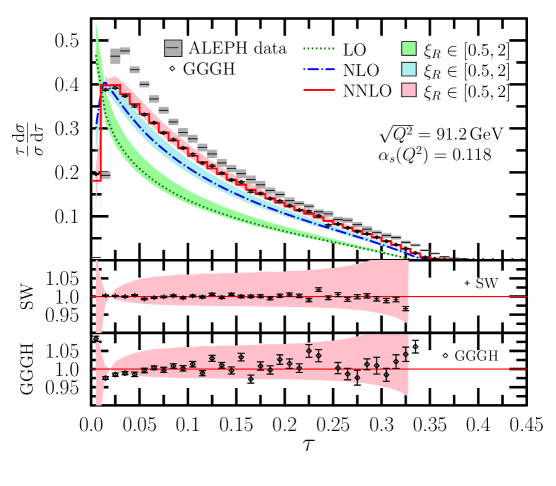
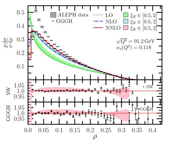
Figure 1: Perturbative predictions for the thrust ($\tau$) and heavy jet mass ($\rho$) distributions at LO, NLO and NNLO accuracy. The bands represent the renormalization scale uncertainty of our predictions corresponding to the range $\xi_{R}\in[0.5,2]$ around the central value of $\mu_{0}=\sqrt{Q^{2}}$. The lower panels show the ratio of the (updated but unpublished – see text) predictions of [6] (SW) and EERAD3 [96] (GGGH) to CoLoRFulNNLO (this work). The bands on the lower panels show the relative scale uncertainty of our NNLO results.

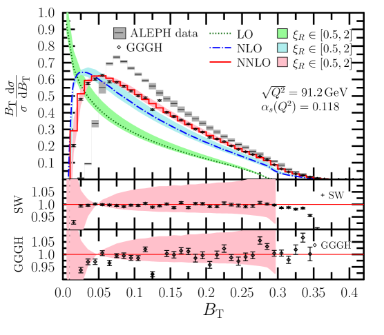
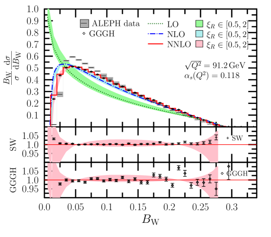
Figure 2: Same as figure 1 for total ($B_{T}$) and wide ($B_{W}$) jet broadening.

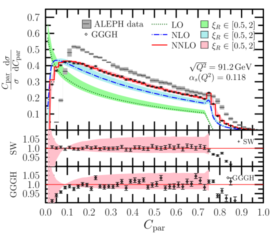
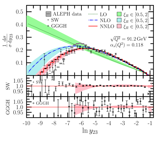
Figure 3: Same as figure 1 for the $C$-parameter ($C_{\rm par}$) and the two-to-three jet transition parameter ($y_{23}$) in the Durham clustering algorithm.

The dependence on the renormalization scale increases significantly beyond kinematical regions of three-parton contributions, for instance for $\tau>1/3$ or $C_{\rm par}>3/4$ and thus those are not shown on the ratio plots. At these three-parton kinematical limits large logarithms appear inside the physical region which have to be resummed similarly to the large logarithms that appear for small values of the event shapes (at the boundary of the physical region) [97].

As mentioned above, predictions for these six event shapes were presented in refs. [5, 6]. In order to quantify the level of agreement across the available perturbative predictions, we also show the ratio of the (updated but unpublished – see below) results of ref. [6] (denoted by SW) and those of EERAD3 (denoted by GGGH) normalized to ours in the middle and bottom panels of each figure. Since the published predictions of [6] are known to be affected by an issue with the phase space generation in the code used to compute those results [98], we have made comparisons to updated but unpublished results which where provided to us by S. Weinzierl. The general conclusion one may draw is that our predictions are in agreement with the updated predictions of SW except for very small and large (beyond the kinematic limits at LO) values of the event shapes, up to the estimated statistical uncertainties. A qualitatively similar statement can be made about the comparison to the GGGH predictions, although the deviations from our results at small values of event shapes are in general more pronounced than for the SW predictions. This is especially apparent for the $C$-parameter distribution below $C_{\rm par}=0.1$.

The level of agreement among the perturbative predictions can be seen better by looking at the NNLO coefficients directly, as shown in figure 4. In the figures the upper panels show the distributions of the NNLO coefficients $O\,C(O)$, while the middle and bottom panels once more present the ratios of the results of SW and those of GGGH normalized to ours. Again we observe a good numerical convergence of our method: the relative uncertainties of the Monte Carlo integrations are shown as shaded bands around the lines at one on the lower panels. The peaks which appear in the relative uncertainties are artifacts of the distributions changing sign with the absolute uncertainties remaining small. The scattered error bars represent the statistical uncertainties of the Monte Carlo integrations of the other two predictions.

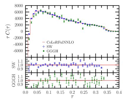
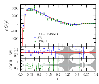
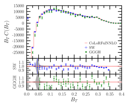
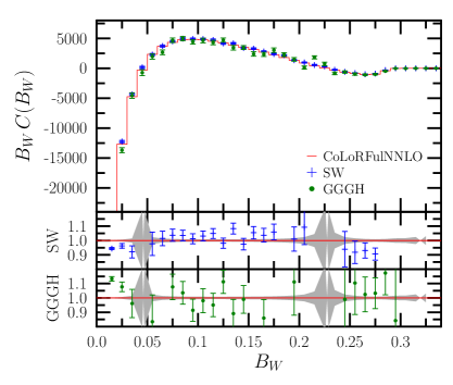
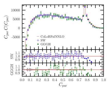
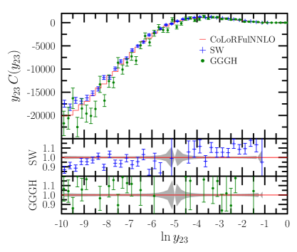
Figure 4: The $O\,C(O)$ coefficients of the thrust, heavy jet mass, total and wide jet broadening, $C$-parameter and two-to-three jet transition variable $y_{23}$ distributions. Lower panels show the ratio of the (updated but unpublished – see text) predictions of [6] (SW) and EERAD3 [96] (GGGH) to CoLoRFulNNLO (this work). The shaded bands on the lower panels represent the relative statistical uncertainties of our predictions due to Monte Carlo integrations.

Examining the plots in figure 4, we see that the agreement is generally quite good between the predictions of SW and CoLoRFulNNLO and reasonably good between GGGH and CoLoRFulNNLO. However the precise comparison to GGGH predictions is hampered by the somewhat large integration uncertainties and bin-to-bin fluctuations of those results. Also, significant deviations among the three predictions are visible for small and large values of the event shapes. For example for $\tau=1-T$ the differences between the CoLoRFulNNLO results and the other two computations grow up to a factor of two for $\tau>1/3$. However, in this region, the contribution from three-particle final states vanishes and the thrust distribution is determined by a four-jet final state. Thus, $C(\tau)$ is determined by the NLO corrections to four-jet production, which have been known for a long time [8, 9] and can also be computed with modern automated tools such as MadGraph5_aMC@NLO [99]. We have checked that our predictions are in complete agreement with those of MadGraph5_aMC@NLO. The same is true for the tails of the other distributions beyond their respective kinematic limits. For small values of the event shapes we have checked that our predictions agree with the resummed predictions obtained from SCET [100, 17, 20] expanded to $\rm O(\alpha_{\rm{s}}^{3})$.

5.3 Jet cone energy fraction

The jet cone energy fraction defined in eq. (5.9) is a particularly simple and excellent observable for the determination of the strong coupling. The smallness of hadronization corrections, detector corrections as well as perturbative corrections allows a specially wide fit range to be used for the extraction of $\alpha_{\rm{s}}$ [90]. JCEF was computed at NLO accuracy for the first time in ref. [89]. Here we present the first result for the JCEF distribution at NNLO accuracy in perturbative QCD for collider energy of $\sqrt{Q^{2}}=91.2$ GeV. In figure 5 we show physical predictions for JCEF, as well as the measured data by the DELPHI collaboration. As previously, the uncertainties due to the variation of the renormalization scale in the range $[0.5,2]$ times our default scale choice (the total center-of-mass energy) are shown as bands on the upper panel. We indicate the relative scale uncertainty at NNLO on the bottom panel.

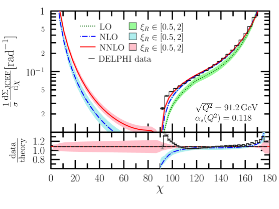
Figure 5: The distribution of jet cone energy fraction (JCEF) at LO, NLO and NNLO accuracy in perturbative QCD. The bands represent the variation of the renormalization scale in the range $\xi_{R}=\mu/\mu_{0}\in[0.5,2]$ around the central value of $\mu_{0}=\sqrt{Q^{2}}$. The lower panel shows the relative scale dependence at NNLO accuracy.

To better appreciate the impact of the NNLO corrections, we show in figure 6 the distribution of the NNLO coefficient $C(\chi)$ directly. Also for these distributions, we observe a good numerical convergence of our code.

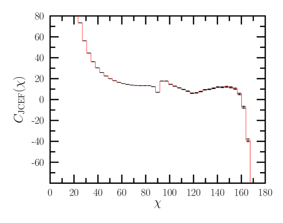
Figure 6: The distribution of the NNLO coefficient for jet cone energy fraction (JCEF). The error bars represent the statistical uncertainty of the Monte Carlo integrations.

6 Conclusions and outlook

In this paper we presented the CoLoRFulNNLO framework to compute higher order radiative corrections to jet cross sections in perturbative QCD. CoLoRFulNNLO is a completely local and fully differential subtraction scheme based on the known infrared factorization properties of QCD matrix elements in soft and collinear limits. Since the subtraction terms explicitly take all color and spin correlations into account, the regularized real emission terms (both double real and real-virtual) are well-defined and can be computed in four dimensions with whatever numerical procedure is deemed most convenient. We have shown analytically that explicit infrared $\epsilon$-poles coming from loop amplitudes cancel against the integrated forms of subtraction terms both in the real-virtual contribution (for any number of jets) and double virtual contribution (with up to three jets in the final state).

We have also reported on the computation of NNLO corrections to three-jet event shape observables in electron-positron collisions using CoLoRFulNNLO. We observe a very good numerical convergence of our method, which we attribute at least in part to the complete locality of the subtraction terms.

We compared both our physical predictions as well as the NNLO contribution only with similar predictions published earlier (in ref. [96] denoted by GGGH and in ref. [6] denoted by SW) for thrust, heavy jet mass, total and wide jet broadening, the C-parameter and the two-to-three jet transition variable $y_{23}$ in the Durham jet clustering algorithm. We find agreement with the updated (unpublished) predictions of SW within the statistical uncertainty of the numerical integrations except for very small and large values of the event shapes, beyond the kinematic limits at LO. The measured data in these regions are limited by statistics and so the phenomenological relevance of the differences is negligible. The same is true for the comparison to the physical predictions of GGGH, however the deviations from our results for small values of event shapes are generally more pronounced than for the predictions of SW. This is especially apparent for small values of the $C$-parameter, below $C_{\rm par}=0.1$. When comparing our physical predictions at the NNLO accuracy to experimental data, we still find large differences. An important source of discrepancy is the neglected large logarithmic contributions which require all-order resummation. Work towards matching the fixed-order predictions to resummed ones is in progress.

Finally, we have shown for the first time perturbative predictions for jet cone energy fraction at NNLO, thereby providing a new observable from which the value of the strong coupling can be extracted at this accuracy. This observable has the remarkable property that the NNLO corrections are very small and the fairly good agreement between data and predictions already at NLO become only marginally better with the inclusion of the NNLO corrections. This stability of the perturbative predictions makes JCEF a good candidate for the extraction of the strong coupling.

We emphasize that our framework is not restricted to three-jet production, but it can be easily applied to study differential distributions for four- or more jet production once the necessary two-loop matrix elements become available. CoLoRFulNNLO is completely worked out for processes with colorless initial states at present. The inclusion of initial state radiation is a conceptually straightforward although substantial task and is work in progress.

Note added

After the completion of this manuscript, we were provided new predictions of EERAD3 by G. Heinrich. In the present version of this paper, we have made comparisons to these unpublished new predictions.

Appendix A The ${\mbox{\boldmath$I$}}_{1}^{(0)}$ insertion operator up to $\rm O(\epsilon)$

We present the Laurent expansion of the kinematic functions that appear in the ${\mbox{\boldmath$I$}}_{1}^{(0)}(\{p\}_{m};\epsilon)$ insertion operator in eq. (3.9) up to and including $\rm O(\epsilon)$ terms. An expansion to this order is sufficient for demonstrating the cancellation of the $\epsilon$-poles at NNLO. We have also computed the $\rm O(\epsilon^{2})$ coefficients of the expansions analytically, however they are quite lengthy and we do not display them here.

The ${{\rm C}}_{1,i}^{(0)}(x,\epsilon)$ are obtained as the following combination of terms

$${{\rm C}}_{1,q}^{(0)}(x,\epsilon) =[{{\rm C}}_{ir}^{(0)}]_{qg}(x,\epsilon)-[{{\rm C}}_{ir}{{\rm S}}_{r}^{(0)}](\epsilon)\,,$$ (A.1)

$${{\rm C}}_{1,g}^{(0)}(x,\epsilon) =\frac{1}{2}[{{\rm C}}_{ir}^{(0)}]_{gg}(x,\epsilon)+n_{\rm{f}}[{{\rm C}}_{ir}^{(0)}]_{q{\bar{q}}}(x,\epsilon)-[{{\rm C}}_{ir}{{\rm S}}_{r}^{(0)}](\epsilon)\,,$$ (A.2)

where

$$[{{\rm C}}_{ir}^{(0)}]_{qg}(x;\epsilon,\alpha_{0}=1,d_{0}=3-3\epsilon)=\frac{1}{\epsilon^{2}}+\left(\frac{3}{2}-2\ln(x)\right)\frac{1}{\epsilon}$$

$$\quad+2\left(1+\frac{1}{(1-x)^{5}}\right){\rm Li}_{2}(1-x)-\frac{\pi^{2}}{2}+2\ln^{2}(x)$$

$$\quad+\left(\frac{8}{3(1-x)^{5}}-\frac{3}{2(1-x)^{4}}-\frac{1}{3(1-x)^{3}}+\frac{1}{3(1-x)^{2}}+\frac{3}{2(1-x)}-\frac{17}{3}\right)\ln(x)$$

$$\quad+\frac{2}{3(1-x)^{4}}-\frac{2}{3(1-x)^{3}}-\frac{5}{12(1-x)^{2}}+\frac{5}{24(1-x)}+\frac{89}{24}$$

$$\quad+\epsilon\,\Bigg{[}\left(10+\frac{26}{(1-x)^{5}}\right){\rm Li}_{3}(1-x)+20\left(1+\frac{1}{(1-x)^{5}}\right)\left({\rm Li}_{3}(x)-\zeta_{3}\right)$$

$$\qquad+8\left(1+\frac{1}{(1-x)^{5}}\right)\ln(x){\rm Li}_{2}(1-x)$$

$$\qquad-\frac{4\ln^{3}(x)}{3}+10\left(1+\frac{1}{(1-x)^{5}}\right)\ln(1-x)\ln^{2}(x)-\left(1+\frac{2}{(1-x)^{5}}\right)\pi^{2}\ln(x)$$

$$\qquad-\left(\frac{31}{3(1-x)^{5}}+\frac{1}{2(1-x)^{4}}+\frac{7}{3(1-x)^{3}}+\frac{13}{3(1-x)^{2}}+\frac{19}{2(1-x)}-\frac{17}{3}\right){\rm Li}_{2}(1-x)$$

$$\qquad-\left(\frac{8}{3(1-x)^{5}}-\frac{3}{2(1-x)^{4}}-\frac{1}{3(1-x)^{3}}+\frac{1}{3(1-x)^{2}}+\frac{3}{2(1-x)}-\frac{17}{3}\right)\ln^{2}(x)$$

$$\qquad+\left(\frac{4}{3(1-x)^{4}}+\frac{2}{3(1-x)^{3}}+\frac{4}{9(1-x)^{2}}+\frac{1}{3(1-x)}+\frac{37}{36}\right)\pi^{2}$$

$$\qquad+\left(\frac{1793}{72(1-x)^{5}}-\frac{123}{8(1-x)^{4}}-\frac{41}{36(1-x)^{3}}+\frac{119}{36(1-x)^{2}}+\frac{109}{8(1-x)}-\frac{2327}{72}\right)\ln(x)$$

$$\qquad+\frac{665}{72(1-x)^{4}}-\frac{1069}{144(1-x)^{3}}-\frac{343}{144(1-x)^{2}}+\frac{737}{144(1-x)}+\frac{353}{144}\Bigg{]}+\rm O(\epsilon^{2})\,,$$ (A.3)

$$[{{\rm C}}_{ir}^{(0)}]_{q{\bar{q}}}(x;\epsilon,\alpha_{0}=1,d_{0}=3-3\epsilon)=\frac{T_{\rm{R}}}{C_{\rm{A}}}\Bigg{\{}-\frac{2}{3\epsilon}$$

$$\quad+\frac{2}{3}\left(1+\frac{1}{(1-x)^{5}}\right)\ln(x)-\frac{160}{3}\left(\frac{2}{(2-x)^{6}}-\frac{1}{(2-x)^{5}}\right)\ln\left(\frac{x}{2}\right)$$

$$\quad+\frac{2}{3(1-x)^{4}}+\frac{1}{3(1-x)^{3}}+\frac{2}{9(1-x)^{2}}+\frac{1}{6(1-x)}-\frac{5}{2}$$

$$\quad-\frac{160}{3(2-x)^{5}}+\frac{40}{3(2-x)^{4}}+\frac{20}{9(2-x)^{3}}+\frac{5}{9(2-x)^{2}}+\frac{1}{6(2-x)}$$

$$\quad+\epsilon\,\Bigg{[}-\left(\frac{14}{3(1-x)^{5}}+\frac{2}{3}\right){\rm Li}_{2}(1-x)-\frac{2}{3}\left(1+\frac{1}{(1-x)^{5}}\right)\ln^{2}(x)$$

$$\qquad+\frac{160}{3}\left(\frac{2}{(2-x)^{6}}-\frac{1}{(2-x)^{5}}\right)\left(8{\rm Li}_{2}\left(1-\frac{x}{2}\right)-{\rm Li}_{2}(1-x)+\ln^{2}\left(\frac{x}{2}\right)\right)$$

$$\qquad+\frac{7}{9}\pi^{2}-\frac{40}{9}\left(\frac{2}{(2-x)^{6}}-\frac{1}{(2-x)^{5}}\right)\pi^{2}+\frac{992}{9}\left(\frac{2}{(2-x)^{6}}-\frac{1}{(2-x)^{5}}\right)\ln(2)$$

$$\qquad+\bigg{(}\frac{5}{2(1-x)^{5}}-\frac{1}{(1-x)^{4}}-\frac{17}{18(1-x)^{3}}-\frac{11}{6(1-x)^{2}}-\frac{9}{(1-x)}+\frac{5}{2}$$

$$\qquad\quad-\frac{1984}{9(2-x)^{6}}+\frac{1952}{9(2-x)^{5}}+\frac{80}{9(2-x)^{3}}+\frac{80}{9(2-x)^{2}}+\frac{8}{(2-x)}\bigg{)}\ln(x)$$

$$\qquad+\frac{43}{6(1-x)^{4}}+\frac{25}{12(1-x)^{3}}+\frac{31}{54(1-x)^{2}}-\frac{10}{9(1-x)}-\frac{1399}{108}$$

$$\qquad-\frac{4832}{9(2-x)^{5}}+\frac{1688}{9(2-x)^{4}}+\frac{644}{27(2-x)^{3}}+\frac{176}{27(2-x)^{2}}+\frac{25}{9(2-x)}\Bigg{]}\Bigg{\}}+\rm O(\epsilon^{2})\,,$$ (A.4)

$$[{{\rm C}}_{ir}^{(0)}]_{gg}(x;\epsilon,\alpha_{0}=1,d_{0}=3-3\epsilon)=\frac{2}{\epsilon^{2}}+\left(\frac{11}{3}-4\ln(x)\right)\frac{1}{\epsilon}$$

$$\quad+4\left(1+\frac{1}{(1-x)^{5}}\right){\rm Li}_{2}(1-x)+4\ln^{2}(x)-\pi^{2}+\frac{160}{3}\left(\frac{2}{(2-x)^{6}}-\frac{1}{(2-x)^{5}}\right)\ln\left(\frac{x}{2}\right)$$

$$\quad+\left(\frac{14}{3(1-x)^{5}}-\frac{3}{(1-x)^{4}}-\frac{2}{3(1-x)^{3}}+\frac{2}{3(1-x)^{2}}+\frac{3}{1-x}-12\right)\ln(x)$$

$$\quad+\frac{2}{3(1-x)^{4}}-\frac{5}{3(1-x)^{3}}-\frac{19}{18(1-x)^{2}}+\frac{1}{4(1-x)}+\frac{37}{4}$$

$$\quad+\frac{160}{3(2-x)^{5}}-\frac{40}{3(2-x)^{4}}-\frac{20}{9(2-x)^{3}}-\frac{5}{9(2-x)^{2}}-\frac{1}{6(2-x)}$$

$$\quad+\epsilon\Bigg{[}40\left(1+\frac{1}{(1-x)^{5}}\right)\left({\rm Li}_{3}(x)-\zeta_{3}\right)+\left(20+\frac{52}{(1-x)^{5}}\right){\rm Li}_{3}(1-x)-\frac{8\ln^{3}(x)}{3}$$

$$\qquad+16\left(1+\frac{1}{(1-x)^{5}}\right)\ln(x){\rm Li}_{2}(1-x)+20\left(1+\frac{1}{(1-x)^{5}}\right)\ln(1-x)\ln^{2}(x)$$

$$\qquad-2\left(1+\frac{2}{(1-x)^{5}}\right)\pi^{2}\ln(x)$$

$$\qquad-\left(\frac{16}{(1-x)^{5}}+\frac{1}{(1-x)^{4}}+\frac{14}{3(1-x)^{3}}+\frac{26}{3(1-x)^{2}}+\frac{19}{1-x}-12\right){\rm Li}_{2}(1-x)$$

$$\qquad-\frac{160}{3}\left(\frac{2}{(2-x)^{6}}-\frac{1}{(2-x)^{5}}\right)\left(8{\rm Li}_{2}\left(1-\frac{x}{2}\right)-{\rm Li}_{2}(1-x)+\ln^{2}\left(\frac{x}{2}\right)\right)$$

$$\qquad-\left(\frac{14}{3(1-x)^{5}}-\frac{3}{(1-x)^{4}}-\frac{2}{3(1-x)^{3}}+\frac{2}{3(1-x)^{2}}+\frac{3}{1-x}-12\right)\ln^{2}(x)$$

$$\qquad+\left(\frac{8}{3(1-x)^{4}}+\frac{4}{3(1-x)^{3}}+\frac{8}{9(1-x)^{2}}+\frac{2}{3(1-x)}+\frac{23}{18}\right)\pi^{2}$$

$$\qquad+\frac{40}{9}\left(\frac{2}{(2-x)^{6}}-\frac{1}{(2-x)^{5}}\right)\pi^{2}-\frac{512}{9}\left(\frac{2}{(2-x)^{6}}-\frac{1}{(2-x)^{5}}\right)\ln(2)$$

$$\qquad+\bigg{(}\frac{1727}{36(1-x)^{5}}-\frac{119}{4(1-x)^{4}}-\frac{4}{3(1-x)^{3}}+\frac{76}{9(1-x)^{2}}+\frac{145}{4(1-x)}-\frac{2393}{36}$$

$$\qquad\quad+\frac{1024}{9(2-x)^{6}}-\frac{1472}{9(2-x)^{5}}-\frac{80}{9(2-x)^{3}}-\frac{80}{9(2-x)^{2}}-\frac{8}{2-x}\bigg{)}\ln(x)$$

$$\qquad+\frac{431}{36(1-x)^{4}}-\frac{1195}{72(1-x)^{3}}-\frac{1105}{216(1-x)^{2}}+\frac{829}{72(1-x)}+\frac{3317}{216}$$

$$\qquad+\frac{4352}{9(2-x)^{5}}-\frac{1568}{9(2-x)^{4}}-\frac{584}{27(2-x)^{3}}-\frac{161}{27(2-x)^{2}}-\frac{47}{18(2-x)}\Bigg{]}+\rm O(\epsilon^{2})\,,$$ (A.5)

and

$$[{{\rm C}}_{ir}{{\rm S}}_{r}^{(0)}](\epsilon,1,3-3\epsilon)=\frac{1}{\epsilon^{2}}+\frac{11}{3\epsilon}-\frac{7}{6}\pi^{2}+\frac{329}{18}+\left(-32\zeta(3)-\frac{77}{18}\pi^{2}+\frac{9779}{108}\right)\epsilon+\rm O(\epsilon^{2})\,.$$ (A.6)

The integrated soft kinematic function ${{\rm S}}_{1}^{(0),(i,k)}(Y,\epsilon)$ is simply given by

$${{\rm S}}_{1}^{(0),(i,k)}(Y,\epsilon)=[{{\rm S}}_{1}^{(0)}]^{(i,k)}(Y,\epsilon)\,,$$ (A.7)

where

$$[{{\rm S}}_{r}^{(0)}]^{(i,k)}(Y;\epsilon,y_{0}=1,d_{0}^{\prime}=3-3\epsilon)=-\frac{1}{\epsilon^{2}}+\left(\ln(Y)-\frac{11}{3}\right)\frac{1}{\epsilon}$$

$$\qquad-{\rm Li}_{2}(1-Y)-\frac{1}{2}\ln^{2}(Y)+\frac{7}{6}\pi^{2}+\frac{11}{3}\ln(Y)-\frac{317}{18}$$

$$\qquad+\bigg{[}-{\rm Li}_{3}(1-Y)-{\rm Li}_{3}(Y)+\frac{1}{6}\ln^{3}(Y)-\frac{1}{2}\ln(1-Y)\ln^{2}(Y)-\pi^{2}\ln(Y)+33\zeta(3)$$

$$\qquad+\frac{11}{6}\left(-2{\rm Li}_{2}(1-Y)-\ln^{2}(Y)+\frac{7}{3}\pi^{2}\right)+\frac{317\ln(Y)}{18}-\frac{9299}{108}\bigg{]}\epsilon+\rm O(\epsilon^{2})\,.$$ (A.8)

Appendix B Asymptotic form of the ${\mbox{\boldmath$J$}}_{2}$ insertion operator

We defined the ${\mbox{\boldmath$J$}}_{2}$ insertion operator in eq. (4.26) and exhibited its pole structure for three hard partons in the final state in eq. (4.27). That is sufficient to check the cancellation of the double virtual $\epsilon$-poles at NNLO. However, in the numerical integrations over the three-parton phase space one also needs the finite part, which is rather lengthy and in fact, we have only computed its asymptotic expansion for small kinematic invariants analytically. Here we record this expansion and comment on the remaining regular part, which we compute numerically.

For the Born process $e^{+}e^{-}\to q{\bar{q}}g$ the ${\mbox{\boldmath$J$}}_{2}$ operator can be written in the following explicit form:

$$\begin{split}{\mbox{\boldmath$J$}}_{2}(\epsilon)=&\left[\frac{\alpha_{\rm{s}}}{2\pi}\frac{S_{\epsilon}}{S_{\epsilon}^{\overline{\rm{MS}}}}\left(\frac{\mu^{2}}{Q^{2}}\right)^{\epsilon}\right]^{2}\Bigg{\{}\frac{1}{\epsilon^{3}}(C_{\rm{A}}+2C_{\rm{F}})\Bigg{(}-\frac{3}{8}\beta_{0}\Bigg{)}\\ &+\frac{1}{\epsilon^{2}}\Bigg{[}\frac{1}{4}\beta_{0}\bigg{(}C_{\rm{A}}(\ln y_{13}+\ln y_{23})-(C_{\rm{A}}-2C_{\rm{F}})\ln y_{12}\bigg{)}-\frac{\pi^{2}}{24}C_{\rm{A}}(C_{\rm{A}}+2C_{\rm{F}})\\ &\qquad-\frac{3}{4}C_{\rm{A}}^{2}-\frac{8}{9}C_{\rm{A}}C_{\rm{F}}+\frac{17}{18}C_{\rm{A}}n_{\rm{f}}T_{\rm{R}}+\frac{4}{9}C_{\rm{F}}n_{\rm{f}}T_{\rm{R}}-\frac{2}{9}n_{\rm{f}}^{2}T_{\rm{R}}^{2}\Bigg{]}\\ &+\frac{1}{\epsilon}\Bigg{[}-\frac{K}{2}\bigg{(}C_{\rm{A}}(\ln y_{13}+\ln y_{23})-(C_{\rm{A}}-2C_{\rm{F}})\ln y_{12}\bigg{)}\\ &\qquad-\bigg{(}\frac{11}{36}C_{\rm{A}}^{2}+\frac{1}{2}C_{\rm{F}}^{2}-\frac{1}{9}C_{\rm{A}}n_{\rm{f}}T_{\rm{R}}\bigg{)}\pi^{2}-\bigg{(}\frac{1}{4}C_{\rm{A}}^{2}+\frac{13}{2}C_{\rm{A}}C_{\rm{F}}-6C_{\rm{F}}^{2}\bigg{)}\zeta(3)\\ &\qquad+\frac{173}{54}C_{\rm{A}}^{2}+\frac{961}{216}C_{\rm{A}}C_{\rm{F}}-\frac{32}{27}C_{\rm{A}}n_{\rm{f}}T_{\rm{R}}+\frac{3}{8}C_{\rm{F}}^{2}-\frac{46}{27}C_{\rm{F}}n_{\rm{f}}T_{\rm{R}}\Bigg{]}\Bigg{\}}\\ &+{\cal F}in\Big{(}{\mbox{\boldmath$J$}}_{2}(\epsilon)\Big{)}+\rm O(\epsilon)\,,\end{split}$$ (B.1)

which then also defines the finite part ${\cal F}in\Big{(}{\mbox{\boldmath$J$}}_{2}(\epsilon)\Big{)}$ unambiguously. We decompose the finite part into an asymptotic piece which collects all logarithmic contributions that become singular on the borders of the three-parton phase space and a piece which is regular over the whole phase space, i.e. finite on the borders:

$${\cal F}in\Big{(}{\mbox{\boldmath$J$}}_{2}(\epsilon)\Big{)}={\cal F}in\Big{(}{\mbox{\boldmath$J$}}_{2}^{\mathrm{asy}}(\epsilon)\Big{)}+{\cal F}in\Big{(}{\mbox{\boldmath$J$}}_{2}^{\mathrm{reg}}(\epsilon)\Big{)}\,.$$ (B.2)

The asymptotic part can be written as

$$\begin{split}{\cal F}in\Big{(}{\mbox{\boldmath$J$}}_{2}^{\mathrm{asy}}(\epsilon)\Big{)}&=\left[\frac{\alpha_{\rm{s}}}{2\pi}\frac{S_{\epsilon}}{S_{\epsilon}^{\overline{\rm{MS}}}}\left(\frac{\mu^{2}}{Q^{2}}\right)^{\epsilon}\right]^{2}\\ &\times\sum_{i=1}^{3}\bigg{[}{{\rm C}}_{2,i}^{\mathrm{asy}}(x_{i})\left({\mbox{\boldmath$T$}}_{i}^{2}\right)^{2}+\sum_{\begin{subarray}{c}k=1\\ k\neq i\end{subarray}}^{3}\bigg{(}{{\rm S}}_{2}^{\mathrm{asy}}(Y_{ik})\,C_{\rm{A}}+{\rm C}\kern-2.0pt{\rm S}_{2,i}^{\mathrm{asy}}(x_{i},Y_{ik})\,{\mbox{\boldmath$T$}}_{i}^{2}\bigg{)}{\mbox{\boldmath$T$}}_{i}\!\cdot\!{\mbox{\boldmath$T$}}_{k}\bigg{]}\,.\end{split}$$ (B.3)

We stress that this form as well as the explicit expressions for the asymptotic functions presented below are known to be appropriate only for $e^{+}e^{-}\to 3$ jet production. The analytic expressions for the asymptotic parts of the kinematic functions read as follows:

$${{\rm C}}_{2,q}^{\mathrm{asy}}(x)= -\frac{1}{9}\pi^{2}\ln(x)+12\zeta(3)\ln(x)-\frac{27\ln(x)}{4}+\frac{C_{\rm{A}}}{C_{\rm{F}}}\bigg{[}-\frac{22\ln^{3}(x)}{9}-\frac{1}{3}\pi^{2}\ln^{2}(x)$$

$$+\frac{233\ln^{2}(x)}{18}-3\zeta(3)\ln(x)-4\pi^{2}\ln(2)\ln(x)+\frac{7}{12}\pi^{2}\ln(x)-\frac{2239\ln(x)}{108}\bigg{]}$$

$$+n_{\rm{f}}\frac{T_{\rm{R}}}{C_{\rm{F}}}\bigg{[}\frac{8\ln^{3}(x)}{9}-\frac{38}{9}\ln^{2}(x)+\frac{\pi^{2}}{3}\ln(x)+\frac{137\ln(x)}{27}\bigg{]}\,,$$ (B.4)

$${{\rm C}}_{2,g}^{\mathrm{asy}}(x)= -\frac{22}{9}\ln^{3}(x)-\frac{1}{3}\pi^{2}\ln^{2}(x)+\frac{85\ln^{2}(x)}{6}+9\zeta(3)\ln(x)-4\pi^{2}\ln(2)\ln(x)+\frac{37}{36}\pi^{2}\ln(x)$$

$$-\frac{884\ln(x)}{27}+n_{\rm{f}}\frac{T_{\rm{R}}}{C_{\rm{A}}}\bigg{[}\frac{8\ln^{3}(x)}{9}-\frac{64\ln^{2}(x)}{9}+\frac{5}{9}\pi^{2}\ln(x)+\frac{107\ln(x)}{9}\bigg{]}$$

$$+n_{\rm{f}}\frac{C_{\rm{F}}T_{\rm{R}}}{C_{\rm{A}}^{2}}\bigg{[}-\frac{4}{3}\pi^{2}\ln(x)+\frac{14\ln(x)}{3}\bigg{]}+n_{\rm{f}}^{2}\frac{T_{\rm{R}}^{2}}{C_{\rm{A}}^{2}}\bigg{[}\frac{8\ln^{2}(x)}{9}-\frac{52\ln(x)}{27}\bigg{]}\,,$$ (B.5)

$${{\rm S}}_{2}^{\mathrm{asy}}(Y) =\frac{11\ln^{3}(Y)}{18}+\frac{13}{6}\pi^{2}\ln^{2}(Y)-\frac{244\ln^{2}(Y)}{9}+17\zeta(3)\ln(Y)-8\ln^{2}(2)\ln(Y)-\frac{13}{4}\pi^{2}\ln(Y)$$

$$+\frac{217}{9}\ln(2)\ln(Y)+\frac{131167\ln(Y)}{2700}+\frac{C_{\rm{F}}}{C_{\rm{A}}}\bigg{[}-\frac{4}{3}\pi^{2}\ln^{2}(Y)+\frac{98\ln^{2}(Y)}{9}-16\zeta(3)\ln(Y)$$

$$+\frac{26}{3}\pi^{2}\ln(Y)-\frac{5099\ln(Y)}{75}\bigg{]}+n_{\rm{f}}\frac{T_{\rm{R}}}{C_{\rm{A}}}\bigg{[}-\frac{2}{9}\ln^{3}(Y)+\frac{20\ln^{2}(Y)}{9}+16\ln^{2}(2)\ln(Y)$$

$$-\frac{29}{9}\pi^{2}\ln(Y)-\frac{434}{9}\ln(2)\ln(Y)+\frac{4279\ln(Y)}{135}\bigg{]}\,,$$ (B.6)

$${\rm C}\kern-2.0pt{\rm S}_{2,q}^{\mathrm{asy}}(x,Y) =8\bigg{(}\frac{1}{(1-x)^{5}}+1\bigg{)}\bigg{(}2{\rm Li}_{3}(1-x)\ln(Y)+{\rm Li}_{2}(1-x)\ln(x)\ln(Y)$$

$$+2{\rm Li}_{3}(x)\ln(Y)+\ln(1-x)\ln^{2}(x)\ln(Y)-\frac{\pi^{2}}{6}\ln(x)\ln(Y)-2\zeta(3)\ln(Y)\bigg{)}$$

$$-8\bigg{(}{\rm Li}_{3}(1-x)\ln(Y)-{\rm Li}_{2}(1-Y)\ln(x)\ln(Y)-{\rm Li}_{3}(1-Y)\ln(x)-2{\rm Li}_{3}(Y)\ln(x)$$

$$-\ln(x)\ln(1-Y)\ln^{2}(Y)+\frac{\pi^{2}}{3}\ln(x)\ln(Y)-\frac{\pi^{2}}{6}\ln^{2}(Y)-4\zeta(3)\ln(Y)\bigg{)}$$

$$-\frac{4}{3}\bigg{(}2{\rm Li}_{2}(1-Y)\ln(x)+\ln(x)\ln^{2}(Y)\bigg{)}-\bigg{(}\frac{38}{3(1-x)^{5}}-\frac{2}{(1-x)^{4}}+\frac{2}{(1-x)^{3}}$$

$$+\frac{4}{(1-x)^{2}}+\frac{8}{1-x}-\frac{16}{3}\bigg{)}{\rm Li}_{2}(1-x)\ln(Y)-\frac{107\ln^{2}(Y)}{9}+\bigg{(}\frac{4}{3(1-x)^{4}}$$

$$+\frac{2}{3(1-x)^{3}}+\frac{4}{9(1-x)^{2}}+\frac{1}{3(1-x)}-4\bigg{)}\pi^{2}\ln(Y)+\bigg{(}\frac{157}{18(1-x)^{5}}-\frac{5}{3(1-x)^{4}}$$

$$-\frac{53}{18(1-x)^{3}}+\frac{16}{9(1-x)^{2}}+\frac{35}{3(1-x)}-\frac{104}{9}\bigg{)}\ln(x)\ln(Y)+\frac{4}{1-Y}\ln(x)\ln(Y)$$

$$+\bigg{(}\frac{97}{18(1-x)^{4}}-\frac{77}{36(1-x)^{3}}-\frac{17}{9(1-x)^{2}}+\frac{145}{36(1-x)}+\frac{9247}{450}\bigg{)}\ln(Y)$$

$$+\frac{C_{\rm{A}}}{C_{\rm{F}}}\bigg{[}-\frac{4}{3}\pi^{2}\ln^{2}(Y)+\frac{35\ln^{2}(Y)}{3}-16\zeta(3)\ln(Y)+\frac{22}{9}\pi^{2}\ln(Y)+8\ln^{2}(2)\ln(Y)$$

$$-\frac{224}{9}\ln(2)\ln(Y)+\frac{9629\ln(Y)}{1350}\bigg{]}+n_{\rm{f}}\frac{T_{\rm{R}}}{C_{\rm{F}}}\bigg{[}\frac{4\ln^{2}(Y)}{9}+\frac{28}{9}\pi^{2}\ln(Y)-16\ln^{2}(2)\ln(Y)$$

$$+\frac{448}{9}\ln(2)\ln(Y)-\frac{7474\ln(Y)}{135}\bigg{]}\,,$$ (B.7)

and

$${\rm C}\kern-2.0pt{\rm S}_{2,g}^{\mathrm{asy}}(x,Y) =8\bigg{(}\frac{1}{(1-x)^{5}}+1\bigg{)}\bigg{(}2{\rm Li}_{3}(1-x)\ln(Y)+{\rm Li}_{2}(1-x)\ln(x)\ln(Y)$$

$$+2{\rm Li}_{3}(x)\ln(Y)+\ln(1-x)\ln^{2}(x)\ln(Y)-\frac{\pi^{2}}{6}\ln(x)\ln(Y)-2\zeta(3)\ln(Y)\bigg{)}$$

$$-8\bigg{(}{\rm Li}_{3}(1-x)\ln(Y)-{\rm Li}_{2}(1-Y)\ln(x)\ln(Y)-{\rm Li}_{3}(1-Y)\ln(x)$$

$$-2{\rm Li}_{3}(Y)\ln(x)-\ln(x)\ln(1-Y)\ln^{2}(Y)+\frac{\pi^{2}}{3}\ln(x)\ln(Y)-2\zeta(3)\ln(Y)\bigg{)}$$

$$-\frac{4}{3}\bigg{(}2{\rm Li}_{2}(1-Y)\ln(x)+\ln(x)\ln^{2}(Y)\bigg{)}-\bigg{(}\frac{34}{3(1-x)^{5}}-\frac{2}{(1-x)^{4}}$$

$$+\frac{2}{(1-x)^{3}}+\frac{4}{(1-x)^{2}}+\frac{8}{1-x}-\frac{16}{3}\bigg{)}{\rm Li}_{2}(1-x)\ln(Y)-\frac{320}{3}\bigg{(}\frac{2}{(2-x)^{6}}$$

$$-\frac{1}{(2-x)^{5}}\bigg{)}{\rm Li}_{2}\bigg{(}1-\frac{x}{2}\bigg{)}\ln(Y)+\bigg{(}\frac{4}{3(1-x)^{4}}+\frac{2}{3(1-x)^{3}}+\frac{4}{9(1-x)^{2}}$$

$$+\frac{1}{3(1-x)}\bigg{)}\pi^{2}\ln(Y)+\bigg{(}\frac{163}{18(1-x)^{5}}-\frac{7}{3(1-x)^{4}}-\frac{55}{18(1-x)^{3}}+\frac{16}{9(1-x)^{2}}$$

$$+\frac{35}{3(1-x)}-\frac{100}{9}\bigg{)}\ln(x)\ln(Y)-\bigg{(}\frac{96}{(2-x)^{6}}-\frac{272}{3(2-x)^{5}}+\frac{56}{3(2-x)^{4}}$$

$$+\frac{4}{3(2-x)^{3}}\bigg{)}\ln\bigg{(}\frac{x}{2}\bigg{)}\ln(Y)+\frac{4}{1-Y}\ln(x)\ln(Y)+\bigg{(}\frac{79}{18(1-x)^{4}}-\frac{107}{36(1-x)^{3}}$$

$$-\frac{64}{27(1-x)^{2}}+\frac{15}{4(1-x)}\bigg{)}\ln(Y)+\bigg{(}\frac{176}{3(2-x)^{5}}-\frac{20}{3(2-x)^{4}}-\frac{154}{27(2-x)^{3}}$$

$$-\frac{37}{27(2-x)^{2}}-\frac{5}{18(2-x)}\bigg{)}\ln(Y)$$

$$+n_{\rm{f}}\frac{T_{\rm{R}}}{C_{\rm{A}}}\bigg{[}\frac{640}{3}\bigg{(}\frac{2}{(2-x)^{6}}-\frac{1}{(2-x)^{5}}\bigg{)}{\rm Li}_{2}\bigg{(}1-\frac{x}{2}\bigg{)}\ln(Y)$$

$$-\frac{8}{3(1-x)^{5}}{\rm Li}_{2}(1-x)\ln(Y)-\bigg{(}\frac{2}{3(1-x)^{5}}-\frac{4}{3(1-x)^{4}}-\frac{2}{9(1-x)^{3}}$$

$$+\frac{8}{9}\bigg{)}\ln(x)\ln(Y)+\bigg{(}\frac{192}{(2-x)^{6}}-\frac{544}{3(2-x)^{5}}+\frac{112}{3(2-x)^{4}}$$

$$+\frac{8}{3(2-x)^{3}}\bigg{)}\ln\bigg{(}\frac{x}{2}\bigg{)}\ln(Y)+\bigg{(}\frac{2}{(1-x)^{4}}+\frac{5}{3(1-x)^{3}}+\frac{26}{27(1-x)^{2}}$$

$$+\frac{5}{9(1-x)}\bigg{)}\ln(Y)-\bigg{(}\frac{352}{3(2-x)^{5}}-\frac{40}{3(2-x)^{4}}-\frac{308}{27(2-x)^{3}}$$

$$-\frac{74}{27(2-x)^{2}}-\frac{5}{9(2-x)}\bigg{)}\ln(Y)\bigg{]}\,.$$ (B.8)

We do not have analytic expressions for the regular part. However, computing this piece numerically on a grid over the three-parton phase space, we find that it is in fact flat across the whole phase space (within the uncertainty of the numerical integrations). Hence it can be described by a single number whose numerical value we find to be

$${\cal F}in\Big{(}{\mbox{\boldmath$J$}}_{2}^{\mathrm{reg}}(\epsilon)\Big{)}=\left[\frac{\alpha_{\rm{s}}}{2\pi}\frac{S_{\epsilon}}{S_{\epsilon}^{\overline{\rm{MS}}}}\left(\frac{\mu^{2}}{Q^{2}}\right)^{\epsilon}\right]^{2}\bigg{(}-650\bigg{)}$$ (B.9)

for $N_{\rm{c}}=3$, $T_{\rm{R}}=1/2$ and $n_{\rm{f}}=5$.

References

- [1] ALEPH Collaboration, A. Heister et al., “Studies of QCD at e+ e- centre-of-mass energies between 91-GeV and 209-GeV,” Eur.Phys.J. C35 (2004) 457–486.
- [2] DELPHI Collaboration, J. Abdallah et al., “A Study of the energy evolution of event shape distributions and their means with the DELPHI detector at LEP,” Eur.Phys.J. C29 (2003) 285–312, arXiv:hep-ex/0307048 [hep-ex].
- [3] L3 Collaboration, P. Achard et al., “Studies of hadronic event structure in annihilation from 30-GeV to 209-GeV with the L3 detector,” Phys.Rept. 399 (2004) 71–174, arXiv:hep-ex/0406049 [hep-ex].
- [4] OPAL Collaboration, G. Abbiendi et al., “Measurement of event shape distributions and moments in e+ e- hadrons at 91-GeV - 209-GeV and a determination of alpha(s),” Eur.Phys.J. C40 (2005) 287–316, arXiv:hep-ex/0503051 [hep-ex].
- [5] A. Gehrmann-De Ridder, T. Gehrmann, E. Glover, and G. Heinrich, “NNLO corrections to event shapes in e+ e- annihilation,” JHEP 0712 (2007) 094, arXiv:0711.4711 [hep-ph].
- [6] S. Weinzierl, “Event shapes and jet rates in electron-positron annihilation at NNLO,” JHEP 0906 (2009) 041, arXiv:0904.1077 [hep-ph].
- [7] V. Del Duca, C. Duhr, A. Kardos, G. Somogyi, and Z. Trócsányi, “Three-jet production in electron-positron collisions using the CoLoRFulNNLO method,” arXiv:1603.08927 [hep-ph].
- [8] A. Signer and L. J. Dixon, “Electron - positron annihilation into four jets at next-to-leading order in alpha-s,” Phys. Rev. Lett. 78 (1997) 811–814, arXiv:hep-ph/9609460 [hep-ph].
- [9] Z. Nagy and Z. Trocsanyi, “Next-to-leading order calculation of four jet shape variables,” Phys. Rev. Lett. 79 (1997) 3604–3607, arXiv:hep-ph/9707309 [hep-ph].
- [10] J. M. Campbell, M. A. Cullen, and E. W. N. Glover, “Four jet event shapes in electron - positron annihilation,” Eur. Phys. J. C9 (1999) 245–265, arXiv:hep-ph/9809429 [hep-ph].
- [11] S. Weinzierl and D. A. Kosower, “QCD corrections to four jet production and three jet structure in e+ e- annihilation,” Phys. Rev. D60 (1999) 054028, arXiv:hep-ph/9901277 [hep-ph].
- [12] R. Frederix, S. Frixione, K. Melnikov, and G. Zanderighi, “NLO QCD corrections to five-jet production at LEP and the extraction of ,” JHEP 11 (2010) 050, arXiv:1008.5313 [hep-ph].
- [13] S. Becker, D. Goetz, C. Reuschle, C. Schwan, and S. Weinzierl, “NLO results for five, six and seven jets in electron-positron annihilation,” Phys. Rev. Lett. 108 (2012) 032005, arXiv:1111.1733 [hep-ph].
- [14] S. Catani, L. Trentadue, G. Turnock, and B. Webber, “Resummation of large logarithms in e+ e- event shape distributions,” Nucl.Phys. B407 (1993) 3–42.
- [15] A. Banfi, G. P. Salam, and G. Zanderighi, “Principles of general final-state resummation and automated implementation,” JHEP 0503 (2005) 073, arXiv:hep-ph/0407286 [hep-ph].
- [16] A. Banfi, H. McAslan, P. F. Monni, and G. Zanderighi, “A general method for the resummation of event-shape distributions in annihilation,” JHEP 1505 (2015) 102, arXiv:1412.2126 [hep-ph].
- [17] Y.-T. Chien and M. D. Schwartz, “Resummation of heavy jet mass and comparison to LEP data,” JHEP 1008 (2010) 058, arXiv:1005.1644 [hep-ph].
- [18] T. Becher and G. Bell, “NNLL Resummation for Jet Broadening,” JHEP 1211 (2012) 126, arXiv:1210.0580 [hep-ph].
- [19] R. Abbate, M. Fickinger, A. H. Hoang, V. Mateu, and I. W. Stewart, “Thrust at LL with Power Corrections and a Precision Global Fit for alphas(mZ),” Phys.Rev. D83 (2011) 074021, arXiv:1006.3080 [hep-ph].
- [20] A. H. Hoang, D. W. Kolodrubetz, V. Mateu, and I. W. Stewart, “C-parameter Distribution at N3LL′ including Power Corrections,” Phys.Rev. D91 (2015) 094017, arXiv:1411.6633 [hep-ph].
- [21] T. Binoth and G. Heinrich, “An Automatized algorithm to compute infrared divergent multiloop integrals,” Nucl.Phys. B585 (2000) 741–759, arXiv:hep-ph/0004013 [hep-ph].
- [22] T. Binoth and G. Heinrich, “Numerical evaluation of phase space integrals by sector decomposition,” Nucl.Phys. B693 (2004) 134–148, arXiv:hep-ph/0402265 [hep-ph].
- [23] C. Anastasiou, K. Melnikov, and F. Petriello, “A New method for real radiation at NNLO,” Phys.Rev. D69 (2004) 076010, arXiv:hep-ph/0311311 [hep-ph].
- [24] C. Anastasiou, F. Herzog, and A. Lazopoulos, “On the factorization of overlapping singularities at NNLO,” JHEP 1103 (2011) 038, arXiv:1011.4867 [hep-ph].
- [25] S. Weinzierl, “Subtraction terms at NNLO,” JHEP 0303 (2003) 062, arXiv:hep-ph/0302180 [hep-ph].
- [26] S. Weinzierl, “Subtraction terms for one loop amplitudes with one unresolved parton,” JHEP 0307 (2003) 052, arXiv:hep-ph/0306248 [hep-ph].
- [27] S. Catani and M. Grazzini, “An NNLO subtraction formalism in hadron collisions and its application to Higgs boson production at the LHC,” Phys.Rev.Lett. 98 (2007) 222002, arXiv:hep-ph/0703012 [hep-ph].
- [28] A. Gehrmann-De Ridder, T. Gehrmann, and E. N. Glover, “Antenna subtraction at NNLO,” JHEP 0509 (2005) 056, arXiv:hep-ph/0505111 [hep-ph].
- [29] A. Gehrmann-De Ridder, T. Gehrmann, and E. W. N. Glover, “Gluon-gluon antenna functions from Higgs boson decay,” Phys. Lett. B612 (2005) 49–60, arXiv:hep-ph/0502110 [hep-ph].
- [30] A. Gehrmann-De Ridder, T. Gehrmann, and E. W. N. Glover, “Quark-gluon antenna functions from neutralino decay,” Phys. Lett. B612 (2005) 36–48, arXiv:hep-ph/0501291 [hep-ph].
- [31] A. Daleo, T. Gehrmann, and D. Maitre, “Antenna subtraction with hadronic initial states,” JHEP 0704 (2007) 016, arXiv:hep-ph/0612257 [hep-ph].
- [32] A. Daleo, A. Gehrmann-De Ridder, T. Gehrmann, and G. Luisoni, “Antenna subtraction at NNLO with hadronic initial states: initial-final configurations,” JHEP 1001 (2010) 118, arXiv:0912.0374 [hep-ph].
- [33] T. Gehrmann and P. F. Monni, “Antenna subtraction at NNLO with hadronic initial states: real-virtual initial-initial configurations,” JHEP 1112 (2011) 049, arXiv:1107.4037 [hep-ph].
- [34] R. Boughezal, A. Gehrmann-De Ridder, and M. Ritzmann, “Antenna subtraction at NNLO with hadronic initial states: double real radiation for initial-initial configurations with two quark flavours,” JHEP 02 (2011) 098, arXiv:1011.6631 [hep-ph].
- [35] A. Gehrmann-De Ridder, T. Gehrmann, and M. Ritzmann, “Antenna subtraction at NNLO with hadronic initial states: double real initial-initial configurations,” JHEP 1210 (2012) 047, arXiv:1207.5779 [hep-ph].
- [36] J. Currie, E. Glover, and S. Wells, “Infrared Structure at NNLO Using Antenna Subtraction,” JHEP 1304 (2013) 066, arXiv:1301.4693 [hep-ph].
- [37] M. Czakon, “A novel subtraction scheme for double-real radiation at NNLO,” Phys.Lett. B693 (2010) 259–268, arXiv:1005.0274 [hep-ph].
- [38] M. Czakon, “Double-real radiation in hadronic top quark pair production as a proof of a certain concept,” Nucl.Phys. B849 (2011) 250–295, arXiv:1101.0642 [hep-ph].
- [39] M. Czakon and D. Heymes, “Four-dimensional formulation of the sector-improved residue subtraction scheme,” arXiv:1408.2500 [hep-ph].
- [40] R. Boughezal, K. Melnikov, and F. Petriello, “A subtraction scheme for NNLO computations,” Phys.Rev. D85 (2012) 034025, arXiv:1111.7041 [hep-ph].
- [41] G. Somogyi, Z. Trócsányi, and V. Del Duca, “Matching of singly- and doubly-unresolved limits of tree-level QCD squared matrix elements,” JHEP 0506 (2005) 024, arXiv:hep-ph/0502226 [hep-ph].
- [42] G. Somogyi and Z. Trócsányi, “A New subtraction scheme for computing QCD jet cross sections at next-to-leading order accuracy,” Acta Phys.Chim.Debr. XL (2006) 101–121, arXiv:hep-ph/0609041 [hep-ph].
- [43] G. Somogyi, Z. Trócsányi, and V. Del Duca, “A Subtraction scheme for computing QCD jet cross sections at NNLO: Regularization of doubly-real emissions,” JHEP 0701 (2007) 070, arXiv:hep-ph/0609042 [hep-ph].
- [44] G. Somogyi and Z. Trócsányi, “A Subtraction scheme for computing QCD jet cross sections at NNLO: Regularization of real-virtual emission,” JHEP 0701 (2007) 052, arXiv:hep-ph/0609043 [hep-ph].
- [45] G. Somogyi and Z. Trócsányi, “A Subtraction scheme for computing QCD jet cross sections at NNLO: Integrating the subtraction terms. I.,” JHEP 0808 (2008) 042, arXiv:0807.0509 [hep-ph].
- [46] U. Aglietti, V. Del Duca, C. Duhr, G. Somogyi, and Z. Trócsányi, “Analytic integration of real-virtual counterterms in NNLO jet cross sections. I.,” JHEP 0809 (2008) 107, arXiv:0807.0514 [hep-ph].
- [47] G. Somogyi, “Subtraction with hadronic initial states at NLO: An NNLO-compatible scheme,” JHEP 0905 (2009) 016, arXiv:0903.1218 [hep-ph].
- [48] P. Bolzoni, S.-O. Moch, G. Somogyi, and Z. Trócsányi, “Analytic integration of real-virtual counterterms in NNLO jet cross sections. II.,” JHEP 0908 (2009) 079, arXiv:0905.4390 [hep-ph].
- [49] P. Bolzoni, G. Somogyi, and Z. Trócsányi, “A subtraction scheme for computing QCD jet cross sections at NNLO: integrating the iterated singly-unresolved subtraction terms,” JHEP 1101 (2011) 059, arXiv:1011.1909 [hep-ph].
- [50] V. Del Duca, G. Somogyi, and Z. Trocsanyi, “Integration of collinear-type doubly unresolved counterterms in NNLO jet cross sections,” JHEP 1306 (2013) 079, arXiv:1301.3504 [hep-ph].
- [51] G. Somogyi, “A subtraction scheme for computing QCD jet cross sections at NNLO: integrating the doubly unresolved subtraction terms,” JHEP 1304 (2013) 010, arXiv:1301.3919 [hep-ph].
- [52] R. Boughezal, C. Focke, X. Liu, and F. Petriello, “-boson production in association with a jet at next-to-next-to-leading order in perturbative QCD,” Phys. Rev. Lett. 115 no. 6, (2015) 062002, arXiv:1504.02131 [hep-ph].
- [53] J. Gaunt, M. Stahlhofen, F. J. Tackmann, and J. R. Walsh, “N-jettiness Subtractions for NNLO QCD Calculations,” JHEP 09 (2015) 058, arXiv:1505.04794 [hep-ph].
- [54] J. M. Campbell and E. N. Glover, “Double unresolved approximations to multiparton scattering amplitudes,” Nucl.Phys. B527 (1998) 264–288, arXiv:hep-ph/9710255 [hep-ph].
- [55] S. Catani and M. Grazzini, “Collinear factorization and splitting functions for next-to-next-to-leading order QCD calculations,” Phys. Lett. B446 (1999) 143–152, arXiv:hep-ph/9810389 [hep-ph].
- [56] V. Del Duca, A. Frizzo, and F. Maltoni, “Factorization of tree QCD amplitudes in the high-energy limit and in the collinear limit,” Nucl. Phys. B568 (2000) 211–262, arXiv:hep-ph/9909464 [hep-ph].
- [57] F. A. Berends and W. T. Giele, “Multiple Soft Gluon Radiation in Parton Processes,” Nucl. Phys. B313 (1989) 595.
- [58] S. Catani and M. Grazzini, “Infrared factorization of tree level QCD amplitudes at the next-to-next-to-leading order and beyond,” Nucl. Phys. B570 (2000) 287–325, arXiv:hep-ph/9908523 [hep-ph].
- [59] Z. Bern, L. J. Dixon, and D. A. Kosower, “One loop amplitudes for e+ e- to four partons,” Nucl. Phys. B513 (1998) 3–86, arXiv:hep-ph/9708239 [hep-ph].
- [60] D. A. Kosower, “All order collinear behavior in gauge theories,” Nucl.Phys. B552 (1999) 319–336, arXiv:hep-ph/9901201 [hep-ph].
- [61] D. A. Kosower and P. Uwer, “One loop splitting amplitudes in gauge theory,” Nucl.Phys. B563 (1999) 477–505, arXiv:hep-ph/9903515 [hep-ph].
- [62] Z. Bern, V. Del Duca, W. B. Kilgore, and C. R. Schmidt, “The Infrared behavior of one loop QCD amplitudes at next-to-next-to leading order,” Phys.Rev. D60 (1999) 116001, arXiv:hep-ph/9903516 [hep-ph].
- [63] V. Del Duca, C. Duhr, G. Somogyi, F. Tramontano, and Z. Trócsányi, “Higgs boson decay into b-quarks at NNLO accuracy,” JHEP 04 (2015) 036, arXiv:1501.07226 [hep-ph].
- [64] S. Catani and M. Seymour, “A General algorithm for calculating jet cross-sections in NLO QCD,” Nucl.Phys. B485 (1997) 291–419, arXiv:hep-ph/9605323 [hep-ph].
- [65] S. Frixione, Z. Kunszt, and A. Signer, “Three jet cross-sections to next-to-leading order,” Nucl. Phys. B467 (1996) 399–442, arXiv:hep-ph/9512328 [hep-ph].
- [66] Z. Nagy and Z. Trocsanyi, “Calculation of QCD jet cross-sections at next-to-leading order,” Nucl. Phys. B486 (1997) 189–226, arXiv:hep-ph/9610498 [hep-ph].
- [67] K. Hagiwara and D. Zeppenfeld, “Amplitudes for Multiparton Processes Involving a Current at e+ e-, e+- p, and Hadron Colliders,” Nucl. Phys. B313 (1989) 560–594.
- [68] F. A. Berends, W. T. Giele, and H. Kuijf, “Exact Expressions for Processes Involving a Vector Boson and Up to Five Partons,” Nucl. Phys. B321 (1989) 39–82.
- [69] N. K. Falck, D. Graudenz, and G. Kramer, “Cross-section for Five Jet Production in Annihilation,” Nucl. Phys. B328 (1989) 317–341.
- [70] E. W. N. Glover and D. J. Miller, “The One loop QCD corrections for gamma* Q anti-Q q anti-q,” Phys. Lett. B396 (1997) 257–263, arXiv:hep-ph/9609474 [hep-ph].
- [71] Z. Bern, L. J. Dixon, D. A. Kosower, and S. Weinzierl, “One loop amplitudes for e+ e- anti-q q anti-Q Q,” Nucl. Phys. B489 (1997) 3–23, arXiv:hep-ph/9610370 [hep-ph].
- [72] J. M. Campbell, E. W. N. Glover, and D. J. Miller, “The One loop QCD corrections for gamma* q anti-q g g,” Phys. Lett. B409 (1997) 503–508, arXiv:hep-ph/9706297 [hep-ph].
- [73] L. W. Garland, T. Gehrmann, E. W. N. Glover, A. Koukoutsakis, and E. Remiddi, “The Two loop QCD matrix element for e+ e- 3 jets,” Nucl. Phys. B627 (2002) 107–188, arXiv:hep-ph/0112081 [hep-ph].
- [74] L. W. Garland, T. Gehrmann, E. W. N. Glover, A. Koukoutsakis, and E. Remiddi, “Two loop QCD helicity amplitudes for e+ e- three jets,” Nucl. Phys. B642 (2002) 227–262, arXiv:hep-ph/0206067 [hep-ph].
- [75] Z. Nagy and Z. Trocsanyi, “Next-to-leading order calculation of four jet observables in electron positron annihilation,” Phys. Rev. D59 (1999) 014020, arXiv:hep-ph/9806317 [hep-ph]. [Erratum: Phys. Rev.D62,099902(2000)].
- [76] S. Brandt, C. Peyrou, R. Sosnowski, and A. Wroblewski, “The Principal axis of jets. An Attempt to analyze high-energy collisions as two-body processes,” Phys.Lett. 12 (1964) 57–61.
- [77] E. Farhi, “A QCD Test for Jets,” Phys.Rev.Lett. 39 (1977) 1587–1588.
- [78] L. Clavelli, “Jet Invariant Mass in Quantum Chromodynamics,” Phys.Lett. B85 (1979) 111.
- [79] T. Chandramohan and L. Clavelli, “Consequences of Second Order QCD for Jet Structure in Annihilation,” Nucl.Phys. B184 (1981) 365.
- [80] L. Clavelli and D. Wyler, “Kinematical Bounds on Jet Variables and the Heavy Jet Mass Distribution,” Phys.Lett. B103 (1981) 383.
- [81] P. E. Rakow and B. Webber, “Transverse Momentum Moments of Hadron Distributions in QCD Jets,” Nucl.Phys. B191 (1981) 63.
- [82] S. Catani, G. Turnock, and B. R. Webber, “Jet broadening measures in annihilation,” Phys. Lett. B295 (1992) 269–276.
- [83] G. Parisi, “Super Inclusive Cross-Sections,” Phys.Lett. B74 (1978) 65.
- [84] J. F. Donoghue, F. Low, and S.-Y. Pi, “Tensor Analysis of Hadronic Jets in Quantum Chromodynamics,” Phys.Rev. D20 (1979) 2759.
- [85] N. Brown and W. J. Stirling, “Jet cross-sections at leading double logarithm in e+ e- annihilation,” Phys.Lett. B252 (1990) 657–662.
- [86] S. Catani, Y. L. Dokshitzer, M. Olsson, G. Turnock, and B. Webber, “New clustering algorithm for multi - jet cross-sections in e+ e- annihilation,” Phys.Lett. B269 (1991) 432–438.
- [87] N. Brown and W. J. Stirling, “Finding jets and summing soft gluons: A New algorithm,” Z.Phys. C53 (1992) 629–636.
- [88] S. Bethke, Z. Kunszt, D. Soper, and W. J. Stirling, “New jet cluster algorithms: Next-to-leading order QCD and hadronization corrections,” Nucl.Phys. B370 (1992) 310–334.
- [89] Y. Ohnishi and H. Masuda, “The Jet cone energy fraction in e+ e- annihilation,”.
- [90] DELPHI Collaboration, P. Abreu et al., “Consistent measurements of alpha(s) from precise oriented event shape distributions,” Eur.Phys.J. C14 (2000) 557–584, arXiv:hep-ex/0002026 [hep-ex].
- [91] Z. Kunszt, P. Nason, G. Marchesini, and B. Webber, “QCD AT LEP,”.
- [92] M. Dine and J. Sapirstein, “Higher Order QCD Corrections in e+ e- Annihilation,” Phys.Rev.Lett. 43 (1979) 668.
- [93] K. Chetyrkin, A. Kataev, and F. Tkachov, “Higher Order Corrections to Sigma-t (e+ e- to Hadrons) in Quantum Chromodynamics,” Phys.Lett. B85 (1979) 277.
- [94] W. Celmaster and R. J. Gonsalves, “An Analytic Calculation of Higher Order Quantum Chromodynamic Corrections in e+ e- Annihilation,” Phys.Rev.Lett. 44 (1980) 560.
- [95] O. V. Tarasov, A. A. Vladimirov, and A. Yu. Zharkov, “The Gell-Mann-Low Function of QCD in the Three Loop Approximation,” Phys. Lett. B93 (1980) 429–432.
- [96] A. Gehrmann-De Ridder, T. Gehrmann, E. Glover, and G. Heinrich, “EERAD3: Event shapes and jet rates in electron-positron annihilation at order ,” Comput.Phys.Commun. 185 (2014) 3331, arXiv:1402.4140 [hep-ph].
- [97] S. Catani and B. R. Webber, “Infrared safe but infinite: Soft gluon divergences inside the physical region,” JHEP 10 (1997) 005, arXiv:hep-ph/9710333 [hep-ph].
- [98] S. Weinzierl, “Jet algorithms in electron-positron annihilation: Perturbative higher order predictions,” Eur. Phys. J. C71 (2011) 1565, arXiv:1011.6247 [hep-ph]. [Erratum: Eur. Phys. J.C71,1717(2011)].
- [99] J. Alwall, R. Frederix, S. Frixione, V. Hirschi, F. Maltoni, O. Mattelaer, H. S. Shao, T. Stelzer, P. Torrielli, and M. Zaro, “The automated computation of tree-level and next-to-leading order differential cross sections, and their matching to parton shower simulations,” JHEP 07 (2014) 079, arXiv:1405.0301 [hep-ph].
- [100] T. Becher and M. D. Schwartz, “A precise determination of from LEP thrust data using effective field theory,” JHEP 0807 (2008) 034, arXiv:0803.0342 [hep-ph].