Equilibration Dynamics of Strongly Interacting Bosons in 2D Lattices with Disorder

Abstract

Motivated by recent optical lattice experiments [J.-y. Choi et al., Science 352, 1547 (2016)], we study the dynamics of strongly interacting bosons in the presence of disorder in two dimensions. We show that Gutzwiller mean-field theory (GMFT) captures the main experimental observations, which are a result of the competition between disorder and interactions. Our findings highlight the difficulty in distinguishing glassy dynamics, which can be captured by GMFT, and many-body localization, which cannot be captured by GMFT, and indicate the need for further experimental studies of this system.

Introduction.—Ultracold atoms loaded into optical lattices Verkerk et al. (1992); Jessen et al. (1992); Hemmerich and Hansch (1993) offer ideal platforms to study localization Bloch et al. (2008); Cazalilla et al. (2011). Examples in the noninteracting limit include fermionic band insulators Köhl et al. (2005), and, in the presence of (quasi-)disorder, Anderson insulators Billy et al. (2008); Roati et al. (2008); Chabé et al. (2008); Lemarié et al. (2009); Kondov et al. (2011); Jendrzejewski et al. (2012). In clean systems, localization can also occur because of interactions, producing Mott insulators (MIs) Greiner et al. (2002); Stöferle et al. (2004); Spielman et al. (2007); Jordens et al. (2008); Schneider et al. (2008). Recent experimental studies have explored the interplay between disorder and interactions Chen et al. (2008); White et al. (2009); Pasienski et al. (2010); Gadway et al. (2011); Beeler et al. (2012); Brantut et al. (2012); Tanzi et al. (2013); Krinner et al. (2013); Kondov et al. (2015); Schreiber et al. (2015); Choi et al. (2016). In the ground state of bosonic systems, this interplay can generate the Bose-glass (BG) phase Fisher et al. (1989); Scalettar et al. (1991). The BG, like the bosonic MI, is characterized by a vanishing superfluid density but, unlike the MI, it is compressible. At extensive energy densities above the ground state, the interplay between disorder and interactions can lead to a remarkable phenomenon known as many-body localization (MBL) Basko et al. (2006); Oganesyan and Huse (2007); Pal and Huse (2010). In the MBL phase, eigenstate thermalization Deutsch (1991); Srednicki (1994); Rigol et al. (2008) does not occur Nandkishore and Huse (2015).

Signatures of MBL were recently observed with fermions Kondov et al. (2015); Schreiber et al. (2015) and bosons in two dimensions (2D) Choi et al. (2016). Our work is motivated by the latter experiment (see Refs. Scarola and DeMarco (2015); Mondaini and Rigol (2015) for theoretical studies inspired by the former). In Ref. Choi et al. (2016), a MI with one boson per site was prepared in a harmonic trap in a deep optical lattice. All bosons in one half of the system were then removed and the remaining half was allowed to evolve by lowering the lattice depth, with or without disorder. During the dynamics, the parity-projected occupation of the lattice sites was measured using fluorescence imaging, allowing the study of the evolution of the imbalance ${\cal I}$ between the initially occupied and unoccupied halves. With no or weak disorder, ${\cal I}$ vanished within times accessible experimentally, i.e., it attained the value expected in thermal equilibrium. But beyond a certain disorder strength, ${\cal I}$ appeared to saturate to a nonzero value. This saturation was taken as evidence for MBL Choi et al. (2016).

Features of the experimental setup in Ref. Choi et al. (2016) can lead to a very slow equilibration of ${\cal I}$ to the point of making it difficult to distinguish glassy behavior from the MBL phase. First, the initial dynamics in the unoccupied half of the trap is dominated by Anderson physics (because of low site occupations). Second, the initial MI, before the removal of the bosons in one half of the system, is close in energy to the ground state after the lattice depth is lowered but the system remains deep in the MI regime. The latter MI, in turn, is close in energy to a BG with a site occupancy slightly below one at the same interaction strength (if the disorder is strong enough to generate a BG). Therefore, the dynamics resulting from the gradual decrease of the site occupations in the occupied half of the system, after the removal of the bosons in the other half, can be dominated by excitations of the BG in the remaining half.

To study the impact of glassy physics we use Gutzwiller mean-field theory (GMFT) to model the dynamics of the experiments in Ref. Choi et al. (2016). GMFT provides qualitatively correct phase diagrams for strongly interacting clean Rokhsar and Kotliar (1991); Jaksch et al. (1998); Hen and Rigol (2009); Hen et al. (2010) and disordered Sheshadri et al. (1995); Damski et al. (2003); Buonsante et al. (2007, 2009); Lin et al. (2012) (away from the tip of the Mott lobe) systems. It has also been used to study non-equilibrium effects such as the dynamical generation of molecular condensates Jaksch et al. (2002) and MIs Zakrzewski (2005), dipole oscillations Snoek and Hofstetter (2007), quantum quenches Wolf et al. (2010); Snoek (2011); Lin et al. (2012), expansion dynamics Hen and Rigol (2010); Jreissaty et al. (2011), and transport in the presence of disorder Lin et al. (2012); Yan et al. (2016). However, since the Gutzwiller ansatz wavefunction is a product state, it has zero entanglement entropy for any partitioning of the system. GMFT is therefore capable of capturing BG dynamics but it cannot capture thermalization and MBL phases Bauer and Nayak (2013), which after taken out of equilibrium, e.g., using a quantum quench, exhibit a linear Kim and Huse (2013) and logarithmic Bardarson et al. (2012) growth of the entanglement entropy, respectively, with time.

We use GMFT to study the dynamics of initial states under the same (or similar) conditions as the experiment, thus allowing direct comparison. We find that the GMFT dynamics is similar but not quite the same as that in the experiment. In particular, the GMFT state rebalances more slowly, which motivates us to add a phenomenological parameter to our theory to gradually remove slow particles from data analysis because their dynamics are not accurately captured by our theory. A single phenomenological parameter significantly improves the agreement between theory and experiment.

Given the fact that GMFT cannot describe dynamics in a MBL phase, our results raise concerns as to whether experimental observations are the result of MBL or the result of slow transport due to glassy dynamics. Only the latter is captured by our GMFT treatment.

Model.—We consider bosons in a 2D square lattice subjected to disorder and a parabolic trapping potential, as described by the Bose-Hubbard Hamiltonian,

$$\hat{H}=-J\sum_{\left\langle{\bf{\bf i}j}\right\rangle}\hat{b}_{{\bf i}}^{\dagger}\hat{b}_{{\bf{\bf j}}}^{\vphantom{\dagger}}+\frac{U}{2}\sum_{{\bf{\bf i}}}\hat{n}_{{\bf i}}\left(\hat{n}_{{\bf i}}-1\right)+\sum_{{\bf i}}\mu_{{\bf i}}\hat{n}_{{\bf i}},$$ (1)

where $\hat{b}_{{\bf{\bf i}}}^{\dagger}$ creates a boson at site ${\bf i}\equiv(i_{x},i_{y})$ and $\hat{n}_{{\bf{\bf i}}}=\hat{b}_{{\bf i}}^{\dagger}\hat{b}_{{\bf i}}$ is the site occupation operator. $J$ parametrizes the tunneling between nearest neighbors and $U$ is the on-site repulsive interaction. The chemical potential ($\mu$), harmonic trap (of strength $\Omega$), and disorder potential ($\epsilon_{{\bf i}}$) are in $\mu_{{\bf i}}=-\mu+\Omega\left|{\bf i}-{\bf r}_{0}\right|^{2}+\epsilon_{{\bf i}}$, with ${\bf r}_{0}=(0,0)$. We focus on a lattice with $31\times 31$ sites in which, for the Hamiltonian parameters used here, the sites at the edges are always empty. We consider two types of disorder, with uniform and Gaussian distributions, whose strengths are denoted by $\Delta_{u}$ and $\Delta_{g}$, respectively. We set $k_{B}=\hbar=1$.

Methods.—We study the dynamics of zero and nonzero temperature initial states. The density matrix within GMFT is

$$\hat{\rho}\left(t\right)=\prod_{{\bf i}}\hat{\rho}_{{\bf i}}\left(t\right)=\prod_{{\bf i}}\left[\sum_{m,n=0}^{\infty}\alpha_{mn}^{\left({\bf i}\right)}\left(t\right)\left|m\right\rangle_{{\bf i}{\bf i}}\left\langle n\right|\right],$$ (2)

where $\left|n\right\rangle_{{\bf i}}$ is the state with $n$ bosons at site ${\bf{i}}$, and $t$ denotes time. This ansatz decouples Eq. (1) into single-site Hamiltonians $\hat{H}_{{\bf i}}^{{\rm MF}}=-J(\phi_{{\bf i}}^{*}\hat{b}_{{\bf{\bf i}}}^{\vphantom{\dagger}}+\phi_{{\bf i}}\hat{b}_{{\bf{\bf i}}}^{\dagger})+(U/2)\sum_{{\bf i}}\hat{n}_{{\bf i}}(\hat{n}_{{\bf i}}-1)+\mu_{{\bf i}}\hat{n}_{{\bf i}}$, where $\phi_{{\bf i}}=\sum_{{\bf{\bf j}\in{\rm nn}_{{\bf i}}}}{\rm Tr}(\hat{\rho}_{{\bf j}}\hat{b}_{{\bf j}})$ sums over neighbor sites to ${\bf{\bf i}}$. Substituting Eq. (2) into the von Neumann equation, $i\partial_{t}\hat{\rho}=[\hat{H},\hat{\rho}]$, leads to the equation of motion for $\alpha_{mn}^{({\bf{i})}}$:

$$i\partial_{t}\alpha_{m,n}^{\left({\bf i}\right)}= -J\phi_{{\bf i}}^{*}\left[\sqrt{m+1}\alpha_{m+1,n}^{\left({\bf i}\right)}-\sqrt{n}\alpha_{m,n-1}^{\left({\bf{\bf i}}\right)}\right]$$

$$-J\phi_{{\bf i}}\left[\sqrt{m}\alpha_{m-1,n}^{\left({\bf i}\right)}-\sqrt{n+1}\alpha_{m,n+1}^{\left({\bf i}\right)}\right]$$

$$+\frac{U}{2}\left[m\left(m-1\right)-n\left(n-1\right)\right]\alpha_{m,n}^{\left({\bf i}\right)}$$

$$+\mu_{{\bf i}}\left(m-n\right)\alpha_{m,n}^{\left({\bf i}\right)},$$ (3)

which yields the time evolution of the site occupations: $n_{{\bf{\bf i}}}(t)={\rm Tr}(\hat{\rho}_{{\bf i}}\hat{n}_{{\bf i}})$.

Following Ref. Choi et al. (2016), we quantify the degree of localization using the imbalance,

$${\cal I}(t)=\frac{N_{L}(t)-N_{R}(t)}{N_{L}(t)+N_{R}(t)},$$ (4)

where $N_{L}(t)=\sum_{-l_{x}\leq i_{x}<i_{0},|i_{y}|\leq l_{y}}n_{i_{x},i_{y}}(t)$ and $N_{R}(t)=\sum_{i_{0}\leq i_{x}\leq l_{x},|i_{y}|\leq l_{y}}n_{i_{x},i_{y}}(t)$, with an $l_{x}\times l_{y}$ central region of interest. $l_{y}$ is taken to be 2 to define a window five lattice sites wide in the $y$ direction. We first set $l_{x}$ to $l_{W}=9$, as in experiment. In Ref. Choi et al. (2016), the lattice center does not always coincide with the center of the harmonic potential, and this causes an imperfect preparation of the initial state domain wall. To account for this, the line separating the left and right sides of the system is defined using $i_{0}=0$ or $i_{0}=1$. The imbalance is obtained by averaging the two cases.

We also compute the inverse decay length $\lambda(t)$ Choi et al. (2016). To calculate $\lambda(t)$ we first compute the average, $\bar{n}_{i_{x}}(t)=(2l_{y}+1)^{-1}\sum_{|i_{y}|\leq l_{y}}n_{i_{x},i_{y}}(t)$. $\lambda$ is then obtained by fitting

$$\bar{n}_{i_{x}}\left(t\right)/\bar{n}_{i_{x}}^{0}\sim e^{-\lambda\left(t\right)\,i_{x}},$$ (5)

where $\bar{n}_{i_{x}}^{0}$ is the zero disorder steady-state density and $i_{x}$ denotes a least squares fit from $i_{x}=0$ to $l_{x}$.

For $\hat{\rho}\left(t=0\right)$, we take the ground state or a thermal state of the initial Hamiltonian, such that $\hat{\rho}_{{\bf{\bf i}}}=Z_{{\bf i}}^{-1}e^{-\beta\hat{H}_{{\bf i}}^{{\rm MF}}}$ (where $\beta=1/T$ is the inverse temperature and $Z_{{\bf i}}$ is the partition function). Our calculations in the presence of disorder are done for an ensemble of disorder realizations. Disorder averaging over around 100 disorder realizations is sufficient for convergence.

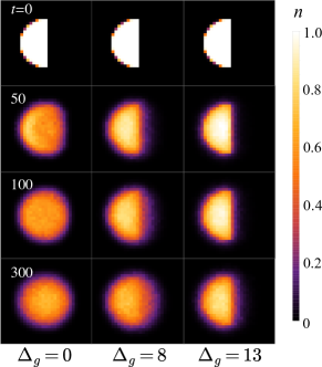
Figure 1: The site occupations for quenched dynamics at zero temperature. Columns (rows) depict results for different disorder strengths (different times). At time $t=0$ all bosons in the right half of the system are removed and the remainder evolves for $t>0$. The $t=0$ state is the ground state for a very small hopping and no disorder. For $t>0$, Gaussian disorder of strength $\Delta_{g}$ is introduced and the hopping is increased. The state evolves for $t\geq 0$ with no parameter changes.

Within GMFT, dynamics occur only when there are nonvanishing values of the order parameter $\phi_{{\bf{i}}}$ [see Eq. (3)]. As a result, a pure MI state would exhibit no dynamics within GMFT. We find that, as in Refs. Jreissaty et al. (2011); Yan et al. (2016), the small region with a non-vanishing order parameter generated by the harmonic trap at the edge of MI domains is sufficient to drive dynamics. Remarkably, we will see that the ensuing dynamics measured by imbalance is slower but similar to that in the experiments Choi et al. (2016) at long times. We will then show that decreasing $l_{x}$ to phenomenologically remove particles in the MI state significantly improves agreement with experiment.

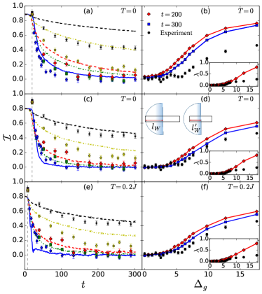
Figure 2: (a): Time evolution of the imbalance ${\cal I}$ for various disorder strengths at initial temperature $T=0$. Lines show simulation results while points with error bars show experimental data Choi et al. (2016). The vertical dashed line marks a time $t^{*}=20$ below which ${\cal I}$ barely changes within GMFT. The experimental results are shifted to start at $t^{*}$. From bottom to top the lines and symbols correspond to $\Delta_{g}=0,3,4,8,$ and $13$. (b): Corresponding ${\cal I}$ for the same parameters but at times $t=200$ and $300$ against disorder strength. The experimental result after an evolution time of $187$ are also plotted. The inset shows the inverse decay length [Eq. (5)] from our calculation at $t=200$ and for the experiment after an evolution time $t=187$. (c) and (d): The same as (a) and (b) but with an analysis window resized from $l_{W}=9$ [as in (a) and (b) following Ref. Choi et al. (2016)] to $l_{W}^{\prime}=5$, as shown in the schematic. (e) and (f): The same as (c) and (d) but at non-zero temperature. Here $t^{*}$ reduces to 8.

Qenched dynamics.— In the experiment Choi et al. (2016) the dynamics took place after lowering the lattice depth and introducing a disorder potential to a MI created in a deep lattice and to which all atoms in one half of the system were removed. From now on, we use the hopping parameter after the quench $J=U/24.4$ as our energy unit. To create the initial state, we used the experimental parameters Choi et al. (2016): $J_{I}=0.244$, $U=24.4$, $\Omega=0.145$, and $\mu=10.6$. After free energy minimization, particles on the right half of the system are manually removed [by setting $\alpha_{m,n}^{(i_{x}>0)}=\delta_{m,0}\delta_{n,0}$ in Eq. (2)], leaving behind a particle number comparable with the experiment, $N_{b}\approx 123$. In accordance with the experimental protocol Choi et al. (2016), to generate disorder (at the evolution stage) we square a two-dimensional array of uniformly distributed random numbers followed by a convolution with a Gaussian profile of standard deviation $0.5$. The disorder strength $\Delta_{g}$ is defined as the full width at half maximum of the resulting disorder profile.

The first column in Fig. 1 depicts the evolution of the site occupations in the absence of disorder. Here the particles expand to reach a steady state with no imbalance. When disorder of strength $\Delta_{g}=8$ is introduced, the motion slows considerably and an imbalance remains at the latest time shown. For very strong disorder ($\Delta_{g}=13$), the particles remain almost entirely in the initially occupied region.

To quantitatively understand the dynamics, we plot the imbalance against time in Fig. 2(a). For $t<t^{*}$, the imbalance barely changes. This is an artifact of GMFT for the initial state, which is mostly a MI domain. Beyond $t^{*}$, ${\cal I}$ vanishes rapidly in the clean limit and for weak disorder. But, as the disorder strength increases, it takes longer for ${\cal I}$ to reach the expected ${\cal I}=0$ steady state value. In Fig. 2(a), we also plot the experimental results taking $t^{*}$ to be the starting time for the experiments. The GMFT and experimental results exhibit good agreement for weak disorder strength, but the latter exhibit faster relaxation as the disorder strength is increased.

In Fig. 2(b), we plot the imbalance alongside experimental results Choi et al. (2016), as a function of the disorder strength. In our theoretical results, the upturn in ${\cal I}$ versus $\Delta_{g}$ moves toward stronger disorder strengths as $t$ increases. A similar trend was seen in experiments for $t\lesssim 200$, but the experimental results appeared to saturate for $200\lesssim t\lesssim 300$. For any given selected time, the upturn in ${\cal I}$ versus $\Delta_{g}$ occurs at a smaller value of $\Delta_{g}$ in GMFT when compared to the experiments, which is expected given the slower dynamics of the former seen in Fig. 2(a).

$\lambda$ offers another way to quantify the degree of localization by parameterizing the extent to which disorder suppresses the relaxation of site occupations. The inset in Fig. 2(b) shows $\lambda$ versus $\Delta_{g}$ for $t=200$ and the experimental results for $t=187$. The behavior of $\lambda$ (inset) is similar to that of ${\cal I}$ (main panel).

There are also differences between GMFT and experiments. For example, at weak disorder strengths, the experimental data of Fig. 2(b) exhibits oscillations not captured by GMFT. These oscillations in turn impact the comparison of the nature of upturns of ${\cal I}$ or $\lambda$ near $\Delta_{g}=5.5$, as they make it look sharper in the experimental results.

A key observable in identifying localization is the time derivative of the imbalance, $\dot{{\cal I}}$, at long times, as used in observations of Anderson localization with ultracold atoms Billy et al. (2008); Roati et al. (2008); Chabé et al. (2008); Lemarié et al. (2009); Kondov et al. (2011); Jendrzejewski et al. (2012). The vanishing of $\dot{{\cal I}}$ at long times (and in large system sizes) is a necessary condition for localization. The slope of ${\cal I}$ versus $t$ obtained for the four latest experimental times reported is $-1.017(\pm 1.028)\times 10^{-4}$ for the largest disorder strength. Here we see that the experimental error is too large to definitively show a vanishing of the slope since the results are also consistent with just a small slope. Within GMFT, we find a small non-zero slope: $-4.433(\pm 0.053)\times 10^{-4}$, for the largest disorder strength. The small non-zero slope shows that a slow rebalancing (as expected in the glassy state captured within GMFT) is consistent with experiment.

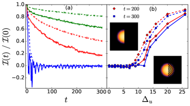
Figure 3: The solid (dashed) lines plot the normalized imbalance where the right half of the trap was initialized to a checkerboard (empty) pattern as shown in the insets. (a) The normalized imbalance against time for various disorder strengths. The pairs of (solid/dashed) lines correspond to uniform disorder $\Delta_{u}=0,13$ and $20$ from bottom to top. (b) The normalized imbalance at times $t=200$ and $300$ against disorder strength. The other parameters are $U=24.4$, $\Omega=0.145$, and $\mu=4$.

To understand the robustness of our findings within GMFT, we have also studied initial states at finite temperatures, different quench protocols, and dynamics in the presence of a uniform disorder distribution. The appendix shows that the latter two changes do not have much impact on the imbalance dynamics at long times. GMFT shows that the imbalance dynamics of a BG or MI quenched into a disorder profile respond in nearly the same way.

Phenomenological parameter.—To improve the comparison with the experiments we introduce a phenomenological parameter that excludes particles which move too slowly within GMFT. GMFT underestimates the speed of the MI dynamics under an applied field. The motion of the entire trapped system is therefore slower in GMFT at long times.

To account for the slow Mott particles we introduce a phenomenological parameter to our GMFT analysis. The inset of Fig. 2(d) shows a schematic of a resizing of the window used to compute the imbalance. The rectangles in the schematics indicate a decrease in $l_{x}$ in Eq. 4, from $l_{W}$ to $l_{W}^{\prime}$. Our phenomenological parameter, $l_{x}$, therefore increases the relative rate of rebalancing because slow moving Mott particles near the left edge of the system are excluded from the data analysis. Decreasing $\mu$ also removes these particles. We find that tuning either $\mu$ or $l_{x}$ allows us to fit ${\cal I}$ versus $t$ to experimental values with the same accuracy. We choose $l_{x}$ as our phenomenological parameter and vary it to obtain a best fit for the largest disorder, $\Delta_{g}=13$.

Figures 2(c) and 2(d) plot the same as panels (a) and (b) but with the new window size, $l_{W}^{\prime}$. Here there is much better agreement with experiment because the relative fraction of mobile to localized particles in our GMFT is closer to the experiment. Panels (e) and (f) include nonzero temperature. In varying $T$ we find little change for $T<J$. $T=0.2J$ was chosen as a best fit for the largest disorder. In Fig. 2(e) we see that $t^{*}$ diminishes and the imbalance tends to level off quicker at long times, with a slight increase in the slope to $-4.816(\pm 0.160)\times 10^{-4}$.

The comparisons between theory and experiment in Fig. 2 show that by adjusting a single phenomenological parameter we can bring GMFT into better agreement with experiments. We therefore conclude that the long-time relaxation found in experiments can be interpreted within GMFT as glassy dynamics consistent with the out of equilibrium properties of a BG and its excitations.

Checkerboard case.—The initial expansion of bosons in the empty half of the trap in the presence of disorder is expected to be dominated by Anderson physics, due to the low site occupations. In order to test how enhancing interactions by increasing site occupations affects the expansion, we have devised an “improved” initial state generated by emptying sites in one half of the system according to a checkerboard pattern. The dynamics then proceeds by allowing the remaining bosons to evolve without any change in the Hamiltonian parameters (no parameter quenching). Before emptying sites, the system was in the ground state.

Fig. 3 plots the normalized imbalance for the checkerboard pattern. The pattern speeds up the decay of ${\cal I}(t)/{\cal I}(0)$ by enhancing the effect of interactions during the dynamics. It would be interesting to find out how changes in the pattern used for the initial state change the results in the experiments Choi et al. (2016).

Discussion.—Motivated by Ref. Choi et al. (2016), we have studied the dynamics of bosons in 2D lattices with disorder by GMFT. We showed that theory becomes closer to experiment by including temperature and a single phenomenological parameter. We also showed that the features observed in the experiments are robust for various initial states: quenched MI, disordered superfluid, and BG. Since GMFT misses the entanglement present in MBL phases, evidence for MBL must lie in the differences between GMFT and experiments. We find that at the present stage with only the data from Ref. Choi et al. (2016), it is difficult to tell if there is a qualitative or quantitative difference between GMFT and experiments. Further experiments, particularly at longer times, will be needed to unambiguously show that MBL is occurring. Avoiding macroscopic mass transport, as done in Ref. Schreiber et al. (2015), will help rule out slow dynamics due to Anderson and BG physics.

Appendix: Non-quenched dynamics for uniformly distributed disorder

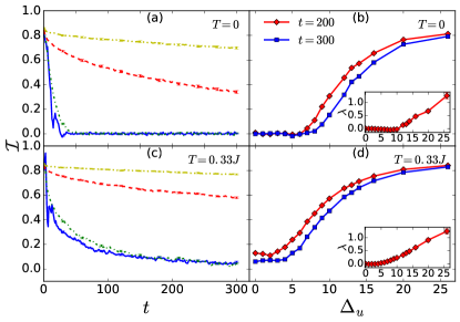
Figure 4: Time evolution of the imbalance ${\cal I}$ for various uniformly distributed disorder strengths when the initial temperature is $T=0$ (a) and $T=0.33$ (c). (b) and (d): Corresponding ${\cal I}$ for the same parameters but at times $t=200$ and $300$ against disorder strength. The initial state is the ground state of Eq.(1) of the main text for $U=24.4$, $\Omega=0.145$, and $\mu=4$ in the presence of uniformly distributed disorder with strength $\Delta_{u}$. In panels (a) and (c), the lines correspond to $\Delta_{u}=0,4,13$ and $20$ from bottom to top.

We test whether the quench protocol impacts the dynamics qualitatively. We consider a non-quenched parameter set and study the dynamics of the imbalance. We allow the ground state to settle into the disorder profile before time evolving the system. The initial state is not a Mott insulator but rather a SF (or a BG for large disorder disorder). Here we consider the dynamics after removing all bosons in one half of the system but without quenching any Hamiltonian parameters. For this protocol, the initial state is selected to be the ground state for the same values of $J$, $\Omega$, and $U$ as in the experiment after the quench, but we trap a smaller number of bosons (the site occupations in the center of the trap are still very close to those in the Mott insulating state). Different from the quenched dynamics, here we take the disorder to be distributed uniformly in the interval $[-\Delta_{u}/2,\Delta_{u}/2]$, to show that the qualitative results do not depend on the details of the disorder profile.

Figure 4(a) shows the time evolution of ${\cal I}$. Comparing Fig. 2(a) of the main text and Fig. 4(a) here one can see that the behavior of the non-quenched and quenched cases is qualitatively similar. Quantitative differences are, on the other hand, apparent. In the non-quenched dynamics there is no $t^{*}$ such that ${\cal I}$ does not change appreciably for $t<t^{*}$. This is because the order parameter in the non-Mott regime is sizable. In addition, ${\cal I}$ decays more quickly in the non-quenched than in the quenched case. This is expected for weak disorder strengths, for which the initial state is SF, but it is also the case in the BG regime present for strong disorder. The results for ${\cal I}$ against $\Delta_{u}$ [Fig. 4(b)] and for $\lambda$ against $\Delta_{u}$ [inset in Fig. 4(b)] are also qualitatively similar to the corresponding graphs in Fig. 2 of the main text. The onset of the localized regime increases as $t$ increases. Figs. 4(c) and 4(d) show that the dynamics of the system slows down with the introduction of a nonzero temperature in the initial state. This is understandable as nonzero temperatures reduce the magnitude of the order parameter in the SF and BG phases Buonsante et al. (2007). Overall, we find no qualitative change in comparing the quenched and non-quenched cases.

References

- Verkerk et al. (1992) P. Verkerk, B. Lounis, C. Salomon, C. Cohen-Tannoudji, J.-Y. Courtois, and G. Grynberg, Phys. Rev. Lett. 68, 3861 (1992).
- Jessen et al. (1992) P. S. Jessen, C. Gerz, P. D. Lett, W. D. Phillips, S. L. Rolston, R. J. C. Spreeuw, and C. I. Westbrook, Phys. Rev. Lett. 69, 49 (1992).
- Hemmerich and Hansch (1993) A. Hemmerich and T. W. Hansch, Phys. Rev. Lett. 70, 410 (1993).
- Bloch et al. (2008) I. Bloch, J. Dalibard, and W. Zwerger, Rev. Mod. Phys. 80, 885 (2008).
- Cazalilla et al. (2011) M. A. Cazalilla, R. Citro, T. Giamarchi, E. Orignac, and M. Rigol, Rev. Mod. Phys. 83, 1405 (2011).
- Köhl et al. (2005) M. Köhl, H. Moritz, T. Stöferle, K. Günter, and T. Esslinger, Phys. Rev. Lett. 94, 080403 (2005).
- Billy et al. (2008) J. Billy, V. Josse, Z. Zuo, A. Bernard, B. Hambrecht, P. Lugan, D. Clément, L. Sanchez-Palencia, P. Bouyer, and A. Aspect, Nature 453, 891 (2008).
- Roati et al. (2008) G. Roati, C. D’Errico, L. Fallani, M. Fattori, C. Fort, M. Zaccanti, G. Modugno, M. Modugno, and M. Inguscio, Nature 453, 895 (2008).
- Chabé et al. (2008) J. Chabé, G. Lemarié, B. Grémaud, D. Delande, P. Szriftgiser, and J. C. Garreau, Phys. Rev. Lett. 101, 255702 (2008).
- Lemarié et al. (2009) G. Lemarié, J. Chabé, P. Szriftgiser, J. Garreau, B. Grémaud, and D. Delande, Phys. Rev. A 80, 043626 (2009).
- Kondov et al. (2011) S. S. Kondov, W. R. McGehee, J. J. Zirbel, and B. DeMarco, Science 334, 66 (2011).
- Jendrzejewski et al. (2012) F. Jendrzejewski, A. Bernard, K. Mulller, P. Cheinet, V. Josse, M. Piraud, L. Pezze, L. Sanchez-Palencia, A. Aspect, and P. Bouyer, Nat. Phys. 8, 398 (2012).
- Greiner et al. (2002) M. Greiner, O. Mandel, T. Esslinger, T. W. Hansch, and I. Bloch, Nature 415, 39 (2002).
- Stöferle et al. (2004) T. Stöferle, H. Moritz, C. Schori, M. Köhl, and T. Esslinger, Phys. Rev. Lett. 92, 130403 (2004).
- Spielman et al. (2007) I. B. Spielman, W. D. Phillips, and J. V. Porto, Phys. Rev. Lett. 98, 080404 (2007).
- Jordens et al. (2008) R. Jordens, N. Strohmaier, K. Guenther, H. Moritz, and T. Esslinger, Nature 455, 204 (2008).
- Schneider et al. (2008) U. Schneider, L. Hackermueller, S. Will, T. Best, I. Bloch, T. A. Costi, R. W. Helmes, D. Rasch, and A. Rosch, Science 322, 1520 (2008).
- Chen et al. (2008) Y. P. Chen, J. Hitchcock, D. Dries, M. Junker, C. Welford, and R. G. Hulet, Phys. Rev. A 77, 033632 (2008).
- White et al. (2009) M. White, M. Pasienski, D. McKay, S. Q. Zhou, D. Ceperley, and B. DeMarco, Phys. Rev. Lett. 102, 055301 (2009).
- Pasienski et al. (2010) M. Pasienski, D. McKay, M. White, and B. DeMarco, Nat. Phys. 6, 677 (2010).
- Gadway et al. (2011) B. Gadway, D. Pertot, J. Reeves, M. Vogt, and D. Schneble, Phys. Rev. Lett. 107, 145306 (2011).
- Beeler et al. (2012) M. C. Beeler, M. E. W. Reed, T. Hong, and S. L. Rolston, New J. Phys. 14, 073024 (2012).
- Brantut et al. (2012) J.-P. Brantut, J. Meineke, D. Stadler, S. Krinner, and T. Esslinger, Science 337, 1069 (2012).
- Tanzi et al. (2013) L. Tanzi, E. Lucioni, S. Chaudhuri, L. Gori, A. Kumar, C. D’Errico, M. Inguscio, and G. Modugno, Phys. Rev. Lett. 111, 115301 (2013).
- Krinner et al. (2013) S. Krinner, D. Stadler, J. Meineke, J. P. Brantut, and T. Esslinger, Phys. Rev. Lett. 110, 100601 (2013).
- Kondov et al. (2015) S. S. Kondov, W. R. McGehee, W. Xu, and B. DeMarco, Phys. Rev. Lett. 114, 083002 (2015).
- Schreiber et al. (2015) M. Schreiber, S. S. Hodgman, P. Bordia, H. P. Lüschen, M. H. Fischer, R. Vosk, E. Altman, U. Schneider, and I. Bloch, Science 349, 842 (2015).
- Choi et al. (2016) J.-Y. Choi, S. Hild, J. Zeiher, P. Schaub, A. Rubio-Abadal, T. Yefsah, V. Khemani, D. A. Huse, I. Bloch, and C. Gross, (2016), arXiv:1604.04178 .
- Fisher et al. (1989) M. P. A. Fisher, P. B. Weichman, G. Grinstein, and D. S. Fisher, Phys. Rev. B 40, 546 (1989).
- Scalettar et al. (1991) R. T. Scalettar, G. G. Batrouni, and G. T. Zimanyi, Phys. Rev. Lett. 66, 3144 (1991).
- Basko et al. (2006) D. M. Basko, I. L. Aleiner, and B. L. Altshuler, Ann. Phys. 321, 1126 (2006).
- Oganesyan and Huse (2007) V. Oganesyan and D. A. Huse, Phys. Rev. B 75, 155111 (2007).
- Pal and Huse (2010) A. Pal and D. Huse, Phys. Rev. B 82, 174411 (2010).
- Deutsch (1991) J. M. Deutsch, Phys. Rev. A 43, 2046 (1991).
- Srednicki (1994) M. Srednicki, Phys. Rev. E 50, 888 (1994).
- Rigol et al. (2008) M. Rigol, V. Dunjko, and M. Olshanii, Nature 452, 854 (2008).
- Nandkishore and Huse (2015) R. Nandkishore and D. A. Huse, Annu. Rev. Condens. Matter Phys. 6, 15 (2015).
- Scarola and DeMarco (2015) V. W. Scarola and B. DeMarco, Phys. Rev. A 92, 053628 (2015).
- Mondaini and Rigol (2015) R. Mondaini and M. Rigol, Phys. Rev. A 92, 041601 (2015).
- Rokhsar and Kotliar (1991) D. S. Rokhsar and B. G. Kotliar, Phys. Rev. B 44, 10328 (1991).
- Jaksch et al. (1998) D. Jaksch, C. Bruder, J. I. Cirac, C. W. Gardiner, and P. Zoller, Phys. Rev. Lett. 81, 3108 (1998).
- Hen and Rigol (2009) I. Hen and M. Rigol, Phys. Rev. B 80, 134508 (2009).
- Hen et al. (2010) I. Hen, M. Iskin, and M. Rigol, Phys. Rev. B 81, 064503 (2010).
- Sheshadri et al. (1995) K. Sheshadri, H. R. Krishnamurthy, R. Pandit, and T. V. Ramakrishnan, Phys. Rev. Lett. 75, 4075 (1995).
- Damski et al. (2003) B. Damski, J. Zakrzewski, L. Santos, P. Zoller, and M. Lewenstein, Phys. Rev. Lett. 91, 080403 (2003).
- Buonsante et al. (2007) P. Buonsante, V. Penna, A. Vezzani, and P. B. Blakie, Phys. Rev. A 76, 011602 (2007).
- Buonsante et al. (2009) P. Buonsante, F. Massel, V. Penna, and A. Vezzani, Phys. Rev. A 79, 013623 (2009).
- Lin et al. (2012) C. H. Lin, R. Sensarma, K. Sengupta, and S. Das Sarma, Phys. Rev. B 86, 214207 (2012).
- Jaksch et al. (2002) D. Jaksch, V. Venturi, J. I. Cirac, C. J. Williams, and P. Zoller, Phys. Rev. Lett. 89, 040402 (2002).
- Zakrzewski (2005) J. Zakrzewski, Phys. Rev. A 71, 043601 (2005).
- Snoek and Hofstetter (2007) M. Snoek and W. Hofstetter, Phys. Rev. A 76, 051603 (2007).
- Wolf et al. (2010) F. A. Wolf, I. Hen, and M. Rigol, Phys. Rev. A 82, 043601 (2010).
- Snoek (2011) M. Snoek, Europhys. Lett. 95, 30006 (2011).
- Hen and Rigol (2010) I. Hen and M. Rigol, Phys. Rev. A 82, 043634 (2010).
- Jreissaty et al. (2011) M. Jreissaty, J. Carrasquilla, F. A. Wolf, and M. Rigol, Phys. Rev. A 84, 043610 (2011).
- Yan et al. (2016) M. Yan, H.-Y. Hui, and V. W. Scarola, (2016), arXiv:1601.06817 .
- Bauer and Nayak (2013) B. Bauer and C. Nayak, J. Stat. Mech: Theory Exp. 2013, P09005 (2013).
- Kim and Huse (2013) H. Kim and D. A. Huse, Phys. Rev. Lett. 111, 127205 (2013).
- Bardarson et al. (2012) J. H. Bardarson, F. Pollmann, and J. E. Moore, Phys. Rev. Lett. 109, 017202 (2012).