Guaranteed Cost Approach for Robust Model Predictive Control of Uncertain Linear Systems

Abstract

In this paper we propose a constrained guaranteed cost robust model predictive controller (GCMPC) for uncertain discrete time systems. This controller was developed based on a quadratic cost functional and guarantee robustness with respect to quadratically bound uncertainties. Such a class of problems is currently intractable by Min-Max Robust Model Predictive Controllers without polytopic approximations of the uncertainties. The proposed technique is computationally more efficient then an enumeration-based approach and requires only a Quadratically Constrained Quadratic Problem (QCQP) optimization, whereas LMI-based GCMPC approaches require a Semi-Definite Programming (SDP) optimization.

I INTRODUCTION

Model Predictive Control (MPC) is a class of optimization-based control algorithms that uses an explicit model of the controlled system to predict its future states [3]. The technique has been used in several different areas, such as refineries, food processing plants, mining, aerospace and automotive control [20]. MPC objective is to minimize a cost functional and maintain the system states and control inputs within a feasible set. The system dynamics are usually assumed to be known. Therefore, model mismatches or external disturbances are not considered. However, the disregard of such uncertainties may lead to poor closed-loop performance and the violation of state and control input constraints [22].

Robust Model Predictive Control (RMPC) addresses the poor closed-loop performance subject to uncertainties [5]. The main RMPC approach is based on Min-Max optimization. Its objective is to obtain a control input sequence that minimizes a cost functional and to guarantee the feasibility of system states and control inputs when the system is subject to the worst-case disturbance. Most Min-Max Model Predictive Controllers (MMMPC) are based on different assumptions and approximations, therefore comparisons among different approaches are difficult. However, most of them are classified into two categories [14], namely open-loop and feedback MMMPC. The open-loop MMMPC is similar to the nominal MPC, in which a control input sequence is optimized with respect to the open-loop system. It is considered conservative for actual applications. On the other hand, feedback MMMPC optimizes a control input sequence with respect to a disturbance-rejecting closed-loop system, which addresses the conservativeness of the open-loop approach.

MMMPC schemes are defined by exact or approximate solutions to $l1$-norm, $l2$-norm or $l\infty$-norm cost functionals subject to polytopic bounded uncertainties (e.g. bound by $l1$-norm or $l\infty$-norm) [15, 24, 9]. Both $l1$-norm and $l\infty$-norm MMMPC problems may be approximated by Linear Programming (LP) problems without significant increase in the optimization problem complexity. However, $l2$-norm MMMPCs can be represented only by explicit enumeration of all vertexes of the uncertainty polytopic set [8, 4]. The enumeration approach suffers from Bellman’s curse of dimensionality, since the number of vertexes grows exponentially with the number of dimensions. This issue is further aggravated if the uncertainty set is defined by $l2$-norm, as the enumeration approach cannot be performed on non-polytopic sets.

Xie and Soh [26] designed the Guaranteed Cost Control (GCC) to address the poor performance of the Linear Quadratic Regulator (LQR) when a Linear Time Invariant (LTI) system model is subject to $l2$-norm bounded parametric uncertainties. It provides a quadratically stable closed-form controller that guarantees an upper bound to $l2$-norm cost functionals. However, the GCC design considers only unconstrained control problem.

GCCs are obtained by either Linear Matrix Inequalities (LMI) [19] or Algebraic Riccati Equations (ARE) [26] and the concept was extended to polytopic-bounded $l2$-norm RMPCs problems based on LMIs [21, 23]. However, a semi-definite programming (SDP) problem must be solved for the guaranteed cost constrained optimization, which increases computational requirements in comparison to LPs, QPs and QCQPs.

In this paper we propose a Guaranteed Cost approach for Robust Model Predictive Control (GCMPC) of linear time invariant systems subject to bounded parametric uncertainties. This approach provides a QCQP-based solution to $l2$-norm Robust Model Predictive Controllers subject to $l2$-norm bounded uncertainties and polytopic constraints and ensures sufficient conditions for stability, feasibility and performance robustness.

This paper is organized as follows: Section II presents the robust constrained optimal control problem; Section III derives the Guaranteed Cost Model Predictive Controller; Section IV provides a numerical example; finally, Section V addresses the final remarks.

II PROBLEM STATEMENT AND PRELIMINARIES

This study investigates the formulation of the Guaranteed Cost Model Predictive Control (GCMPC) for linear systems subject to parametric uncertainties. A deterministic LTI system model (Definition 1) and a parametrically uncertain one (Definition 2) were considered for the formulation.

Definition 1

Let the discrete state space LTI model be

$$x_{k+1}=Fx_{k}+Gu_{k}$$ (1)

where $x_{k}\in\mathds{R}^{n}$ is the system state, $u_{k}\in\mathds{R}^{m}$ is the control input, $F\in\mathds{R}^{n\times n}$ is the state matrix and $G\in\mathds{R}^{n\times m}$ is the input matrix.

Definition 2

[25] Let the discrete state space LTI model subject to parametric uncertainties be

$$\bar{x}_{k+1}=(F+\delta F_{k})\bar{x}_{k}+(G+\delta G_{k})u_{k}$$ (2)

where $\bar{x}_{k}\in\mathds{R}^{n}$ is the uncertain system state and $\delta F_{k}$ and $\delta G_{k}$ are, respectively, the state and input multiplicative uncertainty matrices, such that

$$\begin{bmatrix}\delta F_{k}\;\delta G_{k}\end{bmatrix}=H\Delta_{k}\begin{bmatrix}E_{1}\;E_{2}\end{bmatrix}$$ (3)

with $\mathcal{W}=\{\delta\mid\delta\in\mathds{R}^{p\times l},||\delta||_{2}\leq 1\}$, $H\in\mathds{R}^{n\times p},H\neq 0$, $E_{1}\in\mathds{R}^{l\times n}$ and $E_{2}\in\mathds{R}^{l\times m}$.

Optimality is defined by a quadratic cost functional for LQR and $l2$-norm MPC approaches, given by

$$J_{i}(x_{i},\textbf{u},N)=x_{N}^{T}P_{n}x_{N}+\underset{k=i}{\overset{N-1}{\sum}}x_{k}^{T}Qx_{k}+u_{k}^{T}Ru_{k}$$ (4)

where $P_{N}\succeq 0$, $Q\succeq 0$ and $R\succ 0$ are symmetric weight matrices, $\mathbf{u}=\{u_{k}\mid k\in\mathds{Z}_{\geq 0}\cap[0,N-1]\}$ and the system model satisfies either Definition 1, or 2.

Definition 3

[13] Consider the deterministic system model from Definition 1. The Linear Quadratic Regulator is a feedback controller given by the optimal control problem

$$\begin{matrix}[l]J_{i}^{*}(x_{i},N)=&\underset{\mathbf{u}}{\inf}&J_{i}(x_{0},\mathbf{u},N)\\ &s.t.&x_{k+1}=Fx_{k}+Gu_{k}\end{matrix}$$ (5)

which has a closed form solution $J_{i}^{*}(x_{0})=x_{i}^{T}P_{i}x_{i}$ achieved at $u_{k}=-K_{k}x_{k}$, where

$$\begin{matrix}[l]K_{k}&=(R+G^{T}P_{k+1}G)^{-1}G^{T}P_{k+1}F\\ P_{k}&=F^{T}P_{k+1}F+Q-K_{k}^{T}(R+G^{T}P_{k+1}G)K_{k}\\ \end{matrix}$$ (6)

Definition 4

[7] Consider the deterministic system model from Definition 1. A Model Predictive Control is a feedback controller given by the constrained optimal control problem

$$\begin{matrix}[l]J_{i}^{*}(x_{i},N)=&\underset{\mathbf{u}}{\inf}&J_{i}(x_{0},\mathbf{u},N)\\ &s.t.&x_{k+1}=Fx_{k}+Gu_{k}\\ &&[x_{k}^{T},u_{k}^{T}]^{T}\in\mathcal{C}_{k}\end{matrix}$$ (7)

where $\mathcal{C}_{k}$ defines the feasible set of the system states and control inputs at timestep $k$.

MPC has no general closed form solution. Therefore, it requires either an online evaluation with a Quadratic Programming solver [16], or an offline evaluation based on explicit solutions [1].

Assumption 1

The feasible set of variables $x_{k}$ and $u_{k}$ at a given timestep $k$, given by $\left[x_{k}^{T},u_{k}^{T}\right]^{T}\in\mathcal{C}_{k}$, is a convex non-empty polytope described by

$$\mathcal{C}_{k}=\left\{z\mid z\in\mathds{R}^{n+m},C_{k}z+c_{k}\leq 0\right\}$$ (8)

where $C_{k}=[A_{k},B_{k}]$ with $A_{k}\in\mathds{R}^{q\times n}$ and $B_{k}\in\mathds{R}^{q\times m}$

Assumption 1 enables the use of widely available QP solvers (e.g. Gurobi [11], CVXGEN [18] and FORCES Pro [10]) and the solution of several practical control problems. Therefore, it is used in most MPC applications. However, neither LQR, nor MPC provides performance, stability or feasibility robustness guarantees when they are used for the control of systems subject to multiplicative or additive uncertainties.

Definition 5

[19] Consider the system model from Definition 2. A control law $u_{k}=-K_{k}\bar{x}_{k}$ is said to be a Guaranteed Cost Controller if there exists a symmetric cost matrix sequence $\mathcal{S}=\{S_{k}\mid S_{k}\succeq 0,k\in\mathds{Z},k\in[0,N]\}$, such that

$$\left[F-GK_{k}+\delta F_{k}-\delta G_{k}K_{k}\right]^{T}S_{k+1}\left[\bullet\right]-\\ -S_{k}+Q+K_{k}^{T}RK_{k}<0$$ (9)

where $z^{T}M(\bullet)=z^{T}Mz$.

By definition, GCC ensures the quadratic stability of the system for any disturbance within the admissible set $\mathcal{W}$. A closed form solution for $\mathcal{S}$ based on AREs is proposed by Xie and Soh [26].

Theorem 1

Consider the parametrically uncertain system model from Definition 2 and assume a control law $u_{k}=-K_{k}\bar{x}_{k}$ is a Guaranteed Cost Control with an associated cost matrix $S_{k}$. For some $\epsilon_{k}>0$, such that $S_{k}\succ 0$, the closed loop uncertain system

$$\bar{x}_{k+1}=[F-GK_{k}+\delta F_{k}-\delta G_{k}K_{k}]\bar{x}_{k}$$ (10)

has an upper bound cost

$$J_{k}(\bar{x}_{k},\mathbf{u},N)<\bar{x}_{k}^{T}S_{k}\bar{x}_{k}$$ (11)

given by

$$S_{k}=F^{T}X_{k+1}F+Q+\epsilon_{k}^{-1}E_{1}^{T}E_{1}-\\ -(F^{T}X_{k+1}G+\epsilon_{k}^{-1}E_{1}^{T}E_{2})(R+\epsilon_{k}^{-1}E_{2}^{T}E_{2}+G^{T}X_{k+1}G)^{-1}(\bullet)$$ (12)

where $I-\epsilon_{k}H^{T}S_{k}H\succ 0$ and

$$X_{k}= \left(S_{k}^{-1}-\epsilon_{k}^{-1}HH^{T}\right)^{-1}\succ 0$$ (13)

$$K_{k}= (R_{\epsilon k}+G^{T}X_{k+1}G)^{-1}(G^{T}X_{k+1}F+\epsilon_{k}^{-1}E_{2}^{T}E_{1}).$$ (14)

Proof:

See [26]. ∎

However, the results from Theorem 1 are valid only for $[\bar{x}_{k}^{T},u_{k}^{T}]^{T}\in\mathds{R}^{n+m}$ and have not been extended to the constrained quadratic optimal control case.

III GUARANTEED COST MODEL PREDICTIVE CONTROL

This section addresses the formulation of the constrained guaranteed cost control.

Lemma 1

Let $\epsilon\in\left(0,||H^{T}SH||\right)$ and

$$X=\left(S^{-1}-\epsilon HH^{T}\right)^{-1}\succ 0$$ (15)

for a given symmetric $S\succ 0$ and a non-singular $H$. Then, $X\succ S$.

Proof:

We employ Woodbury’s matrix inversion Lemma [12] to (15), which results in

$$X=S+SH\left(\epsilon^{-1}I-H^{T}SH\right)^{-1}H^{T}S$$ (16)

and conclude, from $\epsilon^{-1}I-H^{T}SH\succ 0$,

$$SH\left(\epsilon^{-1}I-H^{T}SH\right)^{-1}H^{T}S\succ 0$$ (17)

Therefore, $X\succ S$. ∎

Theorem 2

Consider the deterministic system model from Definition 1 and

$$\begin{matrix}[l]\bar{J}_{i}^{*}(x_{i},N)=&\underset{\mathbf{u}}{\inf}&\bar{J}_{i}(x_{i},\mathbf{u},N)\\ &s.t.&x_{k+1}=Fx_{k}+Gu_{k}\end{matrix}$$ (18)

where

$$\bar{J}_{i}(x_{i},\mathbf{u},N) =x_{N}^{T}S_{N}x_{N}+\underset{k=i}{\overset{N}{\sum}}c(x_{k},u_{k})$$ (19)

$$c(x,u) =x^{T}Q_{\epsilon k}x+u^{T}R_{\epsilon_{k}}u+2x^{T}N_{\epsilon_{k}}u$$ (20)

with $Q_{\epsilon k}=Q+\epsilon^{-1}E_{1}^{T}E_{1}$, $R_{\epsilon k}=R+\epsilon^{-1}E_{2}^{T}E_{2}$, $N_{\epsilon k}=\epsilon^{-1}E_{1}^{T}E_{2}$ and $\epsilon$ is chosen such that the guaranteed cost control condition is satisfied. The guaranteed cost control is equivalent to the sub-optimal solution of (18), given by

$$\begin{matrix}[l]\bar{J}_{N}(x_{N})&<x_{N}^{T}X_{N}x_{N}\\ \bar{J}_{k}(x_{k})&<\underset{u_{k}}{\inf}\;c(x_{k},u_{k})+x_{k+1}^{T}X_{k+1}x_{k+1}=x_{k}^{T}S_{k}x_{k}\end{matrix}$$ (21)

Proof:

Let the value function $\bar{J}^{*}_{k}(x)$, related to the optimization problem from (18), be recursively defined as

$$\bar{J}^{*}_{N}(x) =x^{T}S_{N}x$$ (22)

$$\bar{J}^{*}_{k}(x) =\underset{u}{\inf}\;c(x,u)+\bar{J}_{k+1}(Fx+Gu)$$ (23)

based on Bellman’s optimality principle.

From Lemma 1 and (22),

$$\bar{J}^{*}_{N}(x)=x^{T}S_{N}x<x^{T}X_{N}x$$ (24)

Therefore,

$$\bar{J}^{*}_{N-1}(x) =\underset{u}{\inf}\;c(x,u)+(Fx+Gu)^{T}S_{N}(\bullet)$$ (25)

$$<\underset{u}{\inf}\;c(x,u)+(Fx+Gu)^{T}X_{N}(\bullet)$$ (26)

The solution of (26) yields

$$u=-(R_{\epsilon_{k}}+G^{T}X_{N}G)^{-1}(G^{T}X_{N}F+N_{\epsilon_{k}})x$$ (27)

which substituted back in (26) results in

$$\bar{J}^{*}_{N-1}(x)<x^{T}\left[F^{T}X_{N}F+Q_{\epsilon k}-\right.\\ \left.-(F^{T}X_{N}G+N_{\epsilon k})(R_{\epsilon k}+G^{T}X_{N}G)^{-1}(\bullet)\right]x$$ (28)

Therefore, $\bar{J}^{*}_{N-1}(x)<x^{T}S_{N-1}x$, where $S_{N-1}$ is the guaranteed cost matrix at timestep $k=N-1$, as stated in Theorem 1.

Assume $\exists k\in\mathds{Z}_{\geq 0}\cap[0,N-2]:\;\bar{J}^{*}_{k+1}(x)<x^{T}S_{k+1}x$, where $S_{k+1}$ is a guaranteed cost matrix.

$$\bar{J}^{*}_{k}(x) <\underset{u}{\inf}\;c(x,u)+(Fx+Gu)^{T}S_{k+1}(\bullet)$$ (29)

$$<\underset{u}{\inf}\;c(x,u)+(Fx+Gu)^{T}X_{k+1}(\bullet)$$ (30)

which, analogously to $\bar{J}_{N-1}$, results in

$$\bar{J}_{k}(x)<x^{T}\left[F^{T}X_{k+1}F+Q_{\epsilon k}-\right.\\ \left.-(F^{T}X_{k+1}G+N_{\epsilon k})(R_{\epsilon k}+G^{T}X_{k+1}G)^{-1}(\bullet)\right]x$$ (31)

Therefore, we conclude by induction

$$\forall k\in\mathds{Z}_{\geq 0}\cap[0,N-1].\;\bar{J}_{k}(x)<x^{T}S_{k}x$$ (32)

hence the guaranteed cost control is a sub-optimal solution to the optimization problem in (18). ∎

Theorem 2 demonstrates the equivalence of the GCC of a parametrically uncertain system to a sub-optimal solution of a Dynamic Programming problem for the deterministic system model. It also shows that the GCC bounds $J_{i}^{*}(\bar{x}_{i},\mathbf{u},N)<x_{i}^{T}S_{i}x_{i}$ and $\bar{J}_{i}^{*}(x_{i},\mathbf{u},N)<x_{i}^{T}S_{i}x_{i}$. However, the result from Theorem 2 is valid only for the unconstrained case where $x_{k}\in\mathds{R}^{n}$ and $u_{k}\in\mathds{R}^{m}$.

Lemma 2

Consider the parametrically uncertain system model from Definition 2 and let $K_{k}$ be a guaranteed cost control, $u_{k}=-K_{k}\bar{x}_{k}+v_{k}$ and $\bar{R}_{k}=R_{\epsilon k}+G^{T}X_{k+1}G$.

$$\begin{matrix}[l]J_{i}^{*}(x_{i},\mathbf{u},N)<&\underset{\mathbf{v}}{\inf}&\underset{k=i}{\overset{N-1}{\sum}}v_{k}\bar{R}_{k}v_{k}+x_{i}^{T}S_{i}x_{i}\\ &s.t.&x_{k+1}=(F-GK_{k})x_{k}+Gv_{k}\\ \end{matrix}$$ (33)

is equivalent to the guaranteed cost control sub-optimal solution from Theorem 2.

Proof:

Consider the value function from (21) and the deterministic system model from Definition 1.

$$\bar{J}^{*}_{k}(x)<\underset{u}{\inf}\;x^{T}(Q_{\epsilon k}+F^{T}X_{k+1}F)x+\\ +u^{T}(R_{\epsilon k}+G^{T}X_{k+1}G)u+2x^{T}F^{T}X_{k+1}Gu$$ (34)

where the substitution of $u=K_{k}x_{k}+v_{k}$ yields

$$\bar{J}^{*}_{k}(x)<x^{T}S_{k}x+\underset{v}{\inf}\;v^{T}(R_{\epsilon k}+G^{T}X_{k+1}G)v$$ (35)

The recursive substitution of (35) for $k\in[i,N-1]$ results in

$$\begin{matrix}[l]\bar{J}^{*}_{i}(x_{i})<&\underset{\mathbf{v}}{\inf}&\underset{k=i}{\overset{N-1}{\sum}}v_{k}\bar{R}v_{i}+x_{i}^{T}S_{i}x_{i}\\ &s.t.&x_{k+1}=(F-GK_{k})x_{k}+Gv_{k}\\ \end{matrix}$$ (36)

Therefore, from the results of Theorem 2 and [26],

$$\begin{matrix}[l]J_{i}^{*}(x_{i},\mathbf{u},N)<&\underset{\mathbf{v}}{\inf}&\underset{k=i}{\overset{N-1}{\sum}}v_{k}\bar{R}v_{i}+x_{i}^{T}S_{i}x_{i}\\ &s.t.&x_{k+1}=(F-GK_{k})x_{k}+Gv_{k}\\ \end{matrix}$$ (37)

∎

If the optimization domain of (33) is $\mathcal{C}_{k}\equiv\mathds{R}^{n+m}$, the solution is trivially $v_{k}\equiv 0$ and (33) reduces to Theorem 2. However, if $\mathcal{C}_{k}\subset\mathds{R}^{n+m}$, (33) provides an upper bound to the MPC cost functional.

Since (37) is based on the deterministic model, enforcement of the feasible set constraints ($[x_{k}^{T},u_{k}^{T}]^{T}\in\mathcal{C}_{k}$) would ensure that only the undisturbed states and control inputs are feasible and there would be no feasibility guarantees for the parametrically uncertain ones. Feasibility robustness requires

$$\forall\Delta_{k}\in\mathcal{W}.\;[\bar{x}_{k}^{T},u_{k}^{T}]^{T}\in\mathcal{C}_{k}$$ (38)

Lemma 3

Consider the parametrically uncertain system model from Definition 2 and let $K_{k}$ be a Guaranteed Cost Controller, $u_{k}=-K_{k}\bar{x}_{k}+v_{k}$ and $\mathcal{\bar{W}}_{k}=\{w\mid w\in\mathds{R}^{p\times l},||w||_{2}\leq||\widetilde{E}_{1}\bar{x}_{k}+E_{2}v_{k}||_{2}\}$ where $\widetilde{E}_{1}=E_{1}-E_{2}K_{k}$.

$$\bar{x}_{k+1}=(F-GK_{k})\bar{x}_{k}+Gv_{k}+Hw_{k}$$ (39)

is an approximation of the closed loop parametrically uncertain model.

Proof:

Let $w_{k}=\Delta_{k}[\widetilde{E}_{1,k}\bar{x}_{k}+E_{2}v_{k}]$. From (39), we conclude

$$\begin{matrix}[l]\bar{x}_{k+1}&=(F-GK_{k})\bar{x}_{k}+Gv_{k}+H\Delta_{k}(\widetilde{E}_{1,k}\bar{x}_{k}+E_{2}v_{k})\\ &=F\bar{x}_{k}+Gu_{k}+H\Delta_{k}(E_{1}\bar{x}_{k}+E_{2}u_{k})\\ &=(F+\delta F_{k})\bar{x}_{k}+(G+\delta G_{k})u_{k}\end{matrix}$$ (40)

and the admissible set of $w_{k}$, $\mathcal{\bar{W}}$, is given by

$$\begin{matrix}[l]||w_{k}||_{2}&=||\Delta_{k}[\widetilde{E}_{1,k}\bar{x}_{k}+E_{2}v_{k}]||_{2}\\ &\leq||\Delta_{k}||_{2}||\widetilde{E}_{1,k}\bar{x}_{k}+E_{2}v_{k}||_{2}\\ &\leq||\widetilde{E}_{1,k}\bar{x}_{k}+E_{2}v_{k}||_{2}\end{matrix}$$ (41)

Therefore, $\mathcal{\bar{W}}_{k}=\{w\mid w\in\mathds{R}^{p\times l},||w||_{2}\leq||\widetilde{E}_{1}\bar{xs}_{k}+E_{2}v_{k}||_{2}\}$. Since $\mathcal{\bar{W}}\supset\mathcal{W}$, such a representation is a conservative approximation of Definition 2. ∎

Lemma 3 provides a conservative approximation to the parametrically uncertain system. Such representation enables multiplicative uncertainties to be modeled as in previous RMPC studies (i.e. [24]).

Corollary 1

Consider the deterministic and parametrically uncertain system models from Definition 1 and Lemma 3, respectively, and assume the system is regulated by a feedback controller $\widetilde{K}$.

$$\bar{x_{k}}=x_{k}+\underset{i=0}{\overset{k-1}{\sum}}\widetilde{F}^{k-i-1}Hw_{i}$$ (42)

where $\widetilde{F}=F-G\widetilde{K}$ is the closed loop system dynamics.

Corollary 1 provides a representation of the uncertain system state according to the deterministic system state and all previous disturbances and enables the externalization of disturbances from the system dynamics to the feasible set constraints. Therefore, based on (38) and Assumption 1, the parametrically uncertain model feasible set $\mathcal{C}_{k}$ with $u_{k}=-K_{k}x_{k}+v_{k}$ is

$$\forall w_{k}\in\mathcal{\bar{W}}.\;\widetilde{A}_{k}x_{k}+B_{k}v_{k}+c_{k}+\\ +\widetilde{A}_{k}\underset{i=0}{\overset{k-1}{\sum}}\widetilde{F}^{k-i-1}Hw_{i}\leq 0$$ (43)

where $\widetilde{A}_{k}=A_{k}-B_{k}K_{k}$ and $\widetilde{K}$ is arbitrarily defined. However, uncertainty admissible set $\mathcal{\bar{W}}$ is still dependent on uncertain state $\bar{x}_{k}$.

Lemma 4

Let $\phi_{k}(x,v)=||\widetilde{E}_{1,k}x+E_{2}v||_{2}$ and $\rho_{i}=||E_{1}\widetilde{F}^{i}H||_{2}$. Then,

$$||w_{k}||\leq\phi_{k}(\bar{x}_{k},v_{k})\leq\\ \phi_{k}(x_{k},v_{k})+\underset{i=0}{\overset{k-1}{\sum}}c(k,i)\phi_{i}(x_{i},v_{i})$$ (44)

where

$$\forall i<k.\;c(k,i)=\rho_{k-i-1}+\underset{j=0}{\overset{k-i-2}{\sum}}\rho_{j}c(k-j-1,i)$$ (45)

Proof:

Omitted. ∎

Duality filter, enumeration filter, explicit maximization filter, Pólya filter and elimination filter are five main approaches that devise robust counterparts of $\mathcal{C}_{k}$ [17], such that (38) is satisfied for an optimization based on the deterministic model. Pólya and elimination filters are relaxations of the constraints and are not sufficient conditions to satisfy (43). Enumeration and the duality filters cause the number of variables to grow significantly. Therefore, this study has focused on the explicit maximization filter.

Definition 6

Given an uncertain variable $w\in\{w\mid w\in\mathds{R}^{n},||w||_{p}\leq 1\}$ and an inequality constraint

$$(A^{T}w+b)^{T}x+(c^{T}w+d)\leq 0$$ (46)

The robust constraint counterpart by explicit maximization is given by

$$b^{T}x+d+||Ax+c||_{p^{*}}\leq 0$$ (47)

where $||z||_{p^{*}}$ is the dual norm [6] of $||Ax+c||_{p}$ and satisfies $1/p+1/p^{*}=1$.

Theorem 3

Let $\bar{\mathcal{C}}_{k}$ be the robust counterpart of $\mathcal{C}_{k}$ by explicit maximization and, based on Lemma 4, $\bar{\phi}_{k}(\mathbf{x},\mathbf{v})=\phi_{k}(x_{k},v_{k})+\underset{i=0}{\overset{k-1}{\sum}}c(k,i)\phi_{i}(x_{i},v_{i})$. Then,

$$\bar{\mathcal{C}}_{k}=\{[x_{k}^{T},v_{k}^{T}]^{T}\mid x_{k}\in\mathds{R}^{n},v_{k}\in\mathds{R}^{m},\forall i\in\mathds{I}\cap[1,q].\\ \widetilde{A}_{k}^{(i)}x_{k}+B_{k}^{(i)}v_{k}+c_{k}^{(i)}+\Phi_{k,i}(\mathbf{x},\mathbf{v})\leq 0\}$$ (48)

where $\Phi_{k,i}(\mathbf{x},\mathbf{v})=\underset{j=0}{\overset{k-1}{\sum}}||\widetilde{A}_{k}^{(i)}\widetilde{F}^{k-j-1}H||_{2}\bar{\phi}_{j}(\mathbf{x},\mathbf{v})$ and $\widetilde{A}_{k}^{(i)}$, $B_{k}^{(i)}$ and $c_{k}^{(i)}$ are the $i$-th row of matrices $\widetilde{A}_{k}$, $B_{k}$ and vector $c_{k}$, respectively.

Proof:

Consider Definition 6 and Lemma 4. The explicitly maximized counterpart of $\widetilde{A}_{k}^{(i)}\widetilde{F}^{k-i-1}Hw_{i}$ is

$$\underset{||w_{i}||_{2}\leq\bar{\phi}_{k}(\mathbf{x},\mathbf{v})}{\max}\widetilde{A}_{k}^{(i)}\widetilde{F}^{k-i-1}Hw_{i}=\\ =||\widetilde{A}_{k}^{(i)}\widetilde{F}^{k-i-1}H||_{2}\bar{\phi}_{k}(\mathbf{x},\mathbf{v})$$ (49)

Therefore, the explicit maximization of (43) results

$$\widetilde{A}_{k}^{(i)}x_{k}+B_{k}^{(i)}v_{k}+c_{k}^{(i)}+\\ +\underset{j=0}{\overset{k-1}{\sum}}||\widetilde{A}_{k}^{(i)}\widetilde{F}^{k-j-1}H||_{2}\bar{\phi}_{j}(\mathbf{x},\mathbf{v})\leq 0$$ (50)

which is a sufficient condition for the robust feasibility of (43).

∎

The results from Theorems 2 and 3 and Lemma 2 provide the basis of the proposed method.

Corollary 2

Consider the results from Theorem 3 and Lemma 2. The guaranteed cost model predictive controller is given by

$$\begin{matrix}[l]J_{i}^{*}(\bar{x}_{i},N)<&\underset{\mathbf{v}}{\inf}&\underset{k=i}{\overset{N-1}{\sum}}v_{k}\bar{R}_{k}v_{k}+x_{i}^{T}S_{i}x_{i}\\ &s.t.&x_{k+1}=(F-GK_{k})x_{k}+Gv_{k}\\ &&[x_{k}^{T},v_{k}^{T}]^{T}\in\bar{\mathcal{C}}_{k}\end{matrix}$$ (51)

Corollary 51 defines the Guaranteed Cost Model Predictive Control, which ensures an upper bound to the linearly constrained $l2$-norm optimal control problem subject to parametric uncertainties.

IV NUMERICAL EXAMPLE

This section provides a numerical example of GCMPC and its comparison with a Enumeration-based RMPC (ERMPC) approach, adapted from [24]. The YALMIP Toolbox [16] and the Mosek solver [2] were used in the modeling and simulation of the problem.

Consider the system from Definition 2 with matrices

$$\begin{matrix}\begin{matrix}F=\begin{bmatrix}1.1&0&0\\ 0&0&1.2\\ -1&1&0\end{bmatrix}&G=\begin{bmatrix}0&1\\ 1&1\\ -1&0\end{bmatrix}\end{matrix}\\ \begin{matrix}H=\begin{bmatrix}0.7\\ 0.5\\ -0.7\end{bmatrix}&E1=\begin{bmatrix}0.4\\ 0.5\\ -0.6\end{bmatrix}^{T}&E2=\begin{bmatrix}0.4\\ -0.4\end{bmatrix}^{T}\end{matrix}\end{matrix}$$ (52)

subject to constraints given by

$$\begin{matrix}A_{k}\equiv\begin{bmatrix}1&0&0\\ -1&0&0\\ 0&1&0\\ 0&-1&0\\ 0&0&1\\ 0&0&-1\\ \end{bmatrix}&B_{k}\equiv\mathds{O}_{6}&c_{k}\equiv-\mathds{1}_{6}\end{matrix}$$ (53)

where $\mathds{O}_{i}$ and $\mathds{1}_{i}$ are zero and one valued column vectors of size $i$, respectively, and $Q=\mathds{I}_{3}$, $R=\mathds{I}_{2}$ and $N=10$.

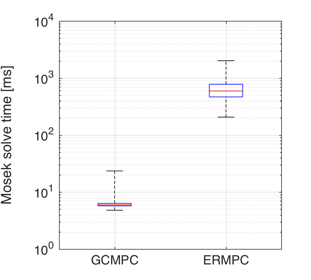
Figure 1: Computational time box plot of both GCMPC and ERMPC for uniformly distributed states with $||x||_{\infty}\leq 0.5$

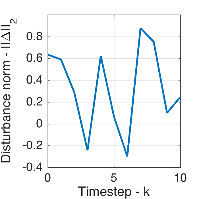
(a)

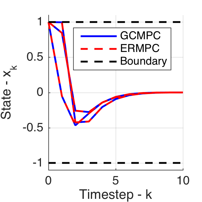
(b)

(c)

Figure 2: Simulation results for GCMPC and ERMPC controllers. (a) Simulated disturbance norm $||\Delta||_{2}$; (b) Disturbed closed-loop state $x_{k}$; (c) Executed control inputs $u_{k}$.

An infinite horizon positive definite solution $S$ exists to the GCC problem for $\epsilon_{k}\equiv\epsilon\in(0,0.0220)$ and $\epsilon=0.0180$ provides the optimal stabilizing solution, given by

$$S_{k}\equiv S=\begin{bmatrix}31.4751&-0.9359&-20.6124\\ -0.9359&5.7340&-1.3900\\ -20.6124&-1.3900&16.5017\end{bmatrix}$$ (54)

and

$$K_{k}\equiv K=\begin{bmatrix}1.1801&0.2151&-0.5076\\ 0.7401&-0.8385&0.5162\end{bmatrix}$$ (55)

whereas the GCMPC cost matrix $\bar{R}_{k}$ is

$$\bar{R}_{k}\equiv\bar{R}=\begin{bmatrix}123.22&133.78\\ 133.78&197.26\end{bmatrix}$$ (56)

and $\widetilde{K}$, a second order nil-potent controller, is

$$\widetilde{K}=\begin{bmatrix}11.5&-6&-6\\ 1.1&0&0\end{bmatrix}$$ (57)

The resulting optimization problems were solved in a minimum of $4.8ms$ and a maximum of $23.5ms$ for the GCMPC and a minimum of $206.77ms$ and a maximum of $2021.5ms$ for the ERMPC on a $2.5Ghz$ i7-4980HQ with $16Gb$ of RAM. The computational time distributions is shown in Figure 1, where it is possible to see that the GCMPC is on average two orders of magnitude faster than the ERMPC.

Figure 2 shows the simulation results of both controllers for an initial state $x_{0}=[1,1,1]^{T}$. The controlled system was subject to a uniformly distributed disturbance $\Delta_{k}\in[-1,1]$, shown in Figure 2(a)). The GCMPC successfully maintained the system bounded and stabilized with the an equivalent performance of the optimal ERMPC, as shown in Figure 2(b).

V CONCLUSIONS

In this paper we have proposed a constrained guaranteed cost robust model predictive controller for uncertain discrete time systems. Such controller provides an upper bound to the quadratic cost functional and ensures feasibility of states and control inputs within a prediction horizon for a system subject to a quadratically bound multiplicative uncertainty. This problem class was only tractable though vertex enumeration of a polytopic approximation of the uncertainty set.

The proposed approach is computationally more efficient than enumeration-based techniques and executed on average two orders of magnitude faster for this paper numerical example. It also requires only a QCQP optimization, which results in lower-complexity solutions than those of LMI-based guaranteed cost approaches based on SDP optimizations.

References

[1]
A. Alessio and A. Bemporad, “A survey on explicit model predictive control,”
in Nonlinear model predictive control. Springer, 2009, pp. 345–369.
[3]
T. A. Badgwell and S. J. Qin, “Model-predictive control in practice,”
Encyclopedia of Systems and Control, pp. 756–760, 2015.
[4]
A. Bemporad, F. Borrelli, and M. Morari, “Min-max control of constrained
uncertain discrete-time linear systems,” Automatic Control, IEEE
Transactions on, vol. 48, no. 9, pp. 1600–1606, 2003.
[5]
A. Bemporad and M. Morari, “Robust model predictive control: A survey,” in
Robustness in identification and control. Springer, 1999, pp. 207–226.
[6]
S. Boyd and L. Vandenberghe, Convex Optimization. New York, NY, USA: Cambridge University Press, 2004.
[7]
E. F. Camacho and C. B. Alba, Model predictive control. Springer Science & Business Media, 2013.
[8]
Y. Gao and K. T. Chong, “The explicit constrained min-max model predictive
control of a discrete-time linear system with uncertain disturbances,”
Automatic Control, IEEE Transactions on, vol. 57, no. 9, pp.
2373–2378, 2012.
[9]
H. Genceli and M. Nikolaou, “Robust stability analysis of constrained l1-norm
model predictive control,” AIChE Journal, vol. 39, no. 12, pp.
1954–1965, 1993.
[12]
H. V. Henderson and S. R. Searle, “On deriving the inverse of a sum of
matrices,” Siam Review, vol. 23, no. 1, pp. 53–60, 1981.
[13]
R. E. Kalman et al., “Contributions to the theory of optimal control,”
Bol. Soc. Mat. Mexicana, vol. 5, no. 2, pp. 102–119, 1960.
[14]
E. C. Kerrigan and J. M. Maciejowski, “Feedback min-max model predictive
control using a single linear program: robust stability and the explicit
solution,” International Journal of Robust and Nonlinear Control,
vol. 14, no. 4, pp. 395–413, 2004.
[15]
J. Löfberg, “Approximations of closed-loop minimax MPC,” in
Decision and Control, 2003. Proceedings. 42nd IEEE Conference on,
vol. 2. IEEE, 2003, pp. 1438–1442.
[16]
——, “Yalmip: A toolbox for modeling and optimization in matlab,” in
Computer Aided Control Systems Design, 2004 IEEE International
Symposium on. IEEE, 2004, pp.
284–289.
[17]
——, “Automatic robust convex programming,” Optimization methods and
software, vol. 27, no. 1, pp. 115–129, 2012.
[18]
J. Mattingley and S. Boyd, “Cvxgen: A code generator for embedded convex
optimization,” Optimization and Engineering, vol. 13, no. 1, pp.
1–27, 2012.
[19]
I. R. Petersen, D. C. McFarlane, and M. A. Rotea, “Optimal guaranteed cost
control of discrete-time uncertain linear systems,” International
Journal of Robust and Nonlinear Control, vol. 8, no. 8, pp. 649–657, 1998.
[20]
S. J. Qin and T. A. Badgwell, “A survey of industrial model predictive control
technology,” Control engineering practice, vol. 11, no. 7, pp.
733–764, 2003.
[21]
F. Quelho Rossi, R. Waschburger, and R. Kawakami Harrop Galvao, “Regions of
guaranteed cost for lmi-based robust model predictive controllers for systems
with uncertain input delay,” in Control and Fault-Tolerant Systems
(SysTol), 2013 Conference on. IEEE,
2013, pp. 584–589.
[22]
J. Rawlings, E. Meadows, and K. Muske, “Nonlinear model predictive control: A
tutorial and survey,” Advanced Control of Chemical Processes, pp.
203–214, 1994.
[23]
D. Rosinová, V. Veselỳ, and V. Kučera, “A necessary and
sufficient condition for static output feedback stabilizability of linear
discrete-time systems,” Kybernetika, vol. 39, no. 4, pp. 447–459,
2003.
[24]
P. Scokaert and D. Mayne, “Min-max feedback model predictive control for
constrained linear systems,” Automatic Control, IEEE Transactions on,
vol. 43, no. 8, pp. 1136–1142, 1998.
[25]
M. H. Terra, J. P. Cerri, and J. Y. Ishihara, “Optimal robust linear quadratic
regulator for systems subject to uncertainties,” Automatic Control,
IEEE Transactions on, vol. 59, no. 9, pp. 2586–2591, 2014.
[26]
L. Xie and Y. C. Soh, “Control of uncertain discrete-time systems with
guaranteed cost,” in Decision and Control, 1993., Proceedings of the
32nd IEEE Conference on. IEEE, 1993,
pp. 56–61.