Optimal Weights For Measuring Redshift Space Distortions in Multi-tracer Galaxy Catalogues

Abstract

Since the volume accessible to galaxy surveys is fundamentally limited, it is extremely important to analyse available data in the most optimal fashion. One way of enhancing the cosmological information extracted from the clustering of galaxies is by weighting the galaxy field. The most widely used weighting schemes assign weights to galaxies based on the average local density in the region (FKP weights) and their bias with respect to the dark matter field (PVP weights). They are designed to minimize the fractional variance of the galaxy power-spectrum. We demonstrate that the currently used bias dependent weighting scheme can be further optimized for specific cosmological parameters. We develop a procedure for computing the optimal weights and test them against mock catalogues for which the values of all fitting parameters, as well as the input power-spectrum are known. We show that by applying these weights to the joint power-spectrum of Emission Line Galaxies and Luminous Red Galaxies from the Dark Energy Spectroscopic Instrument survey, the variance in the measured growth rate parameter can be reduced by as much as 36 per cent.

1 Introduction

Future galaxy redshift surveys, such as the Dark Energy Spectroscopic Instrument survey (DESI; Schlegel et al., 2011; Levi et al., 2013), the Extended Baryon Oscillation Spectroscopic survey (eBOSS; Schlegel et al., 2009), the Euclid satellite surveys (Laureijs et al., 2011), and the Wide Field Infrared Survey Telescope surveys (WFIRST; Spergel et al., 2013) will cover vast cosmological volumes with a high number density of galaxies. Since the available cosmic volume is fundamentally limited a lot of effort is going into developing optimal ways of analysing galaxy clustering data (see e.g., Eisenstein et al., 2007; Blazek et al., 2014; Bianchi et al., 2015; Scoccimarro, 2015; Slepian & Eisenstein, 2016).

One way of improving the variance of measured 2-point statistics is to weight the galaxy field to achieve the optimal signal-to-noise. The most commonly used weighting scheme is the one developed by Feldman, Kaiser & Peacock (1994, hereafter FKP), which is used in all analyses employing 2-point statistics (see e.g., Percival et al., 2001; Reid et al., 2010; Blake et al., 2011; Anderson et al., 2012; Ross et al., 2013; Beutler et al., 2011, 2012, 2014; Gil-Marín et al., 2015). The FKP weights,

$$w_{\mathrm{FKP}}(\mn@boldsymbol{r})\propto\dfrac{1}{1+\overline{n}(\mn@boldsymbol{r})P(\mn@boldsymbol{k})},$$ (1)

where $\overline{n}(\mn@boldsymbol{r})$ is the average number density of galaxies at a position $\mn@boldsymbol{r}$ and $P(\mn@boldsymbol{k})$ is the power-spectrum at a wavelength of interest $\mn@boldsymbol{k}$, are straightforward to apply and reduce the variance of the measured power-spectrum when the completeness of the galaxy sample is significantly non-uniform.

Percival, Verde & Peacock (2004, hereafter PVP) further optimized the FKP scheme for samples that include galaxies with a range of biases with respect to the dark matter. If the number density is uniform the PVP weights are

$$w_{\mathrm{PVP}}\propto b,$$ (2)

where $b$ is the bias with respect to the dark matter, and will minimize the fractional variance in the measured power-spectrum.

If a galaxy sample covers such a wide redshift range that the effects of cosmic evolution are significant, the measured power-spectrum will be a weighted average of power spectra at different redshifts within that range. Since the sensitivity of the power-spectrum to cosmological parameters also varies with redshift, it is possible to construct redshift dependent weights which maximize the constraining power of the measured power-spectrum for specific cosmological parameters. This optimal weighting scheme obviously depends on which cosmological parameters we want to optimize. Recently, Zhu, Padmanabhan & White (2015) derived redshift weights that optimize the measurement of the Baryon Acoustic Oscillation (BAO) Peak position, while Ruggeri et al. (2016) derived similar weights that optimize the Redshift Space Distortion (RSD) parameter. Both works built on the formalism developed in Tegmark, Taylor & Heavens (1997).

Future surveys will observe emission line galaxies (ELGs), luminous red galaxies (LRGs), and quasars (QSOs), in overlapping volumes. Computing power spectra of all tracers individually is suboptimal as important information encoded in the cross-correlation of the tracers will be lost. A promising way of taking advantage of the presence of multiple tracers was proposed in McDonald & Seljak (2009). The method, however, has not yet been implemented in practice and will only result in a significant improvement in constraining power when the number density of tracers is high (which is not the case e.g. in the eBOSS survey). Computing all auto and cross power spectra is possible (Ross et al., 2012) but will require accurate estimation of large covariance matrices which may be problematic for future surveys (Pope & Szapudi, 2008; Schneider et al., 2011; de Putter et al., 2012; Xu et al., 2012; de la Torre et al., 2013; Mohammed & Seljak, 2014; Paz & Sanchez, 2015; Grieb et al., 2016; Pearson & Samushia, 2016). The most straightforward way is to compute a single power-spectrum for all tracers while differentially weighting them to achieve optimal signal-to-noise by applying the PVP weights.

While the PVP weights are designed to minimize the fractional variance in the power-spectrum, this does not necessarily translate into minimal variance on measured cosmological parameters. A good example of this is the growth rate parameter, $f$. The growth rate is measured from an anisotropic signature in the power-spectrum which is more pronounced for low biased tracers. The power-spectrum signal on the other hand is stronger in the high biased tracers. The weights in equation (2) upweight high bias galaxies to achieve the optimal power-spectrum signal, but the measured power-spectrum becomes less sensitive to $f$. The optimal weighting for the growth rate parameter must counterbalance these two tendencies by producing a power-spectrum with a small (not necessarily minimal) variance that is at the same time sensitive enough to the $f$ parameter.

In this work we generalize the PVP weighting scheme to minimize the variance of specific cosmological parameters measured from the power-spectrum (section 2). We assume that the galaxy samples will be analysed in narrow redshift bins of $\delta z\sim 0.1$, eliminating the need to consider the redshift evolution weights (Zhu et al., 2015; Ruggeri et al., 2016) as the effect will be small. We test our new weighting scheme on mock catalogues of the eBOSS and DESI surveys (section 3) and show that they could improve the variance of the measured $f$ parameter by up to 36 per cent. As expected, the optimal weights differ for different cosmological parameters (section 4). This weighting scheme is straightforward to compute and implement and should result in reduced variance on cosmological parameters measured from future galaxy surveys (section 5).

2 Optimal Weighting

For simplicity, we will assume that galaxies of two types with densities $n_{1}(\mn@boldsymbol{r})$ and $n_{2}(\mn@boldsymbol{r})$ are present in an overlapping volume and the average number densities $\overline{n}_{1}$ and $\overline{n}_{2}$ do not vary significantly within the volume. The formalism is easy to generalize for more than two tracers and varying number densities. If we assign weights $w_{1}$ and $w_{2}$ to these galaxies, then the number density of the combined field is

$$n(\mn@boldsymbol{r})=w_{1}n_{1}(\mn@boldsymbol{r})+w_{2}n_{2}(\mn@boldsymbol{r})$$ (3)

and the overdensity field is

$$\delta(\mn@boldsymbol{r})\equiv\frac{n(\mn@boldsymbol{r})-\overline{n}}{\overline{n}}=A_{1}\delta_{1}(\mn@boldsymbol{r})+A_{2}\delta_{2}(\mn@boldsymbol{r}),$$ (4)

where the overdensities are defined by

$$\delta_{i}(\mn@boldsymbol{r})=\frac{n_{i}(\mn@boldsymbol{r})-\overline{n}_{i}}{\overline{n}_{i}},$$ (5)

and

$$A_{i}=\frac{w_{i}\overline{n}_{i}}{w_{1}\overline{n}_{1}+w_{2}\overline{n}_{2}}$$ (6)

is the weighted fractional density. We will assume the weights to be normalised by $w_{1}+w_{2}=1$. This will shorten some of our formulas, although in practice only the ratio of weights is relevant. The power-spectrum of the overdensity field,

$$P(\mn@boldsymbol{k})\equiv\left|\widetilde{\delta}(\mn@boldsymbol{k})\right|^{2},$$ (7)

can be estimated from the squared modulus of the Fourier transform,

$$\widetilde{\delta}(\mn@boldsymbol{k})=\displaystyle\int\!\mathrm{d}\mn@boldsymbol{r}\,\mathrm{e}^{-i\mn@boldsymbol{kr}}\delta(\mn@boldsymbol{r}),$$ (8)

We will assume that the overdensity fields are Gaussian (this is a common assumption when deriving optimal weights) with

$$\left<\widetilde{\delta}_{i}(\mn@boldsymbol{k})\widetilde{\delta}^{\star}_{j}(\mn@boldsymbol{k})\right>=\left[\left(b_{i}+\mu^{2}f\right)\left(b_{j}+\mu^{2}f\right)P_{\mathrm{m}}(k)+\frac{\delta^{\text{\tiny C}}_{ij}}{\overline{n}_{i}}\right]V_{\mathrm{s}},$$ (9)

where the angular brackets denote the expectation value, $\delta^{\text{\tiny C}}$ is a Kronecker delta function, $V_{\mathrm{s}}$ is the survey volume, and $P_{\mathrm{m}}(k)$ is the matter power-spectrum that can be computed in any given cosmological model (Kaiser, 1987; Hamilton, 1997). The last term in equation (9) is the Shot-Noise term due to the sampling of the overdensity field with a finite number of galaxies (FKP). For the weighted field in equation (4) this results in

$$P(\mn@boldsymbol{k})=\left[\left(b_{\mathrm{eff}}^{w_{1}w_{2}}+\mu^{2}f\right)^{2}P_{\mathrm{m}}(k)+S^{w_{1}w_{2}}\right]V_{\mathrm{s}},$$ (10)

with the weighting dependent effective bias,

$$b_{\mathrm{eff}}^{w_{1}w_{2}}=A_{1}b_{1}+A_{2}b_{2},$$ (11)

and the shot noise term,

$$S^{w_{1}w_{2}}=\frac{A_{1}^{2}}{\overline{n}_{1}}+\frac{A_{2}^{2}}{\overline{n}_{2}}.$$ (12)

Since we assumed the overdensity field to be Gaussian, the variance of the galaxy power-spectrum estimator is simple to compute and is

$$\mathrm{Var}\left[P(\mn@boldsymbol{k})\right]\propto\left[\left(b_{\mathrm{eff}}^{w_{1}w_{2}}+\mu^{2}f\right)^{2}P_{\mathrm{m}}(k)+S^{w_{1}w_{2}}\right]^{2}$$ (13)

(FKP; PVP; Tegmark et al., 1997). The fractional variance in the galaxy power-spectrum is then

$$\frac{P(\mn@boldsymbol{k})}{\mathrm{Var}\left[P(\mn@boldsymbol{k})\right]}\propto\frac{\left(b_{\mathrm{eff}}^{w_{1}w_{2}}+\mu^{2}f\right)^{2}P_{\mathrm{m}}(k)}{\left[\left(b_{\mathrm{eff}}^{w_{1}w_{2}}+\mu^{2}f\right)^{2}P_{\mathrm{m}}(k)+S^{w_{1}w_{2}}\right]^{2}}.$$ (14)

This expression is minimized by

$$\begin{array}[]{@{}l}w_{1}=\dfrac{b_{1}}{b_{1}+b_{2}},\\ w_{2}=\dfrac{b_{2}}{b_{1}+b_{2}},\\ \end{array}$$ (15)

which, for constant number densities, is equivalent to PVP weighting.

The minimum fractional variance in the power-spectrum, however, does not necessarily correspond to the minimum variance in the cosmological parameters derived from the power-spectrum. The power-spectrum is most sensitive to the bias – $b_{\mathrm{eff}}$, growth rate – $f$, and the Alcock-Paczinsky parameters $\alpha_{\parallel}$ and $\alpha_{\perp}$ (Alcock & Paczynski, 1979; Kaiser, 1987). The dependence on $b$ and $f$ is already in equation (10), and the dependence on $\alpha_{\perp}$ and $\alpha_{\parallel}$ can be introduced by replacing

$$k\longrightarrow\dfrac{k}{\alpha_{\perp}}\left[1+\mu^{2}\left(\dfrac{\alpha_{\perp}^{2}}{\alpha_{\parallel}^{2}}-1\right)\right]^{1/2},$$ (16)

$$\mu\longrightarrow\dfrac{\mu\alpha_{\perp}}{\alpha_{\parallel}}\left[1+\mu^{2}\left(\dfrac{\alpha_{\perp}^{2}}{\alpha_{\parallel}^{2}}-1\right)\right]^{-1/2},$$ (17)

and dividing the power-spectrum by a factor of $\alpha_{\parallel}\alpha_{\bot}^{2}$ (Ballinger et al., 1996; Simpson & Peacock, 2010; Samushia et al., 2011). The Fisher information matrix of these parameters is

$$F_{ij}=\displaystyle{\int}\!\mathrm{d}\mn@boldsymbol{k}\,\frac{\partial P(\mn@boldsymbol{k})}{\partial\theta_{i}}\frac{1}{\mathrm{Var}\left[P(\mn@boldsymbol{k})\right]}\frac{\partial P(\mn@boldsymbol{k})}{\partial\theta_{j}},$$ (18)

where $\mn@boldsymbol{\theta}=(b_{\mathrm{eff}},f,\alpha_{\parallel},\alpha_{\bot})$ is a parameter vector, and the integration is over all wavevectors, the power-spectrum measurements of which where used in the analysis. The inverse of the Fisher matrix gives a covariance matrix

$$\mathsf{C}=\mathsf{F}^{-1}$$ (19)

and the diagonal elements of the covariance matrix correspond to the expected variance of the parameters measured from the power-spectrum. Because of the presence of the derivative terms (that also depend on the weights) in equation (18) the weighting scheme that minimizes the variance of the power-spectrum does not necessarily minimize the diagonal elements of the covariance matrix in equation (19).

A simple analytic solution for the optimal weights in this case does not exist, but they are relatively straightforward to find numerically. To find the optimal weights we numerically compute the variance and the derivatives in equation (18) and take the integral over the wavevectors of interest. We then numerically find the weights that minimize the diagonal elements of the inverse Fisher matrix of equation (19). These weights will in general be different for each parameter. In the tradition of FKP and PVP, we refer to these as PSG weights in what follows.

3 Data and Measurement Procedures

3.1 The Sample

In order to test our weighting scheme, we generated lognormal mock catalogues (Coles & Jones, 1991) giving us control over the input power-spectrum and linear growth rate.

We computed the matter power-spectrum using the camb software (Lewis, Challinor & Lasenby, 2000) via the web interface hosted at LAMBDA for a spatially flat $\Lambda$CDM cosmology with $\Omega_{\mathrm{M}}=0.276$, and $\Omega_{\mathrm{b}}h^{2}=0.0226$. We use the fiducial value of

$$f(\Omega_{\mathrm{M}},z)\approx\Omega_{\mathrm{M}}^{0.6}(z),$$ (20)

where

$$\Omega_{\mathrm{M}}(z)=\dfrac{\Omega_{\mathrm{M},0}(1+z)^{3}}{\Omega_{\mathrm{M},0}(1+z)^{3}+\Omega_{\Lambda,0}},$$ (21)

which is the value predicted by general relativity (Peebles, 1980; Martínez & Saar, 2002).

Our lognormal code was largely based on the description given in Weinberg & Cole (1992) and Appendix A of Beutler et al. (2011), with modifications required to obtain a distribution of two tracers cross-correlated by the same underlying matter field.

We started by distributing the power to two grids – one for LRGs and one for ELGs – in $k$-space as

$$P(\mn@boldsymbol{k})=\left(b_{i}+\mu^{2}f\right)^{2}P_{\mathrm{m}}(k),$$ (22)

where $\mu=k_{z}/k$ and $b_{i}$ is the bias of LRGs or ELGs for the redshift bin. This was assigned to the real part only, with the imaginary part being set to zero. After performing inverse Fourier transforms using the complex-to-real transform in the Fastest Fourier Transform in the West (fftw) library (Frigo & Johnson, 2005), we took the resulting correlation functions and calculated $\ln[1+\xi^{i}(\mn@boldsymbol{r})]$ at each grid point, then performed real-to-complex transforms. The result of these transforms, $P^{i}_{\mathrm{LN}}(\mn@boldsymbol{k})$, was then normalized by the number of grid points since fftw produces the unnormalized Fourier transform.

At this stage, we took the ratio of the $P^{i}_{\mathrm{LN}}(\mn@boldsymbol{k})$ at each grid point in $k$-space and stored that in memory. We then constructed Gaussian random realizations by drawing from a normal distribution, centred on zero, with $\sigma=\sqrt{\max\{0,\mathrm{Re}[P_{\mathrm{LN}}(\mn@boldsymbol{k})]\}/2}$, at each grid point for both the real and imaginary parts, in order to obtain a well behaved power-spectrum (Weinberg & Cole, 1992). We took care that $\delta_{\mathrm{LN}}(-\mn@boldsymbol{k})=\delta_{\mathrm{LN}}^{\ast}(\mn@boldsymbol{k})$, and that the values at grid points whose indices are combinations of zero and $N_{i}/2$, where $N_{i}$ is the number of grid points in dimension $i$, were purely real. This ensured that when we inverse Fourier transformed $\delta_{\mathrm{LN}}(\mn@boldsymbol{k})$, the result was purely real. We only did the random draw for the higher bias tracer, then using the ratio previously calculated, we scaled the random realization to obtain the values on the grid for the lower bias tracer. In this way, we were able to effectively obtain mock samples with two tracers, each following the same underlying matter distribution.

The last step was then to take the inverse Fourier transforms of the random realization for the higher bias tracer, and the scaled realization for the lower bias tracer. This resulted in overdensity fields for both tracers, $\delta_{i}(\mn@boldsymbol{r})$, having zero mean and variance $\sigma_{\mathrm{G}}^{2}$. From these overdensity fields we calculated the lognormal density field

$$\delta_{\mathrm{LN},i}(\mn@boldsymbol{r})=\exp\left[\delta_{i}(\mn@boldsymbol{r})-\sigma_{\mathrm{G}}^{2}/2\right].$$ (23)

This was then multiplied by the average number of galaxies per cell to give the desired number density, and Poisson sampled to create our final galaxy catalogues, placing the galaxies randomly within a given cell.

Table 1: Mock catalogue properties. Column 1 list the redshift range. Columns 2, 3 and 4 list the volume of the cube and the number denisties for LRGs and ELGs to match the eBOSS survey, respectively. Columns 5, 6, and 7 list the volume of the cube and the number densities for LRGs and ELGs to match that expected in the DESI survey, respectively. Columns 8 and 9 list the biases for the LRGs and ELGs, respectively. Lastly, column 7 lists the dimensionless linear growth rate for the redshift bin.

Redshift	$V_{\mathrm{eBOSS}}$	$\bar{n}_{\mathrm{LRG,eBOSS}}$	$\bar{n}_{\mathrm{ELG,eBOSS}}$	$V_{\mathrm{DESI}}$	$\bar{n}_{\mathrm{LRG,DESI}}$	$\bar{n}_{\mathrm{ELG,DESI}}$	$b_{\mathrm{LRG}}$	$b_{\mathrm{ELG}}$	$f$
	($h^{-3}\mathrm{Gpc}^{3}$)	$(10^{-4}h^{3}\mathrm{Mpc^{-3}})$	$(10^{-4}h^{3}\mathrm{Mpc^{-3}})$	($h^{-3}\mathrm{Gpc}^{3}$)	$(10^{-4}h^{3}\mathrm{Mpc^{-3}})$	$(10^{-4}h^{3}\mathrm{Mpc^{-3}})$
$0.6\leq z<0.7$	0.272	0.772	1.345	2.538	4.589	1.704	2.339	1.376	0.759
$0.7\leq z<0.8$	0.325	0.642	2.051	3.031	4.555	10.482	2.450	1.441	0.787
$0.8\leq z<0.9$	0.374	0.330	1.559	3.491	2.655	7.711	2.563	1.508	0.812
$0.9\leq z<1.0$	0.419	0.091	0.586	3.914	0.973	7.490	2.678	1.575	0.834

We generated 1024 mock catalogues for four redshift bins in $0.6<z<1.0$. They contained two tracers designed to mimic LRGs and ELGs. This led to a total of 4096 mock catalogues with number densities to match those expected in the eBOSS survey, and 4096 with number densities to match those expected in the DESI survey. Table 1 lists the specific properties for the mock catalogues. For the eBOSS mocks, the number densities were calculated from information in Zhao et al. (2016). The volumes were calculated for the 1500 deg² region were the ELGs and LRGs would overlap. The DESI number densities were calculated from information in the DESI Science Final Design Report (DESI Collaboration, 2016), and the volumes assume the 14,000 deg² baseline survey footprint. The biases for the different redshift bins were given by Dawson et al. (2016).

To have a clean separation between number density dependent and bias dependent weights, our mock catalogues have a constant number density. Since there are no number density gradients, the FKP weights reduce to a simple uniform weighting (see section 4), meaning any improvements are only coming from the differential weighting of tracers based on their bias.

3.2 Measuring the Power-Spectrum

We followed the general methods of FKP for measuring the power-spectrum from our mock catalogues. We generated random catalogues with 10 or 30 times the number of each tracer for the DESI and eBOSS mocks, respectively. The galaxies and randoms were binned using cloud-in-cell interpolation (Birdsall & Fuss, 1969) with one of the three different weighting schemes – see section 4 for details. Since we used a discrete Fourier transform of boxes with a finite linear size $L=V^{1/3}$ (see Table 1 for volumes), our $\tilde{\delta}(\mn@boldsymbol{k})$ (and correspondingly $P(\mn@boldsymbol{k})$ measurements) were given on a discrete cubic grid with a resolution of $2\pi/L$. To compress this information we computed the spherically averaged power-spectrum monopole and quadrupole ($l=0$, 2) in 24 bins of width $\Delta k=0.008$ for $0.008\leq k\leq 0.2$ via

$$P_{l}(k)=\dfrac{2l+1}{2}\sum\left|\widetilde{\delta}(\mn@boldsymbol{k})\right|^{2}\mathcal{P}_{l}\left[\mu(\mn@boldsymbol{k})\right]G^{2}(\mn@boldsymbol{k}),$$ (24)

where the sum is over all wavevectors in the range $k-\Delta k/2\leq|\mn@boldsymbol{k}|<k+\Delta k/2$, $\mathcal{P}_{l}(x)$ are the Legendre polynomials, and $G(\mn@boldsymbol{k})$ is a grid correction term

$$G(\mn@boldsymbol{k})=\prod_{i}\left[\mathrm{sinc}(\Delta L_{i}k_{i})\right]^{-2},$$ (25)

with $\mathrm{sinc}(x)=\sin(x)/x$, $\Delta L_{i}=L_{i}/N_{i}$, $i$ denotes one of the three Cartesian coordinates, $L_{i}$ is the length of the cube in that coordinate direction, and $N_{i}$ is the corresponding number of grid points.

We only considered the power-spectrum measurements below $k\sim 0.2$ allowing us to safely ignore the non-linear effects at higher wavevectors which are difficult to model and are usually excluded from the analysis. Even though our Fisher matrix predictions in section 2 implicitly assumed that each $P(\mn@boldsymbol{k})$ measurement would be analysed individually without reducing them to the multipoles, we do not expect this to be a big effect as a number of recent studies showed that reducing the power-spectrum to the first few even multipoles retains most of the information (Taruya et al., 2011; Kazin et al., 2012).

The measurements resulting from equation (24) were then corrected for shot noise

$$S_{l}(k)=\dfrac{1}{N_{k}}\left(\sum_{\mathrm{gal}}w_{i}^{2}+\alpha^{2}\sum_{\mathrm{ran}}w_{i}^{2}\right)\sum_{\mu}\mathcal{P}_{l}(\mu),$$ (26)

where the sum is over the same modes, with $\alpha=\sum_{\mathrm{gal}}w_{i}/\sum_{\mathrm{ran}}w_{i}$, and then normalized by

$$I=V_{\mathrm{s}}\left(\overline{n}_{\mathrm{LRG}}w_{\mathrm{LRG}}+\overline{n}_{\mathrm{ELG}}w_{\mathrm{ELG}}\right)^{2}.$$ (27)

Since the power-spectrum multipoles in equation (24) were computed as a discrete sum over a finite number of wavevectors, modelling them as angular integrals over the theoretical power-spectrum of equation (22) would be inaccurate. To model the $\mn@boldsymbol{k}$-grid discreteness effects we distributed the model power to the same grid used to calculate the power-spectrum from the mocks and binned it according to equation (24) to give $P^{\mathrm{grid}}_{l}(k)$. We then adjusted the measured value,

$$P_{l}(k)\longrightarrow P_{l}(k)-\left[P^{\mathrm{grid}}_{l}(k)-P^{\mathrm{int}}_{l}(k)\right],$$ (28)

where

$$P^{\mathrm{int}}_{l}(k)=\dfrac{2l+1}{2}\displaystyle\int\limits_{-1}^{1}\!\left(b_{\mathrm{eff}}^{w_{1}w_{2}}+\mu^{2}f\right)^{2}P_{\mathrm{m}}(k)\mathcal{P}_{l}(\mu)~{}\mathrm{d}\mu,$$ (29)

is the integrated power-spectrum (Blake et al., 2011; Beutler et al., 2014). This effect (correction term in the brackets) is extremely small for the monopole, so in practice we only applied the correction to the quadrupole.

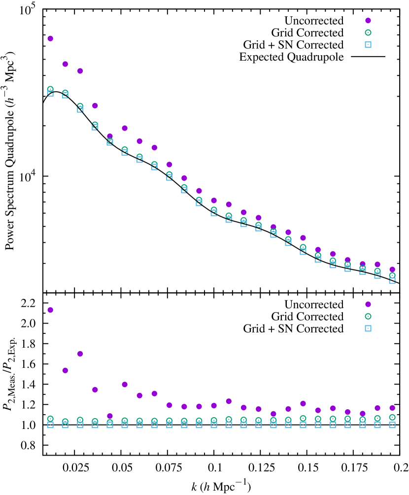
Figure 1: Here we show the effects of the discreteness of the grid on the quadrupole for the number densities and volume of the first redshift bin of eBOSS. The solid circles (purple) show the model power after being distributed to the grid, binned as in equation (24) and adding the expected shot noise calculated as in equation (26). The open circles (green) show the effects of the correction in equation (28). It is clear that even after applying that correction, there is a small positive bias (${\sim}5$ per cent). The open squares (light blue) show the measured quadrupole after correcting for the discreteness in the shot-noise as well, at which point we have recovered the expected quadrupole quite well.

We would like to emphasize that, given the small volume of our mocks (especially the eBOSS mocks), the $\mn@boldsymbol{k}$-grid discreteness effects also had to be accounted for when computing the shot-noise correction. Even though integrals over higher order Legendre polynomials are zero, the discrete sum over $\mu$ in equation (26) is nonzero. This implies that the shot-noise corrections have to be applied not only to the monopole but to the higher order multipoles of the power-spectrum as well. Fig. 1 explicitly shows these effects on the quadrupole for the first redshift bin eBOSS mocks. We found that ignoring the effects in equation (28) can bias the quadrupole by ${\sim}27$ per cent on average, and significantly more so at low wavenumbers. While significantly smaller, ignoring the discreteness effects in the shot-noise – equation (26) – can bias the quadrupole by ${\sim}5$ per cent. We note that the size of these corrections decrease for increased volume, and the shot-noise additionally decreases for increased number densities. For example, in the first redshift bin of the DESI mocks, the effect in equation (28) drops to ${\sim}13$ per cent on average, while the shot-noise causes a bias of less than 1 per cent.

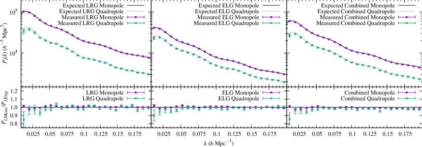
Figure 2: Comparison of the expected power-spectrum monopole and quadrupole with the measured values after applying all corrections for LRGs (left), ELGs (middle) and the combined sample (right) with equal weighting in the first redshift bin with eBOSS number densities. The plotted error bars are $\sqrt{C_{ii}/N}$ where $C_{ii}$ are the diagonal elements of the sample covariance matrix, and $N$ is the number of mocks.

Fig. 2 shows a detailed comparison of the power-spectrum which we expected to recover and the power-spectrum that we actually measured for the first redshift bin ($0.6\leq z<0.7$) with the eBOSS number densities and volume. We explicitly show the recovered power for each tracer individually as confirmation of our scaling procedure (see section 3.1). We also note that we recovered the expected power-spectrum extremely well for the other eBOSS redshift bins and for the DESI volumes as well.

3.3 Parameter Estimation

We model the measured power-spectrum multipoles as

$$P_{l}(k)=\dfrac{2l+1}{2\alpha_{\perp}^{2}\alpha_{\parallel}}\displaystyle\int\limits_{-1}^{1}\!\mathrm{d}\mu~{}P(k,\mu)\mathcal{P}_{l}(\mu),$$ (30)

where

$$P(k,\mu)=\left(b_{\mathrm{eff}}^{w_{1}w_{2}}+\mu^{2}f\right)^{2}P_{\mathrm{m}}(k),$$ (31)

and $k$, and $\mu$ depend on $\alpha_{\perp}$ and $\alpha_{\parallel}$ as in equations (16) and (17). The shape of the power-spectrum is fixed, while the four parameters $b_{\mathrm{eff}}^{w_{1}w_{2}}$, $f$, $\alpha_{\parallel}$, $\alpha_{\perp}$ are free.

In order to find the best-fitting parameters, we used a Markov-Chain Monte Carlo (MCMC) method with the Metropolis-Hastings algorithm (Hastings, 1970) to find the posterior likelihood of the free parameters. In all our MCMC chains the mean values of the parameters were very close to the input values and the likelihood surfaces were close to Gaussian. We computed the variance of each parameter from the MCMC mocks and compared the resulting values for all the parameters for a specific set of weights to other weighting schemes to see if the PSG weights actually yield the tightest constraints.

4 Comparison with Other Weighting Schemes

In order to test the weights purely from the stand point of relative weighting of tracers, our mock catalogues have uniform number densities through out, and only two types of tracers with constant biases. In what follows, for brevity we will quote weights as pairs in the form $(w_{\mathrm{LRG}},w_{\mathrm{ELG}})$.

Table 2: The PSG weights for the free parameters in our model. Column 1 indicates the target survey for the weights. Column 2 gives the redshift range. Columns 3, 4, 5, and 6 give the optimal weights for each parameter individually.

Survey	Redshift Range	$b$	$f$	$\alpha_{\perp}$	$\alpha_{\parallel}$
DESI	$0.6\leq z<0.7$	$(0.279,0.721)$	$(0.207,0.793)$	$(0.546,0.454)$	$(0.464,0.536)$
	$0.7\leq z<0.8$	$(0,1)$	$(0,1)$	$(0.516,0.484)$	$(0.347,0.653)$
	$0.8\leq z<0.9$	$(0,1)$	$(0,1)$	$(0.547,0.453)$	$(0.429,0.571)$
	$0.9\leq z<1.0$	$(0,1)$	$(0,1)$	$(0.568,0.432)$	$(0.472,0.528)$
eBOSS	$0.6\leq z<0.7$	$(0.427,0.573)$	$(0.367,0.633)$	$(0.589,0.411)$	$(0.547,0.453)$
	$0.7\leq z<0.8$	$(0.405,0.595)$	$(0.326,0.674)$	$(0.589,0.411)$	$(0.544,0.456)$
	$0.8\leq z<0.9$	$(0.447,0.553)$	$(0.385,0.615)$	$(0.597,0.403)$	$(0.559,0.441)$
	$0.9\leq z<1.0$	$(0.501,0.499)$	$(0.471,0.529)$	$(0.609,0.391)$	$(0.580,0.420)$

Because of the simplified nature of our mocks, the FKP weights are then simply $(0.5,0.5)$ regardless of the target survey or redshift bin. Similarly, the PVP weights will be the same regardless of the target survey or redshift bin and will result in upweighting the LRGs as they have a higher bias – see equation (15). Since $b_{\mathrm{LRG}}\simeq 1.7b_{\mathrm{ELG}}$ at all redshifts (Dawson et al., 2016; Zhao et al., 2016), the PVP weights are $(0.63,0.37)$. The PSG weights vary from redshift bin to redshift bin somewhat, and from survey to survey, due to the varying relative number densities of the tracers. They are also different for different model parameters. We compute them following the numerical procedure outlined in section 2.

Table 2 summarizes the PSG weights for the different redshift bins of the two surveys. In some cases the PSG weights are close to the FKP or PVP weights, but in many cases differ substantially. It is also interesting to note that for the DESI mocks, the PSG weights actually imply that above a redshift of 0.7, it would be better to consider only the ELGs when measuring the RSD parameters. However, this does not mean that the LRG and cross power spectra do not contain additional information. The LRG, ELG and cross power spectra (with appropriate covariance matrices) in principle contain all of the information. Our weighting in some sense gives the most optimal mixture (best principle component) of the three if they were to be reduced to a single power-spectrum, but other orthogonal mixtures (next principle components) will of course contain additional information. Having $w_{\mathrm{LRG}}=0$ simply means that a pure ELG power-spectrum is better at constraining the $f$ parameter compared to any other mixture of ELGs and LRGs.

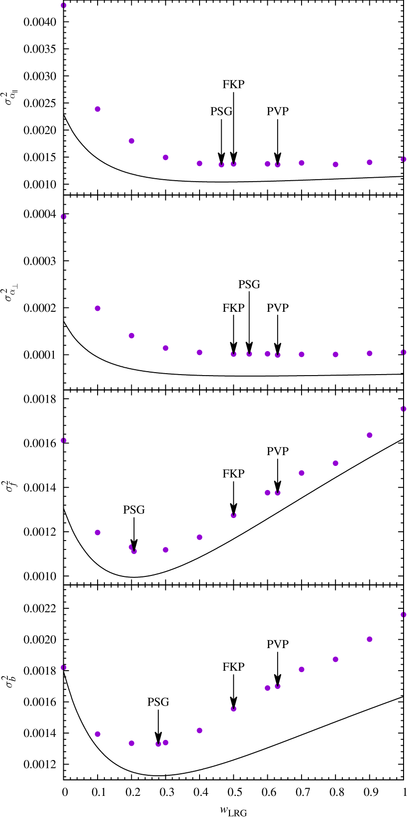
Figure 3: Variance of each parameter versus the relative weight of the LRGs for the first redshift bin of the DESI mocks. The points associated with the FKP, PVP, and PSG weights have been labelled. The solid lines are the theoretical predictions for the variance. In general, the points follow the shapes of the theoretical curves. For $b$ and $f$, the PSG weights are clearly optimal, while for $\alpha_{\perp}$ and $\alpha_{\parallel}$ the variance is flat for a broad range of weights leading all weighting schemes to perform equally well.

Fig. 3 shows the resulting variance of the four parameters for a variety of weights starting at $(0.0,1.0)$ – only ELGs – and going to $(1.0,0.0)$ – only LRGs – in steps of 0.1, as well the FKP, PVP and PSG weighting schemes, in the first redshift bin for the DESI mocks. The points show the actual variance in measured parameter values from the mocks, while the lines show theoretical predictions based on our Fisher matrix formalism.

It is remarkable that the measured variances follow the theoretical predictions very closely. The fact that the minimums of the theoretical curves match well to the measured minimum variance values shows that the methods presented in section 2 are sufficiently accurate and could, in principle, be applied to any parameter that needs to be constrained, so long as non-linear effects can be safely ignored.

For the remaining redshift bins of the DESI mocks and all redshift bins of the eBOSS mocks, we simply report the variance of each parameter for the FKP, PVP and PSG weights. These results are summarized in Table 3. It can be seen that the PSG weights derived here essentially always produce smaller variances on their associated parameter. However, there are some cases in which the PSG weights produce the same or larger variances than the FKP or PVP weights. We find that in these cases, the theoretical variances have a broad minimum similar to what is seen for $\alpha_{\perp}$ and $\alpha_{\parallel}$ in Fig. 3. This means that we expect the gains in those cases to be minimal at best, and small fluctuations in the measured variance about its true value could lead to the PSG weights having a slightly higher variance than the other weighting schemes.

The improvements made, on the other hand, can be quite large. For example, in the second redshift bin for the DESI mocks, the PSG weights reduce the variance in $f$ by ${\sim}36$ per cent compared to the PVP weights. On average, the improvements for $b$ and $f$ are ${\sim}14$ and ${\sim}10$ per cent, respectively. Yet $\alpha_{\parallel}$ and $\alpha_{\perp}$ seem to be insensitive to the weighting as long as the LRG weights are not very low.

Table 3: Comparison of FKP and PVP weights with those derived here (PSG). Column 1 indicates the target survey. Column 2 lists the redshift range. Column 3 indicates the weighting scheme. The remaining columns list the variance in each of the parameters.

Survey	Redshift Range	Weights	$\sigma_{b}^{2}$	$\sigma_{f}^{2}$	$\sigma_{\alpha_{\perp}}^{2}$	$\sigma_{\alpha_{\parallel}}^{2}$
DESI	$0.6\leq z<0.7$	FKP	0.00156	0.00127	0.00010	0.00138
		PVP	0.00170	0.00138	0.00010	0.00136
		PSG	0.00133	0.00111	0.00010	0.00136
	$0.7\leq z<0.8$	FKP	0.00078	0.00064	0.00007	0.00094
		PVP	0.00093	0.00077	0.00008	0.00098
		PSG	0.00056	0.00049	0.00007	0.00097
	$0.8\leq z<0.9$	FKP	0.00076	0.00061	0.00007	0.00094
		PVP	0.00085	0.00067	0.00007	0.00090
		PSG	0.00060	0.00052	0.00007	0.00092
	$0.9\leq z<1.0$	FKP	0.00060	0.00055	0.00007	0.00084
		PVP	0.00064	0.00058	0.00006	0.00082
		PSG	0.00057	0.00053	0.00007	0.00085
eBOSS	$0.6\leq z<0.7$	FKP	0.03599	0.02775	0.00343	0.05580
		PVP	0.04186	0.03120	0.00320	0.05588
		PSG	0.03546	0.02709	0.00305	0.05259
	$0.7\leq z<0.8$	FKP	0.01867	0.01526	0.00174	0.02983
		PVP	0.02100	0.01686	0.00168	0.02889
		PSG	0.01794	0.01549	0.00168	0.02862
	$0.8\leq z<0.9$	FKP	0.02381	0.02065	0.00257	0.03918
		PVP	0.02570	0.02215	0.00245	0.03749
		PSG	0.02486	0.02213	0.00242	0.03917
	$0.9\leq z<1.0$	FKP	0.05472	0.05063	0.00896	0.09235
		PVP	0.05980	0.05415	0.00862	0.08979
		PSG	0.05344	0.04994	0.00956	0.08834

5 Conclusions

We have presented a method of determining the relative weights that will result in the minimal variance of cosmological parameters measured from a joint power spectrum of multiple tracers. Tests on mock catalogues replicating eBOSS and DESI samples show that these weights will result in a 10 to 35 per cent decrease in the variance of the measured growth rate parameter compared to the commonly used weighting schemes. Our weighting scheme is different from the one presented in Hamaus et al. (2012) as it aims to find a single power spectrum (a most optimal mixture of the tracers) that is optimal for the cosmological constraints, while the weights in Hamaus et al. (2012) aim to split the tracers in two groups in a way that is most optimal for the RSD parameters. The decision about which weights to use will depend on what kind of analyses one has in mind. If the cosmological parameters will be measured from the joint power spectrum then the PSG weights are optimal; if the tracers will be split in two groups with a full multi-tracer analysis to follow then the Hamaus et al. (2012) can be used to determine the most optimal splitting.

Our derivation relies on several simplifying assumptions that are commonly adopted when deriving optimal weights. We assume that the galaxy field is perfectly Gaussian and calculate the variance of the power-spectrum and its sensitivity to cosmological parameters using linear theory. Smith & Marian (2015, 2016) showed that by abandoning some of these assumptions for the density dependent weighting the performance of the weights can be improved by a further 20 per cent. We do not expect such a large improvement in our case since the theoretical predictions based on our simplified treatment eventually turn out to be very close to the actual results (see Fig. 3).

The optimal weights are by definition different for different cosmological parameters. Fortunately, it seems as though for the eBOSS and DESI samples, related parameters have similar optimal weights. In this case ‘average’ optimal weights, that are nearly optimal for all parameters of interest, can be found. A more optimal solution would be to compute each cosmological parameter from its own ‘custom weighted’ power-spectrum and find the covariance between them from the mock catalogues. Another option is to go one step beyond and find the optimal weights for the dark energy parameters that are derived from $f$, $\alpha_{\parallel}$, and $\alpha_{\bot}$.

A logical continuation of this work is to extend the formalism to samples with varying number density along the redshift shell. One could also try to incorporate it with the weights designed to optimize the measurements by accounting for the redshift evolution of the sample. We leave these matters to a future investigation.

References

- Alcock & Paczynski (1979) Alcock C., Paczynski B., 1979, Nature, 281, 358
- Anderson et al. (2012) Anderson L., et al., 2012, MNRAS, 427, 3435
- Ballinger et al. (1996) Ballinger W. E., Peacock J. A., Heavens A. F., 1996, MNRAS, 282, 877
- Beutler et al. (2011) Beutler F., et al., 2011, MNRAS, 416, 3017
- Beutler et al. (2012) Beutler F., et al., 2012, MNRAS, 423, 3430
- Beutler et al. (2014) Beutler F., et al., 2014, MNRAS, 443, 1065
- Bianchi et al. (2015) Bianchi D., Gil-Marín H., Ruggeri R., Percival W. J., 2015, MNRAS, 453, L11
- Birdsall & Fuss (1969) Birdsall C. K., Fuss D., 1969, Journal of Computational Physics, 3, 494
- Blake et al. (2011) Blake C., et al., 2011, MNRAS, 415, 2876
- Blazek et al. (2014) Blazek J., Seljak U., Vlah Z., Okumura T., 2014, J. Cosmology Astropart. Phys., 4, 001
- Coles & Jones (1991) Coles P., Jones B., 1991, MNRAS, 248, 1
- DESI Collaboration (2016) DESI Collaboration 2016, Science Final Design Report. US Department of Energy Office of Science
- Dawson et al. (2016) Dawson K. S., et al., 2016, AJ, 151, 44
- Eisenstein et al. (2007) Eisenstein D. J., Seo H.-J., Sirko E., Spergel D. N., 2007, ApJ, 664, 675
- Feldman et al. (1994) Feldman H. A., Kaiser N., Peacock J. A., 1994, ApJ, 426, 23
- Frigo & Johnson (2005) Frigo M., Johnson S. G., 2005, Proc. of the IEEE, 93, 216
- Gil-Marín et al. (2015) Gil-Marín H., Noreña J., Verde L., Percival W. J., Wagner C., Manera M., Schneider D. P., 2015, MNRAS, 451, 5058
- Grieb et al. (2016) Grieb J. N., Sánchez A. G., Salazar-Albornoz S., Dalla Vecchia C., 2016, MNRAS, 457, 1577
- Hamaus et al. (2012) Hamaus N., Seljak U., Desjacques V., 2012, Phys. Rev. D, 86, 103513
- Hamilton (1997) Hamilton A. J. S., 1997, MNRAS, 289, 285
- Hastings (1970) Hastings W. K., 1970, Biometrika, 57, 97
- Kaiser (1987) Kaiser N., 1987, MNRAS, 227, 1
- Kazin et al. (2012) Kazin E. A., Sánchez A. G., Blanton M. R., 2012, MNRAS, 419, 3223
- Laureijs et al. (2011) Laureijs R., et al., 2011, preprint, (arXiv:1110.3193)
- Levi et al. (2013) Levi M., et al., 2013, preprint, (arXiv:1308.0847)
- Lewis et al. (2000) Lewis A., Challinor A., Lasenby A., 2000, ApJ, 538, 473
- Martínez & Saar (2002) Martínez V. J., Saar E., 2002, Statistics of the Galaxy Distribution. Chapman & Hall/CRC
- McDonald & Seljak (2009) McDonald P., Seljak U., 2009, J. Cosmology Astropart. Phys., 10, 007
- Mohammed & Seljak (2014) Mohammed I., Seljak U., 2014, MNRAS, 445, 3382
- Paz & Sanchez (2015) Paz D. J., Sanchez A. G., 2015, preprint, (arXiv:1508.03162)
- Pearson & Samushia (2016) Pearson D. W., Samushia L., 2016, MNRAS, 457, 993
- Peebles (1980) Peebles P. J. E., 1980, The large-scale structure of the universe. Princeton University Press
- Percival et al. (2001) Percival W. J., et al., 2001, MNRAS, 327, 1297
- Percival et al. (2004) Percival W. J., Verde L., Peacock J. A., 2004, MNRAS, 347, 645
- Pope & Szapudi (2008) Pope A. C., Szapudi I., 2008, MNRAS, 389, 766
- Reid et al. (2010) Reid B. A., et al., 2010, MNRAS, 404, 60
- Ross et al. (2012) Ross A. J., et al., 2012, MNRAS, 424, 564
- Ross et al. (2013) Ross A. J., et al., 2013, MNRAS, 428, 1116
- Ruggeri et al. (2016) Ruggeri R., Percival W., Gil-Marín H., Zhu F., Zhao G., Wang Y., 2016, preprint, (arXiv:1602.05195)
- Samushia et al. (2011) Samushia L., et al., 2011, MNRAS, 410, 1993
- Schlegel et al. (2009) Schlegel D. J., et al., 2009, preprint, (arXiv:0904.0468)
- Schlegel et al. (2011) Schlegel D., et al., 2011, preprint, (arXiv:1106.1706)
- Schneider et al. (2011) Schneider M. D., Cole S., Frenk C. S., Szapudi I., 2011, ApJ, 737, 11
- Scoccimarro (2015) Scoccimarro R., 2015, Phys. Rev. D, 92, 083532
- Simpson & Peacock (2010) Simpson F., Peacock J. A., 2010, Phys. Rev. D, 81, 043512
- Slepian & Eisenstein (2016) Slepian Z., Eisenstein D. J., 2016, MNRAS, 455, L31
- Smith & Marian (2015) Smith R. E., Marian L., 2015, MNRAS, 454, 1266
- Smith & Marian (2016) Smith R. E., Marian L., 2016, MNRAS, 457, 4285
- Spergel et al. (2013) Spergel D., et al., 2013, preprint, (arXiv:1305.5422)
- Taruya et al. (2011) Taruya A., Saito S., Nishimichi T., 2011, Phys. Rev. D, 83, 103527
- Tegmark et al. (1997) Tegmark M., Taylor A. N., Heavens A. F., 1997, ApJ, 480, 22
- Weinberg & Cole (1992) Weinberg D. H., Cole S., 1992, MNRAS, 259, 652
- Xu et al. (2012) Xu X., Padmanabhan N., Eisenstein D. J., Mehta K. T., Cuesta A. J., 2012, MNRAS, 427, 2146
- Zhao et al. (2016) Zhao G.-B., et al., 2016, MNRAS, 457, 2377
- Zhu et al. (2015) Zhu F., Padmanabhan N., White M., 2015, MNRAS, 451, 236
- de Putter et al. (2012) de Putter R., Wagner C., Mena O., Verde L., Percival W. J., 2012, J. Cosmology Astropart. Phys., 4, 19
- de la Torre et al. (2013) de la Torre S., et al., 2013, A&A, 557, A54