Testing Gravity with Pulsar Scintillation Measurements

Abstract

We propose to use pulsar scintillation measurements to test predictions of alternative theories of gravity. Comparing to single-path pulsar timing measurements, the scintillation measurements can achieve a part in a thousand accuracy within one wave period, which means pico-second scale resolution in time, due to the effect of multi-path interference. Previous scintillation measurements of PSR ${\rm B}0834+06$ have data acquisition for hours, making this approach sensitive to mHz gravitational waves. Therefore it has unique advantages in measuring gravitational effect or other mechanisms on light propagation. We illustrate its application in constraining scalar gravitational-wave background, in which case the sensitivities can be greatly improved with respect to previous limits. We expect much broader applications in testing gravity with existing and future pulsar scintillation observations.

I Introduction

Pulsar scintillation happens when pulsed radio signals from pulsars follow different paths of propagation to reach the Earth, and exists for almost all known pulsars. It is generally known that structures in interstellar plasma along the propagation path plays the role of an effective “lens” and generates necessary lensing for pulses along different paths to meet at the Earth. Upon arrivals, these radio signals interfere with each other and generate a spatially and frequency varying interference pattern. As the Earth is moving, an telescope observer experiences time-dependent intensity variation corresponding to different fringes in the interference pattern. The nature of these lenses is not fully understood, but appears to be dominated by rare, isolated coherent plasma structures. Quantitative models have been proposed to provide precision templates using a small number of optical caustic parametersPen and Levin (2014); Liu et al. (2016).

As the illustration in Fig. 1, the spatial separation between fringes is approximately $\lambda_{e}/\alpha$ ($\lambda_{e}$ is the radio wavelength, $\alpha$ is the path opening angle) and the temporal separation is $\sim\lambda_{e}/(\alpha V_{e})$, where $V_{e}$ is the projected Earth-lens-pulsar velocity, generally dominated by the pulsar proper velocity. With $\alpha$ assumed to be $\sim{\rm arcsec}$, one typically observes a scintillation time scale of seconds, typically longer than the pulsar period. By statistically (see the discussion in the next section) averaging over time shift of the fringes, it is possible to achieve phase accuracy that is equivalent to pico-second resolution in time. This is a factor of $10^{5}$ higher than the accuracy in single-path pulsar timing Pen et al. (2014). It is worth to note, however, scintillation measurement is fundamentally different from traditional pulsar timing measurements, where the relevant physical quantity in the formal scenario is the radio wave phase differences, and in the latter case it is the pulse arriving time. Therefore it is important to bear in mind that the “timing precision” in this paper actually refers to the phase accuracies in phase.

This unprecedented phase accuracy (and equivalent timing precision) allows one to apply the scintillation to probing the physics of plasma structures in an interstellar medium Rickett (1977, 1986) and constraining the size of emission regions in the pulsar magnetospheres M. D. Johnson and Demorest (2012). Although high-precision pulsar timing has been discussed extensively in literature to test alternative theories of gravity, little was known in relating scintillation measurements to testing gravity. In this paper, we propose to use pulsar scintillation measurements as a laboratory for gravitational physics, in particular, as a detector of scalar gravitational waves (GWs), which appear in alternative theory of gravity. Similar analysis can be applied to test other physical effects that affect the propagation of radio waves.

I.1 Scintillation Modulation

Propagating gravitational distortions modulate the plasma lensing effects. The plasma lenses can change shape on a sound crossing time, which is typically four orders of magnitude longer than the gravitational time scales. This allows precise measurements of space-time variations that are unlikely to be mimicked by plasma effects. If there exists the GW large enough to be detected, it would lead to an irreducible scintillation model residual.

In the absence of GWs, the variation of the plasma propagation Green’s function is dominated by the Earth-lens-pulsar relative motion. Interstellar holography retrieves the time dependent Green’s functions, and has been demonstrated to reproduce observed scintillation patterns to parts per million Walker et al. (2008). These authors are able to decompose the dynamic spectrum as a sum of Green’s functions kernel lying approximately on a parabolic set of loci. These lenses are located at a distance of 389pc from earth, with a pulsar distance of 640pcLiu et al. (2016). The parabolic relationship arises from the collinearity of lensing points: the time delay through is lens is proportionate to the square of its transverse separation angle. The doppler frequency is the time derivative of this delay due to the pulsar’s apparent motion relative to the screen, and is linear in transverse separation, thus resulting in a parabolic relationship of delay and doppler rate of the lensing images. As a result, plasma lensing induces a modulation frequency proportional to image separation, whereas the change induced by GWs is independent of the separation. Such a pattern is not observed. We interpret that achieved dynamic range of 63dB that no modulation of more than a part in a thousand in the dynamic spectrum can be due to gravitational waves moving at the speed of light. The observing frequency was approximately 300 MHz, corresponding to wave period $\sim 3{\rm ns}$ and a Nyquist voltage sampling rate of $1.5{\rm ns}$. We thus estimate the maximum contribution of gravitational waves at most a part per thousand, or about a picosecond as the limit on the allowed inverse delay-doppler power. The lower bound of measurable frequency is constraint by the total observation time $t_{\rm obs}$ (for the work in Walker et al. (2008), $1/t_{\rm obs}\sim{\rm mHz}$). The upper bound of frequency is related to the separation between pulses $1/t_{\rm sep}$, as the pulse sequence determines a natural sampling frequency. A more precise analysis would require access to the data and holography algorithm.

The accuracy of this model is limited only by thermal noise, and not by pulsar self-noise. A typical $\Delta t\sim$ hour long observation with $\Delta\nu\sim$ 100 MHz bandwidth leads to a flux uncertainty of SEFD/$\sqrt{\Delta t\,\delta\nu}$, where SEFD is the system equivalent flux density. For large telescopes such as FAST or Arecibo, SEFD is about 5 Jy. There are further subtleties which could affect the sensitivity of scintillation measurement for gravitational waves. First, the $63{\rm dB}$ in power or factor of $10^{3}$ in signal-to noise-ratio (SNR) is achieved mainly near the bottom of the parabola in the decay time-doppler shift curve, where the signal is the strongest and the effect of GW vanishes. At larger opening angle the data could encode the information GWs but the SNR is lower. Therefore for each specific data set one should try to find the optimum opening delay that balances these two effects. Secondly, it is possible that following the treatment in Walker et al. (2008), part of the noise is absorbed in the model. Therefore it is unclear what fraction of the GW power remains in the residuals. Such fraction may also vary depending on the types of GWs: i.e., single source, continuous/burst sources, GW background, etc.

\begin{overpic}[width=195.12767pt,bb=0 0 792 612]{illustration.pdf} \end{overpic}

Figure 1: (Color Online). The illustration for pulsed signals that arrive on the Earth following two distinctive paths, where the wave following $\mathcal{C}^{\prime}$ is deflected by the interstellar medium at location “D”. Here $L_{1}=r/(1+r)L$ and $L_{2}=L/(1+r)$. When the radio waves from these two directions reach the observer on the Earth, they interfere and produce very fine interference pattern based on the radio wavelength $\lambda_{e}$ and the path opening angle $\alpha$. As the Earth moves at a speed $V_{e}\sim 30\,{\rm km/s}$, there are many fringes within the timescale of a single pulse (for illustration purpose we only show a few fringes within each pulse).

II Probing nontensorial components of GWs

According to the theory of General Relativity, GWs have only two tensor polarizations that are transverse to the wave propagation direction. However, in general metric theory of gravitation Eardley et al. (1973), since the metric perturbation $h_{\mu\nu}$ has $10$ components, $4$ of which are purely gauge and eliminated by imposing the condition $h_{0\mu}=0$, there are $6$ degrees of freedom left in $h_{ij}$ ($1\leq i,j\leq 3$). Therefore gravitational wave emissions with scalar and vector polarizations are predicted in many alternative theories of gravity, such as scalar-tensor theory, $f(R)$ theory, bimetric theory, etc. (For the summary about GW polarization prediction in various alternative gravity models, see Nishizawa et al. (2009) and reference therein). Measuring and/or constraining GWs with nontensorial polarizations are a viable approach to test the theories of gravity and search for possible new physics.

We follow the convention in Nishizawa et al. (2009); Lee (2013) to label these $6$ polarizations ($2$ tensor modes: $+$ and $\times$, $2$ vector modes: $x$ and $y$, and $2$ scalar modes: $b$, $l$). In the case that GW is propagating along $z$-axis, the tensor bases are

$$\tilde{e}^{+}=\left(\begin{array}[]{c c c}1&0&0\\ 0&-1&0\\ 0&0&0\end{array}\right),\quad\tilde{e}^{\times}=\left(\begin{array}[]{c c c}0&1&0\\ 1&0&0\\ 0&0&0\end{array}\right)\,,$$ (7)

$$\tilde{e}^{b}=\left(\begin{array}[]{c c c}1&0&0\\ 0&1&0\\ 0&0&0\end{array}\right),\quad\tilde{e}^{l}=\left(\begin{array}[]{c c c}0&0&0\\ 0&0&0\\ 0&0&1\end{array}\right)\,,$$ (14)

$$\tilde{e}^{x}=\left(\begin{array}[]{c c c}0&0&1\\ 0&0&0\\ 1&0&0\end{array}\right),\quad\tilde{e}^{y}=\left(\begin{array}[]{c c c}0&0&0\\ 0&0&1\\ 0&1&0\end{array}\right)\,,$$ (21)

so that $h_{ij}$ can be decomposed as

$$h_{ij}=\sum_{A}h_{A}\tilde{e}^{A}_{ij}\,.$$ (22)

As an illustration for applications of pulsar scintillation observations to testing gravity, we show that the existing data provide the best constraint on scalar GWB at mHz band, which beats the previous constraint by four orders of magnitude and might be improved by future space-based GW missions such as eLISA Amaro-Seoane et al. (2013).

As shown in Fig. 1, we consider a train of radio waves emitted from Pulsar (“P”) propagates along two different paths ($\mathcal{C}$ and $\mathcal{C}^{\prime}$) and eventually reaches the Earth. For simplicity, we consider only one-time deflection by the turbulent plasma at location ”D”(which is straightforward to generalize to cases with multiple deflections), and assume both paths are on the $x-z$ plane, with $\mathcal{C}$ being along $x$ axis. The coordinate of “P”, “D”,and “O” on the $x-z$ plane is $[0,0],[Lr/(1+r),Lr\alpha/(1+r)],[L,0]$ respectively, where $r\equiv L_{1}/L_{2}$ in Fig. 1.

In order to obtain the sensitivity curve to GWs, we derive the transfer functions from GWs with frequency $\omega_{g}$ in such a system. Based on the standard pulsar timing analysis, the GW-induced phase shift of radio waves propagating along $\mathcal{C}$ is (hereafter we adopt the geometric unit that the speed of light $c=1$)

$$H_{C}=\frac{\pi n^{i}h_{ij}n^{j}}{\omega_{g}\lambda_{e}}\frac{\sin[\omega_{g}L\xi+\psi]-\sin\psi}{\xi}\,,$$ (23)

where $\psi$ is the initial phase of that particular GW, $\xi\equiv 1-{\bf k}\cdot{\bf n}$, with ${\bf k}$ being the unit direction vector of the GW and ${\bf n}={\bf e}_{x}$ being the unit direction vector of $P\rightarrow O$.

Following the same principle, the phase shift (due to the same GW train) of radio waves propagating along $\mathcal{C}^{\prime}$ is

$$H_{\mathcal{C}^{\prime}}= \frac{\pi n_{1}^{i}h_{ij}n_{1}^{j}}{\omega_{g}\lambda_{e}}\frac{\sin[\omega_{g}rL\xi_{1}+\psi]-\sin\psi}{\xi_{1}}$$

$$+\frac{\pi n_{2}^{i}h_{ij}n_{2}^{j}}{\omega_{g}\lambda_{e}}\frac{\sin[\omega_{g}L\xi+\psi]-\sin[\omega_{g}rL\xi_{1}+\psi]}{\xi_{2}}\,,$$ (24)

where ${\bf n}_{1}={\bf e}_{x}+\alpha\,{\bf e}_{z}$, ${\bf n}_{2}={\bf e}_{x}-r\alpha\,{\bf e}_{z}$ and $\xi_{1,2}=1-{\bf n}_{1,2}\cdot{\bf k}$. With $H_{\mathcal{C}}$ and $H_{\mathcal{C}^{\prime}}$, we can derive the phase shift after averaging over sky directions of the GWs and their initial phases. For example, considering the longitudinal mode, we have

$$H^{\prime}_{\mathcal{C}}-H_{\mathcal{C}}= \frac{\pi h_{l}}{\omega_{g}\lambda_{e}}\left\{(\sin[\omega_{g}L_{1}(1-{\bf n_{1}}\cdot{\bf k})+\psi]-\sin\psi)\left(\frac{1}{1-{\bf n_{1}}\cdot{\bf k}}-\frac{1}{1-{\bf n_{2}}\cdot{\bf k}}\right)\right.$$

$$\left.+(\sin[\omega_{g}L(1-{\bf k}\cdot{\bf n}+\psi]-\sin\psi)\left(\frac{1}{1-{\bf n_{2}}\cdot{\bf k}}-\frac{1}{1-{\bf k}\cdot{\bf n}}\right)\right\}\,.$$ (25)

The expression of $(H^{\prime}_{\mathcal{C}}-H_{\mathcal{C}})^{2}$ follows obviously. After averaging over the random initial phase $\psi$, and then perform an average over the azimuthal angle around $n$ direction, we arrive at

$$(H^{\prime}_{\mathcal{C}}-H_{\mathcal{C}})^{2}\approx\frac{\pi^{2}h^{2}_{l}\alpha^{2}(2-\xi)}{2\omega_{g}^{2}\lambda_{e}^{2}\xi^{3}}\left\{(1-\cos[\omega L_{1}\xi])\frac{1}{1+r}-(1-\cos[\omega L\xi])\frac{r}{(1+r)^{2}}+(1-\cos[\omega L_{2}\xi])\frac{r}{1+r}\right\}\,.$$ (26)

At last the above expression is averaged for $\xi$ (from $0$ to $2$) and that gives the corresponding $\delta\Phi^{2}$ or

$$\delta\Phi=\frac{\pi h_{l}\alpha L}{\lambda_{e}}\sqrt{\frac{r}{2(1+r)}}\sqrt{\log(1+r)+r\log\frac{1+r}{r}}.$$ (27)

In fact, for other polarizations, we can follow similar procedure to compute the transfer functions. Their scalings are like

$$\delta\Phi^{2} \equiv\langle(H_{\mathcal{C}}-H_{\mathcal{C}^{\prime}})^{2}\rangle$$

$$\propto\frac{h^{2}_{m}\alpha^{2}}{\omega_{g}^{2}\lambda_{e}^{2}}\times\left\{\begin{array}[]{cl}\log(\omega_{g}L)\,,&A=+,\times\,b,\\ \\ \omega_{g}L\,,&A=x,y\,,\\ \\ \omega_{g}^{2}L^{2}\,,&A=l\,,\end{array}\right.$$ (33)

assuming $\omega_{g}L\gg 1$ (at mHz band it is greater than $10^{8}$ for typical pulsars). In particular, we find that the longitudinal mode (“$l$”) receives the largest amplification factor ($\propto\omega_{g}^{2}L^{2}$), while the amplitudes of all other polarizations are suppressed due to the transverse nature of GW propagation. From this reason, here we focus on the longitudinal mode.

Combining the longitudinal transfer function with the timing noise estimate given in the previous section, we can obtain the sensitivity of pulsar scintillation measurement on longitudinal scalar GWs, by making $\delta\Phi=2\pi c\,\delta t_{\rm f}/\lambda_{e}$. Take $r\sim 1$, this gives the sensitivity on $h_{l}$ (dimensionless GW amplitude) as

$$h_{l}=6.8\times 10^{-18}\frac{\delta t_{\rm mHz}}{1\,{\rm ps}}\left(\frac{\alpha}{{\rm arcsec}}\right)^{-1}\left(\frac{L}{\rm kpc}\right)^{-1}\,.$$ (34)

\begin{overpic}[width=227.62204pt]{sensitivity.png} \end{overpic}

Figure 2: (Color Online). The constraint on dimensionless amplitude of longitudinal scalar GWs. The lines correspond to sensitivity curves given by previous Doppler tracking of spacecraft Bertotti et al. (1995); Armstrong et al. (2003) (blue dotted), GPS satellites Aoyama et al. (2014) (magenta dotted), pulsar scintillation from PSR ${\rm B}0834+06$ ($r\sim 0.64,\alpha\sim 20{\rm mas}/r\sim 31{\rm mas}$ , and $L\sim 640\,{\rm pc}$ Liu et al. (2016); Brisken et al. (2009), black solid), and future eLISA measurements (red dashed), respectively. Notice that with the triangular geometry of eLISA, it is difficult to separate out different polarizations of GWs.

In Fig. 2, we compare the sensitivity to longitudinal scalar GWs based on scintillation measurements of PSR ${\rm B}0834+06$ (from Walker et al. (2008); Brisken et al. (2009)) with the current best constraint from Doppler tracking of the Cassini spacecraft in Bertotti et al. (1995); Armstrong et al. (2003) and timing measurement of the GPS system in Aoyama et al. (2014) and the proposed sensitivity of eLISA at the same frequency band. As discussed earlier, the SNR of scintillation measurement varies for different opening angle, and in practise the optimal opening angle could be different from the $25{\rm mas}$ limit obtained in Brisken et al. (2009). These sensitivities are computed by considering the transfer functions of the scalar longitudinal mode, which give approximately the same responses as the tensor mode for Doppler timings and eLISA below $0.1$ Hz Tinto and da Silva Alves (2010) but better sensitivity of eLISA above $0.1$ Hz. We can see that scintillation measurement from PSR ${\rm B}0834+06$ already improves the previous sensitivity by a factor of $10$ - $10^{6}$ (greater improvement comparing to the GPS limit). By choosing more distant pulsars, larger opening angles, and/or the ones with better scintillation timing accuracy, as well as statistically averaging data for different scintillating pulsars, it is possible to dramatically improve this limit.

III Constraint on scalar-tensor ratio of GWs

It would be convenient to define the ratio of GW amplitude in scalar mode to that in tensor mode as $R_{\rm ST}\equiv h^{S}/h^{T}$ and useful to show the upper limit in terms of $R_{\rm ST}$. The advantage to use $R_{\rm ST}$ is that it can be interpreted as the relative strength of scalar coupling in a gravity theory to that of the ordinary gravitational (tensor) coupling, because the ratio is irrespective of common factors between the scalar and tensor modes, e.g. distance to the source and the way of propagation in the interstellar space. It should be emphasized that in general in modified gravity theory, the scalar coupling strength depends on an environment in the Universe, so called the screening mechanism, e.g. the Chameleon mechanism, the Vainshtein mechanism, and etc. Khoury and Weltman (2004); Vainshtein (1972). Our constraint is obtained in a low-density and weak-gravity region (in cosmological sense). In a high-density and stronger-gravity region such as near a GW source or on the Earth, relatively large deviation from general relativity is allowed where screening mechanism is also likely to operate. However, that part of contribution is highly model-dependent.

To derive the upper limit on $R_{\rm ST}$, what we need is the upper limit on the scalar amplitude in Eq. (34) and the amplitude in the tensor mode. The latter is source-dependent and has large uncertainty, depending on astrophysical scenarios. Thus we take into account this uncertainty, adopting the lowest, intermediate, and highest event rates among predictions in literature when we derive the power spectrum densities $S_{h}$ of each GW source. For white dwarf (WD) binaries, the extragalactic component dominates at $f>1\,{\rm mHz}$ and the spectrum has been estimated in Farmer and Phinney (2003) as $S_{h}^{\rm{WD}}(f)=\{0.37,1.4,2.3\}\times 10^{-46}\left(f/{\rm Hz}\right)^{-7/3}\exp\left[-f/0.01\,{\rm Hz}\right]\;\;{\rm{Hz}}^{-1}$, each corresponding to the lowest, intermediate, and highest event rates. For neutron star (NS) binaries, compiling the present merger rate Abadie et al. (2010) and its redshift evolution Cutler and Harms (2006) gives $S_{h}^{\rm{NS}}(f)=\{0.016,1.6,16\}\times 10^{-47}\left(f/1\,{\rm Hz}\right)^{-7/3}$ below a kHz band. For black hole (BH) binaries, the recent detection of a massive BH binary indicates that the merger rate of BH binaries may be higher than the previous expectations The LIGO Scientific Collaboration and the Virgo Collaboration (2016). Although the power spectrum of the GWB depends on models of BH binary formation, the fiducial model in The LIGO Scientific Collaboration and the Virgo Collaboration (2016) gives $S_{h}^{\rm{BH}}(f)=\{0.86,4.7,16\}\times 10^{-47}\left(f/1\,{\rm Hz}\right)^{-7/3}$ without a high frequency cutoff in our interest frequency band.

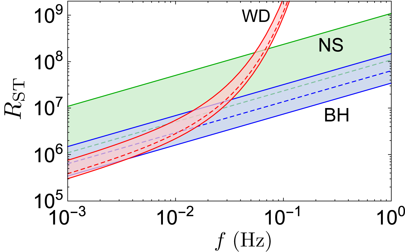
Figure 3: (Color Online). Upper limit on the scalar-to-tensor ratio $R_{\rm ST}$ for each GWB source with uncertainties of merger rates: WD binaries (red), NS binaries (green), and BH binaries (blue). The dashed lines correspond to the intermediate merger rates and the solid lines are the lowest and highest merger rates.

In Fig. 3, the constraints on $R_{\rm ST}$ for each GW source are shown. The upper bound is tighter at lower frequencies, which are at $1\,{\rm mHz}$, $3.9\times 10^{5}$, $1.1\times 10^{6}$, and $6.4\times 10^{5}$ for the intermediate merger rates of WD, NS, and BH binaries, respectively. Although the numerical values appear to be much larger than one, they are the first constraints on $R_{\rm ST}$ obtained in the frequency band from $1\,{\rm mHz}$ to $1\,{\rm Hz}$ in the low-density and weak-gravity region of space, and they connect the physics of GW emission of a source and a screening mechanism in a model-independent way. There have been the constraints at different frequencies from other observations. The observation of the orbital-period derivative from PSR B1913+16 agrees well with predicted values of GR, conservatively, at a level of $1\,\%$ error Weisberg et al. (2010). This fact indicates that the contribution of scalar GWs to the energy loss is less than $1\,\%$, that is, $R_{\rm{ST}}\lesssim 10^{-1}$ at $7.2\times 10^{-5}\,{\rm Hz}$ at the source position of the NS binary. On the other hand, the recent detection of GWs (GW150914) Abbott et al. (2016) gives no constraint on the scalar component, as at least three detectors are needed to break the degeneracy of the polarization modes Nishizawa et al. (2010).

IV Discussion and Conclusion

Comparing to single path pulsar timing measurements, the scintillation measurements have better timing accuracies, and the phase-comparison geometry which naturally removes intrinsic noise from the source. These are the key factors which ensures its ultra precision and enables its application to studying ISM physics, pulsar physics, and our proposal in this paper - testing alternative gravity models.

We have illustrated an example in this proposal: measuring a longitudinal scalar GWB. It is also possible to apply to other tests which do not involve GWs - for example, the spacetime quantum fluctuations Ng and van Dam (1994); Amelino-Camelia (1999) or the holographic noise Hogan (2008). They would contribute distinctive phase noise for photon traveling along different scintillation paths, and hence can be measured by observing anomalous scintillation phase shift or degrading of the interference pattern.