$\boldsymbol{SU(3)_{C}\otimes SU(3)_{L}\otimes U(1)_{X}}$ models in view of the $750$ GeV diphoton signal

Abstract

We analyze the recent diphoton signal reported by ATLAS and CMS collaborations in the context of the $SU(3)_{C}\otimes SU(3)_{L}\otimes U(1)_{X}$ anomaly free models, with a 750 GeV scalar candidate which can decay into two photons. These models may explain the 750GeV signal by means of one loop decays to $\gamma\gamma$ through charged vector and Higgs bosons, as well as top-, bottom- and electron-like exotic particles that arise naturally from the condition of anomaly cancellations of the $SU(3)_{C}\otimes SU(3)_{L}\otimes U(1)_{X}$ models.

I Introduction

The recent excess in the 2015 ATLAS and CMS data with two photons in the final state at invariant mass of about 750 GeV CMS750 ; ATLAS750 has put under observation and testing a large number of models in order to explain it (for a complete list of references see tools ; Ellis ).

Particularly, we are interested in testing the models with gauge symmetry $SU(3)_{C}\otimes SU(3)_{L}\otimes U(1)_{X},$ also called 331 models Georgi-Pais ; Pleitez ; Frampton ; Long ; Pisano . In these models, after imposing some restrictions, as for example the cancellation of anomalies, a free parameter $\beta$ remains and therefore it is not possible to identify a unique version of a 331 model. The $\beta$ parameter determines the fermionic content of the model. For example, for a given representation and $\beta=\sqrt{3}$ there appears exotic quarks and leptons with electric charge $5/3$ and -2 times the proton charge, respectively, while for $\beta=-1/\sqrt{3}$ there appears new quarks of charge $2/3$ and extra neutrinos.

Recently, the diphoton excess analysis in the context of these models has been addressed in references 331diphoton . Here we consider the general case for $\beta=\pm\sqrt{3},$ and $\beta=\pm 1/\sqrt{3}$ and two possible representations Georgi-Pais ; Pleitez ; Frampton taking into account possible interference effects between the new vector and charged Higgs bosons that arise in the 331 models, which can change considerably the production cross section.

Since the 331 models require the three families in order to cancel chiral anomaliesanomalias , these models arise as a possible solution to the generation puzzle. They can also predict the charge quantization for a three family model even when neutrino masses are added Pires . Also, in the framework of supersymmetric 331 models, the breaking chain GUT$\rightarrow 331\rightarrow SM$ is allowed and the model is protected from fast proton decay Martinez2 . In addition, recent versions of the model have addressed the mass hierarchy problem both in the quark and lepton sectors martinez2006 ; Dias ; Dong ; Martinez-Carcamo ; Long-1 ; Valle as well as the dark matter problem Mizukoshi ; Dias2010 ; Alvares2012 ; Cogollo2014 ; Queiroz-Martinez .

However, there are some features that neither SM SM nor the 331 extensions have been able to explain at a cosmological level, such as the formation of large scale structures in the universe Volkas , the origin of the galactic halo Mohapatra , and the observations of gamma ray bursts Wong . On the other hand, the model is purely left-handed, so that it cannot account for the parity breaking. Another point of interest to study in these models is the CP violation, particularly the strong CP violation which might allow us to understand the values of the electric dipole moment of the neutron and electron Pal ; Dias-Pleitez-pires .

This paper is organized as follows. In section 2, we review the main features of the 331 models, their spontaneous symmetry breaking (SSB) scheme, their Higgs potentials as well as the Yukawa Lagrangians with the relevant particle content resulting from the $\beta$ parameter choice. Then, in section 3, we study the diphoton decay in the framework of the 331 models for $\beta=\pm\sqrt{3},$ and $\beta=\pm 1/\sqrt{3}$, finding restrictions for each case consistent with the reported cross section of the 750 GeV signal.

II Description of the model

Although cancellation of anomalies leads to some conditions fourteen , such criterion alone still permits an infinite number of 331 models. In these models, the electric charge is defined in general as a linear combination of the diagonal generators of the group

$$Q=T_{3}+\beta T_{8}+XI,$$ (1)

with $T_{3}=\frac{1}{2}diag(1,-1,0)$ and $T_{8}=\frac{1}{2\sqrt{3}}diag(1,1,-2),$ $I=diag\left(1,1,1\right)$ is the identity matrix and $X$ is the quantum number associated to the $U(1)_{X}$ group. The study of $\beta$ is interesting because it determines the fermion assignment, and more specifically, the electric charges of the extra particle sector. We consider the most popular models for $\beta=\pm\sqrt{3},$ and $\beta=\pm 1/\sqrt{3}\$Georgi-Pais ; Pleitez ; Frampton ; Martinez-Diaz-Ochoa . Here, we assume the following symmetry breaking pattern

$$SU\left(3\right)_{C}\otimes SU\left(3\right)_{L}\otimes U\left(1\right)_{X} \rightarrow SU\left(3\right)_{C}\otimes SU\left(2\right)_{L}\otimes U\left(1\right)_{Y}\rightarrow SU\left(3\right)_{C}\otimes U\left(1\right)_{Q},$$

$$331 \rightarrow 321\rightarrow 31.$$

Although the spontaneous symmetry breaking of the group is possible with less than three scalar triplets, this option does not allow a Peccei-Quinn symmetry in order to face the strong-CP problem Peccei-Dong . So, we use one scalar triplet for the first symmetry breaking and two scalar triplets for the second to give masses to the up and down sectors of the SM (see Table 1). The triplet field $\chi$ only introduce a VEV on the third component for the first transition and induces the masses of the exotic fermionic components. In the second transition pairs of solutions are obtained according to the value of $\beta$. A detailed analysis of such solutions shows that two multiplets are necessary in order to give masses to the quarks of type up and down simultaneously Martinez-Diaz-Ochoa . Therefore, we introduce two triplets$\;\rho$ and $\eta$ in the second transition. In some cases a scalar sextet is introduced to give masses to the neutrinos Pleitez .

Spectrum	$\mathit{SU(3)_{L}\otimes U(1)_{X}}$	$\mathit{Q}$
$\chi=\begin{pmatrix}\chi_{1}^{\mathit{\pm Q_{1}}}\\ \chi_{2}^{\mathit{\pm Q_{2}}}\\ \frac{1}{\sqrt{2}}(\upsilon_{\chi}+\xi_{\chi}\pm i\zeta_{\chi})\end{pmatrix}$	$\left(\mathbf{3},\frac{\beta}{\sqrt{3}}\right)$	$\begin{pmatrix}\pm\left(\frac{1}{2}+\frac{\sqrt{3}\beta}{2}\right)\\ \pm\left(-\frac{1}{2}+\frac{\sqrt{3}\beta}{2}\right)\\ 0\end{pmatrix}$
$\rho=\begin{pmatrix}\rho_{1}^{\pm}\\ \frac{1}{\sqrt{2}}(\upsilon_{\rho}+\xi_{\rho}\pm i\zeta_{\rho})\\ \rho_{3}^{\mathit{\mp Q_{2}}}\end{pmatrix}$	$\left(\mathbf{3},\frac{1}{2}-\frac{\beta}{2\sqrt{3}}\right)$	$\begin{pmatrix}\pm 1\\ 0\\ \mp\left(-\frac{1}{2}+\frac{\sqrt{3}\beta}{2}\right)\end{pmatrix}$
$\eta=\begin{pmatrix}\frac{1}{\sqrt{2}}(\upsilon_{\eta}+\xi_{\eta}\pm i\zeta_{\eta})\\ \eta_{2}^{\mp}\\ \eta_{3}^{\mp\mathit{Q_{1}}}\end{pmatrix}$	$\left(\mathbf{3},-\frac{1}{2}-\frac{\beta}{2\sqrt{3}}\right)$	$\begin{pmatrix}0\\ \mp 1\\ \mp\left(\frac{1}{2}+\frac{\sqrt{3}\beta}{2}\right)\end{pmatrix}$

Table 1: Scalar spectrum for the SSB $331\rightarrow 321\rightarrow 31$. Here $Q_{1}=\frac{1}{2}+\frac{\sqrt{3}\beta}{2}$ and $Q_{2}=-\frac{1}{2}+\frac{\sqrt{3}\beta}{2}$.

.

$\beta$	$V_{\xi_{\chi}}$	$\mathcal{L}_{\xi_{\chi}}^{HVV}$
$\frac{1}{\sqrt{3}}$	$\lambda_{7}\upsilon_{\chi}\xi_{\chi}\eta_{3}^{+}\eta_{3}^{-}$	$\frac{g_{L}m_{K}}{\sqrt{2}}\xi_{\chi}K^{\mu\pm}K_{\mu}^{\mp}$
$-\frac{1}{\sqrt{3}}$	$\lambda_{8}\upsilon_{\chi}\xi_{\chi}\rho_{3}^{+}\rho_{3}^{-}$	$\frac{g_{L}m_{K}}{\sqrt{2}}\xi_{\chi}K^{\mu\pm}K_{\mu}^{\mp}$
$\sqrt{3}$	$\qquad\upsilon_{\chi}\xi_{\chi}\left(\lambda_{7}\eta_{3}^{++}\eta_{3}^{--}+\lambda_{8}\rho_{3}^{+}\rho_{3}^{-}\right)\qquad$	$\frac{g_{L}\xi_{\chi}}{\sqrt{2}}\left(m_{K^{++}}K^{\mu\pm\pm}K_{\mu}^{\mp\mp}+m_{K}K^{\mu\pm}K_{\mu}^{\mp}\right)$
$-\sqrt{3}$	$\upsilon_{\chi}\xi_{\chi}\left(\lambda_{7}\eta_{3}^{+}\eta_{3}^{-}+\lambda_{8}\rho_{3}^{++}\rho_{3}^{--}\right)$	$\qquad\frac{g_{L}\xi_{\chi}}{\sqrt{2}}\left(m_{K^{--}}K^{\mu\mp}K_{\mu}^{\pm}+m_{K}K^{\mu\mp}K_{\mu}^{\pm}\right)\qquad$

Table 2: Relevant bosonic trilinear couplings with $\xi_{\chi}$.

II.1 Bosonic sector

The most general and renormalizable form of the Higgs potential, taking into account all the possible linear combinations among the three triplets forming quadratic, cubic, and quartic products invariant under $SU(3)_{L}\otimes U(1)_{X}$ is given by Martinez-Diaz-Ochoa :

1. For $\beta=\frac{1}{\sqrt{3}}$

   $$V =\mu_{1}^{2}\chi^{i}\chi_{i}+\mu_{2}^{2}\rho^{i}\rho_{i}+\mu_{3}^{2}\eta^{i}\eta_{i}+\mu_{4}^{2}\left(\chi^{i}\rho_{i}+h.c\right)+f\left(\chi_{i}\rho_{j}\eta_{k}\varepsilon^{ijk}+h.c\right)$$

   $$+\lambda_{1}(\chi^{i}\chi_{i})^{2}+\lambda_{2}(\rho^{i}\rho_{i})^{2}+\lambda_{3}(\eta^{i}\eta_{i})^{2}+\lambda_{4}\chi^{i}\chi_{i}\rho^{j}\rho_{j}+\lambda_{5}\chi^{i}\chi_{i}\eta^{j}\eta_{j}$$

   $$+\lambda_{6}\rho^{i}\rho_{i}\eta^{j}\eta_{j}+\lambda_{7}\chi^{i}\eta_{i}\eta^{j}\chi_{j}+\lambda_{8}\chi^{i}\rho_{i}\rho^{j}\chi_{j}+\lambda_{9}\eta^{i}\rho_{i}\rho^{j}\eta_{j}$$

   $$+\lambda_{10}\chi^{i}\chi_{i}\left(\chi^{j}\rho_{j}+h.c.\right)+\lambda_{11}\rho^{i}\rho_{i}\left(\rho^{j}\chi_{j}+h.c.\right)+\lambda_{12}\eta^{i}\eta_{i}\left(\chi^{j}\rho_{j}+h.c.\right)$$

   $$+\lambda_{13}\left(\chi^{i}\rho_{i}\chi^{j}\rho_{j}+h.c.\right)+\lambda_{14}\left(\eta^{i}\chi_{i}\rho^{j}\eta_{j}+h.c.\right).$$ (2)

2. For $\beta=-\frac{1}{\sqrt{3}}$

   $$V =\mu_{1}^{2}\chi^{i}\chi_{i}+\mu_{2}^{2}\rho^{i}\rho_{i}+\mu_{3}^{2}\eta^{i}\eta_{i}+\mu_{4}^{2}\left(\chi^{i}\eta_{i}+h.c\right)+f\left(\chi_{i}\rho_{j}\eta_{k}\varepsilon^{ijk}+h.c\right)$$

   $$+\lambda_{1}(\chi^{i}\chi_{i})^{2}+\lambda_{2}(\rho^{i}\rho_{i})^{2}+\lambda_{3}(\eta^{i}\eta_{i})^{2}+\lambda_{4}\chi^{i}\chi_{i}\rho^{j}\rho_{j}+\lambda_{5}\chi^{i}\chi_{i}\eta^{j}\eta_{j}$$

   $$+\lambda_{6}\rho^{i}\rho_{i}\eta^{j}\eta_{j}+\lambda_{7}\chi^{i}\eta_{i}\eta^{j}\chi_{j}+\lambda_{8}\chi^{i}\rho_{i}\rho^{j}\chi_{j}+\lambda_{9}\eta^{i}\rho_{i}\rho^{j}\eta_{j}$$

   $$+\lambda_{10}\chi^{i}\chi_{i}\left(\chi^{j}\eta_{j}+h.c.\right)+\lambda_{11}\eta^{i}\eta_{i}\left(\eta^{j}\chi_{j}+h.c.\right)+\lambda_{12}\rho^{i}\rho_{i}\left(\chi^{j}\eta_{j}+h.c.\right)$$

   $$+\lambda_{13}\left(\chi^{i}\eta_{i}\chi^{j}\eta_{j}+h.c.\right)+\lambda_{14}\left(\rho^{i}\chi_{i}\eta^{j}\rho_{j}+h.c.\right).$$ (3)

3. For $\beta=\sqrt{3}$

   $$V =\mu_{1}^{2}\chi^{i}\chi_{i}+\mu_{2}^{2}\rho^{i}\rho_{i}+\mu_{3}^{2}\eta^{i}\eta_{i}+f\left(\chi_{i}\rho_{j}\eta_{k}\varepsilon^{ijk}+h.c\right)+\lambda_{1}(\chi^{i}\chi_{i})^{2}+\lambda_{2}(\rho^{i}\rho_{i})^{2}$$

   $$+\lambda_{3}(\eta^{i}\eta_{i})^{2}+\lambda_{4}\chi^{i}\chi_{i}\rho^{j}\rho_{j}+\lambda_{5}\chi^{i}\chi_{i}\eta^{j}\eta_{j}+\lambda_{6}\rho^{i}\rho_{i}\eta^{j}\eta_{j}+\lambda_{7}\chi^{i}\eta_{i}\eta^{j}\chi_{j}$$

   $$+\lambda_{8}\chi^{i}\rho_{i}\rho^{j}\chi_{j}+\lambda_{9}\eta^{i}\rho_{i}\rho^{j}\eta_{j}+\lambda_{10}\left(\rho^{i}\chi_{i}\rho^{j}\eta_{j}+h.c.\right).$$ (4)

4. For $\beta=-\sqrt{3}$

   $$V =\mu_{1}^{2}\chi^{i}\chi_{i}+\mu_{2}^{2}\rho^{i}\rho_{i}+\mu_{3}^{2}\eta^{i}\eta_{i}+f\left(\chi_{i}\rho_{j}\eta_{k}\varepsilon^{ijk}+h.c\right)+\lambda_{1}(\chi^{i}\chi_{i})^{2}+\lambda_{2}(\rho^{i}\rho_{i})^{2}$$

   $$+\lambda_{3}(\eta^{i}\eta_{i})^{2}+\lambda_{4}\chi^{i}\chi_{i}\rho^{j}\rho_{j}+\lambda_{5}\chi^{i}\chi_{i}\eta^{j}\eta_{j}+\lambda_{6}\rho^{i}\rho_{i}\eta^{j}\eta_{j}+\lambda_{7}\chi^{i}\eta_{i}\eta^{j}\chi_{j}$$

   $$+\lambda_{8}\chi^{i}\rho_{i}\rho^{j}\chi_{j}+\lambda_{9}\eta^{i}\rho_{i}\rho^{j}\eta_{j}+\lambda_{10}\left(\eta^{i}\chi_{i}\eta^{j}\rho_{j}+h.c.\right).$$ (5)

The rotation matrices to mass eigenvectors will have the standard form

$$\left(\begin{array}[]{c}\eta_{2}^{\pm}\\ \rho_{1}^{\pm}\end{array}\right)=\left(\begin{array}[]{cc}C_{\beta}&S_{\beta}\\ -S_{\beta}&C_{\beta}\end{array}\right)\left(\begin{array}[]{c}G^{\pm}\\ H^{\pm}\end{array}\right),$$ (6)

$$\left(\begin{array}[]{c}\xi_{\rho}\\ \xi_{\eta}\\ \xi_{\chi}\end{array}\right)=\left(\begin{array}[]{ccc}C_{\alpha}&S_{\alpha}&0\\ -S_{\alpha}&C_{\alpha}&0\\ 0&0&1\end{array}\right)\left(\begin{array}[]{c}h\\ H\\ H_{3}\end{array}\right).$$ (7)

We take the real component $\xi_{\chi}$ from the field $\chi$ as our 750 GeV signal candidate, corresponding to one of the residual physical particles after the $SU\left(3\right)_{L}\otimes U\left(1\right)_{X}$ symmetry breaking, while the imaginary component $\zeta_{\chi}$ corresponds to the would-be Goldstone boson that become into the longitudinal component of a $Z^{\prime}$ gauge boson. So, after rotation to mass eigenvectors according to Eqs.(6-7), we obtain all the interactions of $\xi_{\chi}$ with the scalar matter in the framework of an effective Two Higgs Doublet Model (2HDM) in the low energy limit, where both electroweak triplets $\rho$ and $\eta$ are decomposed into two hypercharge-one $SU(2)_{L}$ doublets plus charged and neutral singlets. In particular, the masses of the extra neutral, pseudoscalar and charged Higgs bosons $H$, $A$ and $H^{\pm}$, respectively, are nearly degenerated and at the TeV scale, as shown in Martinez-Diaz-Ochoa . So, the decay of $\xi_{\chi}$ into these Higgs bosons are kinematically forbidden. Explicitly, the couplings with the resulting charged Higgs boson $H^{\pm}$ of the 2HDM are given by

$$V_{\xi_{\chi}}^{\mathrm{2HDM}} =\upsilon_{\chi}\xi_{\chi}\left[\left(\lambda_{4}C_{\beta}^{2}+\lambda_{5}S_{\beta}^{2}\right)H^{+}H^{-}+\frac{1}{2}\left(\lambda_{4}C_{\alpha}^{2}+\lambda_{5}S_{\alpha}^{2}\right)h^{2}\right.$$

$$\left.+\frac{1}{2}\left(\lambda_{4}S_{\alpha}^{2}+\lambda_{5}C_{\alpha}^{2}\right)H^{2}+\left(\lambda_{4}-\lambda_{5}\right)C_{\alpha}S_{\alpha}hH\right].$$ (8)

For the 331 models, in the limit $\upsilon_{\chi}^{2}>>\upsilon_{\rho}^{2},\upsilon_{\eta}^{2}$ we obtain the relation $\alpha\approx\beta\pm\frac{\pi}{2}$ Martinez-Diaz-Ochoa allowing us to simplify the previous expression to

$$V_{\xi_{\chi}}^{\mathrm{2HDM}} =\upsilon_{\chi}\xi_{\chi}\left[\lambda\left(H^{+}H^{-}+\frac{h^{2}+H^{2}}{2}\right)+\left(\lambda_{4}-\lambda_{5}\right)C_{\alpha}S_{\alpha}hH\right]$$ (9)

where we have defined $\lambda\equiv\lambda_{4}S_{\alpha}^{2}+\lambda_{5}C_{\alpha}^{2}$. Also, as a particular case, if we had set $\lambda_{4}=\lambda_{5}$ in Eq.(8), we would have obtained the same coupling for the decay $\xi_{\chi}\rightarrow hh$ and $\xi_{\chi}\rightarrow H^{+}H^{-}$ independently on the mixing angles. In this way, since the decay $\xi_{\chi}\rightarrow hh$ is strongly constrained by ATLAS and CMS at 95%CL Ellis , the coupling between $\xi_{\chi}$ and $H^{\pm}$ is also suppressed, thus the charged Higgs boson $H^{\pm}$ will not contribute to the diphoton decay.

On the other hand, the relevant trilinear couplings with the extra vector bosons $K^{\pm Q_{1}}$ and $K^{\pm Q_{2}}$ are given by Martinez-Diaz-Ochoa

$$\mathcal{L}_{\xi_{\chi}}^{HVV}=\frac{g_{L}\xi_{\chi}}{\sqrt{2}}\left(m_{K^{Q_{1}}}K^{\mu\pm Q_{1}}K_{\mu}^{\mp Q_{1}}+m_{K^{Q_{2}}}K^{\mu\pm Q_{2}}K_{\mu}^{\mp Q_{2}}\right).$$ (10)

where $g_{L}$ is the $SU(2)_{L}$ coupling constant. Taking into account all the above conditions and after the $SU\left(3\right)_{L}\otimes U\left(1\right)_{X}$ symmetry breaking by $\upsilon_{\chi}$, we obtain the relevant trilinear bosonic couplings with the third components of the triplets which correspond to singlets fields under the SM. According to the $\beta$ value, these singlet fields can be charged or doubly charged, contributing to the diphoton decay according to the Feynman rules in Table 2. In the loops we will refer to these fields as $h^{\pm}$ and $h^{\pm\pm}$, respectively.

II.2 Fermionic sector

The fermions exhibit the following general structure of transformations under the chiral group $SU(3)_{L}\otimes U(1)_{X}$

$$\psi_{L} = \left\{\begin{array}[]{c}q_{L}:\left(\mathbf{3,}X_{q}^{L}\right)=\left(\mathbf{2,}X_{q}^{L}\right)\oplus\left(\mathbf{1,}X_{q}^{L}\right),\\ \ell_{L}:\left(\mathbf{3,}X_{\ell}^{L}\right)=\left(\mathbf{2,}X_{\ell}^{L}\right)\oplus\left(\mathbf{1,}X_{\ell}^{L}\right),\end{array}\right.$$ (13)

$$\psi_{L}^{\ast} = \left\{\begin{array}[]{c}q_{L}^{\ast}:\left(\mathbf{3}^{\ast}\mathbf{,-}X_{q}^{L}\right)=\left(\mathbf{2}^{\ast}\mathbf{,-}X_{q}^{L}\right)\oplus\left(\mathbf{1,-}X_{q}^{L}\right)\mathbf{,}\\ \ell_{L}^{\ast}:\left(\mathbf{3}^{\ast}\mathbf{,-}X_{\ell}^{L}\right)=\left(\mathbf{2}^{\ast}\mathbf{,-}X_{\ell}^{L}\right)\oplus\left(\mathbf{1,-}X_{\ell}^{L}\right),\end{array}\right.$$ (16)

$$\psi_{R} = \left\{\begin{array}[]{c}q_{R}:\left(\mathbf{1,}X_{q}^{R}\right),\\ \ell_{R}:\left(\mathbf{1,}X_{\ell}^{R}\right),\end{array}\right.$$ (19)

where the quarks $q$ can be either color triplets (3) or antitriplets ($\boldsymbol{3^{*}}$) according to the representation choice and the leptons $\ell$ are color singlets (1). The second equality corresponds to the branching rules $SU(2)_{L}\subset SU(3)_{L}$. The possibilities $\mathbf{3}$ and $\boldsymbol{3^{*}}$ are included in both the color and flavor sector since the same number of fermion triplets and antitriplets must be present in order to cancel anomalies doff and the quantum number $X$, associated with the parameter $\beta$, will take specific values according to the representations of $SU(3)_{L}$ and the anomalies cancellation. In this way, there are two possible representations for the 331 models that are mutually conjugated, that we call models A and A*. The difference between the two models is to change $\beta$ in model A by $-\beta$ in model A* (Tables 3-4). Henceforth we will use the model A in order to evaluate the production cross section.

Model	Spectrum	$SU\left(3\right)_{L}\otimes U\left(1\right)_{X}$	$\mathit{Q}$
A	$q_{L}^{3}=\left(\begin{array}[]{c}U^{3}\\ D^{3}\\ T^{3}(J^{3})\end{array}\right)_{L}$	$\left(\mathbf{3},\frac{1}{6}-\frac{\beta}{2\sqrt{3}}\right)$	$\left(\begin{array}[]{c}\frac{2}{3}\\ -\frac{1}{3}\\ \frac{1}{6}-\frac{\sqrt{3}\beta}{2}\end{array}\right)$
	$U_{R}^{3}$,$D_{R}^{3}$,$T_{R}^{3}$,$(J_{R}^{3})$	$\qquad\left(\mathbf{1},\frac{2}{3}\right)$,$\left(\mathbf{1},-\frac{1}{3}\right)$,$\left(\mathbf{1},\frac{1}{6}-\frac{\sqrt{3}\beta}{2}\right)\qquad$	$\frac{2}{3}$,$-\frac{1}{3}$,$\frac{1}{6}-\frac{\sqrt{3}\beta}{2}$
	$q_{L}^{1,2}=\left(\begin{array}[]{c}D^{1,2}\\ -U^{1,2}\\ J^{1,2}(T^{1,2})\end{array}\right)_{L}$	$\left(\boldsymbol{3^{*}},\frac{1}{6}+\frac{\beta}{2\sqrt{3}}\right)$	$\left(\begin{array}[]{c}-\frac{1}{3}\\ \frac{2}{3}\\ \frac{1}{6}-\frac{\sqrt{3}\beta}{2}\end{array}\right)$
	$D_{R}^{1,2}$,$U_{R}^{1,2}$,$J_{R}^{1,2}(T^{1,2})$	$\qquad\left(\mathbf{1},-\frac{1}{3}\right)$,$\left(\mathbf{1},\frac{2}{3}\right)$,$\left(\mathbf{1},\frac{1}{6}+\frac{\sqrt{3}\beta}{2}\right)\qquad$	$-\frac{1}{3}$,$\frac{2}{3}$,$\frac{1}{6}+\frac{\sqrt{3}\beta}{2}$
	$\ell_{L}^{(n)}=\left(\begin{array}[]{c}\nu^{n}\\ e^{n}\\ E^{n}\end{array}\right)_{L}$	$\left(\mathbf{3},-\frac{1}{2}-\frac{\beta}{2\sqrt{3}}\right)$	$\left(\begin{array}[]{c}0\\ -1\\ -\frac{1}{2}-\frac{\sqrt{3}\beta}{2}\end{array}\right)$
	$\nu_{R}^{n}$,$\mathit{e_{R}^{n}}$,$\mathit{E_{R}^{n}}$	$\qquad\left(\mathbf{1},0\right)$,$\left(\mathbf{1},-1\right)$,$\left(\mathbf{1},-\frac{1}{2}-\frac{\sqrt{3}\beta}{2}\right)\qquad$	$0$,$-1$,$-\frac{1}{2}-\frac{\sqrt{3}\beta}{2}$
A*
	$q_{L}^{3}=\left(\begin{array}[]{c}D^{3}\\ -U^{3}\\ J^{3}(T^{3})\end{array}\right)_{L}$	$\left(\boldsymbol{3^{*}},\frac{1}{6}+\frac{\beta}{2\sqrt{3}}\right)$	$\left(\begin{array}[]{c}-\frac{1}{3}\\ \frac{2}{3}\\ \frac{1}{6}+\frac{\sqrt{3}\beta}{2}\end{array}\right)$
	$D_{R}^{3}$,$U_{R}^{3}$,$J_{R}^{3}$$(T_{R}^{3})$	$\qquad\left(\mathbf{1},-\frac{1}{3}\right)$,$\left(\mathbf{1},\frac{2}{3}\right)$,$\left(\mathbf{1},\frac{1}{6}+\frac{\sqrt{3}\beta}{2}\right)\qquad$	$-\frac{1}{3}$,$\frac{2}{3}$,$\frac{1}{6}+\frac{\sqrt{3}\beta}{2}$
	$q_{L}^{1,2}=\left(\begin{array}[]{c}U^{1,2}\\ D^{1,2}\\ T^{1,2}(J^{1,2})\end{array}\right)_{L}$	$\left(\mathbf{3},\frac{1}{6}-\frac{\beta}{2\sqrt{3}}\right)$	$\left(\begin{array}[]{c}\frac{2}{3}\\ -\frac{1}{3}\\ \frac{1}{6}+\frac{\sqrt{3}\beta}{2}\end{array}\right)$
	$U_{R}^{1,2}$,$D_{R}^{1,2}$,$T^{1,2}(J_{R}^{1,2})$	$\qquad\left(\mathbf{1},\frac{2}{3}\right)$,$\left(\mathbf{1},-\frac{1}{3}\right)$,$\left(\mathbf{1},\frac{1}{6}-\frac{\sqrt{3}\beta}{2}\right)\qquad$	$\frac{2}{3}$,$-\frac{1}{3}$,$\frac{1}{6}-\frac{\sqrt{3}\beta}{2}$
	$\ell_{L}^{(n)}=\left(\begin{array}[]{c}e^{n}\\ -\nu^{n}\\ E^{n}\end{array}\right)_{L}$	$\left(\boldsymbol{3^{*}}-\frac{1}{2}+\frac{\beta}{2\sqrt{3}}\right)$	$\left(\begin{array}[]{c}-1\\ 0\\ -\frac{1}{2}+\frac{\sqrt{3}\beta}{2}\end{array}\right)$
	$\mathit{e_{R}^{n}}$,$\nu_{R}^{n}$,$\mathit{E_{R}^{n}}$	$\qquad\left(\mathbf{1},-1\right)$,$\left(\mathbf{1},0\right)$,$\left(\mathbf{1},-\frac{1}{2}+\frac{\sqrt{3}\beta}{2}\right)\qquad$	$-1$,$0$,$-\frac{1}{2}+\frac{\sqrt{3}\beta}{2}$

Table 3: Particle content for the fermionic sector with $n=1,2,3$. The choice of $T$ or $J$ in the quark triplets depends on the value of $\beta$.

	Fermions in the loop		$Q$
$\beta$	Model A	Model A*	Model A	Model A*
$\frac{1}{\sqrt{3}}$	$\qquad T^{m}$, $J$, $E^{-}\qquad$	$T$, $J^{m}$	$\frac{2}{3}$, $-\frac{1}{3}$,$-1$	$\frac{2}{3}$, $-\frac{1}{3}$
$-\frac{1}{\sqrt{3}}$	$T$, $J^{m}$	$\qquad T^{m}$, $J$, $E^{-}\qquad$	$\frac{2}{3}$, $-\frac{1}{3}$	$\frac{2}{3}$, $-\frac{1}{3}$,$-1$
$\sqrt{3}$	$T^{m}$, $J$, $E^{--}$	$T$, $J^{m}$, $E^{+}$	$\qquad\frac{5}{3}$, $-\frac{4}{3}$, $-2\qquad$	$\frac{2}{3}$, $-\frac{4}{3}$, $+1$
$-\sqrt{3}$	$T$, $J^{m}$, $E^{+}$	$T^{m}$, $J$, $E^{--}$	$\frac{2}{3}$, $-\frac{4}{3}$, $+1$	$\qquad\frac{5}{3}$, $-\frac{4}{3}$, $-2\qquad$

Table 4: Fermions in the loop for every choice of $\beta$. Here $m=1,\,2$.

Regardless the fermionic content of the model, the $\beta$ parameter and the representation choice, the most general, renormalizable, and $SU\left(3\right)_{C}\otimes SU\left(3\right)_{L}\otimes U\left(1\right)_{X}$ invariant Yukawa Lagrangian for quarks is given by

$$-\mathcal{L}_{Y}^{q} = \sum_{m=1}^{2}\overline{q_{L}^{3}}\left(h_{U_{R}^{3}}^{3\eta}U_{R}^{3}\eta+h_{D_{R}^{3}}^{3\rho}D_{R}^{3}\rho+h_{J_{R}^{3}}^{3\chi}J_{R}^{3}\chi+h_{U_{R}^{m}}^{3\eta}U_{R}^{3}\eta+h_{D_{R}^{m}}^{3\rho}D_{R}^{m}\rho\right)$$ (20)

$$+ \sum_{m,m\text{\textasciiacute}=1}^{2}\overline{q_{L}^{m}}\left(h_{D_{R}^{3}}^{m\eta}D_{R}^{3}\eta+h_{U_{R}^{3}}^{m\rho}U_{R}^{3}\rho+h_{D_{R}^{m\text{\textasciiacute}}}^{m\eta}D_{R}^{m\text{\textasciiacute}}\eta+h_{U_{R}^{m\text{\textasciiacute}}}^{m\rho}U_{R}^{m\text{\textasciiacute}}\rho+h_{J_{R}^{m\text{\textasciiacute}}}^{m\chi}J_{R}^{m\text{\textasciiacute}}\chi\right)$$

$$+ \mathcal{L}_{\pm 1/\sqrt{3}}^{q}+h.c.$$

where $\mathcal{L}_{\pm 1/\sqrt{3}}^{q}$ contains mixing terms between the SM light quarks and the exotic quarks $T$ and $J$ given by

$$\mathcal{L}_{1/\sqrt{3}}^{q}= \sum_{m=1}^{2}\overline{q_{L}^{3}}\left(h_{D_{R}^{3}}^{3\chi}D_{R}^{3}\chi+h_{J_{R}^{3}}^{3\rho}J_{R}^{3}\rho+h_{D_{R}^{m}}^{3\chi}D_{R}^{m}\chi+h_{J_{R}^{m}}^{3\eta}J_{R}^{m}\eta\right)$$

$$+ \sum_{m,m\text{\textasciiacute}=1}^{2}\overline{q_{L}^{m}}\left(h_{U_{R}^{3}}^{m\chi}U_{R}^{3}\chi+h_{J_{R}^{3}}^{m\eta}J_{R}^{3}\eta+h_{U_{R}^{m\text{\textasciiacute}}}^{m\chi}U_{R}^{m\text{\textasciiacute}}\chi+h_{J_{R}^{m\text{\textasciiacute}}}^{m\rho}J_{R}^{m\text{\textasciiacute}}\rho\right)+h.c.$$ (21)

$$\mathcal{L}_{-1/\sqrt{3}}^{q}= \sum_{m=1}^{2}\overline{q_{L}^{3}}\left(h_{U_{R}^{3}}^{3\chi}U_{R}^{3}\chi+h_{J_{R}^{3}}^{3\eta}J_{R}^{3}\eta+h_{U_{R}^{m}}^{3\chi}U_{R}^{m}\chi+h_{J_{R}^{m}}^{3\rho}J_{R}^{m}\rho\right)$$

$$+ \sum_{m,m\text{\textasciiacute}=1}^{2}\overline{q_{L}^{m}}\left(h_{D_{R}^{3}}^{m\chi}D_{R}^{3}\chi+h_{J_{R}^{3}}^{m\rho}J_{R}^{3}\rho+h_{D_{R}^{m\text{\textasciiacute}}}^{m\chi}D_{R}^{m\text{\textasciiacute}}\chi+h_{J_{R}^{m\text{\textasciiacute}}}^{m\eta}J_{R}^{m\text{\textasciiacute}}\eta\right)+h.c.$$ (22)

Similarly, for the lepton sector we have

$$-\mathcal{L}_{Y}^{l} = \sum_{n,n^{\prime}=1}^{3}\overline{l_{L}^{n}}\left(h_{\nu_{R}^{n^{\prime}}}^{n\eta}\nu_{R}^{n^{\prime}}\eta+h_{e_{R}^{n^{\prime}}}^{n\rho}e_{R}^{n^{\prime}}\rho+h_{E_{R}^{n^{\prime}}}^{n^{\prime}\chi}E_{R}^{n^{\prime}}\chi\right)$$ (23)

$$+ \mathcal{L}_{\pm 1/\sqrt{3}}^{l}+\mathcal{L}_{-\sqrt{3}}^{l}+h.c.$$

with the mixing terms

$$\mathcal{L}_{1/\sqrt{3}}^{l}=\sum_{n=1}^{3}\overline{l_{L}^{n}}\left(h_{e_{R}^{n}}^{n\chi}e_{R}^{n}\chi+h_{E_{R}^{n}}^{n\rho}E_{R}^{n}\rho\right),$$ (24)

$$\mathcal{L}_{-1/\sqrt{3}}^{l}=\sum_{n=1}^{3}\overline{l_{L}^{n}}\left(h_{\nu_{R}^{n}}^{n\chi}\nu_{R}^{n}\chi+h_{E_{R}^{n}}^{n\eta}E_{R}^{n}\eta\right)+\frac{1}{2}\sum_{n,n^{\prime}=1}^{3}\overline{l_{L}^{in}}\left(l_{L}^{jn\text{\textasciiacute}}\right)^{c}(h_{\rho}\rho_{k})\epsilon^{ijk},$$ (25)

$$\mathcal{L}_{-\sqrt{3}}^{l}=\frac{1}{2}\sum_{n,n^{\prime}=1}^{3}\overline{l_{L}^{in}}\left(l_{L}^{jn\text{\textasciiacute}}\right)^{c}(h_{\eta}\eta_{k})\epsilon^{ijk}.$$ (26)

From the Yukawa Lagrangians in Eqs. (20-23) we obtain the relevant couplings of the $\xi_{\chi}$ component of the scalar triplet $\chi$ with the new quarks $T$ and $J$ (Table 4).

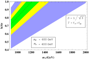
(a)

      

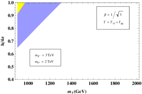
(b)

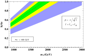
(c)

      

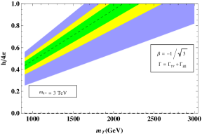
(d)

Figure 1: Contours of the production cross-section $\sigma(pp\to\xi_{\chi}\to\gamma\gamma)$ in femtobarns for $\beta=\pm 1/\sqrt{3}$. The dashed line corresponds to the central value at 6 fb, and the shaded bands corresponds to regions at 68.3% (green), 95.5% (yellow) and 99.7% (light blue) C.L. exclusion limits from ATLAS and CMS combined data.

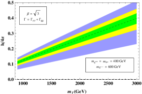
(a)

      

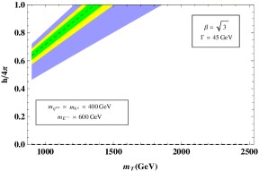
(b)

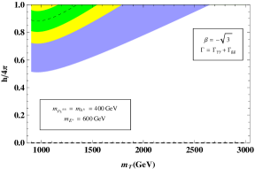
(c)

      

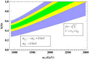
(d)

Figure 2: Contours of the production cross-section $\sigma(pp\to\xi_{\chi}\to\gamma\gamma)$ in femtobarns for $\beta=\pm\sqrt{3}$. The dashed line corresponds to the central value at 6 fb, and the shaded bands corresponds to regions at 68.3% (green), 95.5% (yellow) and 99.7% (light blue) C.L. exclusion limits from ATLAS and CMS combined data.

III Diphoton decay

We will use two approximations for the decay width: first we assume one loop contributions only from diphotons and gluons, $\Gamma=\Gamma_{\gamma\gamma}+\Gamma_{gg}$ . Second we take the width given by the experimentally reported value $\Gamma=45$ GeV from the ATLAS Collaboration. Following Gunion the decay rates of the $\xi_{\chi}$ particle to $\gamma\gamma$ and $gg$ are

$$\Gamma(\xi_{\chi}\to\gamma\gamma) = \frac{\alpha^{2}h^{2}m_{\xi_{\chi}}^{3}}{512\pi^{3}m_{T}^{2}}\big{|}\sum_{i}N_{ci}Q_{i}^{2}F_{i}\big{|}^{2},$$ (27)

$$\Gamma(\xi_{\chi}\to gg) = \frac{\alpha_{s}^{2}h^{2}m_{\xi_{\chi}}^{3}}{64\pi^{3}m_{T}^{2}}\big{|}\sum_{i}F_{i}\big{|}^{2}$$ (28)

where $h$ is the Yukawa coupling of the exotic quarks, $m_{T}$ is the mass of the exotic quarks (assuming the same Yukawa couplings and masses for simplicity, $m_{T}=m_{J}$), $m_{\xi_{\chi}}$ is the mass of the scalar candidate, $N_{ci}Q_{i}^{2}$ is the color multiplicity times the square electric charge and

$$F_{i}(\tau_{i})=\begin{cases}2+3\tau_{i}+3\tau_{i}(2-\tau_{i})f(\tau_{i})&i=1\\ -2\tau_{i}\left[1+(1-\tau_{i})f(\tau_{i})\right]&i=1/2\\ \frac{1}{2}\tau_{i}\left[1-\tau_{i}f(\tau_{i_{i}})\right]&i=0\end{cases}$$ (29)

are spin dependent functions for the loop factor. For $\tau_{i}>1$ the function $f(\tau_{i})$ is $f(\tau_{i})=\left[\arcsin\left(\frac{1}{\sqrt{\tau_{i}}}\right)\right]^{2}$ with $\tau_{i}=4m_{i}^{2}/m_{\xi_{\chi}}^{2}$ from where the masses of the particles into the loop are $m_{i}>375$ GeV . The total cross section $\sigma(pp\to\xi_{\chi}\to\gamma\gamma)$ in the narrow width approximation is given by

$$\sigma(pp\to\xi_{\chi}\to\gamma\gamma)=\frac{C_{gg}\Gamma(\xi_{\chi}\to gg)\Gamma(\xi_{\chi}\to\gamma\gamma)}{s\>m_{\xi_{\chi}}\Gamma}$$ (30)

where $C_{gg}$ is the dimensionless partonic integral computed for a resonance $m_{\xi_{\chi}}=750$ GeV evaluated at the scale $\mu=m_{\xi_{\chi}}$ and center of mass energy $\sqrt{s}=13\,\mathrm{TeV}$, $C_{gg}=2137$ Cgg .

Here, we have taken $m_{K^{\pm Q_{1}}}=m_{K^{\pm Q_{2}}}\sim 3$ TeV according to ATLAS and CMS Collaborations searches CMS ATLAS W' mass . However, for $m_{K^{\pm Q_{1}}}=m_{K^{\pm Q_{2}}}\sim 3$ TeV the associated form factor $F_{1}$ reaches its asymptotic value, and the cross section dependence on $m_{K^{\pm Q_{1}}}$ and $m_{K^{\pm Q_{2}}}$ is not appreciable. So, the production cross section will depend only on the Yukawa coupling $h$, the mass of the quarks $m_{T}$ and on the exotic charged lepton masses $m_{E^{-}}$, $m_{E^{--}}$. From the lower bound reported by the ATLAS Collaboration searches on exotic heavy charged leptons lepton masses we set $m_{E^{-}}=m_{E^{--}}\sim 600$ GeV. For the analysis we take the combined results for the cross section from CMS and ATLAS, $\sigma(pp\to\xi_{\chi}\to\gamma\gamma)=(2-8)\>\mathrm{fb}$ tools .

Taking into account all the above conditions, we display in Figs.1-2 contour plots of the production cross-section $\sigma(pp\to\xi_{\chi}\to\gamma\gamma)$ as function of the Yukawa coupling normalized as $h/4\pi$ and on the top-like quark mass $m_{T}$. The lower bound of 900 GeV for $m_{T}$ corresponds to the reported value in recent searches on top- and bottom-like heavy quarks from ATLAS and CMS Collaborations quark masses and the upper bound of 3 TeV corresponds to the asymptotic value obtained from the fermionic form factor $F_{1/2}$. We have also taken for simplicity $m_{h^{\pm}}\equiv m_{\eta_{3}^{\pm}}=m_{\rho_{3}^{\pm}}=400$ GeV and $m_{\eta_{3}^{\pm\pm}}=m_{\rho_{3}^{\pm\pm}}=400$ GeV which corresponds to the lowest bound from charged Higgs boson searches reported by ATLAS and CMS charged higgs while for the upper bound we have used $m_{h^{\pm}}=m_{\eta_{3}^{\pm\pm}}=m_{\rho_{3}^{\pm\pm}}=3$ TeV associated to the asymptotic value obtained from the bosonic form factor $F_{0}$.

In general, from Figs.1-2 we can observe that the Yukawa couplings for the smallest masses and positive values of $\beta$ are larger than for the masses in the asymptotic values. Conversely, for negative values of $\beta$ the larger the mass parameters, the smaller the Yukawa couplings. Furthermore, every model exhibits an allowed region for the diphoton production cross section when $\Gamma=\Gamma_{\gamma\gamma}+\Gamma_{gg}$. In contrast, for the case $\Gamma=45$ GeV there are allowed regions only for $\beta=\sqrt{3}$.

Particularly, for $\beta=1/\sqrt{3}(-1/\sqrt{3})$ and mass lower bounds choices, the model is excluded for Yukawa couplings $h/4\pi<0.4\,(0.3)$ and masses of the exotic quarks $m_{T}>2\,\mathrm{TeV}\,(3\,\mathrm{TeV})$. On the other hand, for the asymptotic values, the model is excluded for Yukawa couplings $h/4\pi<0.7\,(0.3)$ and masses of the exotic quarks $m_{T}>1.3\,\mathrm{TeV}\,(3\,\mathrm{TeV})$. Also, for $\beta=\sqrt{3}(-\sqrt{3})$ and lower bound choices, the model is excluded for Yukawa couplings $h/4\pi<0.1\,(0.6)$ and masses of the exotic quarks $m_{T}>2.5\,\mathrm{TeV}\,(5\,\mathrm{TeV})$. For $\beta=\sqrt{3}$ and $\Gamma=45$ GeV, the model is excluded for Yukawa couplings $h/4\pi<0.5$ and masses of the exotic quarks $m_{T}>1.8\,\mathrm{TeV}$. Since the exotic quarks and charged Higgs bosons have electric charge $5/3$ and -2 respectively, the model for $\beta=\sqrt{3}$ exhibits the smallest Yukawa coupling values (Fig. 3).

III.1 Interference effects

From Eq.(29) we can see a sign difference between the fermionic and bosonic contributions into the loop for the diphoton decay. This difference is responsible for interference effects that can affect considerably the production cross section as shown in Figs 4-7.

We show in Figs. 4, 5, 6 and 7 the interference effects from the different contributions for the 331 model for $\beta=1/\sqrt{3},\,-1/\sqrt{3},\,\sqrt{3}$ and $-\sqrt{3}$ respectively. In general, for all $\beta$ values we can observe the largest interference effects when we only take into account the vector bosons $K$ (red dotted lines) and the smallest interference effects arise from the charged Higgs bosons $h^{\pm}$ or $h^{\pm\pm}$ (black dashed lines). Also, we can see that for the contribution coming only from fermions (green line), we obtain that the Yukawa couplings take smaller values than when we take into account all the particles into the loop (blue dot-dashed lines) except for $\beta=-1/\sqrt{3}$.

Particularly, for model A and $\beta=1/\sqrt{3}$ (Fig 4) taking into account only the fermionic contributions (green line) we obtain allowed regions for $m_{T}$ in agreement with LHC limits. Also, if we add the charged Higgs boson into the loop (black dashed line) we obtain allowed regions with $m_{T}>900$ GeV . In contrast, if we take into account the contribution of the gauge boson $K^{\pm}$, it produces a strong effect on the production cross section (red dotted line) excluding the model for the allowed values of $m_{T}>900$ GeV. However, if we add all the contributions into the loop (blue dot-dashed line) there appears an allowed region for $m_{T}>900$ GeV.

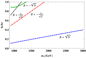
(a)

      

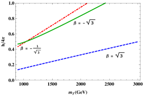
(b)

Figure 3: Contours of the production cross-section $\sigma(pp\to\xi_{\chi}\to\gamma\gamma)$ in femtobarns for the best fit value of 6 fb for (a) mass lower bounds values reported by LHC and (b) asymptotic mass values coming from the form factors $F_{i}$ with $i=0,\,1/2,\,1$.

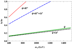
(a)

      

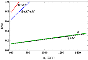
(b)

Figure 4: Contours of the production cross-section $\sigma(pp\to\xi_{\chi}\to\gamma\gamma)$ in femtobarns for the best fit value of 6 fb for (a) mass lower bounds values reported by LHC and (b) asymptotic mass values coming from the form factors $F_{i}$ with $i=0,\,1/2,\,1$. Here $\beta=1/\sqrt{3}$ for model A with $\psi=(T^{m},\,J,\,E^{-})$. The green (thick), black (dashed), blue (dot-dashed) and red (dotted) lines correspond to the contributions coming from $\psi$, $\psi+h^{\pm}$, $\psi+K^{\pm}+h^{\pm}$ and $\psi+K^{\pm}$ respectively.

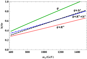
(a)

      

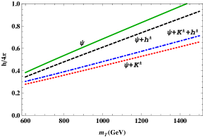
(b)

Figure 5: Contours of the production cross-section $\sigma(pp\to\xi_{\chi}\to\gamma\gamma)$ in femtobarns for the best fit value of 6 fb for (a) mass lower bounds values reported by LHC and (b) asymptotic mass values coming from the form factors $F_{i}$ with $i=0,\,1/2,\,1$. Here $\beta=-1/\sqrt{3}$ for model A with $\psi=(T,\,J^{m})$. The green (thick), black (dashed), blue (dot-dashed) and red (dotted) lines correspond to the contributions coming from $\psi$, $\psi+h^{\pm}$, $\psi+K^{\pm}+h^{\pm}$ and $\psi+K^{\pm}$ respectively.

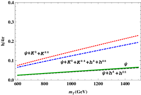
(a)

      

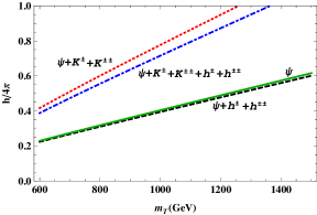
(b)

Figure 6: Contours of the production cross-section $\sigma(pp\to\xi_{\chi}\to\gamma\gamma)$ in femtobarns for the best fit value of 6 fb for (a) mass lower bounds values reported by LHC and (b) $\Gamma=45$ GeV and same mass lower bounds. Here $\beta=\sqrt{3}$ for model A with $\psi=(T^{m},\,J,\,E^{--})$. The green (thick), black (dashed), blue (dot-dashed) and red (dotted) lines correspond to the contributions coming from $\psi$, $\psi+h^{\pm\pm}$, $\psi+K^{\pm}+K^{\pm\pm}+h^{\pm}+h^{\pm\pm}$ and $\psi+K^{\pm}+K^{\pm\pm}$ respectively.

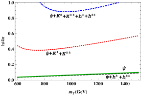
(a)

      

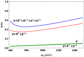
(b)

Figure 7: Contours of the production cross-section $\sigma(pp\to\xi_{\chi}\to\gamma\gamma)$ in femtobarns for the best fit value of 6 fb for (a) mass lower bounds values reported by LHC and (b) asymptotic mass values coming from the form factors $F_{i}$ with $i=0,\,1/2,\,1$. Here $\beta=-\sqrt{3}$ for model A with $\psi=(T,\,J^{m},\,E^{+})$. The green (thick), black (dashed), blue (dot-dashed) and red (dotted) lines correspond to the contributions coming from $\psi$, $\psi+h^{\pm\pm}$, $\psi+K^{\pm}+K^{\pm\pm}+h^{\pm}+h^{\pm\pm}$ and $\psi+K^{\pm}+K^{\pm\pm}$ respectively.

References

• (1) Talk by Jim Olsen, CMS Collaboration, “CMS 13 TeV Results", CERN Jamboree, December 15, 2015. Plots are presented in, http://cms-results.web.cern.ch/cms-results/public-results/preliminary-results/LHC-Jamboree-2015/index.html.
• (2) Talk by Marumi Kado, ATLAS Collaboration, “ATLAS 13 TeV Results", CERN Jamboree, December 15, 2015. Plots are presented in, https://twiki.cern.ch/twiki/bin/view/ AtlasPublic/December2015-13TeV.
• (3) Roberto Franceschini, Gian F. Giudice, Jernej F. Kamenik , Matthew McCullough, Alex Pomarol, Riccardo Rattazzi, Michele Redi, Francesco Riva, Alessandro Strumia, Riccardo Torre, JHEP 1603 (2016) 144; Adam Falkowski, Oren Slone, Tomer Volansky, JHEP 1602 (2016) 152; Keisuke Harigaya, Yasunori Nomura Phys.Lett. B754 (2016) 151-156; Simon Knapen, Tom Melia, Michele Papucci, Kathryn Zurek, Phys.Rev. D93 (2016) no.7, 075020; Dario Buttazzo, Admir Greljo, David Marzocca, Eur.Phys.J. C76 (2016) no.3, 116; Stefano Di Chiara, Luca Marzola, Martti Raidal, Phys.Rev. D93 (2016) no.9, 095018; P. S. Bhupal Dev, Rabindra N. Mohapatra, Yongchao Zhang, JHEP02, 186 (2016); R. Martinez, F. Ochoa and C. F. Sierra, arXiv:1512.05617; Florian Staub, Peter Athron, Lorenzo Basso, Mark D. Goodsell, Dylan Harries, Manuel E. Krauss, Kilian Nickel, Toby Opferkuch, Lorenzo Ubaldi, Avelino Vicente, Alexander Voigt, Precision tools and models to narrow in on the 750 GeV diphoton resonance, arXiv:1602.05581v2 [hep-ph]; S. F. Mantilla, R. Martinez, F. Ochoa, C. F. Sierra, arXiv:1602.05216v2 [hep-ph]; Alessandro Strumia, Interpreting the 750 GeV digamma excess: a review, arXiv:1605.09401 [hep-ph]; Archil Kobakhidze, Fei Wang, Lei Wu, Jin Min Yang, Mengchao Zhang, 750 GeV diphoton resonance in a top and bottom seesaw model, arXiv:1512.05585v4 [hep-ph]; Jorge de Blas, Jose Santiago, Roberto Vega-Morales, New vector bosons and the diphoton excess, arXiv:1512.07229v1 [hep-ph]; D. M. Ghilencea, Hyun Min Lee, Diphoton resonance at 750 GeV in supersymmetry, arXiv:1606.04131 [hep-ph].
• (4) John Ellis, Sebastian A. R. Ellis, J. Quevillon, Veronica Sanz, Tevong You, JHEP 1603 (2016) 176.
• (5) H. Georgi and A. Pais, Phys.Rev. D19, 2746 (1979).
• (6) Pisano, F. and V. Pleitez, Phys. Rev. D46, 410 (1992); R. Foot, O.F. Hernandez, F. Pisano and V. Pleitez, Phys. Rev. D47, 4158 (1993); Nguyen Tuan Anh, Nguyen Anh Ky, Hoang Ngoc Long, Int. J. Mod. Phys. A16, 541 (2001).
• (7) P.H. Frampton, Phys. Rev. Lett. 69, 2889 (1992); D. Ng, Phys. Rev. D49, 4805 (1994).
• (8) Foot, R., H.N. Long and T.A. Tran, Phys. Rev. D50, R34 (1994); H.N. Long, Phys. Rev. D53, 437 (1996); ibid, D54, 4691 (1996); H.N. Long, Mod. Phys. Lett. A13, 1865 (1998)..
• (9) Montero, J.C., F. Pisano and V. Pleitez, Phys. Rev. D47, 2918 (1993); Long. H.N. and T.A. Tran, Mod. Phys. Lett. A9, 2507 (1994); Pisano, F. and V. Pleitez, Phys. Rev. D15, 3865 (1995); Cotaescu, I., Int. J. Mos. Phys. A12, 1483 (1997); Andrzej J. Buras, Fulvia De Fazio, Jennifer Girrbach, Maria V. Carlucci, JHEP 1302 (2013) 023; Andrzej J. Buras, Fulvia De Fazio, Jennifer Girrbach-Noe, JHEP 1408 (2014) 039; Andrzej J. Buras, Fulvia De Fazio, JHEP 1603 (2016) 010.
• (10) Qing-Hong Cao, Yandong Liu, Ke-Pan Xie, Bin Yan, Dong-Ming Zhang, Phys. Rev. D93, 075030 (2016); Sofiane M. Boucenna, Stefano Morisi, Avelino Vicente, Phys.Rev. D93 (2016) no.11, 115008; A. E. Cárcamo Hernández, Ivan Nisandzic, LHC diphoton 750 GeV resonance as an indication of $SU(3)_{C}\times SU(3)_{L}\times U(1)_{X}$ gauge symmetry, arXiv:1512.07165v2 [hep-ph].
• (11) J.S. Bell, R. Jackiw, Nuovo Cim. A60, 47 (1969); S.L. Adler, Phys. Rev. 177, 2426 (1969); D.J. Gross, R. Jackiw, Phys.Rev. D6, 477 (1972). H. Georgi and S. L. Glashow, Phys. Rev. D6, 429 (1972); S. Okubo, Phys. Rev. D16, 3528 (1977); J. Banks and H. Georgi, Phys. Rev. 14, 1159 (1976).
• (12) C. A. de S. Pires, O. P. Ravinez, Phys. Rev. D58, 35008 (1998); C. A. de S. Pires, Phys. Rev. D60, 075013 (1999).
• (13) R. A. Diaz, R. Martinez, J. Mira, J. Alexis Rodriguez, Phys.Lett. B552, 287-292, (2003); R. A. Diaz, R. Martinez, D. Gallego, [arXiv: hep-ph/0505096].
• (14) A. E. Carcamo Hernandez, R. Martinez and F. Ochoa, Phys. Rev. D73, 035007 (2006).
• (15) A. G. Dias, C. A. de S.Pires and P. S. Rodrigues da Silva, Phys. Lett. B628, 85 (2005); A. G. Dias, A. Doff, C. A. de S.Pires and P. S. Rodrigues da Silva, Phys. Rev. D72, 035006 (2005); A. G. Dias, C. A. de S.Pires, P. S. Rodrigues da Silva and A. Sampieri, Phys. Rev. D86, 035007 (2012).
• (16) P. V. Dong, H. N. Long, D. V. Soa and V. V. Vien, Eur. Phys. J. C71, 1544 (2011); P. V. Dong, H. N. Long, C. H. Nam and V. V. Vien, Phys. Rev. D85, 053001 (2012); P. V. Dong, D. T. Huong, M. C. Rodriguez and H. N. Long, J. Mod. Phys. 2, 792 (2011).
• (17) A. E. Cárcamo Hernández, R. Martinez and F. Ochoa, arXiv:1309.6567 [hep-ph]; A. E. Carcamo Hernandez, R. Martinez and F. Ochoa, Phys. Rev. D87, no. 7, 075009 (2013); A. E. C. Hernández, E. C. Mur and R. Martinez, Phys. Rev. D90, no. 7, 073001 (2014); A. E. C. Hernández, R. Martinez and J. Nisperuza, Eur. Phys. J. C75, no. 2, 72 (2015); A. E. Cárcamo Hernández and R. Martinez, Nucl. Phys. B905, 337 (2016); A. E. C. Hernández and R. Martinez, J. Phys. G43, no. 4, 045003 (2016).
• (18) V. V. Vien and H. N. Long, JHEP 1404, 133 (2014); V. V. Vien and H. N. Long, Int. J. Mod. Phys. A30, no. 21, 1550117 (2015); V. V. Vien, A. E. C. Hernández and H. N. Long, arXiv:1601.03300 [hep-ph]; A. E. C. Hernández, H. N. Long and V. V. Vien, Eur. Phys. J. C76, no. 5, 242 (2016).
• (19) S. M. Boucenna, S. Morisi and J. W. F. Valle, Phys. Rev. D90, no. 1, 013005 (2014); S. M. Boucenna, J. W. F. Valle and A. Vicente, Phys. Rev. D92, no. 5, 053001 (2015); S. M. Boucenna, R. M. Fonseca, F. Gonzalez-Canales and J. W. F. Valle, Phys. Rev. D91, no. 3, 031702 (2015).
• (20) J. K. Mizukoshi, C. A. de S.Pires, F. S. Queiroz and P. S. Rodrigues da Silva, Phys. Rev. D 83, 065024 (2011).
• (21) A. G. Dias, C. A. de S.Pires and P. S. Rodrigues da Silva, Phys. Rev. D 82, 035013 (2010).
• (22) J. D. Ruiz-Alvarez, C. A. de S.Pires, F. S. Queiroz, D. Restrepo and P. S. Rodrigues da Silva, Phys. Rev. D 86, 075011 (2012).
• (23) D. Cogollo, A. X. Gonzalez-Morales, F. S. Queiroz and P. R. Teles, JCAP 1411, no. 11, 002 (2014).
• (24) Chris Kelso, H.N. Long, R. Martinez, Farinaldo S. Queiroz, Phys. Rev. D90, 113011 (2014).
• (25) S. L. Glashow, Nucl. Phys. 22, 579 (1961); S. Weinberg, Phys. Rev. Lett. 19, 1264 (1967); A. Salam, in Elementary Particle Theory: Relativistic Groups and Analyticity (Nobel Symposium No. 8), edited by N. Svartholm (Almqvist and Wiksell, Stockholm, 1968), p. 367.
• (26) A. Yu Ignatieu, R. R. Volkas, Phys. Rev. D68, 023518 (2003).
• (27) R. N. Mohapatra, V. Teplitz, Astrophys. J. 478, 29 (1997).
• (28) R. Volkas, Y. Wong, Astropart. Phys. 13, 21 (2000).
• (29) P. B. Pal, Phys.Rev. D52, 1659 (1995).
• (30) A. G. Dias, V. Pleitez and M. D. Tonasse, Phys.Rev. D67, 095008 (2003); A.G. Dias, C. A. de S. Pires and P. S. R. da Silva, Phys.Rev. D68, 115009 (2003); A. G. Dias and V. Pleitez, Phys.Rev. D69, 077702 (2004).
• (31) L.A. Sánchez, W.A. Ponce, and R. Martinez, Phys. Rev. D64, 075013 (2001); W.A. Ponce, J.B. Flórez and L.A. Sánchez, Int. J. Mod. Phys. A17, 643 (2002); W.A. Ponce, Y. Giraldo, and L.A. Sánchez, Phys. Rev.D67, 075001 (2003).
• (32) R. A Diaz, R. Martinez and F. Ochoa, Phys. Rev. D 69, 095009 (2004); Fredy Ochoa, R. Martinez, Phys. Rev D72, 035010 (2005); F. Ochoa, Construcción y estudio fenomenológico de los modelos $SU(3)_{C}\otimes SU(3)_{L}\otimes U(1)_{X}$, Ph.D. Thesis, Universidad Nacional de Colombia (2007).
• (33) P.V. Dong, H.N. Long , H.T. Hung, Phys.Rev. D86, 033002 (2012).
• (34) Doff, A. and F. Pisano, Mod.Phys.Lett. A15 1471-1480 (2000).
• (35) J.F. Gunion, H.E. Haber, G. Kane and S. Dawson. The Higgs Hunter’s Guide. Addison-Wesley Publishing Company. 1990; R. Martinez, M. A. Perez, and J. J. Toscano, Phys. Rev. D 40, 1722 (1989); R. Martinez, M.A. Perez, J.J. Toscano, Phys.Lett. B234 (1990) 503; R. Martinez, M.A. Perez, Nucl.Phys. B347 (1990) 105-119.
• (36) M. Spira, A. Djouadi, D. Graudenz and P. M. Zerwas, Higgs boson production at the LHC, Nucl. Phys. B 453 (1995) 17 [hep-ph/9504378]. A.D. Martin, W.J. Stirling, R.S. Thorne, G. Watt, “Parton distributions for the LHC”, Eur. Phys. J. C63 (2009) 189 [arXiv:0901.0002].
• (37) ATLAS Collaboration, JHEP 12, 55 (2015) ; CMS Collaboration, “Search for leptonic decays of W’ bosons in pp collisions at $\sqrt{s}$ = 8 TeV”, report CMS-PAS-EXO-12-060, March 2013.
• (38) ATLAS Collaboration, Phys. Rev. D 92, 032001 (2015).
• (39) CMS Collaboration, Phys. Rev. D 93, 012003 (2016); ATLAS Collaboration, arXiv:1602.05606 [hep-ex]; CMS Collaboration arXiv:1507.07129 [hep-ex].
• (40) ATLAS Collaboration, JHEP 03, 127 (2016); CMS Collaboration, JHEP 12, 178 (2015); CMS Collaboration, arXiv:1508.07774 [hep-ex].