Complexity of sparse polynomial solving: homotopy on toric varieties and the condition metric

Abstract.

This paper investigates the cost of solving systems of sparse polynomial equations by homotopy continuation. First, a space of systems of $n$-variate polynomial equations is specified through $n$ monomial bases. The natural locus for the roots of those systems is known to be a certain toric variety. This variety is a compactification of $(\mathbb{C}\setminus\{0\})^{n}$, dependent on the monomial bases. A toric Newton operator is defined on that toric variety. Smale’s alpha theory is generalized to provide criteria of quadratic convergence. Two condition numbers are defined and a higher derivative estimate is obtained in this setting. The Newton operator and related condition numbers turn out to be invariant through a group action related to the momentum map. A homotopy algorithm is given, and is proved to terminate after a number of Newton steps which is linear on the condition length of the lifted homotopy path. This generalizes a result from Bezout6.

1. Introduction

The solution of Smale’s 17th problem by Beltrán and Pardo Beltran-Pardo-2009,Beltran-Pardo-2011 and Lairez was a tremendous breakthrough in the theory of solving polynomial systems. Roughly, the cost of finding an approximate solution for a random system of $n$ polynomial equations on $n$ variables is bounded by a polynomial in the input size.

Yet, several unanswered questions may prevent the immediate application of those results and supporting algorithms. One of the main obstructions comes from the way the input size was defined by  Smale-next-century. First the total degree $d_{i}$ of each equation $f_{i}$ is prescribed. Then,

A probability measure must be put on the space of all such $\mathbf{f}$, for each $\mathbf{d}=(d_{1},\dots,d_{n})$ and the time of an algorithm is averaged over the space of $\mathbf{f}$. Is there such an algorithm where the average time is bounded by a polynomial in the number of coefficients of $\mathbf{f}$ (the input size)?

Usually, the probability measure is assumed to be the normal distribution with $0$ average and identity covariance with respect to Weyl’s $U(n+1)$-invariant inner product. The input size of such a system is therefore $\sum_{i=1}^{n}\left(\begin{matrix}d_{i}+n\\ d_{i}\end{matrix}\right)$.

Instead, a lot of the current numerical interest concentrates on systems of equations of the form

(1) $$\begin{array}[]{lcl}F_{1}(\mathbf{Z})&=&\sum_{\mathbf{a}\in A_{1}}f_{i,\mathbf{a}}Z_{1}^{a_{1}}Z_{2}^{a_{2}}\cdots Z_{n}^{a_{n}}\\ &\vdots&\\ F_{n}(\mathbf{Z})&=&\sum_{\mathbf{a}\in A_{n}}f_{i,\mathbf{a}}Z_{1}^{a_{1}}Z_{2}^{a_{2}}\cdots Z_{n}^{a_{n}},\end{array}$$

where each $A_{i}$ is a finite set. The natural input size for those systems is $\sum_{i}\#A_{i}$ which can be exponentially smaller than $\sum_{i=1}^{n}\left(\begin{matrix}d_{i}+n\\ d_{i}\end{matrix}\right)$.

One of the main reasons to find roots of a random system is to use them as a starting point for a homotopy algorithm. Sometimes, only the ‘finite’ roots of a sparse system are needed. Those are the roots in $(\mathbb{C}\setminus\{0\})^{n}$. A famous theorem by Bernstein, Kushnirenko and KhovanskiiBKK bounds the number of such roots in terms of the mixed volume of the convex hulls of the $A_{i}$. This bound is tighter than Bézout’s Theorem. The bound is exact once the roots are taken in the proper compactification of $(\mathbb{C}\setminus\{0\})^{n}$ and counted with multiplicity. This compactification is a particular toric variety. Properly detecting and finding ‘infinite’ roots in this toric variety is also an interesting problem. Finding just one root of a random dense system could be very expensive and would not necessarily provide a finite root of the sparse target system, or even a legitimate ‘infinite’ root in the toric variety. Those considerations lead to the following theoretical questions:

Problem A.

Can a finite zero of a random sparse polynomial system as in equation (1) be found approximately, on the average, in time polynomial in $\sum_{i}\#A_{i}$ with a uniform algorithm?

Problem B.

Can every finite zero of a random polynomial system as in equation (1) be found approximately, on the average, in time polynomial in $\sum_{i}\#A_{i}$ with a uniform algorithm running in parallel, one parallel process for every expected zero?

To simplify Problem B, one can assume that some preliminary information such as a lower mixed subdivision is given as input to the algorithm. An algorithm to find this mixed subdivision in time bounded in terms of mixed volumes and other quermassintegrals was given by Malajovich-Mixed. Implementation issues were also discussed. Jensen provides an alternative symbolic method which can also be used to recover this mixed subdivision.

As a first step towards an investigation of problems  A and B, this paper attempts to develop a theory of homotopy algorithms for sparse polynomial systems by following a parallel with the theory for dense polynomial systems. A key result in the theory was obtained by Bezout6: the cost of homotopy is bounded above by the condition length of the homotopy path (see Section 2). The aim of this paper is to obtain a similar theorem for sparse polynomial systems.

One of the cornerstones of that theory is the concept of $U(n+1)$ invariance [Bezout1, Bezout2, Bezout3, Bezout5, Bezout4, BCSS, Bezout6, Bezout7, Beltran-Pardo-2009, Beltran-Pardo-2011, Burgisser-Cucker, Adaptive]. Unfortunately, unitary action does not preserve the structure of equation  (1). In this paper, the $U(n+1)$ invariance will be replaced by another group action explained in Section 3.

It is convenient to identify sparse polynomials to exponential sums. More formally, let $\mathscr{F}_{A_{i}}$ be the set of expressions of the form $f_{i}(\mathbf{z})=\sum_{\mathbf{a}\in A_{i}}f_{i\mathbf{a}}e^{\mathbf{a}\mathbf{z}}$ and let $\mathbf{f}\in\mathscr{F}_{A_{1}}\times\cdots\times\mathscr{F}_{A_{n}}$ . If $\mathbf{f}(\mathbf{z})=0$ and $e^{\mathbf{z}}=\mathbf{Z}\in(\mathbb{C}\setminus\{0\})^{n}$ then $\mathbf{Z}$ is a finite zero of equation (1). In section 3 we will construct the toric variety $\mathscr{V}$ as the Zariski closure of a non-unique embedding of $(\mathbb{C}\setminus\{0\})^{n}$ into $\mathbb{P}(\mathscr{F}_{A_{1}}^{*})\times\cdots\times\mathbb{P}(\mathscr{F}_{A_{n}}^{*})$. Actual computations require the use of some local chart. We will use a system of ‘logarithmic coordinates’ $[V]:\mathscr{M}\rightarrow\mathscr{V}$ where $\mathscr{M}$ is the quotient of the $z$-space $\mathbb{C}^{n}$ that makes the embedding injective. To every point $x\in\mathscr{M}$ we will associate the local norm $\|\cdot\|_{\mathbf{x}}$ induced by the pull-back of Fubini-Study metric from $\mathscr{V}$. Another possibility discussed in section 6 is to endow $\mathscr{M}$ with a Finsler structure. We will also define a Newton operator on $\mathscr{V}$ which will actually operate on $\mathscr{M}$ as a (locally) linear space. This will avoid all the technicalities associated to Newton iteration on manifolds such as estimating covariant derivatives or approximating geodesics, as required in previous work from Dedieu-Priouret-Malajovich. However $\mathscr{M}$ is still a manifold, with a metric structure associated to each point. We may estimate the distance between two points $\mathbf{x}$, $\mathbf{z}$ through the norm $\|\mathbf{x}-\mathbf{z}\|_{\mathbf{x}}$ on the tangent space $T_{\mathbf{x}}\mathscr{M}$. The subtraction operator above is provided by the linear structure of $\mathbb{C}^{n}$, and it is assumed that representatives $\mathbf{x}$ and $\mathbf{z}$ in $\mathbb{C}^{n}$ minimize the norm.

In this paper, the solution variety is

$$\mathscr{S}_{0}=\left\{\rule{0.0pt}{12.91663pt}(\mathbf{f},\mathbf{x})\in\mathbb{P}(\mathscr{F}_{A_{1}})\times\cdots\times\mathbb{P}(\mathscr{F}_{A_{n}})\times\mathscr{M}:\mathbf{f}(\mathbf{x})=0\right\}$$

We will define two condition numbers $\mu:\mathbb{P}(\mathscr{F}_{A_{1}})\times\cdots\times\mathbb{P}(\mathscr{F}_{A_{n}})\times\mathscr{M}\rightarrow[1,\infty]$ and $\nu:\mathscr{M}\rightarrow[1,\infty]$. Let $\Sigma^{\prime}$ be the set of ill-posed pairs, that is the set of all $(\mathbf{f},\mathbf{x})$ with $\mu(\mathbf{f},\mathbf{x})\nu(\mathbf{x})=\infty$. The condition numbers induce a length structure on $\mathscr{S}_{0}\setminus\Sigma^{\prime}$: the condition length of a rectifiable path $(\mathbf{f}_{t},\mathbf{z}_{t})_{t\in[t_{0},t_{1}]}$ is defined by

$$\mathscr{L}\left(\rule{0.0pt}{10.76385pt}(\mathbf{f}_{t},\mathbf{z}_{t});t_{0},t_{1}\right)=\int_{t_{0}}^{t_{1}}\mu(\mathbf{f}_{t},\mathbf{z}_{t})\nu(\mathbf{z}_{t})\sqrt{\|\dot{\mathbf{f}}_{t}\|_{\mathbf{f}_{t}}^{2}+\|\dot{\mathbf{z}}_{t}\|_{\mathbf{z}_{t}}^{2}}\ \,\mathrm{d}t.$$

This gives $\mathscr{S}_{0}\setminus\Sigma^{\prime}$ the structure of a path-metric space.

Main Theorem A.

Let $(\mathbf{f}_{t},\mathbf{z}_{t})_{t\in[0,T]}$ be a rectifiable path in $\mathscr{S}_{0}\setminus\Sigma^{\prime}$. Let $\mathbf{x}_{0}$ be an approximation for $\mathbf{z}_{0}$, satisfying

$$\frac{1}{2}\mu(\mathbf{f}_{0},\mathbf{z}_{0})\nu(\mathbf{z}_{0})\|\mathbf{z}_{0}-\mathbf{x}_{0}\|_{\mathbf{z}_{0}}\leq u_{0}$$

for the constant $u_{0}=\frac{3-\sqrt{7}}{2}\simeq 0.090994\cdots$. Then, there is a time mesh $0=t_{0}<t_{1}<\cdots<t_{N}=T$ with

$$N\leq\left\lceil 38\ \mathscr{L}\left(\rule{0.0pt}{10.76385pt}(\mathbf{f}_{t},\mathbf{z}_{t});0,T\right)\right\rceil$$

so that the approximation

$$\mathbf{x}_{i+1}={\mathbf{N}}(\mathbf{f}_{t_{i}},\mathbf{x}_{i})$$

produces $\mathbf{y}_{0}=\mathbf{x}_{N}$ with

$$\frac{1}{2}\mu(\mathbf{f}_{T},\mathbf{z}_{T})\nu(\mathbf{z}_{T})\|\mathbf{z}_{T}-\mathbf{y}_{0}\|_{\mathbf{z}_{T}}\leq u_{0}$$

for the same constant $u_{0}$. Moreover, the sequence $\mathbf{y}_{i+1}={\mathbf{N}}(\mathbf{f}_{T},\mathbf{y}_{i})$ is well-defined and satisfies

$$\|\mathbf{y}_{i}-\mathbf{z}_{T}\|_{\mathbf{z}_{T}}\leq 2^{-2^{i}+1}\|\mathbf{y}_{0}-\mathbf{z}_{T}\|_{\mathbf{z}_{T}}.$$

Main Theorem A is not effective, in the sense that the time mesh above is just said to exist. One can get an adaptive criterion for the step size at the price of increasing the complexity bound.

Main Theorem B.

There are constants

$$\alpha_{1}\simeq 0.081239483\cdots\hskip 20.00003pt\text{and}\hskip 20.00003ptu_{1}\simeq 0.039745185\cdots$$

with the following properties: Let $(\mathbf{f}_{t},\mathbf{z}_{t})_{t\in[0,T]}$ be a rectifiable path in $\mathscr{S}_{0}\setminus\Sigma^{\prime}$. Let $\mathbf{x}_{0}$ be an approximation for $\mathbf{z}_{0}$, satisfying

$$\frac{1}{2}\mu(\mathbf{f}_{0},\mathbf{z}_{0})\nu(\mathbf{z}_{0})\|\mathbf{z}_{0}-\mathbf{x}_{0}\|_{\mathbf{z}_{0}}\leq u_{1}.$$

Then one can define $(\mathbf{x}_{i})$ and $(t_{i})$ recursively by

$$\left\{\begin{array}[]{lcl}\mathbf{x}_{i+1}&=&{\mathbf{N}}(\mathbf{f}_{t_{i}},\mathbf{x}_{i})\\ t_{i+1}&=&\min\left(T,\inf\left\{\rule{0.0pt}{10.76385pt}t>t_{i}:\right.\right.\\ &&\left.\left.\hskip 50.00008pt\rule{0.0pt}{10.76385pt}\frac{1}{2}{\mu}(\mathbf{f}_{t},\mathbf{x}_{i+1})\nu(\mathbf{x}_{i+1})\|{\mathbf{N}}_{\mathbf{f}_{t}}(\mathbf{x}_{i+1})-\mathbf{x}_{i+1}\|_{\mathbf{x}_{i+1}}\geq\alpha_{1}\right\}\right).\end{array}\right.$$

Then, $t_{N}=T$ for some $N\leq\left\lceil{59}\mathscr{L}\left(\rule{0.0pt}{10.76385pt}(\mathbf{f}_{t},\mathbf{z}_{t});0,T\right)\right\rceil$. Moreover, the sequence $\mathbf{y}_{0}=\mathbf{x}_{N}$, $\mathbf{y}_{i+1}={\mathbf{N}}_{\mathbf{f}_{T}}(\mathbf{y}_{i})$ is well-defined and satisfies for $i\geq 1$

$$\|\mathbf{y}_{i}-\mathbf{z}_{T}\|_{\mathbf{z}_{T}}\leq 2^{-2^{i-1}-2}\|\mathbf{y}_{0}-\mathbf{y}_{1}\|.$$

The calculation of $t_{i+1}$ requires a subroutine to find the smallest solution $t>t_{i}$ of the equation

$$\frac{1}{2}{\mu}(\mathbf{f}_{t},\mathbf{x}_{i+1})\nu(\mathbf{x}_{i+1})\|{\mathbf{N}}_{\mathbf{f}_{t}}(\mathbf{x}_{i+1})-\mathbf{x}_{i+1}\|_{\mathbf{x}_{i+1}}=\alpha_{1}.$$

Obvious modifications in the algorithm allow for approximate computations in that subroutine. Similar results were known for the dense setting [Beltran2011, Adaptive, Beltran-Leykin]. The constants in Main Theorem B are not supposed to be sharp.

Last but not least, the methods in this paper may offer a better alternative than projective Newton for approximating certain roots at ‘toric infinity’. We will show this through an example.

Running example, part 1.

The family

(2) $$\mathbf{f}_{t}(X,Y)=\begin{pmatrix}tX-tXY+Y^{2}-t^{2}Y^{3}\\ X+XY-Y^{2}-Y^{3}.\end{pmatrix}$$

admits two ‘finite’ solutions on the toric variety $\mathscr{V}$, namely $(t^{-2},t^{-1})$ and $(-\frac{1+t^{2}}{2t},$ $-1)$. When $t\rightarrow 0$, both solutions converge to different points at toric ‘infinity’ and those can be efficiently approximated. We will show in Section 3 that

$$\mathscr{L}\left(\rule{0.0pt}{10.76385pt}\left(\mathbf{f}_{t},(x_{t},y_{t})\right);\epsilon,1\right)\in\Theta(\log(1/\epsilon))$$

where $(x,y)=(\log(X),\log(Y))$. In comparison, we show in Section 2 that the condition length $L$ for the homogeneous setting as in [Bezout6] satisfies

$$L\left(\rule{0.0pt}{10.76385pt}(\mathbf{f}_{t},[X_{t}:Y_{t}:1]);\epsilon,1\right)\in{\Omega(1/\epsilon)}.$$

This amounts to an exponentially worse bound on the number of homotopy steps, due to the fact that in projective space the two solutions are the undistinguishable on the limit. Indeed, $\lim_{t\rightarrow 0}[X_{t}:Y_{t}:1]=[1:0:0]$ for both curves.

This paper is organized as follows. Section 2 revisits known results about alpha-theory, for reference and conceptual clarification. All the main results and constructs of this paper are contained in Section 3. Among them, the construction of the toric variety, the Newton operator and the momentum map action. Main theorems A and B are proved, but the proofs of intermediate results are postponed. Section 4 contains distortion bounds that allow to switch between charts in $\mathscr{M}$. The remaining technical results are proved in Section 5.

In section 6 an alternative, more natural Finsler structure on the toric variety $\mathscr{V}$ is introduced. All the theorems in this paper are also valid if the Hermitian structure is replaced by this Finsler structure, and some bounds actually become sharper. A short summary and some short remarks close the paper in section 7

Acknowledgements:

The author would like to thank Carlos Beltrán, Bernardo Freitas Paulo da Costa, Felipe Bottega Diniz and two anonymous referees for their suggestions and improvements.

2. Projective Newton iteration revisited

In this section we revisit some classical results about Newton iteration, such as Smale’s quadratic convergence theorems. Then we recall the corresponding results for projective Newton iteration. By understanding projective Newton as an algorithm operating on vector bundles, we highlight some subtle differences between the gamma theorem which extends naturally to projective space, and the alpha theorem.

2.1. Classical theorems

Let $\mathbf{f}:\mathbb{E}\rightarrow\mathbb{F}$ be an analytic mapping between real or complex Banach spaces. Whenever $D\mathbf{f}(\mathbf{x})$ is invertible, Newton iteration is defined by

$$\begin{array}[]{lrcl}{\mathbf{N}}_{\mathbf{f}}:&\mathbb{E}&\longrightarrow&\mathbb{F}\\ &\mathbf{x}&\longmapsto&\mathbf{x}-D\mathbf{f}(\mathbf{x})^{-1}\mathbf{f}(\mathbf{x})\end{array}$$

Smale’s invariants for Newton iterations are:

$$\beta(\mathbf{f},\mathbf{x})=\left\|D\mathbf{f}(\mathbf{x})^{-1}\mathbf{f}(\mathbf{x})\right\|,$$

$$\gamma(\mathbf{f},\mathbf{x})=\max_{k\geq 2}\left(\frac{1}{k!}\left\|D\mathbf{f}(\mathbf{x})^{-1}D^{k}\mathbf{f}(\mathbf{x})\right\|\right)^{\frac{1}{k-1}}$$

and $\alpha(\mathbf{f},\mathbf{x})=\beta(\mathbf{f},\mathbf{x})\gamma(\mathbf{f},\mathbf{x})$. If $D\mathbf{f}(\mathbf{x})$ fails to be surjective at $\mathbf{x}$, then $\alpha(\mathbf{f},\mathbf{x})=\beta(\mathbf{f},\mathbf{x})=\gamma(\mathbf{f},\mathbf{x})=\infty$. Recall also the teminology: a zero $\mathbf{z}$ of $\mathbf{f}$ is said to be degenerate if $D\mathbf{f}(\mathbf{z})$ is not surjective, otherwise it is non-degenerate. The domain of $\mathbf{f}$ will be denoted $\mathcal{D}_{\mathbf{f}}$ and $B(\mathbf{x},r)$ will be the radius $r$ ball around $\mathbf{x}$. The following two results are due to Smale-PE. The constant $\alpha_{0}$ below is due to Wang-Xing-Hua. Proofs can be found on textbooks or lecture notes such as [BCSS, Malajovich-nonlinear, Malajovich-UIMP].

Theorem 2.1.1 ($\gamma$-theorem).

Let $\boldsymbol{\zeta}\in\mathbb{E}$ be a non-degenerate zero of $f$. If $x_{0}\in\mathbb{E}$ satisfies

$$\|\boldsymbol{\zeta}-\mathbf{x}_{0}\|\gamma(\mathbf{f},\boldsymbol{\zeta})\leq\frac{3-\sqrt{7}}{2}$$

and $B(\boldsymbol{\zeta},\|\boldsymbol{\zeta}-\mathbf{x}_{0}\|)\subseteq\mathcal{D}_{\mathbf{f}}$, then the sequence $\mathbf{x}_{i+1}={\mathbf{N}}_{\mathbf{f}}(\mathbf{x}_{i})$ is well-defined and

$$\|\boldsymbol{\zeta}-\mathbf{x}_{i}\|\leq 2^{-2^{i}+1}\|\boldsymbol{\zeta}-\mathbf{x}_{0}\|.$$

Theorem 2.1.2 ($\alpha$-theorem).

Let

$$\alpha\leq\alpha_{0}=\frac{13-3\sqrt{17}}{4},$$

$$r_{0}=\frac{1+\alpha-\sqrt{1-6\alpha+\alpha^{2}}}{4\alpha}\text{ and }r_{1}=\frac{1-3\alpha-\sqrt{1-6\alpha+\alpha^{2}}}{4\alpha}.$$

If $\mathbf{x}_{0}\in\mathbb{E}$ satisfies $\alpha(\mathbf{f},\mathbf{x}_{0})\leq\alpha$, and $B({\mathbf{x}_{0}},r_{0}\beta(\mathbf{f},\mathbf{x}_{0}))\subseteq\mathcal{D}_{\mathbf{f}}$, then the sequence defined recursively by $\mathbf{x}_{i+1}={\mathbf{N}}_{\mathbf{f}}(\mathbf{x}_{i})$ is well-defined and converges to a limit $\boldsymbol{\zeta}$ so that ${\mathbf{f}}(\boldsymbol{\zeta})=0$. Furthermore,

1. $\|\mathbf{x}_{i}-\boldsymbol{\zeta}\|\leq 2^{-2^{i}+1}\|\mathbf{x}_{1}-\mathbf{x}_{0}\|$

2. $\|\mathbf{x}_{0}-\boldsymbol{\zeta}\|\leq r_{0}\beta(\mathbf{f},\mathbf{x}_{0})$

3. $\|\mathbf{x}_{1}-\boldsymbol{\zeta}\|\leq r_{1}\beta(\mathbf{f},\mathbf{x}_{0}).$

2.2. The case for projective Newton

Polynomial equations in $\mathbb{C}^{n}$ are poorly conditionned when a root ‘approaches’ infinity. For instance, the affine system of equations

$$\left\{\begin{array}[]{ccc}\epsilon x-1&=&0\\ y-1&=&0\end{array}\right.$$

has solution $(\epsilon^{-1},1)$. A small perturbation of the first coefficient by (say) $\delta$ may change the solution to $((\epsilon-\delta)^{-1},1)$. The absolute condition number is by definition $\left|\frac{\partial}{\partial\delta}_{|\delta=0}\ \frac{1}{\epsilon-\delta}\right|=\epsilon^{-2}$, while the relative condition number is the absolute condition number divided by the limit value $\epsilon^{-1}$, namely $\epsilon^{-1}$.

This source of ill-posedness was noticed by Bezout1*section I-4. In comparison, the theory was greatly simplified by homogenizing equations and then performing Newton iteration on projective space. On the previous example, the homogenized system is

$$\left\{\begin{array}[]{ccc}\epsilon x-z&=&0\\ y-z&=&0\end{array}\right.$$

and the solution $\left[\epsilon^{-1}:1:1\right]=\left[1:\epsilon:\epsilon\right]$ has a well-defined limit as $\epsilon\rightarrow{0}$.

Those ideas require the introduction of an appropiate Newton operator. One possibility is to perform Newton iteration in $\mathbb{C}^{n+1}$ using the Moore-Penrose pseudo-inverse as AllgowerGeorg, or charts as Morgan. However, the projective Newton operator introduced by ShubProjective allowed for a more natural development of the theory.

2.3. The line bundle $\mathcal{O}(d)$

Homogeneous polynomials do not have a well-defined value on projective space $\mathbb{P}^{n}$. A classical construction in algebraic geometry is to represent homogeneous degree $d$ polynomials as sections of the line bundle $\mathbb{C}\rightarrow\mathcal{O}(d)\stackrel{{\scriptstyle\pi}}{{\rightarrow}}{\mathbb{P}^{n}}$ with total space $\mathcal{O}(d)$ equal to the quotient of $(\mathbb{C}^{n+1}\setminus\{0\})\times\mathbb{C}$ by the $\mathbb{C}_{\times}$ group action

$$\lambda(\mathbf{x},y)=(\lambda\mathbf{x},\lambda^{d}y).$$

When no confusion can arise, we will use the same notation for a fiber bundle and its total space. Through this paper, brackets denote the equivalence class under a prescribed group action. For instance, $\left[\mathbf{x}\right]\in\mathbb{P}^{n}$ will be the equivalence class of $\mathbf{x}\in\mathbb{C}^{n+1}\setminus\{0\}$ with respect to scalings, and $\left[\mathbf{x},y\right]\in\mathcal{O}(d)$ will be the equivalence class of $(\mathbf{x},y)$ under the group action above. Under this notation, the projection operator $\pi:\mathcal{O}(d)\rightarrow\mathbb{P}^{n}$ is just $\left[\mathbf{x},y\right]\mapsto\left[\mathbf{x}\right]$.

To a homogeneous degree $d$ polynomial $f$, one associates the section $s_{f}:\left[\mathbf{x}\right]\mapsto\left[\mathbf{x},f(\mathbf{x})\right]$. The reader should check that this is independent of the choice of the representative $\mathbf{x}$ for $\left[\mathbf{x}\right]$.

2.4. Systems of equations

Let $d_{1},\dots,d_{n}\in\mathbb{N}$ be fixed through this section. We consider the vector bundle $\mathscr{E}=\mathcal{O}(d_{1})\oplus\cdots\oplus\mathcal{O}(d_{n})$. Denoting also by $\mathscr{E}$ its total space, we may write this bundle as $\mathbb{C}^{n}\rightarrow\mathscr{E}\stackrel{{\scriptstyle\pi}}{{\rightarrow}}{\mathbb{P}^{n}}$. The total space $\mathscr{E}$ is the quotient of $(\mathbb{C}^{n+1}\setminus\{0\})\times\mathbb{C}^{n}$ by the $\mathbb{C}_{\times}$ group action

$$\lambda(\mathbf{x},y_{1},\dots,y_{n})=(\lambda\mathbf{x},\lambda^{d_{1}}y_{1},\dots,\lambda^{d_{n}}y_{n}).$$

The projection map takes $[\mathbf{x},\mathbf{y}]$ into $[\mathbf{x}]$.

To a system $(f_{1},\dots,f_{n})$ of homogeneous polynomials of degree $(d_{1},\dots,d_{n})$, one associates the section of the vector bundle

$$\begin{array}[]{lrcl}s_{(f_{1},\dots,f_{n})}:&\mathbb{P}^{n}&\longrightarrow&\mathscr{E}\\ &\left[\mathbf{x}\right]&\longmapsto&\left[\mathbf{x},f_{1}(\mathbf{x}),\dots,f_{n}(\mathbf{x})\right]\end{array}.$$

The brackets on the right denote quotient with respect to the multiplicative group action $\lambda(\mathbf{x},y_{1},\dots,y_{n})=(\lambda\mathbf{x},\lambda^{d_{1}}y_{1},\dots,\lambda^{d_{n}}y_{n})$. The tangent space of $\mathbb{P}^{n}$ at $\mathbf{x}$ is the linear space $\mathbf{x}^{\perp}\subset\mathbb{C}^{n+1}$ with the inner product $\|\mathbf{x}\|^{-2}\langle\cdot,\cdot\rangle$. We can define a local map from $T_{\left[\mathbf{x}\right]}\mathbb{P}^{n}$ into the fiber above $\left[\mathbf{x}\right]$, namely

$$\begin{array}[]{lrcl}S_{\mathbf{f},\mathbf{x}}:&T_{\left[\mathbf{x}\right]}\mathbb{P}^{n}={\mathbf{x}^{\perp}}&\longrightarrow&\pi^{-1}(\left[\mathbf{x}\right])\cong\mathbb{C}^{n}\\ &\dot{\mathbf{x}}&\longmapsto&f_{1}(\mathbf{x}+\dot{\mathbf{x}}),\dots,f_{n}(\mathbf{x}+\dot{\mathbf{x}})\end{array}$$

Since this $S_{\mathbf{f},\mathbf{x}}$ is a function between linear spaces, we can define the local Newton operator associated to $s_{\mathbf{f}}$ as the Newton operator for $S_{\mathbf{f},\mathbf{x}}$:

$$\begin{array}[]{lrcl}{\mathbf{N}}_{\mathbf{f},\mathbf{x}}:&T_{\left[\mathbf{x}\right]}\mathbb{P}^{n}&\longrightarrow&T_{\left[\mathbf{x}\right]}\mathbb{P}^{n}\\ &\dot{\mathbf{x}}&\longmapsto&\dot{\mathbf{x}}-\left(D\mathbf{f}(\mathbf{x}+\dot{\mathbf{x}})_{|{{\mathbf{x}}^{\perp}}}\right)^{-1}\mathbf{f}(\mathbf{x}+\dot{\mathbf{x}})\end{array}$$

The projective Newton operator is

$$\begin{array}[]{lrcl}{\mathbf{N}}^{\mathrm{proj}}_{\mathbf{f}}:&\mathbb{P}^{n}&\longrightarrow&\mathbb{P}^{n}\\ &\left[\mathbf{x}\right]&\longmapsto&\left[\mathbf{x}+{\mathbf{N}}_{\mathbf{f},\mathbf{x}}(0)\right].\end{array}$$

Remark 2.4.1.

Explicit expressions for the projective Newton operator are

$${\mathbf{N}}^{\mathrm{proj}}_{\mathbf{f}}(\left[\mathbf{x}\right])=\left[\mathbf{x}-D\mathbf{f}(\mathbf{x})_{|\mathbf{x}^{\perp}}^{-1}\mathbf{f}(\mathbf{x})\right]=\left[\mathbf{x}-\begin{pmatrix}D\mathbf{f}(\mathbf{x})\\ \mathbf{x}^{*}\end{pmatrix}^{-1}\begin{pmatrix}\mathbf{f}(\mathbf{x})\\ 0\end{pmatrix}\right].$$

2.5. Alpha theory

Smale’s invariants for the projective Newton operator are

$$\beta(\mathbf{f},\left[\mathbf{x}\right])=\frac{1}{\|\mathbf{x}\|}\left\|D\mathbf{f}(\mathbf{x})_{|\mathbf{x}^{\perp}}^{-1}\mathbf{f}(\mathbf{x})\right\|,$$

$$\gamma(\mathbf{f},\left[\mathbf{x}\right])=\|\mathbf{x}\|\max_{k\geq 2}\left(\frac{1}{k!}\left\|D\mathbf{f}(\mathbf{x})_{|\mathbf{x}^{\perp}}^{-1}D^{k}\mathbf{f}(\mathbf{x})\right\|\right)^{\frac{1}{k-1}}$$

and of course $\alpha(\mathbf{f},\left[\mathbf{x}\right])=\beta(\mathbf{f},\left[\mathbf{x}\right])\gamma(\mathbf{f},\left[\mathbf{x}\right])$.

We will denote by $d(\left[\mathbf{x}\right],\left[\mathbf{y}\right])$ the Riemannian (Fubini-Study) distance in projective space and by $d_{T}(\left[\mathbf{x}\right],\left[\mathbf{y}\right])=\tan d(\left[\mathbf{x}\right],\left[\mathbf{y}\right])$ the ‘tangential distance’. This is not a metric, since the triangle inequality fails. However, if $\dot{\mathbf{x}}\perp\mathbf{x}$, then

$$d_{T}(\left[\mathbf{x}\right],\left[\mathbf{x}+\dot{\mathbf{x}}\right])=\frac{\|\dot{\mathbf{x}}\|}{\|\mathbf{x}\|}$$

is the norm in $T_{\left[\mathbf{x}\right]}\mathbb{P}^{n}$.

Theorem 2.5.1 ($\gamma$-theorem).

Let $\left[\boldsymbol{\zeta}\right]\in\mathbb{P}^{n}$ be a non-degenerate zero of $f$. If $\left[\mathbf{x}_{0}\right]\in\mathbb{P}^{n}$ satisfies

$$d_{T}(\left[\boldsymbol{\zeta}\right],\left[\mathbf{x}_{0}\right])\gamma(\mathbf{f},\left[\boldsymbol{\zeta}\right])\leq\frac{3-\sqrt{7}}{2},$$

then the sequence $\left[\mathbf{x}_{i+1}\right]={\mathbf{N}}^{\mathrm{proj}}_{{\mathbf{f}}}(\left[\mathbf{x}_{i}\right])$ is well-defined and

$$d_{T}(\left[\boldsymbol{\zeta}\right],\left[\mathbf{x}_{i}\right])\leq 2^{-2^{i}+1}d_{T}(\left[\boldsymbol{\zeta}\right],\left[\mathbf{x}_{0}\right]).$$

This first appeared in the book by BCSS*Th.1 p.263. Burgisser-Cucker*Th.16.38 provided a refinement of this theorem, not necessary for this paper. One can also state an alpha-theorem for the projective Newton iteration, but the sharpest $\alpha_{0}$ constant seems to be unknown. Instead we can apply Theorem 2.1.2 to the local Newton operator.

Theorem 2.5.2 (Tangential $\alpha$-theorem).

Let

$$\alpha\leq\alpha_{0}=\frac{13-3\sqrt{17}}{4}.$$

Let

$$r_{0}=\frac{1+\alpha-\sqrt{1-6\alpha+\alpha^{2}}}{4\alpha}\text{ and }r_{1}=\frac{1-3\alpha-\sqrt{1-6\alpha+\alpha^{2}}}{4\alpha}.$$

If $\left[{\mathbf{x}_{0}}\right]\in\mathbb{P}^{n}$ satisfies $\alpha(\mathbf{f},\left[\mathbf{x}_{0}\right])\leq\alpha$, then the sequence defined recursively by $\dot{\mathbf{x}}_{0}=0$, $\dot{\mathbf{x}}_{i+1}={\mathbf{N}}_{\mathbf{f},\mathbf{x}}(\dot{\mathbf{x}}_{i})$ is well-defined and converges to a limit $\dot{\mathbf{x}}^{*}$ so that $\left[\boldsymbol{\zeta}\right]\stackrel{{\scriptstyle\mathrm{def}}}{{=}}\left[{\mathbf{x}_{0}}+\dot{\mathbf{x}}^{*}\right]$ is a zero of $\mathbf{f}$. Furthermore,

1. $\|\dot{\mathbf{x}}_{i}-\dot{\mathbf{x}}^{*}\|\leq 2^{-2^{i}+1}\|\dot{\mathbf{x}}^{*}\|$

2. $d_{T}(\left[{\mathbf{x}_{0}}+\dot{\mathbf{x}}_{i}\right],\left[\boldsymbol{\zeta}\right])\leq 2^{-2^{i}+1}d_{T}(\left[{\mathbf{x}_{0}}\right],\left[\boldsymbol{\zeta}\right])$

3. $d_{T}(\left[\mathbf{x}_{0}\right],\left[\boldsymbol{\zeta}\right])\leq r_{0}\beta(\mathbf{f},\left[\mathbf{x}_{0}\right])$

4. $d_{T}({\mathbf{N}}^{\mathrm{proj}}_{\mathbf{f}}(\left[\mathbf{x}_{0}\right]),\left[\boldsymbol{\zeta}\right])\leq r_{1}\beta(\mathbf{f},\left[\mathbf{x}_{0}\right]).$

We will need to borrow Lemma 2(4) p.264 from BCSS. Since I am not satisfied with the published proof, I included an alternate one in the appendix.

Lemma 2.5.3.

Suppose that $\mathbf{x},\mathbf{y},\boldsymbol{\zeta}\in\mathbb{C}^{n+1}$ with $\boldsymbol{\zeta}-\mathbf{x}\perp\mathbf{x}$, $\mathbf{y}-\mathbf{x}\perp\mathbf{x}$ and $\|\mathbf{y}-\boldsymbol{\zeta}\|\leq\|\mathbf{x}-\boldsymbol{\zeta}\|$. Then,

$$\frac{\|\pi(\mathbf{y})-\boldsymbol{\zeta}\|}{\|\boldsymbol{\zeta}\|}\leq\frac{\|\mathbf{y}-\boldsymbol{\zeta}\|}{\|\mathbf{x}\|}$$

where $\pi(\mathbf{y})=\frac{\|\boldsymbol{\zeta}\|^{2}}{\langle\mathbf{y},\boldsymbol{\zeta}\rangle}\mathbf{y}$ is the radial projection onto the affine plane $\boldsymbol{\zeta}+\boldsymbol{\zeta}^{\perp}$.

Proof of Theorem 2.5.2.

Item (a) is Theorem 2.1.2 in $\mathbf{x}_{0}+\mathbf{x}_{0}^{\perp}\cong\mathbb{C}^{n}$. Item (b) is a particular case of the Lemma 2.5.3 above, namely

$$d_{T}(\left[{\mathbf{x}_{0}}+\dot{\mathbf{x}}_{i}\right],\left[\boldsymbol{\zeta}\right])=\frac{\|\pi(\mathbf{y})-\boldsymbol{\zeta}\|}{\|\boldsymbol{\zeta}\|}\leq\frac{\|\mathbf{y}-\boldsymbol{\zeta}\|}{\|\mathbf{x}\|}=\|\dot{\mathbf{x}}_{i}-\dot{\mathbf{x}}^{*}\|/\|\mathbf{x}_{0}\|$$

for $\mathbf{x}=\mathbf{x}_{0}$, $\mathbf{y}={\mathbf{x}_{0}}+\dot{\mathbf{x}}_{1}$ and $\boldsymbol{\zeta}=\mathbf{x}+\dot{\mathbf{x}}^{*}$. Items (c) and (d) follow from Theorem  2.1.2(b,c) and from estimates

$$d_{T}(\left[\mathbf{x}_{0}\right],\left[\boldsymbol{\zeta})\right])=\|\dot{\mathbf{x}}^{*}\|{/\|\mathbf{x}_{0}\|}\hskip 20.00003pt\text{ and }\hskip 20.00003ptd_{T}(\left[\mathbf{x}_{1}\right],\left[\boldsymbol{\zeta})\right])\leq\|\dot{\mathbf{x}}_{1}-\dot{\mathbf{x}}^{*}\|{/\|\mathbf{x}_{0}\|}$$

the last one as above with $\mathbf{y}=\mathbf{x}+\dot{\mathbf{x}}_{1}=\mathbf{x}_{1}$. ∎

2.6. Homotopy and the condition length

Let $\mathscr{H}_{d}$ be the complex space of degree $d$ homogeneous polynomials on $n+1$ variables, endowed with Weyl’s $U(n+1)$-invariant inner product. Let $\mathscr{H}_{(d_{1},\dots,d_{n})}=\mathscr{H}_{d_{1}}\times\cdots\times\mathscr{H}_{d_{n}}$. The invariant condition number $\mu:\mathbb{P}(\mathscr{H}_{(d_{1},\dots,d_{n})})\times\mathbb{P}^{n}\rightarrow[\sqrt{n},\infty]$ defined by Bezout1 is

(3) $$\mu(\mathbf{f},\mathbf{x})=\|\mathbf{f}\|\left\|D\mathbf{f}(\mathbf{x})_{\mathbf{x}^{\perp}}^{-1}\begin{pmatrix}\|\mathbf{x}\|^{d_{1}-1}\sqrt{d_{1}}\\ &\ddots\\ &&\|\mathbf{x}\|^{d_{n}-1}\sqrt{d_{n}}\end{pmatrix}\right\|$$

with the operator $2$-norm assumed. The minimum of $\mu(\mathbf{f},\mathbf{x})=\sqrt{n}$ is actually attained for $f_{i}(\mathbf{x})=\sqrt{d_{i}}\mathbf{x}_{0}^{d_{i}-1}\mathbf{x}_{i}$ at $\mathbf{x}=\mathrm{e}_{0}$. At this system, $\|f_{i}\|=1$ in Weyl’s metric and therefore $\|\mathbf{f}\|=\sqrt{n}$. The main complexity result that we want to emulate is:

Theorem 2.6.1.

[Bezout6]*Th.3 There is a constant $C_{1}>0$, such that: if $(\mathbf{f}_{t},\mathbf{z}_{t})$, $t_{0}\leq t\leq t_{1}$ is a $\mathcal{C}^{1}$ path in $\mathscr{S}_{0}=\{([\mathbf{f}],[\mathbf{z}]):\mathbf{f}(\mathbf{z})=0\}$, then

$$C_{1}(\max d_{i})^{3/2}\int_{t_{0}}^{t_{1}}\mu(\mathbf{f}_{t},\mathbf{z}_{t})\sqrt{\|\dot{\mathbf{f}}_{t}\|_{\mathbf{f}_{t}}^{2}+\|\dot{\mathbf{z}}_{t}\|_{\mathbf{z}_{t}}^{2}}\ \,\mathrm{d}t$$

steps of the projective Newton method are sufficient to continue an approximate zero $\mathbf{x}_{0}$ of $\mathbf{f}_{t_{0}}$ with associated zero $\mathbf{z}_{0}$ to an approximate zero $\mathbf{x}_{1}$ of $\mathbf{f}_{t_{1}}$ with associated zero $\mathbf{z}_{t_{1}}$.

In the context of dense polynomial systems, the condition length relates algorithmic issues to geometrical properties of the solution variety [Bezout7, Boito-Dedieu, BDMS1, BDMS2]. Adaptive algorithms exploiting the condition length were presented by Beltran-Leykin and Adaptive. Hauenstein-Liddell obtained a similar algorithm for constant term homotopy. This allowed them to replace the condition number by Smale’s $\gamma$ invariant in the definition of condition length. ABBCS used the condition length complexity estimates to derive an average complexity result. Condition metrics can also be studied for their own sake as in [BDMS1, CriadoDelRey].

Running example, part 2.

We estimate now the condition length for the two solution paths in the example of equation (2). Let $\mathbf{Z}_{t}=(X_{t},Y_{t},1)$ so that

$$\mathbf{Z}_{t}^{(1)}=\begin{pmatrix}t^{-2}\\ t^{-1}\\ 1\end{pmatrix}\hskip 10.00002pt\text{and}\hskip 10.00002pt\mathbf{Z}_{t}^{(2)}=\begin{pmatrix}-\frac{t^{2}+1}{2t}\\ -1\\ 1\end{pmatrix}.$$

In norms,

$$\|\mathbf{Z}_{t}^{(1)}\|^{2}=t^{-4}+t^{-2}+1\hskip 10.00002pt\text{and}\hskip 10.00002pt\|\mathbf{Z}_{t}^{(2)}\|^{2}=\frac{1}{4}t^{-2}+\frac{5}{2}+\frac{1}{4}t^{2}$$

The Weyl norm of $\mathbf{f}_{t}$ satisfies $\|\mathbf{f}_{t}\|^{2}=\frac{13}{6}+\frac{1}{2}t^{2}+t^{4}$. Instead of evaluating the norm of $(D\mathbf{f}_{t}(\mathbf{Z}^{(i)}(t))_{(\mathbf{Z}^{(i)}(t))^{\perp}})^{-1}$, we compute

$$D\mathbf{f}_{t}(\mathbf{Z}^{(1)}(t))D\mathbf{f}_{t}(\mathbf{Z}^{(1)}(t))^{*}=\begin{pmatrix}t^{2}-2t+10-6t^{-1}+5t^{-2}&t+5t^{-1}+4t^{-2}+2t^{-4}\\ t+5t^{-1}+4t^{-2}+2t^{-4}&1+2t^{-1}+5t^{-2}+8t^{-3}+5t^{-4}+2t^{-5}+t^{-6}\end{pmatrix}$$

and

$$D\mathbf{f}_{t}(\mathbf{Z}^{(2)}(t))D\mathbf{f}_{t}(\mathbf{Z}^{(2)}(t))^{*}=\begin{pmatrix}\frac{17}{2}t^{4}+13t^{2}+\frac{5}{2}&2t^{3}+4t^{2}+3t+2+t^{-1}\\ 2t^{3}+4t^{2}+3t+2+t^{-1}&\frac{1}{2}t^{2}+2t+3+2t^{-1}+\frac{1}{2}t^{-2}\end{pmatrix}.$$

Since

$$(\mu^{(i)})^{2}=\left(\mu^{(i)}(\mathbf{f}_{t},\mathbf{Z}^{(i)}(t))\right)^{2}=3\|\mathbf{Z}^{(i)}(t)\|^{4}\|\mathbf{f}_{t}\|^{2}\left\|\left(D\mathbf{f}_{t}(\mathbf{Z}^{(i)}(t))D\mathbf{f}_{t}(\mathbf{Z}^{(i)}(t))^{*}\right)^{-1}\right\|,$$

we first expand the inverse of

$$D\mathbf{f}_{t}(\mathbf{Z}^{(i)}(t))D\mathbf{f}_{t}(\mathbf{Z}^{(i)}(t))^{*}$$

into its Laurent series around zero using the Maxima computer algebra system [MAXIMA]. The condition length for paths $(\mathbf{f}_{t},\mathbf{Z}_{t}^{(1)})$ and ,$(\mathbf{f}_{t},\mathbf{Z}_{t}^{(2)})$ is computed in Table 1. Overall, the condition length $L$ satisfies

$$L((\mathbf{f}_{t},\mathbf{Z}_{t}^{(1)}),\epsilon,1)=\int_{\epsilon}^{1}\mu(\mathbf{f}_{t},\mathbf{z}_{t})\sqrt{\|\dot{\mathbf{f}}_{t}\|_{\mathbf{f}_{t}}^{2}+\|\dot{\mathbf{z}}_{t}\|_{\mathbf{z}_{t}}^{2}}\ \,\mathrm{d}t\in\Theta(\epsilon^{-2})$$

as claimed in the introduction. This is also the best known upper bound for the number of projective Newton steps in a homotopy algorithm going from $f_{1}$ to $f_{\epsilon}$.

$i$ $1$ $2$ $d_{1,2}$ $3$ $3$ $\|\mathbf{Z}^{(i)}(t)\|^{4}$ $t^{-8}+O(t^{-6})$ $\frac{1}{16}t^{-4}+O(t^{-3})$ $\|\mathbf{f}_{t}\|^{2}$ $\frac{13}{6}+O(t^{2})$ $\frac{13}{6}+O(t^{2})$ $\|\left(D\mathbf{f}_{t}D\mathbf{f}_{t}^{*}\right)^{-1}\|$ $t^{2}+O(t^{3})$ $2+O(t)$ $(\mu^{(i)})^{2}$ $\frac{13}{2}t^{-6}+O(t^{-5})$ $\frac{13}{16}t^{-4}+O(t^{-3})$ $\left\|\frac{\partial}{\partial t}\mathbf{f}_{t}\right\|_{\mathbf{f}_{t}}^{2}$ $\frac{3}{13}+O(t^{2})$ $\frac{3}{13}+O(t^{2})$ $\left\|\frac{\partial}{\partial t}\mathbf{Z}^{(i)}(t)\right\|_{\mathbf{Z}^{(i)}(t)}^{2}$ $1+O(t^{2})$ $8+O(t^{2})$ $\left(\mu^{(i)}\left\|\frac{\partial}{\partial t}\left(\mathbf{f}_{t},\mathbf{Z}^{(i)}(t)\right)\right\|_{\left(\mathbf{f}_{t},\mathbf{Z}^{(i)}(t)\right)}\right)^{2}$ $8t^{-6}+O(t^{-5})$ $\frac{107}{16}t^{-4}+O(t^{-3})$ $\mu^{(i)}\left\|\frac{\partial}{\partial t}\left(\mathbf{f}_{t},\mathbf{Z}^{(i)}(t)\right)\right\|_{\left(\mathbf{f}_{t},\mathbf{Z}^{(i)}(t)\right)}$ $\sqrt{8}t^{-3}+O(t^{-2})$ $\sqrt{\frac{107}{16}}t^{-2}+O(t^{-1})$ $L((\mathbf{f}_{t},\mathbf{Z}_{t}^{(i)});\epsilon,1)=\int_{\epsilon}^{1}\mu^{(i)}\|\cdots\|\,\mathrm{d}t$ $\sqrt{2}\epsilon^{-2}+O(\epsilon^{-1})$ $\sqrt{\frac{107}{16}}\epsilon^{-1}+O(\log(\epsilon^{-1}))$

Table 1. Computation of the condition length in the homogeneous setting.

3. Toric Newton iteration, condition and homotopy

The two solution paths for equation (2) from the running example converge to the same point in projective space. Indeed, the solution paths $(t^{-2},t^{-1})$ and $(-\frac{1+t^{2}}{2t},-1)$ correspond to solution paths $[1:t:t^{2}]$ and $[1+2t^{2}:2t:-2t]$ in $\mathbb{P}^{2}$. When $t=0$ they converge to the same point. In this section we will embed the solution paths in $\mathbb{P}^{3}$ instead of $\mathbb{P}^{2}$. For instance, we consider the embedding $(X,Y)\mapsto[X:XY:Y^{2}:Y^{3}]$. Under this embedding, the solution paths become $[t:1:t:1]$ and $[-(1+t^{2}):(1+t^{2}):2t:2t]$. When $t\rightarrow 0$, those solutions converge to $[0:1:0:1]$ and $[-1:1:0:0]$.

It turns out that sparse polynomial systems are better studied as spaces of exponential sums with integer coefficients. This amounts to representing the solutions in logarithmic coordinates. If $s=-\log(t)$,

$$\lim_{s\rightarrow\infty}\frac{1}{s}\log\begin{pmatrix}t^{-2}\\ t^{-1}\end{pmatrix}=\begin{pmatrix}2\\ 1\end{pmatrix}s+o(s)\hskip 10.00002pt\text{and}\hskip 10.00002pt\lim_{s\rightarrow\infty}\log\begin{pmatrix}-\frac{1+t^{2}}{2t}\\ -1\end{pmatrix}=\begin{pmatrix}1\\ 0\end{pmatrix}s+o(s).$$

The vectors $\begin{pmatrix}2\\ 1\end{pmatrix}$ and $\begin{pmatrix}1\\ 0\end{pmatrix}$ are outer normals to the support polygon, whose vertices are $(1,0)$,$(1,1)$,$(0,2)$ and $(0,3)$. See Fig. 1.

3.1. Spaces of complex fewnomials

The group action that we will introduce in this section requires us to take an extra step. We are required to allow for spaces of exponential sums with real exponents. All those spaces are particular examples of a more general class of function spaces with an inner product, studied by Malajovich-Fewspaces in connection with a generalization of the theorem by BKK. We will need here the basic definitions and the reproducing kernel properties.

Definition 3.1.1.

A fewnomial space $\mathscr{F}$ of functions over a complex manifold $\mathscr{M}$ is a Hilbert space of holomorphic functions from $\mathscr{M}$ to $\mathbb{C}$, such that the evaluation form

$$\begin{array}[]{lrcl}V:&\mathscr{M}&\longrightarrow&\mathscr{F}^{*}\\ &\mathbf{x}&\longmapsto&V(\mathbf{x})\text{ such that }V(\mathbf{x})(f)=f(\mathbf{x})\end{array}$$

satisfies:

1. For all $\mathbf{x}\in\mathscr{M}$, $V(\mathbf{x})$ is a continuous linear form.

2. For all $\mathbf{x}\in\mathscr{M}$, $V(\mathbf{x})$ is not the zero form. enumerate The fewnomial space $\mathscr{F}$ is said to be non-degenerate if and only if,

   enumerate

3. For all $\mathbf{x}\in\mathscr{M}$, the composition of $DV(\mathbf{x})$ with the orthogonal projection onto $V(\mathbf{x})^{\perp}$ has full rank.

Fewnomial spaces are reproducing kernel spaces, with reproducing kernel $K(\mathbf{x},$ $\mathbf{y})=V(\mathbf{x})(V(\mathbf{y})^{*})$. The pull-back of the Fubini-Study metric in $\mathbb{P}(\mathscr{F}^{*})$ defines a Hermitian structure on $\mathscr{M}$, denoted by $\langle\cdot,\cdot\rangle_{\mathscr{F},\mathbf{x}}$. Below are a few examples.

Example 3.1.2 (Bergman space).

Let $\mathscr{M}\subset\mathbb{C}^{n}$ be open and bounded. Let $\mathcal{A}(\mathscr{M})$ be the space of holomorphic functions defined on $\mathscr{M}$ with finite $\mathscr{L}^{2}$ norm, endowed with the $\mathscr{L}^{2}$ inner product. Then $\mathcal{A}(\mathscr{M})$ is a non-degenerate fewnomial space.

Example 3.1.3.

Let $\mathscr{M}=\mathbb{C}^{n+1}\setminus\{0\}$. Let $\mathscr{H}_{d}$ be the space of homogeneous polynomials on $\mathscr{M}$ of degree $d$, endowed with the $U(n+1)$-invariant inner product. Then $\mathscr{H}_{d}$ is a non-degenerate fewnomial space.

Example 3.1.4 (Sparse polynomials).

Let $A\subset\mathbb{Z}^{n}$ be finite and let $\rho:A\rightarrow(0,\infty)$ be arbitrary. Let $\mathscr{M}=\mathbb{C}^{n}$. Let $\mathscr{P}_{A}$ be the complex vector space spanned by monomials $\mathbf{x}^{\mathbf{a}}$, endowed with the Hermitian inner product that makes $(\dots,\rho_{\mathbf{a}}\mathbf{x}^{\mathbf{a}},\dots)_{\mathbf{a}\in A}$ an orthonormal basis. Then $\mathscr{P}_{A}$ is a (possibly degenerate) fewnomial space.

Example 3.1.5 (Exponential sums, integer coefficients).

Let $A\subset\mathbb{Z}^{n}$ be finite and let $\rho:A\rightarrow(0,\infty)$ be arbitrary. Let $\mathscr{M}=\mathbb{C}^{n}\mod 2\pi\sqrt{-1}\ \mathbb{Z}^{n}$. Let $\mathscr{F}_{A}$ be the complex vector space with orthonormal basis $(\dots,\rho_{\mathbf{a}}e^{\mathbf{a}\mathbf{x}},\dots)_{\mathbf{a}\in A}$ Then $\mathscr{F}_{A}$ is a fewnomial space. Interest arises because if $f=f(\mathbf{z})\in\mathscr{P}_{A}$, then $f\circ\exp\in\mathscr{F}_{A}$.

Example 3.1.6 (Exponential sums, real coefficients).

Let $A\subset\mathbb{R}^{n}$ be finite and let $\rho:A\rightarrow(0,\infty)$ be arbitrary. Let $\mathscr{M}=\mathbb{C}^{n}$. Let $\mathscr{F}_{A}$ be the complex vector space with orthonormal basis $(\dots,\rho_{\mathbf{a}}e^{\mathbf{a}\mathbf{x}},\dots)_{\mathbf{a}\in A}$

Remark 3.1.7.

While in this paper we take the $\rho_{\mathbf{a}}$ as arbitrary, there is a natural product operation on the set of all fewnomial spaces that induces specific choices, see [Malajovich-Fewspaces].

3.2. Group actions and the momentum map

Arguably, the most important tool in the theory of homotopy algorithms for homogeneous polynomial systems is the invariance by $U(n+1)$-action. We cannot use this technique here. Thus we need an alternative tool.

The additive group $((\mathbb{R}^{n})^{*},+)$ acts on the set of all exponential sums by

$${\mathbf{g}},\sum_{\mathbf{a}\in A}f_{\mathbf{a}}\rho_{\mathbf{a}}e^{\mathbf{a}\mathbf{x}}\mapsto{\mathbf{g}}\left(\sum_{\mathbf{a}\in A}f_{\mathbf{a}}\rho_{\mathbf{a}}e^{\mathbf{a}\mathbf{x}}\right)\stackrel{{\scriptstyle\mathrm{def}}}{{=}}\sum_{\mathbf{a}\in A}f_{\mathbf{a}}\rho_{\mathbf{a}}e^{(\mathbf{a}-{\mathbf{g}})\mathbf{x}}=e^{-{\mathbf{g}}\mathbf{x}}\sum_{\mathbf{a}\in A}f_{\mathbf{a}}\rho_{\mathbf{a}}e^{\mathbf{a}\mathbf{x}}.$$

This is equivalent to shifting the support of an exponential sum, sending $\mathscr{F}_{A}$ to $\mathscr{F}_{A-\mathbf{g}}$ where $A-\mathbf{g}\stackrel{{\scriptstyle\mathrm{def}}}{{=}}\{\mathbf{a}-\mathbf{g}:\mathbf{a}\in A\}$. Shifting sends each basis vector $\rho_{\mathbf{a}}e^{\mathbf{a}\mathbf{x}}$ of $\mathscr{F}_{\mathbf{a}}$ into a basis vector $\rho_{\mathbf{a}^{\prime}}e^{(\mathbf{a}-{\mathbf{g}})\mathbf{x}}$ of $\mathscr{F}_{A-\mathbf{g}}$. We require the $\rho_{\mathbf{a}^{\prime}}$’s to be proportional to the $\rho_{\mathbf{a}}$’s. This restriction amounts to say that the group acts by homothety. The Hermitian structure in $\mathscr{F}_{A-{\mathbf{g}}}$ is therefore the same (up to a constant) than the pull-forward of the Hermitian structure of $\mathscr{F}_{\mathbf{a}}$.

For each ${\mathbf{g}}\in(\mathbb{R}^{n})^{*}$, define

$$\begin{array}[]{lrcl}W_{{\mathbf{g}}}:&\mathbb{C}^{n}&\longrightarrow&\mathscr{F}^{*}\\ &\mathbf{x}&\longmapsto&W_{\mathbf{g}}(\mathbf{x})=e^{-{\mathbf{g}}\mathbf{x}}V(\mathbf{x})\end{array}$$

and notice that always $[V(\mathbf{x})]=[W_{\mathbf{g}}(\mathbf{x})]$. The metric obtained by pulling Fubini-Study metric from $\mathbb{P}(\mathscr{F}_{A})$ or from $\mathbb{P}(\mathscr{F}_{A-{\mathbf{g}}})$ is exactly the same. From the point of view of this paper, $V$ and $W_{{\mathbf{g}}}$ and undistinguishable.

Remark 3.2.1.

Properly speaking, a group acts on a set. Here, the set is the disjoint union of all the complex fewnomial spaces over $\mathbb{C}^{n}$.

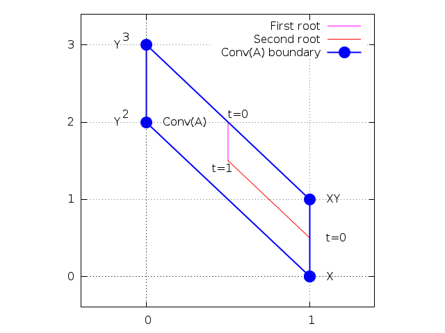
Figure 1. The momentum map for the two solutions of the running example between $t=1$ (center) and $t=0$ (on the boundary).

A particular choice of ${\mathbf{g}}\in(\mathbb{R}^{n})^{*}$ plays the rôle of the canonical basis in the $U(n+1)$-invariant homogeneous theory. This particular choice is related to an invariant of the toric action on $\mathbb{C}^{n}$: each $\theta\in(S^{1})^{n}=\mathbb{R}^{n}\bmod\mathbb{Z}^{n}$ maps $\mathbf{x}$ to $\mathbf{x}+2\pi\theta\sqrt{-1}$. The reproducing kernel $K(\mathbf{x},\mathbf{x})$ is invariant through this action, and the Hermitian metric happens to be equivariant. The momentum map associated to the toric action is

$$\begin{array}[]{lrcl}\mathbf{m}:&\mathbb{C}^{n}&\longrightarrow&\mathrm{Conv}(A)\subseteq(\mathbb{R}^{n})^{*}\\ &\mathbf{x}&\longmapsto&\mathbf{m}(\mathbf{x})=\frac{1}{2}D\log(K(\mathbf{x},\mathbf{x}))=\frac{1}{\|V(\mathbf{x})\|^{2}}V(\mathbf{x})^{*}DV(\mathbf{x})\end{array}.$$

At each point $\mathbf{x}$, the momentum map $\mathbf{m}(\mathbf{x})$ is also a convex linear combination of the points in $A$. Points at toric infinity map to points on the boundary of $\mathrm{Conv}(A)$ (Figure 1).

At a fixed point $\mathbf{x}_{0}\in\mathbb{C}^{n}$, we set $\mathbf{g}=\mathbf{m}{\stackrel{{\scriptstyle\mathrm{def}}}{{=}}}\mathbf{m}(\mathbf{x}_{0})$ and $W(\mathbf{x})\stackrel{{\scriptstyle\mathrm{def}}}{{=}}W_{\mathbf{m}}(\mathbf{x})=e^{-\mathbf{m}\mathbf{x}}V(\mathbf{x})$. The derivative of each $[V(\mathbf{x})]$ at $\mathbf{x}_{0}$ can be written in normalized coordinates as

$$\begin{array}[]{lrcl}D[V](\mathbf{x}_{0}):&T_{\mathbf{x}_{0}}\mathbb{C}^{n}&\longrightarrow&T_{[V(\mathbf{x}_{0})]}\mathscr{F}^{*}\\ &\dot{\mathbf{x}}&\longmapsto&\frac{1}{\|V(\mathbf{x}_{0})\|}\left(I-\frac{1}{\|V(\mathbf{x}_{0})\|^{2}}V(\mathbf{x}_{0})V(\mathbf{x}_{0})^{*}\right)DV(\mathbf{x}_{0})\dot{\mathbf{x}}\end{array}$$

while introducing $W=W_{\mathbf{m}}$ one has $W^{*}(\mathbf{x}_{0})DW(\mathbf{x}_{0})=0$ so

$$D[V](\mathbf{x}_{0})=D[W](\mathbf{x}_{0}):\dot{\mathbf{x}}\mapsto\frac{1}{\|W(\mathbf{x}_{0})\|}DW(\mathbf{x}_{0})\dot{\mathbf{x}}.$$

The Lemma below also allows us to assume without loss of generality that $\mathbf{m}(\mathbf{x}_{0})=0$ at some special point $\mathbf{x}_{0}$.

Lemma 3.2.2.

On a neighborhood of $\mathbf{x}_{0}$, define $\hat{\mathbf{m}}(\mathbf{x})=\frac{1}{\|W(\mathbf{x})\|^{2}}W^{*}(\mathbf{x})DW(\mathbf{x})$. Then $\hat{\mathbf{m}}(\mathbf{x})=\mathbf{m}(\mathbf{x})-\mathbf{m}(\mathbf{x}_{0})$.

Proof.

We use the formula $\mathbf{m}(\mathbf{x})=\frac{1}{2}D\log(K(\mathbf{x},\mathbf{x}))$. The reproducing kernel associated to $W$ is $K(\mathbf{x},\mathbf{x})e^{-2\mathbf{m}(\mathbf{x}_{0})\mathrm{Re}(\mathbf{x})}$ so $\hat{\mathbf{m}}(\mathbf{x})=\mathbf{m}(\mathbf{x})-\mathbf{m}(\mathbf{x}_{0})$. ∎

3.3. Systems of equations

From now on, we assume that each $\mathscr{F}_{i}=\mathscr{F}_{A_{i}}$ is a finite dimensional space of exponential sums over $\mathbb{C}^{n}$, with orthonormal basis

$$(\dots,\rho_{\mathbf{a}}e^{\mathbf{a}\mathbf{x}},\dots)_{\mathbf{a}\in A_{i}}$$

where the coefficients $\rho_{\mathbf{a}}>0$ are arbitrary. The evaluation map for each $\mathscr{F}_{i}$ will be denoted by $V_{i}$ and its reproducing kernel by $K_{i}(\mathbf{x},\mathbf{y})$. Let $\mathscr{V}_{0}\subset\mathbb{P}(\mathscr{F}_{1}^{*})\times\cdots\times\mathbb{P}(\mathscr{F}_{n}^{*})$ be the image of $\left[V\right]=\left(\left[V_{1}\right],\dots,\left[V_{n}\right]\right)$. Let $\mathscr{V}=\overline{\mathscr{V}}_{0}$ be the Zariski closure of $\mathscr{V}_{0}$. Points at $\mathscr{V}\setminus\mathscr{V}_{0}$ are said to be at toric infinity.

Let $\langle\cdot,\cdot\rangle_{\mathbf{x}}$ be the pull-back by $[V]$ at $x$ of the Fubini-Study Hermitian product on $\mathscr{V}_{0}\subset\mathbb{P}(\mathscr{F}_{1})\times\cdots\times\mathbb{P}(\mathscr{F}_{n})$. Namely,

$$\langle\cdot,\cdot\rangle_{\mathbf{x}}=\langle\cdot,\cdot\rangle_{1,\mathbf{x}}+\cdots+\langle\cdot,\cdot\rangle_{n,\mathbf{x}}$$

and $\langle\mathbf{u},\mathbf{u}\rangle_{i,\mathbf{x}}\leq\langle\mathbf{u},\mathbf{u}\rangle_{\mathbf{x}}$ for all $\mathbf{u}$, where $\langle\cdot,\cdot\rangle_{i,\mathbf{x}}$ and $\|\cdot\|_{i,\mathbf{x}}$ are the Hermitian inner product and norm associated to the $i$-th space $\mathscr{F}_{i}$. A metric structure on $\mathscr{V}$ is given by the induced norm for the Hermitian inner product,

$$\|\cdot\|_{\mathbf{x}}=\sqrt{\langle\cdot,\cdot\rangle_{\mathbf{x}}}.$$

This is not the only possibility. In Section 6 we replace this norm on $\mathcal{V}$ with the Finsler structure $\vvvert\cdot\vvvert=\max_{i}\|\cdot\|_{\mathbf{x},i}$.

It is convenient to parameterize $\mathscr{V}_{0}\subset\mathscr{V}$ through an isometric chart. Let $\mathbb{C}^{n}/[V]$ be the quotient obtained by identifying two points of $\mathbb{C}^{n}$ whenever they have the same image by $[V]$. Let $\mathscr{M}=(\mathbb{C}^{n}/[V],\langle\cdot,\cdot\rangle_{\mathbf{x}})$.

Lemma 3.3.1.

$\mathscr{M}$ is a Hermitian manifold, isometric to $\mathscr{V}_{0}$.

Proof.

Without loss of generality, assume that each $A_{i}\ni 0$. Let $N$ be the space of all $\mathbf{u}\in\mathbb{C}^{n}$ such that $\mathbf{a}\mathbf{u}=0$ for all $a\in A_{i}$, $i=1,\dots,n$. Let $W$ be such that $\mathbb{C}^{n}=N\oplus W$. Then $\mathbb{C}^{n}/[V]$ and $W/[V]$ are the same.

Two points $\mathbf{x}$ and $\mathbf{z}\in W$ share the same image by $[V]$ if and only if there are constants $c_{1},\dots,c_{n}\in\mathbb{C}$ so that for any $i$ and for any $\mathbf{a}\in A_{i}$,

$$e^{\mathbf{a}(\mathbf{x}-\mathbf{z})}=e^{c_{i}}.$$

For all $\mathbf{a}\in A_{i}$ we will have

$$\mathbf{a}(\mathbf{x}-\mathbf{z})\equiv c_{i}\mod 2\pi\sqrt{-1}$$

Since $0\in A_{i}$, we can take $c_{i}=0$.

By construction of $W$, there is a subset $\{\mathbf{a}_{1},\dots,\mathbf{a}_{r}\}$ of $\cup A_{i}$ that is a basis of $W$ as a complex vector space. Let $W_{\mathbb{R}}=\{\mathrm{Re}(u):u\in W\}$ be the real projection of $W$. Since the $\mathbf{a}_{j}$ are real vectors, the same subset of $\cup A_{i}$ is a basis of the real vector space $W_{\mathbb{R}}$. As a consequence

$$\Lambda=\left\{\mathbf{u}\in W:\mathbf{a}\mathbf{u}\equiv 0\mod 2\pi\right\}$$

is an $r$-dimensional lattice. As a topological space, $\mathcal{M}$ is the quotient of $W$ by the equivalence relation

$$\mathbf{x}\equiv\mathbf{y}\Leftrightarrow\mathbf{x}-\mathbf{y}=\mathbf{u}\sqrt{-1}\text{ for some }\mathbf{u}\in\Lambda.$$

Therefore $\mathscr{M}=W_{\mathbb{R}}\times W_{\mathbb{R}}/\Lambda$ is a smooth complex manifold of dimension $r$. The isometry property follows from the construction of the inner product. ∎

Remark 3.3.2.

Most theorems in this paper assume or imply the existence of nondegenerate roots, so that the mixed volume $V(\mathrm{Conv}(A_{1}),\dots,\mathrm{Conv}(A_{n}))$ does not vanish. In particular there is a mixed cell. Above, we can make this mixed cell to be in the form $[0,\mathbf{a}_{1}]\times\cdots\times[0,\mathbf{a}_{n}]$ so that $(\mathbf{a}_{1},\dots,\mathbf{a}_{n})$ is a basis for $W$ with $\mathbf{a}_{i}\in A_{i}$. In this case, $\mathscr{M}$ is a $n$-dimensional Hermitian manifold. See [Malajovich-Mixed] for details and references on mixed volume, mixed cells and such.

Remark 3.3.3.

The Lemma above can also be restated in terms of non-degenerate fewnomial spaces. If one of the $\mathcal{F}_{A_{i}}$ is non-degenerate and $0\in A_{i}$, then $A_{i}$ contains a basis for $\mathbb{R}^{n}$, etc…

Remark 3.3.4.

While $\mathscr{M}$ is also a smooth manifold, the closure $\mathscr{V}$ of $\mathscr{V}_{0}$ is not necessarily smooth. Just consider the span of $e^{3x}$, $e^{2x}$ and $1$. Then $\mathscr{V}$ is the projective curve $Y^{2}Z-X^{3}=0$ which has a singularity at $(0:0:1)$.

As in the previous section, a system $(f_{1},\dots,f_{n})\in\mathscr{F}_{1},\dots,\mathscr{F}_{n}$ does not have a well-defined value at some $([V(\mathbf{x})])$. Instead, it defines a section of the vector bundle $\pi:\mathscr{E}\rightarrow\mathbb{P}(\mathscr{F}_{1}^{*})\times\dots\times\mathbb{P}(\mathscr{F}_{n}^{*})$ with total space

$$\mathscr{E}=\left[(\mathscr{F}_{1}^{*}\setminus\{0\})\times\dots\times(\mathscr{F}_{n}^{*}\setminus\{0\})\times\mathbb{C}^{n}\right]$$

where the quotient is taken with respect to the ${\mathbb{C}_{\times}^{n}}$-action

$$\lambda(\mathbf{V},\mathbf{y})=(\lambda_{1}V_{1},\dots,\lambda_{n}V_{n},\lambda_{1}y_{1},\dots,\lambda_{n}y_{n}).$$

This bundle restricts to a vector bundle $\mathbb{C}^{n}\rightarrow\pi^{-1}(\mathscr{V}_{0})\subseteq\mathscr{E}\stackrel{{\scriptstyle\pi}}{{\rightarrow}}{\mathscr{V}_{0}}$, and pulls back to a bundle $\mathbb{C}^{n}\rightarrow\mathscr{E}_{0}=\pi^{-1}(\mathscr{V}_{0})\stackrel{{\scriptstyle[V]^{-1}\circ\pi}}{{\xrightarrow{\hskip 20.00003pt}}}{\mathscr{M}}$. The group $((\mathbb{R}^{n})^{*})^{n}$ acts coordinatewise on exponential sums: each $\mathbf{M}=(\mathbf{m}_{1},\dots,\mathbf{m}_{n})\in((\mathbb{R}^{n})^{*})^{n}$ maps $\mathscr{F}_{A_{1}}\times\cdots\times\mathscr{F}_{A_{n}}$ into $\mathscr{F}_{A_{1}-\mathbf{m}_{1}}\times\cdots\times\mathscr{F}_{A_{n}-\mathbf{m}_{n}}$.

To define a local trivialization, fix an arbitrary $\mathbf{x}_{0}\in\mathscr{M}$. Let $U_{0}=\{\mathbf{x}\in\mathscr{M}:V_{i}(\mathbf{x})\not\perp V_{i}(\mathbf{x}_{0})\}$. Also, let $\mathbf{m}_{i}=\mathbf{m}_{i}(\mathbf{x}_{0})$ be the momentum map at $\mathbf{x}_{0}$. Let $W_{i}(\mathbf{x})=e^{-\mathbf{m}_{i}(\mathbf{x}_{0})(\mathbf{x})}V_{i}(x)$. Then set

$$\begin{array}[]{lrcl}\phi_{\mathbf{x}_{0}}:&U_{0}\times\mathbb{C}^{n}&\longrightarrow&\mathscr{E}_{0}\\ &\mathbf{x},\mathbf{y}&\longmapsto&\left[W(\mathbf{x}),\mathbf{y}\right]\end{array}$$

To each $\mathbf{f}\in\mathscr{F}_{1}\times\cdots\times\mathscr{F}_{n}$ we associate the section

$$\begin{array}[]{lrcl}s_{\mathbf{f}}:&U_{0}\subseteq\mathscr{M}&\longrightarrow&\mathscr{E}_{0}\\ &\mathbf{x}_{0}+\dot{\mathbf{x}}&\longmapsto&\phi_{\mathbf{x}_{0}}(\mathbf{x}_{0}+\dot{\mathbf{x}},\mathbf{f}\cdot W(\mathbf{x}_{0}+\dot{\mathbf{x}}))\end{array}$$

where the notation $\mathbf{f}\cdot\mathbf{W}$ stands for the map $\mathscr{M}\rightarrow\mathbb{C}^{n}$ given by

$$\mathbf{f}\cdot\mathbf{W}=\begin{pmatrix}f_{1}\cdot W_{1}\\ \vdots\\ f_{n}\cdot W_{n}\end{pmatrix}\stackrel{{\scriptstyle\mathrm{def}}}{{=}}\begin{pmatrix}W_{1}(\mathbf{x})(f_{1})\\ \vdots\\ W_{n}(\mathbf{x})(f_{n})\end{pmatrix}.$$

The local function is now

$$\begin{array}[]{lrcl}S_{\mathbf{f},\mathbf{x}_{0}}:&U_{0}\subseteq T_{\mathbf{x}}\mathscr{M}&\longrightarrow&\mathbb{C}^{n}\\ &\dot{\mathbf{x}}&\longmapsto&\pi\circ\phi_{\mathbf{x}_{0}}^{-1}\left(\left[\mathbf{W}(\mathbf{x}_{0}+\dot{\mathbf{x}}),\mathbf{f}\cdot\mathbf{W}(\mathbf{x}_{0}+\dot{\mathbf{x}})\right]\right)\end{array}$$

where $\pi_{2}$ is the projection onto the second coordinate. In normalized coordinates,

(4) $$S_{\mathbf{f},\mathbf{x}_{0}}(\dot{\mathbf{x}})=\begin{bmatrix}f_{1}\cdot\left(\frac{1}{\|W_{1}(\mathbf{x}_{0})\|}W_{1}(\mathbf{x}_{0}+\dot{\mathbf{x}})\right)\\ \vdots\\ f_{n}\cdot\left(\frac{1}{\|W_{n}(\mathbf{x}_{0})\|}W_{n}(\mathbf{x}_{0}+\dot{\mathbf{x}})\right)\end{bmatrix}$$

The local Newton operator is

$$\begin{array}[]{lrcl}{\mathbf{N}}_{\mathbf{f},\mathbf{x}_{0}}:&T_{\mathbf{x}_{0}}\mathscr{M}&\longrightarrow&T_{x_{0}}\mathscr{M}\\ &\dot{\mathbf{x}}&\longmapsto&\dot{\mathbf{x}}-DS_{\mathbf{f},\mathbf{x}_{0}}(\dot{\mathbf{x}})^{-1}S_{\mathbf{f},\mathbf{x}_{0}}(\dot{\mathbf{x}})\end{array}.$$

In order to define a global Newton operator, one needs a map from $T\mathscr{M}$ onto $\mathscr{M}$. We will use the sum from $\mathbb{C}^{n}$. The map $(\mathbf{x}_{0},\dot{\mathbf{x}})\mapsto\mathbf{x}_{0}+\dot{\mathbf{x}}$ is the parallel transport associated to the trivial (zero) connection on $\mathscr{M}$. The global Newton operator on $\mathscr{M}$ using that map is

$$\begin{array}[]{lrcl}{\mathbf{N}}_{\mathbf{f}}:&\mathscr{M}&\longrightarrow&\mathscr{M}\\ &\mathbf{x}_{0}&\longmapsto&\mathbf{x}_{0}+{\mathbf{N}}_{\mathbf{f},\mathbf{x}_{0}}(0).\end{array}$$

If ${\mathbf{N}}_{\mathbf{f}}(\mathbf{x}_{0})\not\in\mathscr{M}$ we say that ${\mathbf{N}}_{\mathbf{f}}(\mathbf{x}_{0})$ is not defined.

The group $((\mathbb{R}^{n})^{*})^{n}$ acts coordinatewise on exponential sums: each $\mathbf{M}=(\mathbf{m}_{1},$ $\dots,\mathbf{m}_{n})\in((\mathbb{R}^{n})^{*})^{n}$ maps $\mathscr{F}_{A_{1}}\times\cdots\times\mathscr{F}_{A_{n}}$ into $\mathscr{F}_{A_{1}-\mathbf{m}_{1}}\times\cdots\times\mathscr{F}_{A_{n}-\mathbf{m}_{n}}$. If we are given some $\mathbf{x}_{0}\in\mathscr{M}$, we can always assume without loss of generality that $\mathbf{m}_{i}(\mathbf{x}_{0})=0$ for all $i$. This simplifies the formulas for $\mathbf{V}$, $S_{\mathbf{f},\mathbf{x}_{0}}$ and derivatives. For instance,

$$DS_{\mathbf{f},\mathbf{x}_{0}}(0)=\begin{bmatrix}f_{1}\cdot\left(\frac{1}{\|V_{1}(\mathbf{x}_{0})\|}DV_{1}(\mathbf{x}_{0})\right)\\ \vdots\\ f_{n}\cdot\left(\frac{1}{\|V_{n}(\mathbf{x}_{0})\|}DV_{n}(\mathbf{x}_{0})\right)\end{bmatrix}.$$

3.4. Condition number theory

Assume now that $\mathbf{m}(\mathbf{x}_{0})=0$, $\mathbf{f}\cdot\mathbf{V}(\mathbf{x}_{0})=0$ and $DS_{\mathbf{f}_{0},\mathbf{x}_{0}}$ is non-degenerate. The implicit function theorem asserts that there is a smooth function $G:U\subseteq\mathbb{P}(\mathscr{F}_{1})\times\cdots\times\mathbb{P}(\mathscr{F}_{n})\rightarrow\mathscr{M}$ with $\mathbf{f}\cdot\mathbf{V}(G(\mathbf{f}))\equiv 0$, defined on a neighborhood $U\ni\mathbf{f}_{0}$. Its derivative at $\mathbf{f}_{0}$ is

$$DG(\mathbf{f}_{0})\dot{\mathbf{f}}=DS_{\mathbf{f}_{0},\mathbf{x}_{0}}(0)^{-1}\dot{\mathbf{f}}(\mathbf{x}).$$

Using the reproducing kernel notation and assuming $\dot{\mathbf{f}}_{i}\perp f_{i}$,

$$DG(\mathbf{f}_{0})\dot{\mathbf{f}}=DS_{\mathbf{f}_{0},\mathbf{x}_{0}}(0)^{-1}\frac{\|f_{1}\|}{\|K_{1}(\cdot,\mathbf{x})\|}K_{1}(\cdot,\mathbf{x})^{*}\oplus\cdots\oplus\frac{\|f_{n}\|}{\|K_{n}(\cdot,\mathbf{x})\|}K_{n}(\cdot,\mathbf{x})^{*}.$$

This motivates the following definition:

Definition 3.4.1.

The toric condition number of $\mathbf{f}$ at $\mathbf{x}$ is

$$\mu(\mathbf{f},\mathbf{x})=\|DG(\mathbf{f})\|_{\mathbf{x}}=\left\|DS_{\mathbf{f},\mathbf{x}}(0)^{-1}\begin{pmatrix}\|f_{1}\|\\ &\ddots\\ &&\|f_{n}\|\end{pmatrix}\right\|_{\mathbf{x}}$$

where the operator norm from $\mathbb{C}^{n}$ (with canonical inner product) into $(\mathscr{M},\|\cdot\|_{\mathbf{x}})$ is assumed.

The condition number is invariant through scaling of each of the $f_{i}$. Therefore we also write $\mu([\mathbf{f}],\mathbf{x})=\mu(\mathbf{f},\mathbf{x})$. Notice that because of the normalization,

(5) $$\mu(\mathbf{f},\mathbf{x})\geq 1$$

always.

A condition number theorem for $\mu(\mathbf{f},\mathbf{x})$ in terms of inverse distances is known. In the language of this paper, it reads:

Theorem 3.4.2.

[Malajovich-Rojas]*Th.4 Let $\Sigma_{\mathbf{x}}=\{\mathbf{f}:S_{\mathbf{f},\mathbf{x}}(0)=0\text{ and }\det{DS_{\mathbf{f},\mathbf{x}}(0)}=0\}$. Then,

$$\max_{\|\dot{\mathbf{f}}\|\leq\|\mathbf{f}\|}\min_{i}\left\|DG(\mathbf{f})\dot{\mathbf{f}}\right\|_{i,\mathbf{x}}\leq d_{P}(\mathbf{f},\Sigma_{\mathbf{x}})^{-1}\leq\mu(\mathbf{f},\mathbf{x})$$

where $d_{P}$ is the projective (sine) metric.

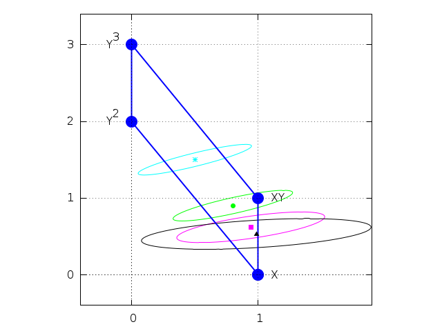
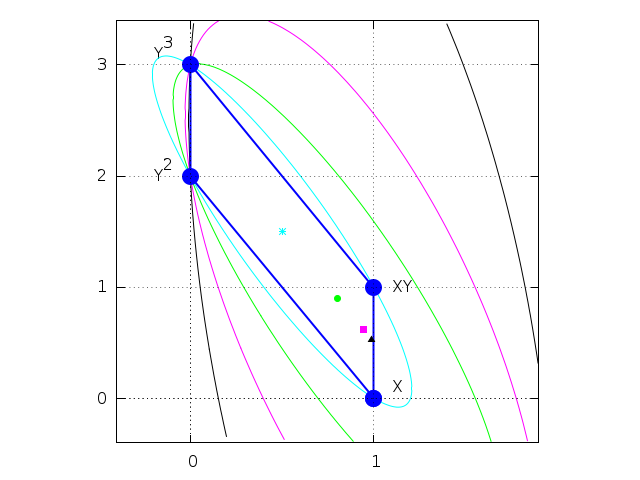
Figure 2. Left: Unit circles for the Hermitian metric $\langle\cdot,\cdot\rangle_{i,\mathbf{x}}$ from the running example, at several points. The circles are centered at $\mathbf{m}_{i}(\mathbf{x})$ and shrinked by a factor of 10 to fit in the picture. Right: radius $\nu_{i}$ circles of the dual metric. Both pictures are independent of the value of $i$.

The condition numbers $\nu_{i}(\mathbf{x})$ defined below play an important rôle in this paper.

Definition 3.4.3.

The $\|\cdot\|_{i,\mathbf{x}}$ – circumscribed radius of $\mathrm{Conv}(A_{i}-\mathbf{m}_{i}(\mathbf{x}))$ is

$$\nu_{i}(\mathbf{x})=\max_{\mathbf{a}\in A_{i}}\sup_{\|\mathbf{u}\|_{i,\mathbf{x}}\leq 1}|(\mathbf{a}-\mathbf{m}_{i}(\mathbf{x}))\mathbf{u}|.$$

Also, we set

$$\nu(\mathbf{x})=\max_{i}\nu_{i}(\mathbf{x})$$

Figure 2 shows the unit balls $\|\mathbf{u}\|_{i,\mathbf{x}}\leq 1$ from the running example at a few points. It also shows the radius $\nu_{i}(\mathbf{x})$-balls from the dual metric.

Remark 3.4.4.

There is no guarantee that the unit ball for a $\|\cdot\|_{i,\mathbf{x}}$ is compact. If $\mathrm{Span}(\mathbf{a}-\mathbf{m}_{i}(\mathbf{x}))$ is a proper subspace of $\mathbb{R}^{n}$, then any vector $\mathbf{u}$ can be decomposed as $\mathbf{u}=\mathbf{u}_{1}+\mathbf{u}_{2}$ with $\mathbf{u}_{1}\in\mathrm{Span}(\mathbf{a}-\mathbf{m}_{i}(\mathbf{x}))$ and $\mathbf{u}_{2}\perp\mathrm{Span}(\mathbf{a}-\mathbf{m}_{i}(\mathbf{x}))$. In that case $\|\mathbf{u}\|_{i,\mathbf{x}}=\|\mathbf{u}_{1}\|_{i,\mathbf{x}}$ and $(\mathbf{a}-\mathbf{m}_{i}(\mathbf{x}))\mathbf{u}=(\mathbf{a}-\mathbf{m}_{i}(\mathbf{x}))\mathbf{u}_{1}$.

The reader should check that $1\leq\nu_{i}(\mathbf{x})$ and that

(6) $$\max_{\mathbf{a}\in A_{i}}\sup_{\|\mathbf{u}\|_{\mathbf{x}}\leq 1}|(\mathbf{a}-\mathbf{m}_{i}(\mathbf{x}))\mathbf{u}|\leq\nu_{i}(\mathbf{x})\leq\nu(\mathbf{x}).$$

As mentioned before, we are avoiding to use geodesics and parallel transport to move from one point to another. Instead, we use the trivial transport operator $\mathbf{u}\in T_{\mathbf{x}}\mathscr{M}\mapsto\mathbf{u}\in T_{\mathbf{y}}\mathscr{M}$. This operator is not isometric, but the distortion it introduces can be bounded in terms of $\nu(\mathbf{x})$:

Lemma 3.4.5.

Let $s=\nu(\mathbf{x})\|\mathbf{y}-\mathbf{x}\|_{\mathbf{x}}$. Then for all $i$,

$$(2-e^{s})\|\mathbf{u}\|_{i,\mathbf{x}}\leq\|\mathbf{u}\|_{i,\mathbf{y}}\leq e^{s}\|u\|_{i,\mathbf{x}}.$$

Moreover,

$$(2-e^{s})\|\mathbf{u}\|_{\mathbf{x}}\leq\|\mathbf{u}\|_{\mathbf{y}}\leq e^{s}\|\mathbf{u}\|_{\mathbf{x}}.$$

The exponential bounds above are not as inconvenient as they look. Typically, $s$ is small. If $s<1$, $1+s\leq e^{s}<1/(1-s)$.

One of the main tools in recent homotopy papers such as [Bezout6, Bezout7, Adaptive, Burgisser-Cucker] is an estimate on the sensitivity of the condition number. In this paper we will use the following bound instead:

Theorem 3.4.6.

Assume that $\theta=(\|\mathbf{x}-\mathbf{y}\|_{\mathbf{x}}+d_{P}([\mathbf{f}],[\mathbf{g}]))\mu(\mathbf{f},\mathbf{x})\nu(\mathbf{x})<1/5$. Then,

$$\mu(\mathbf{f},\mathbf{x})\nu(\mathbf{x})(1-5\theta)\leq\mu(\mathbf{g},\mathbf{y})\nu(\mathbf{y})\leq\frac{\mu(\mathbf{f},\mathbf{x})\nu(\mathbf{x})}{1-5\theta}.$$

where $d_{P}$ is the multiprojective (sine) distance.

The multiprojective distance is defined by

$$d_{P}([\mathbf{f}],[\mathbf{g}])^{2}=\sum_{i}\inf_{\lambda\in\mathbb{C}}\frac{\|\mathbf{f}_{i}-\lambda\mathbf{g}_{i}\|^{2}}{\|\mathbf{f}_{i}\|^{2}}.$$

In the definition of $\theta$, the multiprojective distance can be replaced by the Riemannian distance which is larger.

3.5. Quadratic convergence

The invariants for the toric Newton operator are:

$$\beta(\mathbf{f},\mathbf{x})\stackrel{{\scriptstyle\mathrm{def}}}{{=}}\|{\mathbf{N}}_{\mathbf{f}}(\mathbf{x})-\mathbf{x}\|_{\mathbf{x}}=\|DS_{\mathbf{f},\mathbf{x}}(0)^{-1}S_{\mathbf{f},\mathbf{x}}(0)\|_{\mathbf{x}},$$

$$\gamma(\mathbf{f},\mathbf{x})\stackrel{{\scriptstyle\mathrm{def}}}{{=}}\max_{k\geq 2}\left(\frac{1}{k!}\left\|DS_{\mathbf{f},\mathbf{x}}(0)^{-1}D^{k}S_{\mathbf{f},\mathbf{x}}(0)\right\|_{\mathbf{x}}\right)^{1/(k-1)}$$

and of course $\alpha(\mathbf{f},\mathbf{x})=\beta(\mathbf{f},\mathbf{x})\gamma(\mathbf{f},\mathbf{x})$.

We assume that $\mathbf{z}$ is a non-degenerate zero of the line bundle section given by $\mathbf{f}$. All norms will be taken with respect to $T_{\mathbf{z}}\mathscr{M}$.

Theorem 3.5.1 ($\gamma$-theorem).

Let $\mathbf{z}\in\mathscr{M}$ be a non-degenerate zero of $\mathbf{f}$. If $\mathbf{x}_{0}\in\mathscr{M}$ satisfies

$$\|\mathbf{x}_{0}-\mathbf{z}\|_{\mathbf{z}}\left(\gamma(\mathbf{f},\mathbf{z})+\mu(\mathbf{f},\mathbf{z})\max_{i}\sup_{\|\mathbf{u}\|_{\mathbf{z}}\leq 1}|(\mathbf{m}_{i}(\mathbf{z})-\mathbf{m}_{i}(\mathbf{x}))\mathbf{u}|\right)\leq\frac{3-\sqrt{7}}{2},$$

then the sequence $\mathbf{x}_{i+1}={\mathbf{N}}_{\mathbf{f}}(\mathbf{x}_{i})$ is well-defined and

$$\|\mathbf{x}_{i}-\mathbf{z}\|_{\mathbf{z}}\leq 2^{-2^{i}+1}\|\mathbf{x}_{0}-\mathbf{z}\|_{\mathbf{z}}.$$

A trivial bound for $\sup_{\|\mathbf{u}\|_{\mathbf{z}}\leq 1}|(\mathbf{m}_{i}(\mathbf{z})-\mathbf{m}_{i}(\mathbf{x}))\mathbf{u}|$ is the circumscribed radius $\nu_{i}(\mathbf{z})$. We will obtain a sharper bound in Theorem 4.1.1. Theorem 3.5.1 is proved in Section 5.1.

Theorem 3.5.2 ($\alpha$-theorem).

Let

$$\alpha\leq\alpha_{0}=\frac{13-3\sqrt{17}}{4}.$$

Let

$$r_{0}=\frac{1+\alpha-\sqrt{1-6\alpha+\alpha^{2}}}{4\alpha}\text{ and }r_{1}=\frac{1-3\alpha-\sqrt{1-6\alpha+\alpha^{2}}}{4\alpha}.$$

If $\mathbf{x}_{0}\in\mathscr{M}$ satisfies $\alpha(\mathbf{f},\mathbf{x}_{0})\leq\alpha$, then the sequence defined recursively by $\mathbf{x}_{i+1}=\mathbf{x}_{0}+{\mathbf{N}}_{\mathbf{f},\mathbf{x}_{0}}(\mathbf{x}_{i}-\mathbf{x}_{0})$ is well-defined and converges to a zero $\boldsymbol{\zeta}\in\mathscr{M}$ of $f$. Furthermore,

1. $\|\mathbf{x}_{i}-\boldsymbol{\zeta}\|_{\mathbf{x}_{0}}\leq 2^{-2^{i}+1}\|\mathbf{x}_{1}-\mathbf{x}_{0}\|_{\mathbf{x}_{0}}$

2. $\|\mathbf{x}_{i}-\boldsymbol{\zeta}\|_{\boldsymbol{\zeta}}\leq 2^{-2^{i}+1}\|\mathbf{x}_{1}-\mathbf{x}_{0}\|_{\mathbf{x}_{0}}$

3. $\|\mathbf{x}_{0}-\boldsymbol{\zeta}\|_{\mathbf{x}_{0}}\leq r_{0}\beta(\mathbf{f},\left[\mathbf{x}_{0}\right])$

4. $\|\mathbf{x}_{0}-\boldsymbol{\zeta}\|_{\boldsymbol{\zeta}}\leq r_{0}\beta(\mathbf{f},\left[\mathbf{x}_{0}\right])$

5. $\|\mathbf{x}_{1}-\boldsymbol{\zeta}\|_{\boldsymbol{\zeta}}\leq r_{1}\beta(\mathbf{f},\left[\mathbf{x}_{0}\right]).$

Proof.

Items (a) and (c) are just Theorem 2.1.2(a,c) applied to $S_{\mathbf{f},\mathbf{x}_{0}}:T_{\mathbf{x}_{0}}\mathscr{M}=T_{\mathbf{V}(\mathbf{x}_{0})}\mathscr{V}\rightarrow\mathbb{C}^{n}$. The proof of item (b) mimics the proof of Theorem 2.5.2(b). For all $1\leq j\leq n$, we claim that

(7) $$\|\dot{\mathbf{x}}_{i}\|_{j,\mathbf{x}}\leq 2^{-2^{i}+1}\|\dot{\mathbf{x}}^{*}\|_{j,\mathbf{x}}.$$

Indeed, assume without loss of generality that $\mathbf{m}_{j}(\mathbf{x})=0$. Then we set $v_{j}(\mathbf{x})=\frac{1}{V_{j}(\mathbf{x})}V_{j}(\mathbf{x})$, so that

$$Dv_{j}(\mathbf{x})=\frac{1}{V_{j}(\mathbf{x})}DV_{j}(\mathbf{x}).$$

By definition, $\|\mathbf{u}\|_{j,\mathbf{x}}=\|Dv_{j}(\mathbf{x})\mathbf{u}\|$. Moreover, $Dv_{j}(\mathbf{x})\mathbf{u}\perp v_{j}(\mathbf{x})$. Let $\mathbf{X}=v_{j}(\mathbf{x}_{0})$, $\mathbf{Y}=v_{j}(\mathbf{x}_{0})+Dv_{j}(\mathbf{x}_{0})\dot{\mathbf{x}}_{i}$ and $Z=Dv_{j}(\mathbf{x}_{0})\dot{\mathbf{x}}^{*}$. By item (a), $\|Y-Z\|\leq\|X-Z\|$. Therefore, Lemma 2.5.3 implies that

$$\frac{\|\pi(Y)-Z\|}{\|Z\|}\leq\frac{\|Y-Z\|}{\|X\|}\leq 2^{-2^{i}+1}\frac{\|X-Z\|}{\|X\|}$$

where $\pi$ is the projection onto $Z+Z^{\perp}$. This establishes equation (7). Squaring, adding for all $j$ and taking square roots, one gets:

$$\|\dot{\mathbf{x}}_{i}\|_{\mathbf{x}}\leq 2^{-2^{i}+1}\|\dot{\mathbf{x}}^{*}\|_{\mathbf{x}}$$

The proof of items (d) and (e) is similar. ∎

3.6. The higher derivative estimate

A most important bound in modern homotopy papers is the higher derivative estimate. While $\gamma$ is an awkward invariant to approximate, there is a convenient upper bound:

Theorem 3.6.1.

$$\gamma(\mathbf{f},\mathbf{x})\leq\frac{1}{2}\mu(\mathbf{f},\mathbf{x})\nu(\mathbf{x})$$

This can be compared to the classical bound $\gamma_{0}(\mathbf{f},\boldsymbol{\zeta})\leq\frac{D^{3/2}}{2}\mu_{\text{norm}}(\mathbf{f},\boldsymbol{\zeta})$ for a homogeneous degree $D$ polynomial system and $\boldsymbol{\zeta}\in\mathbb{P}^{n}$, see for instance BCSS*Th. 2 Sec.14.2 or Burgisser-Cucker*Prop. 16.45. With some further work, we will recover a more convenient version of Theorem 3.5.1:

Theorem 3.6.2.

There is a constant $u_{0}\simeq 0.090994609\cdots$ with the following property. Let $\mathbf{z}\in\mathscr{M}$ be a non-degenerate zero of $\mathbf{f}$. If $\mathbf{x}_{0}\in\mathscr{M}$ satisfies

$$\frac{1}{2}\|\mathbf{x}_{0}-\mathbf{z}\|_{\mathbf{z}}\mu(\mathbf{f},\mathbf{z})\nu(\mathbf{z})\leq u_{0}$$

then the sequence $\mathbf{x}_{i+1}={\mathbf{N}}_{\mathbf{f}}(\mathbf{x}_{i})$ is well-defined and

$$\|\mathbf{x}_{i}-\mathbf{z}\|_{\mathbf{z}}\leq 2^{-2^{i}+1}\|\mathbf{x}_{0}-\mathbf{z}\|_{\mathbf{z}}.$$

Theorem 3.5.2 immediately becomes:

Theorem 3.6.3.

Let

$$\alpha\leq\alpha_{0}=\frac{13-3\sqrt{17}}{4}.$$

Let

$$r_{0}=\frac{1+\alpha-\sqrt{1-6\alpha+\alpha^{2}}}{4\alpha}\text{ and }r_{1}=\frac{1-3\alpha-\sqrt{1-6\alpha+\alpha^{2}}}{4\alpha}.$$

If $\mathbf{x}_{0}\in\mathscr{M}$ satisfies $\frac{1}{2}\beta(\mathbf{f},\mathbf{x}_{0})\mu(\mathbf{f},\mathbf{x}_{0})\nu(\mathbf{x}_{0})\leq\alpha$, then the sequence defined recursively by $\mathbf{x}_{i+1}=\mathbf{x}_{0}+{\mathbf{N}}_{\mathbf{f},\mathbf{x}_{0}}(\mathbf{x}_{i}-\mathbf{x}_{0})$ is well-defined and converges to a zero $\boldsymbol{\zeta}\in\mathscr{M}$ of $\mathbf{f}$. Furthermore,

1. $\|\mathbf{x}_{i}-\boldsymbol{\zeta}\|_{\mathbf{x}_{0}}\leq 2^{-2^{i}+1}\|\mathbf{x}_{1}-\mathbf{x}_{0}\|_{\mathbf{x}_{0}}$.

2. $\|\mathbf{x}_{i}-\boldsymbol{\zeta}\|_{\boldsymbol{\zeta}}\leq 2^{-2^{i}+1}\|\mathbf{x}_{1}-\mathbf{x}_{0}\|_{\mathbf{x}_{0}}$

3. $\|\mathbf{x}_{0}-\boldsymbol{\zeta}\|_{\mathbf{x}_{0}}\leq r_{0}\beta(\mathbf{f},\mathbf{x}_{0})$

4. $\|\mathbf{x}_{1}-\boldsymbol{\zeta}\|_{\boldsymbol{\zeta}}\leq r_{1}\beta(\mathbf{f},\mathbf{x}_{0}).$

Corollary 3.6.4.

There is a constant $\alpha_{1}\simeq 0.081239483\cdots$ with the following properties: If

$$\frac{1}{2}\mu(\mathbf{f},\mathbf{x}_{0})\nu(\mathbf{x}_{0})\beta(\mathbf{x}_{0})\leq\alpha\leq\alpha_{1},$$

then the sequence $\mathbf{x}_{i+1}={\mathbf{N}}_{\mathbf{f}}(\mathbf{x}_{i})$ is well defined, converges to a zero $\mathbf{z}$ of $\mathbf{f}$, and furthermore

$$\|\mathbf{x}_{i}-\mathbf{z}\|_{\mathbf{z}}\leq 2^{-2^{i-1}+1}r_{1}(\alpha)\beta(\mathbf{f},\mathbf{x}_{0}).$$

When $\alpha=\alpha_{1}$, $r_{1}(\alpha)\simeq 0.110020136\cdots$.

Proof.

Let $\alpha_{1}$ be the smallest positive root of

$$\frac{\alpha r_{1}(\alpha)}{1-10\alpha r_{0}(\alpha)}=u_{0}$$

where $u_{0}\simeq 0.090094609\cdots$ is the constant from Theorem 3.6.2. From Theorem 3.5.2(e), there is a zero $\mathbf{z}$ of $\mathbf{f}$ such that

$$\|\mathbf{x}_{1}-\mathbf{z}\|_{\mathbf{z}}\leq r_{1}(\alpha)\beta(\mathbf{f},\mathbf{x}_{0}).$$

Combining this with Theorem 3.4.6,

$$\frac{1}{2}\mu(\mathbf{f},\mathbf{z})\nu(\mathbf{z})\|\mathbf{x}_{1}-\mathbf{z}\|_{\mathbf{z}}\leq\frac{\alpha r_{1}(\alpha)}{1-10\alpha r_{0}(\alpha)}=u_{0}.$$

From Theorem 3.6.2, the rest of the sequence $\mathbf{x}_{i+1}={\mathbf{N}}_{\mathbf{f}}(\mathbf{x}_{i})$ is well defined, converges to $\mathbf{z}$ and

$$\|\mathbf{x}_{i}-\mathbf{z}\|_{\mathbf{z}}\leq 2^{-2^{i-1}+1}\|\mathbf{x}_{1}-\mathbf{x}_{2}\|\leq 2^{-2^{i-1}+1}r_{1}(\alpha)\beta(\mathbf{f},\mathbf{x}_{0}).$$

∎

Corollary 3.6.5.

Let $(\mathbf{f}_{t})_{t\in[0,T]}$ be a $\mathcal{C}^{1}$ path in $\mathbb{P}(\mathscr{F}_{1})\times\cdots\times\mathbb{P}(\mathscr{F}_{n})$. Assume that the point $\mathbf{x}_{0}$ satisfies, for all $t\in[0,T]$, that $\frac{1}{2}\mu(\mathbf{f}_{t},\mathbf{x})\nu(\mathbf{f}_{t},\mathbf{x}_{t})\beta(\mathbf{f}_{t},\mathbf{x}_{t})\leq\alpha<4/45=0.0888\cdots$. Then for each $t\in[0,T]$, the sequence $\mathbf{x}_{0}(t)=\mathbf{x}_{0}$, $\mathbf{x}_{i+1}(t)=\mathbf{x}_{0}+{\mathbf{N}}_{\mathbf{f}_{t},\mathbf{x}_{0}}(\mathbf{x}_{i}(t)-\mathbf{x}_{0})$ converges uniformly to some $\mathcal{C}^{1}$ path $\boldsymbol{\zeta}(t)$,

Proof.

By hypothesis $\mu(\mathbf{f}_{t},\mathbf{x}_{0})$ is bounded for $t\in[0,T]$. Hence $\mu(\mathbf{f}_{t},\mathbf{x}_{0})\leq\bar{\mu}$ for some finite $\bar{\mu}$. By Th. 3.6.3(c), $u=\mu(\mathbf{f}_{t},\mathbf{x}_{0})\nu(\mathbf{f}_{t},\mathbf{x}_{0})\|\mathbf{x}_{0}-\boldsymbol{\zeta}\|_{\mathbf{x}_{0}}\leq 2r_{0}(\alpha)\alpha<1/5$. Thus, $\mu(\mathbf{f}_{t},\boldsymbol{\zeta}(t))\leq\bar{\mu}/(1-5u)$ is finite. By construction of the condition number,

$$\left\|\frac{\partial}{\partial t}\boldsymbol{\zeta}(t)\right\|_{\boldsymbol{\zeta}(t)}\leq\frac{\bar{\mu}}{1-5u}\left\|\frac{\partial}{\partial t}[\mathbf{f}_{t}]\right\|_{[\mathbf{f}(t)]}$$

which is finite by compactness of the path $(\mathbf{f}_{t})_{t\in[0,T]}$. ∎

3.7. The cost of homotopy

Recall that the solution variety is

$$\mathscr{S}_{0}=\left\{\rule{0.0pt}{12.91663pt}(\mathbf{f},\mathbf{z})\in\mathbb{P}(\mathscr{F}_{A_{1}})\times\cdots\times\mathbb{P}(\mathscr{F}_{A_{n}})\times\mathscr{M}:\mathbf{f}(\mathbf{z})=0\right\}$$

and that $\Sigma^{\prime}$ is the set where $\mu(\mathbf{f},\mathbf{x})\nu(\mathbf{x})=\infty$. The condition length was defined as

$$\mathscr{L}((\mathbf{f}_{t},\mathbf{z}_{t}):t_{0},t_{1})=\int_{t_{0}}^{t_{1}}\mu(\mathbf{f}_{t},\mathbf{z}_{t})\nu(\mathbf{z}_{t})\sqrt{\|\dot{\mathbf{f}}_{t}\|_{f_{t}}^{2}+\|\dot{\mathbf{z}}_{t}\|_{\mathbf{z}_{t}}^{2}}\ \,\mathrm{d}t.$$

We will need below the auxiliary quantity

$$\mathscr{L}_{1}((\mathbf{f}_{t},\mathbf{z}_{t}):t_{0},t_{1})=\int_{t_{0}}^{t_{1}}\mu(\mathbf{f}_{t},\mathbf{z}_{t})\nu(\mathbf{z}_{t})\left(\|\dot{\mathbf{f}}_{t}\|_{f_{t}}+\|\dot{\mathbf{z}}_{t}\|_{\mathbf{z}_{t}}\right)\ \,\mathrm{d}t.$$

that relates to the condition length by

$$\mathscr{L}((\mathbf{f}_{t},\mathbf{z}_{t}):t_{0},t_{1})\leq\mathscr{L}_{1}((\mathbf{f}_{t},\mathbf{z}_{t}):t_{0},t_{1})\leq\sqrt{2}\mathscr{L}((\mathbf{f}_{t},\mathbf{z}_{t}):t_{0},t_{1})$$

Proof of Main Theorem A.

Assume that $0<u\leq u_{0}=\frac{3-\sqrt{7}}{2}$ is given. Set $t_{0}=0$ and for $i=0,\dots,N-2$ choose $t_{i+1}$ so that ${\mathscr{L}_{1}(t_{i},t_{i+1})}=\delta$ for some constant $\delta$ to be determined. Then set $t_{N}=T$, and $\mathscr{L}(t_{N-1},t_{N})\leq\delta$.

We consider the following induction hypothesis:

(8) $$\frac{1}{2}\mu(\mathbf{f}_{t_{i}},\mathbf{z}_{t_{i}})\nu(\mathbf{z}_{t_{i}})\|\mathbf{z}_{t_{i}}-\mathbf{x}_{i}\|_{\mathbf{z}_{t_{i}}}\leq u$$

which is already satisfied for $i=0$. Theorem 3.6.2 implies that $\mathbf{x}_{i+1}={\mathbf{N}}(\mathbf{f}_{t_{i}},\mathbf{x}_{i})$ satisfies:

$$\frac{1}{2}\mu(\mathbf{f}_{t_{i}},\mathbf{z}_{t_{i}})\nu(\mathbf{z}_{t_{i}})\|\mathbf{z}_{t_{i}}-\mathbf{x}_{i+1}\|_{\mathbf{z}_{t_{i}}}\leq u/2$$

To simplify notations, let $\mu=\mu(\mathbf{f}_{t_{i}},\mathbf{z}_{t_{i}})$, $\nu=\nu(\mathbf{z}_{t_{i}})$, $\mu^{\prime}=\mu(\mathbf{f}_{t_{i+1}},\mathbf{z}_{t_{i+1}})$ and $\nu^{\prime}=\nu(\mathbf{z}_{t_{i+1}})$. Let $r=\max_{t_{i}\leq t\leq t_{i+1}}d_{S}(\mathbf{f}_{t},\mathbf{f}_{t_{i}})+\|\mathbf{z}_{t}-\mathbf{z}_{t_{i}}\|_{\mathbf{z}_{t_{i}}}$. Assume that the maximum is attained for $t=t^{*}$, $t_{i}\leq t^{*}\leq t_{i+1}$. Then,

$$\mu\ \nu\ r \leq \mu\ \nu\int_{t_{i}}^{t^{*}}\left\|\frac{\partial}{\partial t}[\mathbf{f}_{t}]\right\|_{[\mathbf{f}_{t}]}+\left\|\frac{\partial}{\partial t}z_{t}\right\|_{\mathbf{z}_{t}}\,\mathrm{d}t$$

$$\leq \frac{1}{1-5\mu\nu r}{\mathscr{L}_{1}(t_{i},t^{*})}$$

$$\leq \frac{1}{1-5\mu\nu r}{\mathscr{L}_{1}(t_{i},t_{i+1})}$$

Hence,

$$\mu\nu r(1-5\mu\nu r)\leq\delta.$$

The largest possible value of $\mu\nu r$ should therefore satisfiy the quadratic equation $\mu\nu r(1-5\mu\nu r)=\delta$. Solving the equation, we deduce that

$$\mu\nu r\leq R(\delta)\stackrel{{\scriptstyle\mathrm{def}}}{{=}}\frac{1}{10}\left(1-\sqrt{1-20\delta}\right)=\delta(1+o(1)).$$

Now we bound

$$\frac{1}{2}\mu^{\prime}\nu^{\prime}\|\mathbf{x}_{t_{i+1}}-\mathbf{z}_{t_{i+1}}\|_{\mathbf{z}_{t_{i}}} \leq \frac{1}{2}\mu^{\prime}\nu^{\prime}\left(\|\mathbf{x}_{t_{i+1}}-\mathbf{z}_{t_{i}}\|_{\mathbf{z}_{t_{i}}}+\|\mathbf{z}_{t_{i+1}}-\mathbf{z}_{t_{i}}\|_{\mathbf{z}_{t_{i}}}\right)$$

$$\leq \frac{1}{1-5\delta}\left(\frac{u}{2}+\frac{R(\delta)}{2}\right)$$

and from Lemma 3.4.5,

$$\frac{1}{2}\mu^{\prime}\nu^{\prime}\|\mathbf{x}_{t_{i+1}}-\mathbf{z}_{t_{i+1}}\|_{\mathbf{z}_{t_{i+1}}}\leq\frac{e^{R(\delta)}}{1-5\delta}\left(\frac{u}{2}+\frac{R(\delta)}{2}\right)$$

The induction hypothesis (8) is guaranteed to hold for $i+1$ as long as

(9) $$\frac{e^{R(\delta)}}{1-5\delta}\left(\frac{u}{2}+\frac{R(\delta)}{2}\right)\leq u.$$

When $u=u_{0}=\frac{3-\sqrt{7}}{2}$ we obtain numerically the largest solution for this inequality, that is $\delta\simeq 0.037391\cdots$. In particular, $N={\lceil\frac{1}{\delta}\mathscr{L}_{1}(0,T)\rceil}\leq{\lceil\frac{\sqrt{2}}{\delta}\mathscr{L}(0,T)\rceil}\leq\lceil{38}\mathscr{L}(0,T)\rceil$. ∎

Before proving Main Theorem B, we need an extra result. Its proof is postponed.

Proposition 3.7.1.

Let $u<1/10$. Assume that $\mathbf{f}(\mathbf{z})=0$ and $\frac{1}{2}\mu(\mathbf{f},\mathbf{z})\nu(\mathbf{f},\mathbf{z})\|\mathbf{z}-\mathbf{x}\|_{\mathbf{z}}<u$. Then,

$$\frac{1}{2}\mu(\mathbf{f},\mathbf{x})\nu(\mathbf{x})\beta(\mathbf{f},\mathbf{x})\leq ue^{2u}\frac{1-u}{\psi(u)(1-10u)}$$

Proof of Main Theorem B.

Let $u_{1}\simeq 0.003974518\cdots$ be the smallest root of

$$ue^{2u}\frac{1-u}{\psi(u)(1-10u)}=\alpha_{1}.$$

Solving (9) for $u=u_{1}$ and $\delta$ by $\delta_{1}=0.024210342\cdots$ in the proof of the Main Theorem A, Proposition  3.7.1 implies that for all $t_{i}\leq t\leq t_{i+1}$,

$$\frac{1}{2}\mu(\mathbf{f}_{t},\mathbf{x}_{i+1})\nu(\mathbf{x}_{i+1})\beta(\mathbf{f}_{t},\mathbf{x}_{i+1})\leq\alpha_{0}.$$

We replace the time mesh $0=t_{0}\leq t_{1}\leq\cdots$ by the one in Main Theorem B. In that case $\mathscr{L}((f_{t},z_{t}),t_{i},t_{i+1})\geq\delta/\sqrt{2}$ so the number of steps is still bounded above by $\lceil\mathscr{L}((f_{t},z_{t}),0,T){\sqrt{2}}/\delta\rceil{\leq 59\mathscr{L}((f_{t},z_{t}),0,T)}$. Corollary 3.6.5 guarantees that each $x_{i}$ is indeed an approximate root of $\mathbf{f}_{t_{i}}$ associated to $\mathbf{z}_{t_{i}}$. Corollary 3.6.4 then guarantees that the sequence $\mathbf{y}_{0}=\mathbf{x}_{N},\mathbf{y}_{i+1}={\mathbf{N}}_{\mathbf{f}_{T}}(\mathbf{y}_{i})$ converges quadratically to $\mathbf{z}(t)$ and satisfies

$$\|\mathbf{y}_{i}-\mathbf{z}\|_{\mathbf{z}}\leq 2^{-2^{i-1}+1}\times 0.100015909\ \beta(\mathbf{f}_{T},\mathbf{y}_{0})\leq 2^{-2^{i-1}-2}\beta(\mathbf{f}_{T},\mathbf{y}_{0}).$$

∎

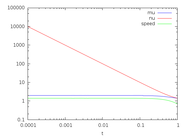
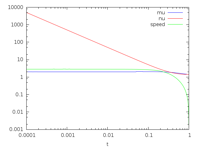
Figure 3. Logarithmic plot for the invariants associated to each of the solution paths, in the toric setting.

Running example, part 3.

Recall that $\mathbf{Z}^{(i)}(t)=(X^{(i)}(t),Y^{(i)}(t))$, $i=1,2$ are the two roots for $f_{t}$ in the running example (2). Let $\mathbf{z}^{(i)}(t)=\log\mathbf{Z}^{(i)}(t)$ coordinatewise, and let $g^{(i)}=g(\mathbf{z}^{(i)})$ be the metric matrix for $\langle\cdot,\cdot\rangle_{1,2}$.

In order to obtain an approximation for the integral $\mathscr{L}$, we first compute the Taylor series of the Hermitian matrix

$$\begin{split}M^{(i)}=2\|\mathbf{V}(\mathbf{z}^{(i)}(t)\|^{-2}\begin{pmatrix}\|f_{1}\|^{-1}&0\\ 0&\|f_{2}\|^{-1}\end{pmatrix}&(\mathbf{f}_{t}\cdot D\mathbf{V}(\mathbf{z}^{(i)}(t))\ g^{(i)}_{t}\\ &(\mathbf{f}_{t}\cdot D\mathbf{V}(\mathbf{z}^{(i)}(t))^{*}\ \begin{pmatrix}\|f_{1}\|^{-1}&0\\ 0&\|f_{2}\|^{-1}\end{pmatrix}.\end{split}$$

The factor of 2 comes from the fact that we use the product metric $\langle\cdot,\cdot\rangle=\langle\cdot,\cdot\rangle_{1}+\langle\cdot,\cdot\rangle_{2}$ in the definition of $\mu$ and $\|\dot{z}\|$. Then, $\mu^{(i)}=\sqrt{(}\|M^{-1}\|)$. The square of $\nu^{(i)}$ is the largest diagonal entry of the matrix

$$N^{(i)}=\left(A-\begin{pmatrix}1\\ 1\\ 1\\ 1\end{pmatrix}\mathbf{m}(\mathbf{z}^{(i)})\right)g^{(i)}\left(A-\begin{pmatrix}1\\ 1\\ 1\\ 1\end{pmatrix}\mathbf{m}(\mathbf{z}^{(i)})\right)^{T},$$

where $A=\begin{pmatrix}1&0\\ 0&2\\ 1&1\\ 0&3\end{pmatrix}$ encodes the support and $\mathbf{m}$ is the momentum map. Computations for $\mu^{(i)}$, $\nu^{(i)}$ and the speed vector are displayed in Table 2. Actual values of the invariants appear in Figure 3 We obtain in both cases that

$$\mathscr{L}((\mathbf{f}_{t},\mathbf{z}_{t}^{(i)});\epsilon,1)=\int_{\epsilon}^{1}\mu^{(i)}\nu^{(i)}\|\cdots\|\,\mathrm{d}t=2\log(\epsilon^{-1})+O(1).$$

$i$ $1$ $2$ $\|(f_{1})_{t}\|^{2}$ $(t^{2}+1)^{2}$ $(t^{2}+1)^{2}$ $\|(f_{2})_{t}\|^{2}$ 4 4 $\|\mathbf{V}(\mathbf{z}^{(i)}(t))\|_{i}^{2}$ $2t^{-6}+O(t^{-4})$ $\frac{1}{2}t^{-2}+O(1)$ $g^{(i)}(t)$ $\begin{pmatrix}\frac{1}{4}&-\frac{1}{2}\\ -\frac{1}{2}&1+t^{2}+O(t^{4})\end{pmatrix}$ $\begin{pmatrix}4t^{2}&-8t^{2}\\ -8t^{2}&\frac{1}{4}+16t^{2}\end{pmatrix}+O(t^{4})$ $f\cdot D\mathbf{V}(\mathbf{z}^{(i)})$ $\begin{pmatrix}-t^{-2}+t^{-1}&t^{-2}-3t^{-1}\\ t^{-3}+t^{-2}&-t^{-3}-t^{-2}\end{pmatrix}$ $\begin{pmatrix}-1-t^{2}&\frac{3}{2}+\frac{5}{2}t^{2}\\ 0&\frac{1}{2}t^{-1}+1+t/2\end{pmatrix}$ $M^{(i)}$ $\begin{pmatrix}\frac{1}{4}+\frac{1}{2}t&-\frac{1}{2}t\\ -\frac{1}{2}t&\frac{1}{4}+\frac{1}{2}t\end{pmatrix}+O(t^{2})$ $\begin{pmatrix}\frac{1}{4}&-\frac{1}{2}t\\ -\frac{1}{2}t&\frac{1}{4}+t\end{pmatrix}+O(t^{2})$ $(\mu^{i})^{2}$ $4+O(t)$ $4+O(t)$ $(\nu^{(i)})^{2}$ $t^{-2}+1$ $\frac{1}{4}t^{-2}+\frac{3}{2}+\frac{1}{4}t^{2}$ $\left\|\frac{\partial}{\partial t}\left(\mathbf{f}_{t},\mathbf{z}^{(i)}(t)\right)\right\|_{\left(\mathbf{f}_{t},\mathbf{z}^{(i)}(t)\right)}^{2}$ $1-2t^{2}+O(t^{4})$ $4-56t^{2}+O(t^{4})$ $\left(\mu^{(i)}\nu^{(i)}\left\|\frac{\partial}{\partial t}\left(\mathbf{f}_{t},\mathbf{z}^{(i)}(t)\right)\right\|_{\left(\mathbf{f}_{t},\mathbf{z}^{(i)}(t)\right)}\right)^{2}$ $4t^{-2}+O(t^{-1})$ $4t^{-2}+O(t^{-1})$ $\mu^{(i)}\nu^{(i)}\left\|\frac{\partial}{\partial t}\left(\mathbf{f}_{t},\mathbf{z}^{(i)}(t)\right)\right\|_{\left(\mathbf{f}_{t},\mathbf{z}^{(i)}(t)\right)}$ $2t^{-1}+O(1)$ $2t^{-1}+O(1)$ $\mathscr{L}((\mathbf{f}_{t},\mathbf{z}_{t}^{(i)});\epsilon,1)=\int_{\epsilon}^{1}\mu^{(i)}\nu^{(i)}\sqrt{\|\dot{\mathbf{f}}_{t}\|_{\mathbf{f}_{t}}^{2}+\|\dot{\mathbf{z}}_{t}\|_{\mathbf{z}_{t}}^{2}}\,\mathrm{d}t$ $2\log(\epsilon^{-1})+O(1)$ $2\log(\epsilon^{-1})+O(1)$

Table 2. Computation of the condition length in the toric setting.

4. Distortion bounds

Newton iteration is usually generalized to manifolds through the use of geodesics and of the exponential map. Given a function or a vector field $f$ defined on a manifold $M$, the Newton vector field at this point evaluates to $\mathbf{w}=-D\mathbf{f}({\mathbf{x}})^{-1}\mathbf{f}(\mathbf{x})\in T_{\mathbf{x}}M$. Then ${\mathbf{N}}_{\mathbf{f},\mathbf{x}}$ is usually defined to be $\exp_{\mathbf{x}}(\mathbf{w})$, where $\exp_{\mathbf{x}}(t\|\mathbf{w}\|^{-1}\mathbf{w})$ is the geodesic passing at $\mathbf{x}$ for $t=0$ with tangent vector $\mathbf{w}/\|\mathbf{w}\|$ and constant unit speed. This point can be found by solving the geodesic differential equation, or by integrating it. Dedieu-Priouret-Malajovich generalized Smale’s invariants to this context using high order covariant derivatives and parallel transport. A sharper analysis for equations defined by fiber bundles on a manifold was carried out by Li-Wang.

Unfortunately, computing geodesics can be as hard as solving systems of equations. Indeed, let $\mathbf{f}:M\rightarrow\mathbb{C}^{n}$ be a holomorpic map from an $n$-dimensional complex manifold onto $\mathbb{C}^{n}$, and assume that the Hermitian structure of $M$ is the pull-back by $\mathbf{f}$ of the canonical Hermitian structure. If $\mathbf{x}_{0}\in M$ is an arbitrary point and $\mathbf{y}_{0}=\mathbf{f}(\mathbf{x}_{0})$, then the segment $[\mathbf{y}_{0},0]\subset\mathbb{C}^{n}$ pulls back to a minimizing geodesic $\mathbf{x}(t)$ with $\dot{\mathbf{x}}(0)=-D\mathbf{f}(\mathbf{x}_{0})^{-1}\mathbf{y}_{0}$ and $\mathbf{f}(\mathbf{x}(1))=0$. Of course, one may be able to compute efficiently geodesics on the sphere, on projective space and many interesting manifolds. No easy formula seems to be known for geodesics on toric varieties.

In this paper we traded the geodesics for straight lines in a unique canonical chart. This is topologically equivalent outside toric infinity, and is geometrically equivalent up to order 1. The Newton operator is much easier to compute, and no covariant derivatives are needed. There is a price to pay for bypassing geodesics. Parallel transport is not available any more. Each point has a different Hermitian structure associated to it. In this section we bound the distortion introduced by this trivial transport operator. As usual, the momentum map is the key to bound this distortion.

4.1. The momentum map

Since the momentum map $\mathbf{m}_{i}(\mathbf{x})$ plays such an important rôle in the theory, we need to estimate how fast it changes with respect to $\mathbf{x}$. The theorem below shows that the momentum is locally Lipschitz, and allows to compute local Lipschitz constants.

Theorem 4.1.1.

Let $1\leq i\leq n$ be fixed. Let $\mathbf{x},\mathbf{y}\in\mathscr{M}$. If $\nu_{i}(\mathbf{x})\|\mathbf{y}-\mathbf{x}\|_{i,\mathbf{x}}\leq s$ then

1. For any $\mathbf{w}\in\mathbb{R}^{n}$, $|(\mathbf{m}_{i}(\mathbf{y})-\mathbf{m}_{i}(\mathbf{x}))\mathbf{w}|\leq\|\mathbf{w}\|_{i,\mathbf{x}}(e^{2s}-1)e^{e^{2s}-1-2s}$.

2. Let $d$ be the Riemannian distance in $(\mathscr{M},\|\cdot\|_{i,\mathbf{x}})$. Then $\|\mathbf{m}_{i}(\mathbf{y})-\mathbf{m}_{i}(\mathbf{x})\|_{2}\leq 2\,\mathrm{diam}(\mathrm{Conv}(A_{i}))\,d(\mathbf{y},\mathbf{x})$.

Before proving the statement, we should point out an immediate consequences of Theorem 4.1.1(b). A point $\mathbf{v}\in\mathscr{V}$ is said to be at toric infinity if it has no preimage in $\mathscr{M}$.

Corollary 4.1.2.

Let $\mathbf{x}\in\mathscr{M}$ and let $\delta$ be the minimum over all $i$ of the Euclidean distance from $\mathbf{m}_{i}(\mathbf{x})$ to $\partial\mathrm{Conv}(A_{i})$, divided by the diamater of $\mathrm{Conv}(A_{i})$. Then, the open ball $B([\mathbf{V}(\mathbf{x})],\delta/2)\subset\mathscr{V}$ contains no point at toric infinity.

By dividing the induced Fubini-Study volume form by the total volume of $\mathscr{V}$, one makes $\mathscr{V}$ into a probability space. The momentum map is volume preserving, up to a constant. Therefore,

Corollary 4.1.3.

The probability that $\mathbf{v}\in\mathscr{V}$ is at distance at most $\delta/2$ from a point at toric infinity is at most

$$\delta\sum_{i=1}^{n}\frac{\mathrm{diam}(\mathrm{Conv}(A_{i}))\mathrm{Vol}(\partial\mathrm{Conv}(A_{i}))}{\mathrm{Vol}(\mathrm{Conv}(A_{i}))}.$$

Proof of Theorem 4.1.1.

Assume without loss of generality that $\mathbf{m}_{i}(\mathbf{x})=0$. Since the momentum $\mathbf{m}_{i}(\mathbf{y})$ depends only on the real part of $\mathbf{y}$, assume also that $\mathbf{x}$ and $\mathbf{y}$ are real. For $k\geq 1$, define

$$S_{k}(\mathbf{y})=2^{k-1}\sum_{a\in A_{i}}\rho_{\mathbf{a}}^{2}e^{2\mathbf{a}\mathbf{y}}\underbrace{\mathbf{a}\otimes\cdots\otimes\mathbf{a}}_{\text{$k$ times}}.$$

The momentum map is given by the formula

$$\mathbf{m}_{i}(\mathbf{y})=-\frac{1}{2}\phi(\mathbf{y})S_{1}(\mathbf{y})$$

with $\phi(\mathbf{y})=-2/\|V_{i}\|^{2}=-2/\sum_{\mathbf{a}\in A_{i}}|\rho_{\mathbf{a}}e^{\mathbf{a}\mathbf{y}}|^{2}$. The derivation rules for $\phi$ and $S_{k}$ are:

$$D\phi(\mathbf{y}) = \phi(\mathbf{y})^{2}S_{1}(\mathbf{y})$$

$$DS_{k}(\mathbf{y}) = S_{k+1}(\mathbf{y})$$

The first derivatives of $\mathbf{m}(\mathbf{y})$ are

$$D\mathbf{m}_{i}(\mathbf{y}) = -\frac{1}{2}\left(\rule{0.0pt}{12.91663pt}\phi(x)S_{2}(\mathbf{y})+\phi(\mathbf{y})^{2}S_{1}(\mathbf{y})^{2}\right)$$

$$D^{2}\mathbf{m}_{i}(\mathbf{y}) = -\frac{1}{2}\mathrm{Avg}\left(\rule{0.0pt}{12.91663pt}\phi(\mathbf{y})S_{3}(\mathbf{y})+3\phi(\mathbf{y})^{2}S_{2}(\mathbf{y})S_{1}(\mathbf{y})+\phi(\mathbf{y})^{3}S_{1}(\mathbf{y})^{3}\right)$$

$$D^{3}\mathbf{m}_{i}(\mathbf{y}) = -\frac{1}{2}\mathrm{Avg}\left(\rule{0.0pt}{12.91663pt}\phi(\mathbf{y})S_{4}(\mathbf{y})+4\phi(\mathbf{y})^{2}S_{3}(\mathbf{y})S_{1}(\mathbf{y})+3\phi(\mathbf{y})^{3}S_{2}(\mathbf{y})S_{2}(\mathbf{y})\right.$$

$$\left.+6\phi(\mathbf{y})^{3}S_{2}(\mathbf{y})S_{1}(\mathbf{y})^{2}+\phi(\mathbf{y})^{4}S_{1}(\mathbf{y})^{4}\rule{0.0pt}{12.91663pt}\right)$$

where average is taken over all permutations acting on the arguments of the $j+1$-linear form within parentheses. Recall that $D^{j}m_{i}(\mathbf{y})=D^{j+1}\frac{1}{2}\log K(\mathbf{y},\mathbf{y})$ so it should be a symmetric tensor. The averaging above can be understood as a symmetrization operator. It is convenient to represent each term of the form $\mathrm{Avg}\left(\phi(\mathbf{y})^{k}S_{i_{1}}(\mathbf{y})\cdots S_{i_{k}}(\mathbf{y})\right)$ by the Young diagram for the partition $j+1=i_{1}+i_{2}+\cdots i_{k}$. For instance when $j=3$ we write

$$D^{3}\mathbf{m}_{i}(\mathbf{y})=-\frac{1}{2}\left(\ytableausetup{smalltableaux}\ydiagram{4}+4\ydiagram{3,1}+3\ydiagram{2,2}+6\ydiagram{2,1,1}+\ydiagram{1,1,1,1}\right).$$

The coefficients to each Young diagram are the number of ways to partition a set of $j+1$ labeled elements into the corresponding partition. Indeed, the ‘derivative’ of a Young diagram is obtained by adding one box into every possible row, for instance

$$D\left(\ydiagram{2,1,1}\right)=\ydiagram{3,1,1}+\ydiagram{2,2,1}+\ydiagram{2,1,2}+\ydiagram{2,1,1,1}=\ydiagram{3,1,1}+2\ydiagram{2,2,1}+\ydiagram{2,1,1,1}$$

Using this notation,

$$D^{j}\mathbf{m}_{i}(\mathbf{y})=-\frac{1}{2}\sum_{Y}c_{Y}Y$$

where the sum ranges over all Young diagrams with $j+1$ boxes. A coarse bound for the norm of $D^{j}\mathbf{m}(\mathbf{y})$ is $\|D^{j}\mathbf{m}(\mathbf{y})\|\leq\frac{1}{2}\varpi_{j+1}\max\|Y\|$, where $\varpi_{j+1}=\sum_{Y}c_{Y}$ is the number of partitions of a set with $j+1$ labelled elements, known as the $j+1$-th Bell number, see Sloane’s OEIS OEIS*BELL sequence and Knuth’s book Knuth.

However we are actually bounding $\|D^{j}\mathbf{m}(\mathbf{x})\|$ under the assumption that $\mathbf{m}(\mathbf{x})=0$. In particular, $S_{1}(\mathbf{x})=0$ and Young diagrams with at least one length one row should not be counted. The number $\varpi^{\prime}_{j}$ of Young diagrams with $j$ boxes and no row of length one is also known as the number of complete rhyming schemes [OEIS]*sequence A000296, [Knuth] and has exponential generating function $c(t)=e^{e^{t}-1-t}$. The first values for $\varpi^{\prime}_{j}$ are

$$\varpi^{\prime}_{0}=1\hskip 10.00002pt\varpi^{\prime}_{1}=0\hskip 10.00002pt\varpi^{\prime}_{2}=1\hskip 10.00002pt\varpi^{\prime}_{3}=1\hskip 10.00002pt\varpi^{\prime}_{4}=4\hskip 10.00002pt\varpi^{\prime}_{5}=11\hskip 10.00002pt\varpi^{\prime}_{6}=41\hskip 10.00002pt\varpi^{\prime}_{7}=162$$

By using the fact that

$$\langle\mathbf{w}_{1},\mathbf{w}_{2}\rangle_{i,\mathbf{x}}=\langle D[V_{i}](\mathbf{x})\mathbf{w}_{1},D[V_{i}](\mathbf{x})\mathbf{w}_{2}\rangle=\|V_{i}(\mathbf{x})\|^{-2}\sum_{\mathbf{a}}\rho_{\mathbf{a}}e^{2\mathbf{a}\mathbf{x}}(\mathbf{a}\mathbf{w}_{1})(\mathbf{a}\mathbf{w}_{2}),$$

each $S_{k}$ can be bounded as follows:

$$|S_{k}(\mathbf{x})(\mathbf{w}_{1},\mathbf{w}_{2},\mathbf{w}_{3},\dots,\mathbf{w}_{k})| = 2^{k-1}\left|\sum_{\mathbf{a}}\rho_{\mathbf{a}}^{2}e^{2\mathbf{a}\mathbf{x}}(\mathbf{a}\mathbf{w}_{1})(\mathbf{a}\mathbf{w}_{2})(\mathbf{a}\mathbf{w}_{3})\cdots(\mathbf{a}\mathbf{w}_{k})\right|$$

$$\leq 2^{k-1}\left|\sum_{\mathbf{a}}\rho_{\mathbf{a}}^{2}e^{2\mathbf{a}\mathbf{x}}(\mathbf{a}\mathbf{w}_{1})(\mathbf{a}\mathbf{w}_{2})\right|\ \max_{\mathbf{a}}|\mathbf{a}\mathbf{w}_{3}|\cdots|\mathbf{a}\mathbf{w}_{k}|$$

$$\leq 2^{k-1}\|V_{i}(\mathbf{x})\|^{2}\left|\langle\mathbf{w}_{1},\mathbf{w}_{2}\rangle_{i,\mathbf{x}}\right|\max_{\mathbf{a}}|\mathbf{a}\mathbf{w}_{3}|\cdots|\mathbf{a}\mathbf{w}_{k}|$$

$$\leq 2^{k-1}\|V_{i}(x)\|^{2}\|\mathbf{w}_{1}\|_{i,\mathbf{x}}\|\mathbf{w}_{2}\|_{i,\mathbf{x}}\max_{\mathbf{a}}|\mathbf{a}\mathbf{w}_{3}|\cdots|\mathbf{a}\mathbf{w}_{k}|$$

Hence,

(10) $$|S_{k}(\mathbf{w}_{1},\dots,\mathbf{w}_{k})||\phi(\mathbf{x})|\leq 2^{k}\|\mathbf{w}_{1}\|_{i,\mathbf{x}}\|\mathbf{w}_{2}\|_{i,\mathbf{x}}\left(\max_{\mathbf{a}\in A}|\mathbf{a}\mathbf{w}_{3}|\cdots|\mathbf{a}\mathbf{w}_{k}|\right)$$

If $Y$ is a Young diagram, let $r(Y)$ be its number of rows. Let $w$ be an arbitrary vector. Adding over all the Young diagrams with $j+1$ cases and no row of length one,

$$\begin{split}|D^{j}\mathbf{m}_{i}(\mathbf{x})(\mathbf{w},\mathbf{y}-\mathbf{x},&\dots,\mathbf{y}-\mathbf{x})|\leq\\ \leq&\ 2^{j}\|\mathbf{w}\|_{i,\mathbf{x}}\sum_{Y}\|\mathbf{y}-\mathbf{x}\|_{i,\mathbf{x}}^{2r(Y)-1}\left(\max_{\mathbf{a}\in A_{i}}|\mathbf{a}(\mathbf{y}-\mathbf{x})|\right)^{j+1-2r(Y)}\\ \leq&\ 2^{j}\varpi^{\prime}_{j+1}\|\mathbf{w}\|_{i,\mathbf{x}}\|\mathbf{y}-\mathbf{x}\|_{i,\mathbf{x}}\left(\max_{\mathbf{a}\in A_{i}}|\mathbf{a}(\mathbf{y}-\mathbf{x})|\right)^{j-1}\end{split}$$

where the last inequality uses that $\|\mathbf{y}-\mathbf{x}\|_{i,\mathbf{x}}\leq\max_{\mathbf{a}\in A_{i}}|\mathbf{a}(\mathbf{y}-\mathbf{x})|$. Recall that $\mathbf{m}_{i}(\mathbf{x})=0$. The Taylor series of $\mathbf{m}_{i}(\mathbf{y})\mathbf{w}$ around $\mathbf{x}$ is:

$$\mathbf{m}_{i}(\mathbf{y})(\mathbf{w})=D\mathbf{m}_{i}(\mathbf{x})(\mathbf{w},\mathbf{y}-\mathbf{x})+\sum_{j\geq 2}\frac{1}{j!}D^{j}\mathbf{m}_{i}(\mathbf{x})(\mathbf{w},(\mathbf{y}-\mathbf{x})^{j}).$$

Let $c(t)=e^{e^{t}-1-t}$ be the exponential generating function for the number of complete rhyming schemes $\varpi^{\prime}_{j}$. We can bound:

$$|\mathbf{m}_{i}(\mathbf{y})\mathbf{w}| \leq \|\mathbf{w}\|_{i,\mathbf{x}}\|\mathbf{y}-\mathbf{x}\|_{i,\mathbf{x}}\sum_{j\geq 1}\frac{2}{j!}\varpi^{\prime}_{j+1}\left(2s\right)^{j-1}$$

$$\leq \frac{\|\mathbf{w}\|_{i,\mathbf{x}}\|\mathbf{y}-\mathbf{x}\|_{i,\mathbf{x}}}{s}\sum_{j\geq 1}\frac{1}{j!}\varpi^{\prime}_{j+1}\left(2s\right)^{j}$$

$$\leq \frac{\|\mathbf{w}\|_{i,\mathbf{x}}\|\mathbf{y}-\mathbf{x}\|_{i,\mathbf{x}}}{s}(c^{\prime}(2s)-\varpi^{\prime}_{1})$$

$$\leq \|\mathbf{w}\|_{i,\mathbf{x}}c^{\prime}(2s)$$

because $\varpi^{\prime}_{1}=0$ and $\|\mathbf{y}-\mathbf{x}\|_{i,\mathbf{x}}\leq\nu_{i}(\mathbf{x})\|\mathbf{y}-\mathbf{x}\|_{i,\mathbf{x}}=s$. Explicitly, $c^{\prime}_{1}(t)=(e^{t}-1)e^{e^{t}-1-t}$ so item (a) follows:

$$|\mathbf{m}_{i}(\mathbf{y})\mathbf{w}|\leq\|\mathbf{w}\|_{\mathbf{x}}(e^{2s}-1)e^{e^{2s}-1-2s}$$

In order to prove item (b), we apply the bound (10) to the formula $D\mathbf{m}_{i}(\mathbf{y})=-\frac{1}{2}\phi(\mathbf{y})S_{2}(\mathbf{y})$. One obtains:

$$|D\mathbf{m}_{i}(\mathbf{y})(\mathbf{w}_{1},\mathbf{w}_{2})|\leq\|\mathbf{w}_{1}\|_{i,\mathbf{x}}\|\mathbf{w}_{2}\|_{i,\mathbf{x}}.$$

Let $\mathbf{x}(t)_{t\in[0,T]}$ be a minimizing geodesic with respect to $\|\cdot\|_{i,\mathbf{x}}$ with boundary $\mathbf{x}(0)=\mathbf{x}$ and $\mathbf{x}(T)=\mathbf{y}$. Then,

$$|(\mathbf{m}_{i}(\mathbf{y})-\mathbf{m}_{i}(\mathbf{x}))(\mathbf{w}_{2})| = \left|\int_{0}^{T}D\mathbf{m}_{i}(\mathbf{x}(t))(\dot{\mathbf{x}}(t),\mathbf{w}_{2})\right|\,\mathrm{d}t$$

$$\leq \int_{0}^{T}2\|\dot{\mathbf{x}}(t)\|_{i,\mathbf{x}(t)}\|w_{2}\|_{i,\mathbf{x}(t)}\,\mathrm{d}t$$

$$\leq 2\max(\|\mathbf{w}_{2}\|_{i,\mathbf{x}(t)})\int_{0}^{T}\|\dot{\mathbf{x}}(t)\|_{i,\mathbf{x}(t)}\,\mathrm{d}t$$

$$\leq 2\max(\|\mathbf{w}_{2}\|_{i,\mathbf{x}(t)})d_{i}(x,y)$$

$$\leq 2\|\mathbf{w}_{2}\|\mathrm{diam}(\mathrm{Conv}(A_{i}))d_{i}(\mathbf{x},\mathbf{y})$$

where the last bound follows from the inequality $\|u\|_{i,\mathbf{x}}\leq\|\mathbf{w}\|_{2}\mathrm{diam}(\mathrm{Conv}(A_{i}))$. ∎

4.2. The local norms and the circumscribed radii

Proof of Lemma 3.4.5.

Assume without loss of generality that $\mathbf{m}_{i}(\mathbf{x})=0$ for all $i$. Write $\|\mathbf{w}\|_{i,\mathbf{y}}=\|Dv_{i}(\mathbf{y})\mathbf{w}\|$ where $v_{i}(\mathbf{x})=V_{i}(\mathbf{x})/\|V_{i}(\mathbf{x})\|$. In that case,

$$Dv_{i}(\mathbf{y})\mathbf{w}=Dv_{i}(\mathbf{x})\mathbf{w}+\sum_{k\geq 2}\frac{1}{k-1!}D^{k}v_{i}(\mathbf{w},\mathbf{y}-\mathbf{x},\cdots\mathbf{y}-\mathbf{x}).$$

Also,

$$D^{k}v_{i}(\mathbf{x})(\mathbf{w},\mathbf{y}-\mathbf{x},\cdots,\mathbf{y}-\mathbf{x})=\frac{1}{\|V_{i}(\mathbf{x})\|}\begin{pmatrix}\vdots\\ \rho_{\mathbf{a}}e^{\mathbf{a}\mathbf{x}}(\mathbf{a}\mathbf{w})(\mathbf{a}(\mathbf{y}-\mathbf{x}))^{k-1}\\ \vdots\end{pmatrix}$$

so

$$\left\|D^{k}v_{i}(\mathbf{x})(\mathbf{w},\mathbf{y}-\mathbf{x},\cdots,\mathbf{y}-\mathbf{x})\right\| \leq \left\|\frac{1}{\|V_{i}(\mathbf{x})\|}\begin{pmatrix}\vdots\\ \rho_{\mathbf{a}}e^{\mathbf{a}\mathbf{x}}(\mathbf{a}\mathbf{w})\\ \vdots\end{pmatrix}\right\|\max_{\mathbf{a}\in A_{i}}|\mathbf{a}(\mathbf{y}-\mathbf{x})|^{k-1}$$

$$= \|D[V_{i}](\mathbf{x})\mathbf{w}\|\max_{\mathbf{a}\in A_{i}}|\mathbf{a}(\mathbf{y}-\mathbf{x})|^{k-1}$$

Therefore,

$$\|Dv_{i}(\mathbf{y})\mathbf{w}-Dv_{i}(\mathbf{x})\mathbf{w}\|\leq\|\mathbf{w}\|_{i,\mathbf{x}}\sum_{k\geq 2}\frac{(\max_{\mathbf{a}\in A_{i}}|\mathbf{a}(\mathbf{y}-\mathbf{x})|)^{k-1}}{k-1!}\leq\|\mathbf{w}\|_{i,\mathbf{x}}\left(e^{s}-1\right).$$

Triangular inequality yields

$$(2-e^{s})\|\mathbf{w}\|_{i,\mathbf{x}}\leq\|\mathbf{w}\|_{i,\mathbf{y}}\leq e^{s}\|\mathbf{w}\|_{i,\mathbf{x}}$$

so the first statement follows. The second statement is now obvious. ∎

The circumscribed radii $\nu_{i}$ were crucial in our previous bounds. For later use, we also estimate their variation rate.

Lemma 4.2.1.

Let $1\leq i\leq n$. Let $\mathbf{x}\in\mathscr{M}$ and $\nu_{i}(\mathbf{x})\|\mathbf{y}-\mathbf{x}\|_{i,\mathbf{x}}\leq s$. Then,

$$\left(\nu_{i}(\mathbf{x})-(e^{2s}-1)e^{e^{2s}-1-2s}\right)e^{-s}\leq\nu_{i}(\mathbf{y})\leq\left(\nu_{i}(\mathbf{x})+(e^{2s}-1)e^{e^{2s}-1-2s}\right)\frac{1}{2-e^{s}}.$$

It follows immediately that if $\nu(\mathbf{x})\|\mathbf{y}-\mathbf{x}\|_{\mathbf{x}}\leq s$,

$$\left(\nu(\mathbf{x})-(e^{2s}-1)e^{e^{2s}-1-2s}\right)e^{-s}\leq\nu(\mathbf{y})\leq\left(\nu(\mathbf{x})+(e^{2s}-1)e^{e^{2s}-1-2s}\right)\frac{1}{2-e^{s}}$$

as well.

Proof.

In the sequel we drop the $i$ index so $A=A_{i}$, $\nu=\nu_{i}$, $\|\cdot\|_{\mathbf{x}}=\|\cdot\|_{i,\mathbf{x}}$, etc… We introduce the notation $\nu_{\mathbf{x}}(\mathbf{y})=\max_{\|\mathbf{u}\|_{\mathbf{x}}=1}|(\mathbf{a}-\mathbf{m}(\mathbf{y}))\mathbf{u}|$ so $\nu_{\mathbf{x}}(\mathbf{x})=\nu(\mathbf{x})$. From triangular inequality,

$$\nu_{\mathbf{x}}(\mathbf{x})-\|\mathbf{m}(\mathbf{y})-\mathbf{m}(\mathbf{x})\|_{\mathbf{x}}\leq\nu_{\mathbf{x}}(\mathbf{y})\leq\nu_{\mathbf{x}}(\mathbf{x})+\|\mathbf{m}(\mathbf{y})-\mathbf{m}(\mathbf{x})\|_{\mathbf{x}}$$

so

(11) $$(\nu_{\mathbf{x}}(\mathbf{x})-\max\|\mathbf{m}(\mathbf{y})-\mathbf{m}(\mathbf{x})\|_{\mathbf{x}})\frac{\nu_{y}(\mathbf{y})}{\nu_{\mathbf{x}}(\mathbf{y})}\leq\nu(\mathbf{y})\leq(\nu_{\mathbf{x}}(\mathbf{x})+\max\|\mathbf{m}(\mathbf{y})-\mathbf{m}(\mathbf{x})\|_{\mathbf{x}})\frac{\nu_{y}(\mathbf{y})}{\nu_{\mathbf{x}}(\mathbf{y})}.$$

From Lemma 3.4.5, $(2-e^{s})\|{\mathbf{w}}\|_{\mathbf{x}}\leq\|{\mathbf{w}}\|_{y}\leq e^{s}\|{\mathbf{w}}\|_{\mathbf{x}}$ so

$$\nu_{\mathbf{y}}(\mathbf{y}) = \sup_{\|\mathbf{w}\|_{\mathbf{y}}\leq 1}\max_{\mathbf{a}\in A}|(\mathbf{a}-\mathbf{m}(\mathbf{y}))\mathbf{w}|$$

$$\leq \frac{1}{2-e^{s}}\sup_{\|\mathbf{w}\|_{\mathbf{x}}\leq 1}\max_{\mathbf{a}\in A}|(\mathbf{a}-\mathbf{m}(\mathbf{y}))\mathbf{w}|$$

$$= \frac{1}{2-e^{s}}\nu_{\mathbf{x}}(\mathbf{y})$$

and

$$\nu_{\mathbf{y}}(\mathbf{y}) = \sup_{\|\mathbf{w}\|_{\mathbf{y}}\leq 1}\max_{\mathbf{a}\in A}|(\mathbf{a}-\mathbf{m}(\mathbf{y}))\mathbf{w}|$$

$$\geq \frac{1}{e^{s}}\sup_{\|\mathbf{w}\|_{\mathbf{x}}\leq 1}\max_{\mathbf{a}\in A}|(\mathbf{a}-\mathbf{m}(\mathbf{y}))\mathbf{w}|$$

$$= \frac{1}{e^{s}}\nu_{\mathbf{x}}(\mathbf{y})$$

The last two bounds and Theorem 4.1.1(a) can be substituted into equation (11):

$$\left(\nu(\mathbf{x})-(e^{2s}-1)e^{e^{2s}-1-2s}\right)e^{-s}\leq\nu(\mathbf{y})\leq\left(\nu(\mathbf{x})+(e^{2s}-1)e^{e^{2s}-1-2s}\right)\frac{1}{2-e^{s}}$$

∎

4.3. The condition number

Toward the proof of Theorem 3.4.6, we will show the following estimate. It should be compared to Burgisser-Cucker*Prop. 16.55. The extra factor $1+O(s)$ comes from the different local norms.

Theorem 4.3.1.

Let $[\mathbf{f}],[\mathbf{g}]\in\mathbb{P}(\mathscr{F}_{1}),\dots,\mathbb{P}(\mathscr{F}_{n})$. Let $\mathbf{x}\in\mathscr{M}$. Assume that for all $i$, $\nu_{i}(\mathbf{x})\|\mathbf{y}-\mathbf{x}\|_{i,\mathbf{x}}\leq s$. If $\mu(\mathbf{f},\mathbf{x})\left(d_{P}(\mathbf{f},\mathbf{g})+(e^{s}-1)\right)<1$, then

$$\frac{\left(2-e^{s}\right)\mu(\mathbf{f},\mathbf{x})}{1+\mu(\mathbf{f},\mathbf{x})\left(d_{P}(\mathbf{f},\mathbf{g})+(e^{s}-1)\right)}\leq\mu(\mathbf{g},\mathbf{y})\leq\frac{e^{s}\mu(\mathbf{f},\mathbf{x})}{1-\mu(\mathbf{f},\mathbf{x})\left(d_{P}(\mathbf{f},\mathbf{g})+(e^{s}-1)\right)}$$

where $d_{P}$ is the multiprojective (sine) distance.

In the proof of Theorem 4.3.1 we will need two well-known Lemmas about linear mappings between normed spaces. The proofs are included for completeness.

Lemma 4.3.2.

Let $A$ and $B$ be linear operators between finite dimensional normed spaces. Let $\sigma(X)=\inf_{\|\mathbf{u}\|\leq 1}\|Xu\|$ and let $\|X\|$ denote the operator norm of $X$. Then,

$$|\sigma(A)-\sigma(B)|\leq\|A-B\|$$

Proof.

Assume that $\sigma(A)=\|A\mathbf{u}\|$ with $\|\mathbf{u}\|=1$. Triangular inequality yields

$$\sigma(A)=\|A\mathbf{u}\|\geq\|B\mathbf{u}\|-\|(A-B)\mathbf{u}\|\geq\sigma(B)-\|A-B\|.$$

Replacing $A$ by $B$ one obtains that $\sigma(B)\geq\sigma(A)-\|A-B\|$. ∎

Lemma 4.3.3.

Let $A,B$ be invertible linear operators between finite dimensional normed spaces. If $\|A^{-1}\|\|A-B\|<1$, then

$$\frac{\|A^{-1}\|}{1+\|A^{-1}\|\|A-B\|}\leq\|B^{-1}\|\leq\frac{\|A^{-1}\|}{1-\|A^{-1}\|\|A-B\|}$$

Proof.

From the previous Lemma,

$$\frac{1}{\|A^{-1}\|}-\|A-B\|\leq\frac{1}{\|B^{-1}\|}\leq\frac{1}{\|A^{-1}\|}+\|A+B\|.$$

Multiplying by $\|A^{-1}\|\|B^{-1}\|$,

$$\|B^{-1}\|(1-\|A^{-1}\|\|A-B\|)\leq\|A^{-1}\|\leq\|B^{-1}\|(1+\|A^{-1}\|\|A-B\|)$$

and so

$$\frac{\|A^{-1}\|}{1+\|A^{-1}\|\|A-B\|}\leq\|B^{-1}\|\leq\frac{\|A^{-1}\|}{1-\|A^{-1}\|\|A-B\|}$$

∎

Proof of Theorem 4.3.1.

Assume without loss of generality that $\mathbf{m}_{i}(\mathbf{x})=0$ for all $i$. Also without loss of generality, scale the $f_{i}$ such that $\|f_{1}\|=\cdots=\|f_{n}\|=1$ and the $g_{i}$ such that $\|f_{i}-g_{i}\|$ is minimal, so $d_{P}(\mathbf{f},\mathbf{g})=\|\mathbf{f}-\mathbf{g}\|$. Let $v_{i}(\mathbf{x})=\frac{1}{\|V_{i}(\mathbf{x})\|}V_{i}(\mathbf{x})$. Because $\mathbf{m}_{i}(\mathbf{x})=0$ for all $i$, we can write

$$\mu(\mathbf{f},\mathbf{x})=\left\|(\mathbf{f}\cdot Dv(\mathbf{x}))^{-1}\right\|_{\mathbf{x}}$$

where $\mathbf{f}\cdot D\mathbf{v}(\mathbf{x})$ is an operator from $(\mathscr{M},\|\cdot\|_{\mathbf{x}})$ into $\mathbb{C}^{n}$ with the canonical norm assumed.

From the previous Lemma,

$$\frac{\mu(\mathbf{f},\mathbf{x})}{1+\mu(\mathbf{f},\mathbf{x})T}\leq\left\|(\mathbf{g}\cdot D\mathbf{v}(\mathbf{y}))^{-1}\right\|_{\mathbf{x}}\leq\frac{\mu(\mathbf{f},\mathbf{x})}{1-\mu(\mathbf{f},\mathbf{x})T}$$

where $T=\left\|\mathbf{f}\cdot D\mathbf{v}(\mathbf{x})-\mathbf{g}\cdot D\mathbf{v}(\mathbf{y})\right\|_{\mathbf{x}}$. We estimate $T=T^{\prime}+T^{\prime\prime}$ where

$$T^{\prime} = \left\|\mathbf{f}\cdot D\mathbf{v}(\mathbf{x})-\mathbf{g}\cdot D\mathbf{v}(\mathbf{x})\right\|_{\mathbf{x}}$$

$$\leq \sup_{\|\mathbf{w}\|_{\mathbf{x}}\leq 1}\left\|(\mathbf{f}-\mathbf{g})\cdot D\mathbf{v}(\mathbf{x})\mathbf{w}\right\|$$

$$\leq \sup_{\|\mathbf{w}\|_{\mathbf{x}}\leq 1}\sqrt{\sum\|f_{i}-g_{i}\|^{2}}\max_{i}\|\mathbf{w}\|_{i,\mathbf{x}}$$

$$\leq \|\mathbf{f}-\mathbf{g}\|$$

and

$$T^{\prime\prime} = \left\|\mathbf{g}\cdot D\mathbf{v}(\mathbf{x})-\mathbf{g}\cdot D\mathbf{v}(\mathbf{y})\right\|_{\mathbf{x}}$$

$$= \sup_{\|\mathbf{w}\|_{\mathbf{x}}\leq 1}\sqrt{\sum_{i}|g_{i}(Dv_{i}(\mathbf{x})-Dv_{i}(\mathbf{y}))\mathbf{w}|^{2}}$$

$$\leq \sup_{\|\mathbf{w}\|_{\mathbf{x}}\leq 1}\sqrt{\sum_{i}\|g_{i}\|^{2}}\max_{i}\|(Dv_{i}(\mathbf{x})-Dv_{i}(\mathbf{y}))\mathbf{w}\|$$

$$\leq \sup_{\|\mathbf{w}\|_{\mathbf{x}}\leq 1}\max_{i}\|(Dv_{i}(\mathbf{x})-Dv_{i}(\mathbf{y}))\mathbf{w}\|$$

$$\leq \max_{i}\sup_{\|\mathbf{w}\|_{i,\mathbf{x}}\leq 1}\sum_{k\geq 2}\frac{1}{k-1!}\|D^{k}v_{i}(\mathbf{x})(\mathbf{w},\mathbf{y}-\mathbf{x},\cdots,\mathbf{y}-\mathbf{x})\|$$

$$\leq \max_{i}\sum_{k\geq 2}\frac{1}{k-1!}\nu_{i}(\mathbf{x})^{k-1}\|\mathbf{y}-\mathbf{x}\|_{i,\mathbf{x}}^{k-1}$$

$$\leq (e^{s}-1)$$

Therefore,

$$\frac{\left(2-e^{s}\right)\mu(\mathbf{f},\mathbf{x})}{1+\mu(\mathbf{f},\mathbf{x})\left(\|\mathbf{f}-\mathbf{g}\|+(e^{s}-1)\right)}\leq\mu(\mathbf{g},\mathbf{y})\leq\frac{e^{s}\mu(\mathbf{f},\mathbf{x})}{1-\mu(\mathbf{f},\mathbf{x})\left(\|\mathbf{f}-\mathbf{g}\|+(e^{s}-1)\right)}$$

∎

We are ready to prove Theorem 3.4.6.

Proof of Theorem 3.4.6.

Let $s=\max_{i}\nu_{i}(\mathbf{x})\|\mathbf{y}-\mathbf{x}\|_{i,\mathbf{x}}$ and recall that $\mu(\mathbf{f},\mathbf{x})\nu(\mathbf{x})$ $(\|\mathbf{y}-\mathbf{x}\|_{\mathbf{x}}+d_{P}(\mathbf{f},\mathbf{g}))\leq\theta$. The right-hand sides of Lemma 4.2.1 can be bounded above by

$$\nu(\mathbf{y}) \leq \left(\nu(\mathbf{x})+(e^{2s}-1)e^{e^{2s}-1-2s}\right)\frac{1}{2-e^{s}}$$

$$\leq \nu(\mathbf{x})\left(1+(e^{2\theta}-1)e^{e^{2\theta}-1-2\theta}\right)\frac{1}{2-e^{\theta}}$$

using $\nu(\mathbf{x})\geq 1$ and $s=\nu(\mathbf{x})\|\mathbf{x}-\mathbf{y}\|_{\mathbf{x}}\leq\theta$. The right hand side of Theorem  4.3.1 satisfies

$$\mu(\mathbf{g},\mathbf{y}) \leq \frac{e^{s}\mu(\mathbf{f},\mathbf{x})}{1-\mu(\mathbf{f},\mathbf{x})\left(d_{P}(\mathbf{f}-\mathbf{g})+(e^{s}-1)\right)}$$

$$\leq \frac{e^{s}\mu(\mathbf{f},\mathbf{x})}{2-e^{\theta}}$$

using $\mu(\mathbf{f},\mathbf{x})(e^{s}-1)\leq e^{\mu(\mathbf{f},\mathbf{x})\nu(\mathbf{x})\|\mathbf{x}-\mathbf{y}\|_{\mathbf{x}}}-1$ and hence $\mu(\mathbf{f},\mathbf{x})\left(d_{P}(\mathbf{f}-\mathbf{g})+(e^{s}-1)\right)$ $\leq e^{\theta}-1$. Putting all together,

$$\mu(\mathbf{g},\mathbf{y})\nu(\mathbf{y})\leq\mu(\mathbf{f},\mathbf{x})\nu(\mathbf{x})e^{u}\frac{1+(e^{2\theta}-1)e^{e^{2\theta}-1-2\theta}}{\left(2-e^{\theta}\right)^{2}}\leq\frac{\mu(\mathbf{f},\mathbf{x})\nu(\mathbf{x})}{1-5\theta}.$$

By a similar argument,

$$\mu(\mathbf{g},\mathbf{y})\nu(\mathbf{y})\geq\mu(\mathbf{f},\mathbf{x})\nu(\mathbf{x})\frac{(1-(e^{2\theta}-1)e^{e^{2\theta}-1-2\theta})(2-e^{\theta})}{e^{2\theta}}\geq(1-5\theta)\mu(\mathbf{f},\mathbf{x})\nu(\mathbf{x}).$$

∎

5. Proof of the technical results

5.1. Proof of the toric $\gamma$-theorem

For the proof of Theorem 3.5.1 we will need the following fact, which can be stated as a general result about the $\gamma$ invariant. Let $\kappa(X)=\|X\|\|X^{-1}\|$ be the Wilkinson condition number for a square matrix $X$, where operator norms are assumed:

Lemma 5.1.1.

Let $\mathbf{z}\in\mathbb{C}^{n}$ be fixed, and let $\mathbf{f}:U\rightarrow\mathbb{C}^{n}$ with $\mathbf{f}(\mathbf{z})=0$ be holomorphic on a neighborhood of $\mathbf{z}$. Let $\mathbf{m}_{1},\dots,\mathbf{m}_{n}\in(\mathbb{C}^{n})^{*}$ and set $g_{i}(\mathbf{x})=e^{-m_{i}\cdot\mathbf{x}}f_{i}(\mathbf{x})$. If $\mathbf{f}(\mathbf{z})=0$ then

$$\gamma(\mathbf{g},\mathbf{z})\leq\kappa(D\mathbf{f}(\mathbf{z}))\max_{i}\sup_{\|\mathbf{w}\|_{{\mathbf{z}}}\leq 1}|\mathbf{m}_{i}(\mathbf{w})|+\gamma(\mathbf{f},\mathbf{z}).$$

Proof of Lemma 5.1.1.

We differentiate $g_{i}$ to obtain

$$Dg_{i}(\mathbf{x})=e^{-\mathbf{m}_{i}\cdot\mathbf{x}}\left(Df_{i}(\mathbf{x})-f_{i}(\mathbf{x})\mathbf{m}_{i}\right).$$

Since $\mathbf{g}$ vanishes at $\mathbf{z}$, we have $Dg_{i}(\mathbf{z})=e^{-\mathbf{m}_{i}\cdot\mathbf{z}}Df_{i}(\mathbf{z})$. By induction,

$$D^{k}g_{i}(\mathbf{x})=e^{-\mathbf{m}_{i}\cdot\mathbf{x}}\sum_{l=0}^{k}(-1)^{l}\left(\begin{matrix}k\\ l\end{matrix}\right)\mathrm{Avg}\left(D^{k-l}f_{i}(\mathbf{x})\otimes\mathbf{m}_{i}^{\otimes l}\right)$$

where the average is taken over all the permutations of the covariant indices. In order to bound $\gamma(\mathbf{g},\mathbf{z})$, we will produce a bound for $\frac{\|D\mathbf{g}(\mathbf{z})^{-1}D^{k}\mathbf{g}(\mathbf{z})\|_{\mathbf{z}}}{k!}$. For clarity, we examine first the case $k=2$. Assume that the operator norm of $\frac{1}{2}D\mathbf{g}(\mathbf{z})^{-1}D^{2}\mathbf{g}(\mathbf{z})$ is attained at unit vectors $\mathbf{w}_{1}$ and $\mathbf{w}_{2}$, that is

$$\left\|\frac{1}{2}D\mathbf{g}(\mathbf{z})^{-1}D^{2}\mathbf{g}(\mathbf{z})\right\|_{{\mathbf{z}}}=\left\|\frac{1}{2}D\mathbf{g}(\mathbf{z})^{-1}D^{2}\mathbf{g}(\mathbf{z})(\mathbf{w}_{1},\mathbf{w}_{2})\right\|_{{\mathbf{z}}}$$

where $\|\mathbf{w}_{1}\|_{{\mathbf{z}}}=\|\mathbf{w}_{2}\|_{{\mathbf{z}}}=1$. Expand

$$\frac{1}{2}D\mathbf{g}(\mathbf{z})^{-1}D^{2}\mathbf{g}(\mathbf{z})(\mathbf{w}_{1},\mathbf{w}_{2}) = \frac{1}{2}D\mathbf{f}(\mathbf{z})^{-1}D^{2}\mathbf{f}(\mathbf{z})(\mathbf{w}_{1},\mathbf{w}_{2})$$

$$- \frac{1}{2}D\mathbf{f}(\mathbf{z})^{-1}\left[\begin{matrix}\mathbf{m}_{1}\cdot\mathbf{w}_{1}\\ &\ddots\\ &&\mathbf{m}_{n}\cdot\mathbf{w}_{1}\end{matrix}\right]D\mathbf{f}(\mathbf{z})\mathbf{w}_{2}$$

$$- \frac{1}{2}D\mathbf{f}(\mathbf{z})^{-1}\left[\begin{matrix}\mathbf{m}_{1}\cdot\mathbf{w}_{2}\\ &\ddots\\ &&\mathbf{m}_{n}\cdot\mathbf{w}_{2}\end{matrix}\right]D\mathbf{f}(\mathbf{z})\mathbf{w}_{1}.$$

Taking norms, $\|\frac{1}{2}D\mathbf{g}(\mathbf{z})^{-1}D^{2}\mathbf{g}(\mathbf{z})(\mathbf{w}_{1},\mathbf{w}_{2})\|_{{\mathbf{z}}}\leq\gamma(\mathbf{f},\mathbf{z})+\kappa(D\mathbf{f}(\mathbf{z}))\max_{i}\|\mathbf{m}_{i}\|_{{\mathbf{z}}}$. The general case is similar. Assume that the operator norm of $\frac{1}{k!}D\mathbf{g}(\mathbf{z})^{-1}D^{k}\mathbf{g}(\mathbf{z})$ is attained at $\mathbf{w}_{1},\dots,\mathbf{w}_{k}$, namely

$$\left\|\frac{1}{k!}D\mathbf{g}(\mathbf{z})^{-1}D^{k}\mathbf{g}(\mathbf{z})\right\|_{{\mathbf{z}}}=\left\|\frac{1}{k!}D\mathbf{g}(\mathbf{z})^{-1}D^{k}\mathbf{g}(\mathbf{z})(\mathbf{w}_{1},\dots,\mathbf{w}_{k})\right\|_{{\mathbf{z}}}$$

with $\|\mathbf{w}_{1}\|_{{\mathbf{z}}}=\cdots=\|\mathbf{w}_{k}\|_{{\mathbf{z}}}$. Then,

$$\begin{split}\frac{1}{k!}D\mathbf{g}(\mathbf{z})^{-1}D^{k}\mathbf{g}(\mathbf{z})(\mathbf{w}_{1},\dots,\mathbf{w}_{k})&=\\ =\frac{1}{k!}\sum_{l=0}^{k-1}(-1)^{l}\left(\begin{matrix}k\\ l\end{matrix}\right)\mathrm{Avg}&\left(D\mathbf{f}(\mathbf{z})^{-1}M(\mathbf{w}_{1},\dots,\mathbf{w}_{l})D^{k-l}\mathbf{f}(\mathbf{z})(\mathbf{w}_{l+1},\dots,\mathbf{w}_{k})\right)\end{split}$$

with

$$M(\mathbf{w}_{1},\dots,\mathbf{w}_{l})\stackrel{{\scriptstyle\mathrm{def}}}{{=}}\left[\begin{matrix}\prod_{j=1}^{l}\mathbf{m}_{1}\cdot\mathbf{w}_{j}\\ &\ddots\\ &&\prod_{j=1}^{l}\mathbf{m}_{n}\cdot\mathbf{w}_{j}\end{matrix}\right].$$

Taking norms,

$$\frac{1}{k!}\left\|D\mathbf{g}(\mathbf{z})^{-1}D^{k}\mathbf{g}(\mathbf{z})\right\|_{{\mathbf{z}}} \leq \frac{1}{k!}\sum_{l=0}^{k-1}\left(\begin{matrix}k\\ l\end{matrix}\right)\mathrm{Avg}\left\|D\mathbf{f}(\mathbf{z})^{-1}M(\mathbf{w}_{1},\dots,\mathbf{w}_{l})\right.$$

$$\hskip 90.00015pt\left.D^{k-l}\mathbf{f}(\mathbf{z})(\mathbf{w}_{l+1},\dots,\mathbf{w}_{k})\right\|_{{\mathbf{z}}}$$

$$\leq \frac{1}{k!}\sum_{l=0}^{k-1}\left(\begin{matrix}k\\ l\end{matrix}\right)\mathrm{Avg}\left\|D\mathbf{f}(\mathbf{z})^{-1}M(\mathbf{w}_{1},\dots,\mathbf{w}_{l})D\mathbf{f}(\mathbf{z})\right\|_{{\mathbf{z}}}$$

$$\hskip 90.00015pt\left\|D\mathbf{f}(\mathbf{z})^{-1}D^{k-l}\mathbf{f}(\mathbf{z})(\mathbf{w}_{l+1},\dots,\mathbf{w}_{k})\right\|_{{\mathbf{z}}}$$

When $l=0$ we have $\left\|D\mathbf{f}(\mathbf{z})^{-1}M(\mathbf{w}_{1},\dots,\mathbf{w}_{l})D\mathbf{f}(\mathbf{z})\right\|_{{\mathbf{z}}}=1$. Otherwise, its value can be bounded above by $\kappa(D\mathbf{f}(\mathbf{z}))\max_{i,j}(|\mathbf{m}_{i}\cdot\mathbf{w}_{j}|)^{l}$. Using the fact that $\kappa(D\mathbf{f}(\mathbf{z}))\geq 1$, we bound

$$\frac{1}{k!}\left\|D\mathbf{g}(\mathbf{z})^{-1}D^{k}\mathbf{g}(\mathbf{z})\right\|_{{\mathbf{z}}} \leq \sum_{l=0}^{k-1}\frac{1}{l!}\kappa(D\mathbf{f}(\mathbf{z}))\max_{i,j}(|\mathbf{m}_{i}\cdot\mathbf{w}_{j}|)^{l}\frac{\left\|D\mathbf{f}(\mathbf{z})^{-1}D^{k-l}\mathbf{f}(\mathbf{z})\right\|_{{\mathbf{z}}}}{k-l!}$$

$$\leq \sum_{l=0}^{k-1}\left(\begin{matrix}k-1\\ l\end{matrix}\right)\kappa(D\mathbf{f}(\mathbf{z}))^{l}(\max_{ij}|\mathbf{m}_{i}\cdot\mathbf{w}_{j}|)^{l}\gamma(\mathbf{f},\mathbf{z})^{k-l-1}$$

$$\leq \left(\kappa(D\mathbf{f}(\mathbf{z}))\max_{ij}|\mathbf{m}_{i}\cdot\mathbf{w}_{j}|+\gamma(\mathbf{f},\mathbf{z})\right)^{k-1}$$

Taking $k-1$-th roots, we obtain:

$$\gamma(\mathbf{g},\mathbf{z})\leq\kappa(D\mathbf{f}(\mathbf{x}))\max_{ij}|\mathbf{m}_{i}\cdot\mathbf{w}_{j}|+\gamma(\mathbf{f},\mathbf{z}).$$

∎

We will need the following, well-known Lemma. Since the proof is short, it is included for completeness.

Lemma 5.1.2.

Let $\mathbf{g}:(\mathbb{E},\|\cdot\|)\rightarrow(\mathbb{F},\|\cdot\|)$ be a holomorphic map between Banach spaces. Let ${u}=\|\mathbf{z}-\mathbf{x}\|\gamma(\mathbf{g},\mathbf{z})<1-\frac{\sqrt{2}}{2}$. Then, $D\mathbf{g}(\mathbf{x})$ is invertible and

(12) $$\|D\mathbf{g}(\mathbf{x})^{-1}D\mathbf{g}(\mathbf{z})\|\leq\frac{(1-u^{2})}{\psi(u)}$$

where $\psi(u)=1-4u+2u^{2}$.

Proof.

$$\|(D\mathbf{g}(\mathbf{z}))^{-1}D\mathbf{g}(\mathbf{x})-I\| \leq \sum_{k\geq 2}\frac{\left\|(D\mathbf{g}(\mathbf{z}))^{-1}D^{k}\mathbf{g}(\mathbf{z})\right\|}{k-1!}{\|\mathbf{x}-\mathbf{z}\|}^{k-1}$$

$$\leq \sum_{k\geq 2}k\gamma(\mathbf{g},\mathbf{z})^{k-1}\|\mathbf{x}-\mathbf{z}\|^{k-1}$$

$$= \frac{1}{(1-u)^{2}}-1.$$

Therefore $D\mathbf{g}(\mathbf{z}))^{-1}D\mathbf{g}(\mathbf{x})$ is invertible and

$$\|D\mathbf{g}(\mathbf{x})^{-1}D\mathbf{g}(\mathbf{z})\|\leq\frac{1}{1-\left(\frac{1}{(1-u)^{2}}-1\right)}=\frac{(1-u^{2})}{\psi(u)}$$

and equation (12) holds. ∎

Proof of Theorem 3.5.1.

We assume without loss of generality that $\mathbf{m}_{i}(\mathbf{z})=0$. For each $i$, we use the $i$-th momentum map to produce an ‘integrating factor’ at $\mathbf{x}_{0}$: Set $W_{i}(\mathbf{x})=e^{-\mathbf{m}_{i}(\mathbf{x}_{0})({\mathbf{x}})}V_{i}(\mathbf{x})$. Then

$$f_{i}\cdot\frac{1}{\|V_{i}(\mathbf{x}_{0})\|}P_{V_{i}^{\perp}}DV_{i}(\mathbf{x}_{0}) = f_{i}\cdot\frac{1}{\|V_{i}(\mathbf{x}_{0})\|}\left(I-\frac{1}{\|V_{i}(\mathbf{x}_{0})\|^{2}}V_{i}(\mathbf{x}_{0})V_{i}(\mathbf{x}_{0})^{*}\right)DV_{i}(\mathbf{x}_{0})$$

$$= f_{i}\cdot\frac{1}{\|V_{i}(\mathbf{x}_{0})\|}DV_{i}(\mathbf{x}_{0})-f_{i}\cdot\frac{1}{\|V_{i}(\mathbf{x}_{0})\|}V_{i}(\mathbf{x}_{0})\mathbf{m}_{i}(\mathbf{x}_{0})$$

$$= e^{{\mathbf{m}_{i}}(\mathbf{x}_{0})\mathbf{x}_{0}}f_{i}\cdot\frac{1}{\|V_{i}(\mathbf{x}_{0})\|}DW_{i}(\mathbf{x}_{0})$$

$$= f_{i}\cdot\frac{1}{\|W_{i}(\mathbf{x}_{0})\|}DW_{i}(\mathbf{x}_{0})$$

The toric Newton operator takes $\mathbf{x}_{0}$ to $\mathbf{x}_{1}={\mathbf{N}}_{\mathbf{f}}(\mathbf{x}_{0})$ where

$$\mathbf{x}_{1} = \mathbf{x}_{0}-\left({\mathbf{f}}\cdot(I-P_{V(\mathbf{x}_{0})^{\perp}})D\mathbf{V}(\mathbf{x}_{0})\right)^{-1}\mathbf{f}\cdot\mathbf{V}(\mathbf{x}_{0})$$

$$= \mathbf{x}_{0}-(\mathbf{f}\cdot D\mathbf{W}(\mathbf{x}_{0}))^{-1}\mathbf{f}\cdot\mathbf{W}(\mathbf{x}_{0})$$

Thus, the toric Newton operator at $\mathbf{x}_{0}$ is the same as the usual Newton operator at $\mathbf{x}_{0}$ for the function $\mathbf{g}(\mathbf{x})=\mathbf{f}\cdot\|\mathbf{W}(\mathbf{x}_{0})\|^{-1}\mathbf{W}(\mathbf{x})$. This differs from the local section by a ratio

$$\mathbf{g}(\mathbf{x})=S_{\mathbf{f},\mathbf{x}_{0}}(\mathbf{x}-\mathbf{z})e^{-\mathbf{m}_{i}(\mathbf{x}_{0})\mathbf{x}}$$

Also, $\mathbf{g}(\mathbf{z})=0$.

From now on we use the metric structure of $T_{\mathbf{z}}\mathscr{M}$. All norms, operator norms and the invariant $\gamma$ are computed with the norm $\|\cdot\|_{\mathbf{z}}$. Lemma 5.1.1 provides the bound

$$\gamma(\mathbf{g},\mathbf{z})=\kappa(DS_{\mathbf{f},\mathbf{z}}(0))\max_{i}\|\mathbf{m}_{i}(\mathbf{x}_{0})\|_{\mathbf{z}}+\gamma(\mathbf{f},\mathbf{z})$$

where $\kappa(DS_{\mathbf{f},\mathbf{z}}(0))=\|DS_{\mathbf{f},\mathbf{z}}(0)\|_{\mathbf{z}}\|DS_{\mathbf{f},\mathbf{z}}(0)^{-1}\|_{\mathbf{z}}\leq\mu(\mathbf{f},\mathbf{x})$ using operator norms. Above, $\|\mathbf{m}_{i}(\mathbf{x}_{0})\|_{\mathbf{z}}=\max_{\|\mathbf{w}\|_{\mathbf{z}}\leq 1}|\mathbf{m}_{i}(\mathbf{x}_{0})\mathbf{w}|$ is the norm of $\mathbf{m}_{i}(\mathbf{x}_{0})$ as a covector. Since we took $\mathbf{m}_{i}(\mathbf{z})=0$, $\|\mathbf{m}_{i}(\mathbf{x}_{0})\|_{\mathbf{z}}=\|\mathbf{m}_{i}(\mathbf{x}_{0})-\mathbf{m}_{i}(\mathbf{z})\|_{\mathbf{z}}$. Therefore,

$$\|\mathbf{x}_{0}-\mathbf{z}\|_{\mathbf{z}}\gamma(\mathbf{g},\mathbf{z})\leq\gamma(\mathbf{f},\mathbf{z})+\mu(\mathbf{f},\mathbf{z})\|\|\mathbf{m}_{i}(\mathbf{x}_{0})-\mathbf{m}_{i}(\mathbf{z})\|_{\mathbf{z}}\leq\frac{3-\sqrt{7}}{2}.$$

By Theorem 2.1.1 applied to $\mathbf{g}$ one would achieve quadratic convergence yet for a different Newton operator, namely $\mathbf{x}\mapsto\mathbf{x}-(\mathbf{f}\cdot P_{\mathbf{V}(\mathbf{x}_{0})^{\perp}}D\mathbf{V}(\mathbf{x}))^{-1}\cdot\mathbf{V}(\mathbf{x})$. Instead, we just claim that for $\mathbf{x}_{1}={\mathbf{N}}_{\mathbf{f}}(\mathbf{x}_{0})$,

(13) $$\|\mathbf{x}_{1}-\mathbf{z}\|_{\mathbf{z}}\leq\|\mathbf{x}_{0}-\mathbf{z}\|_{\mathbf{z}}\frac{u}{\psi(u)}$$

where $\mathbf{u}=\gamma(\mathbf{g},\mathbf{z})\|\mathbf{x}_{0}-\mathbf{z}\|_{\mathbf{z}}$ and $\psi(u)=1-4u+2u^{2}$. If we define the sequence $u_{i}=\gamma(\mathbf{g},\mathbf{z})\|\mathbf{x}_{i}-\mathbf{z}\|_{\mathbf{z}}$, we deduce from (13) that

$$u_{i+1}\leq\frac{u_{i}^{2}}{\psi(u)}.$$

This is enough to deduce that the $u_{i}$ decrease faster than the iterates of $t_{0}=0$, $t_{i+1}={\mathbf{N}}_{h_{\gamma}}(t_{i})$, for $h_{\gamma}(t)=t-\frac{\gamma t^{2}}{1-\gamma t}$, $\gamma=\gamma(\mathbf{f},\mathbf{z})$. This in turn implies that

$$u_{i}\leq 2^{-2^{i}+1}u_{0}$$

and hence

$$\|\mathbf{x}_{i}-\mathbf{z}\|_{\mathbf{z}}\leq 2^{-2^{i}+1}\|\mathbf{x}_{0}-\mathbf{z}\|_{\mathbf{z}}.$$

It remains to prove (13). Set $W_{i}(\mathbf{x})=e^{-\mathbf{m}_{i}(\mathbf{x}_{0})(\mathbf{x})}V_{i}(\mathbf{x})$. As before, $u=\gamma(\mathbf{g},\mathbf{z})\|\mathbf{x}_{0}-\mathbf{z}\|$. Then

$$\mathbf{x}_{1}-\mathbf{z} = \mathbf{x}_{0}-\mathbf{z}-\left(\mathbf{f}\cdot(I-P_{\mathbf{V}(\mathbf{x}_{0})^{\perp}})D\mathbf{V}(\mathbf{x}_{0})\right)^{-1}\mathbf{f}\cdot\mathbf{V}(\mathbf{x}_{0})$$

$$= \mathbf{x}_{0}-\mathbf{z}-D\mathbf{g}(\mathbf{x}_{0}))^{-1}\mathbf{g}(\mathbf{x}_{0})$$

$$= (D\mathbf{g}(\mathbf{x}_{0}))^{-1}\left(D\mathbf{g}(\mathbf{x}_{0})(\mathbf{x}_{0}-\mathbf{z})-\mathbf{g}(\mathbf{x}_{0})\right)$$

$$= (D\mathbf{g}(\mathbf{x}_{0}))^{-1}(D\mathbf{g}(\mathbf{z}))(D\mathbf{g}(\mathbf{z}))^{-1}\left(D\mathbf{g}(\mathbf{x}_{0})(\mathbf{x}_{0}-\mathbf{z})-\mathbf{g}(\mathbf{x}_{0})\right)$$

For all vector $\mathbf{w}$, we can expand

$$D\mathbf{g}(\mathbf{x}_{0})\mathbf{w}=D\mathbf{g}(\mathbf{z})\mathbf{w}+\sum_{k\geq 2}\frac{1}{k-1!}D^{k}\mathbf{g}(\mathbf{z})((\mathbf{x}_{0}-\mathbf{z})^{k-1},\mathbf{w}).$$

Lemma 5.1.2 applied to $\mathbf{g}:(T_{\mathbf{z}}\mathscr{M},\|\cdot\|_{\mathbf{z}})\rightarrow(\mathbb{C}^{n},\|\cdot\|_{2})$ implies that

$$\|D\mathbf{g}(\mathbf{x}_{0})^{-1}D\mathbf{g}(\mathbf{z})\|_{\mathbf{z}}\leq\frac{(1-u)^{2}}{\psi(u)}$$

with $\psi(u)=1-4u+2u^{2}$. It remains to bound

$$(D\mathbf{g}(\mathbf{z}))^{-1}\left(D\mathbf{g}(\mathbf{x}_{0})(\mathbf{x}_{0}-\mathbf{z})-\mathbf{g}(\mathbf{x}_{0})\right)=\sum_{k\geq 2}\frac{k-1}{k!}(D\mathbf{g}(\mathbf{z}))^{-1}D^{k}\mathbf{g}(\mathbf{z})(\mathbf{x}_{0}-\mathbf{z})^{k}$$

by

$$\left\|(D\mathbf{g}(\mathbf{z}))^{-1}(\cdots)\right\|_{\mathbf{z}}\leq\sum_{k\geq 2}(k-1)u^{k-1}\|\mathbf{x}_{0}-\mathbf{z}\|_{\mathbf{z}}=\frac{u\|\mathbf{x}_{0}-\mathbf{z}\|_{{\mathbf{z}}}}{(1-u)^{2}}.$$

This shows that $\|\mathbf{x}_{1}-\mathbf{z}\|_{\mathbf{z}}\leq\|\mathbf{x}_{0}-\mathbf{z}\|_{\mathbf{z}}\frac{u}{\psi(u)}$, establishing (13).

∎

5.2. The higher derivative estimate

Proof of Theorem 3.6.1.

Assume without loss of generality that $\mathbf{m}_{i}(\mathbf{x})=0$ for all $i$.

$$\frac{1}{k!}\left\|DS_{\mathbf{f},\mathbf{x}}(0)^{-1}D^{k}S_{\mathbf{f},\mathbf{x}}(0)\right\|_{\mathbf{x}}\leq$$

$$\leq \frac{1}{k!}\left\|DS_{\mathbf{f},\mathbf{x}}(0)^{-1}\begin{pmatrix}\|f_{1}\|\\ &\ddots\\ &&\|f_{n}\|\end{pmatrix}\right\|_{\mathbf{x}}\left\|\begin{pmatrix}\frac{1}{\|f_{1}\|}f_{1}\cdot\frac{1}{\|V_{1}(\mathbf{x})\|}D^{k}V_{1}(\mathbf{x})\\ \vdots\\ \frac{1}{\|f_{n}\|}f_{n}\cdot\frac{1}{\|V_{n}(\mathbf{x})\|}D^{k}V_{n}(\mathbf{x})\end{pmatrix}\right\|_{\mathbf{x}}$$

$$\leq \frac{1}{k!}\mu(\mathbf{f},\mathbf{x})\left\|\begin{pmatrix}\frac{1}{\|V_{1}(\mathbf{x})\|}D^{k}V_{1}(\mathbf{x})\\ \vdots\\ \frac{1}{\|V_{n}(\mathbf{x})\|}D^{k}V_{n}(\mathbf{x})\end{pmatrix}\right\|_{\mathbf{x}}$$

$$\leq \frac{1}{k!}\mu(\mathbf{f},\mathbf{x})\nu(\mathbf{x})^{k-1}$$

as in the proof of Lemma 3.4.5. Then use the fact that $\mu(\mathbf{f},\mathbf{x})\geq 1$ to bound the expression above by

$$\frac{1}{k!}\left\|DS_{\mathbf{f},\mathbf{x}}(0)^{-1}D^{k}S_{\mathbf{f},\mathbf{x}}(0)\right\|_{\mathbf{x}}\leq\frac{1}{2^{k-1}}\mu(\mathbf{f},\mathbf{x})^{k-1}\nu(\mathbf{x})^{k-1},$$

before taking $k-1$-th roots. ∎

5.3. Proof of the modified gamma theorem

Proof of Theorem 3.6.2.

Assume that $u=\frac{1}{2}\|\mathbf{x}_{0}-\mathbf{z}\|_{\mathbf{z}}\mu(\mathbf{f},\mathbf{z})\nu(\mathbf{z})\leq\frac{3-\sqrt{7}}{2}$. From Theorem 3.6.1 we can bound

$$\|\mathbf{x}_{0}-\mathbf{z}\|_{\mathbf{z}}\gamma(\mathbf{f},\mathbf{z})\leq u$$

From Theorem  4.1.1(a) and bounding $s\leq 2u$,

$$\|\mathbf{x}_{0}-\mathbf{z}\|_{\mathbf{z}}\mu(\mathbf{f},\mathbf{z})\max_{i}\sup_{\|\mathbf{w}\|_{\mathbf{z}}=1}|(\mathbf{m}_{i}(\mathbf{z})-\mathbf{m}_{i}(\mathbf{x}))\mathbf{w}|\leq 2u(e^{4u}-1)e^{e^{4u}-1-4u}.$$

The inequality $u+2u(e^{4u}-1)e^{e^{4u}-1-4u}\leq\frac{3-\sqrt{7}}{2}$ holds for $u\leq u_{0}=0.090994609\cdots$, where $u_{0}$ was obtained numerically. ∎

5.4. Proof of Proposition 3.7.1

Proof.

Since $\mathbf{f}(\mathbf{z})=0$,

$$D\mathbf{f}(\mathbf{z})^{-1}\mathbf{f}(\mathbf{x})=\mathbf{x}-\mathbf{z}+\sum_{k\geq 2}\frac{1}{k!}D\mathbf{f}(\mathbf{z})^{-1}D^{k}\mathbf{f}(\mathbf{z})(\mathbf{x}-\mathbf{z})^{k}$$

so that

$$\|D\mathbf{f}(\mathbf{z})^{-1}\mathbf{f}(\mathbf{x})\|_{\mathbf{z}} \leq \|\mathbf{x}-\mathbf{z}\|_{\mathbf{z}}\left(1+\sum_{k\geq 2}\gamma(\mathbf{f},\mathbf{z})^{k-1}\|\mathbf{x}-\mathbf{z}\|_{\mathbf{z}}^{k-1}\right)$$

$$= \frac{\|\mathbf{x}-\mathbf{z}\|_{\mathbf{z}}}{1-\gamma(\mathbf{f},\mathbf{z})\|\mathbf{x}-\mathbf{z}\|_{\mathbf{z}}}$$

Since $\|\mathbf{x}-\mathbf{z}\|_{\mathbf{z}}\gamma(\mathbf{f},\mathbf{z})\|\leq u\leq 1/10<1-\sqrt{2}/2$, Lemma 5.1.2 allows us to bound

$$\|D\mathbf{f}(\mathbf{x})^{-1}\mathbf{f}(\mathbf{x})\|_{\mathbf{z}} \leq \|D\mathbf{f}(\mathbf{x})^{-1}D\mathbf{f}(\mathbf{z})\|_{\mathbf{z}}\|D\mathbf{f}(\mathbf{z})^{-1}\mathbf{f}(\mathbf{x})\|_{\mathbf{z}}$$

$$\leq \frac{(1-u)^{2}}{\psi(u)}\frac{\|\mathbf{x}-\mathbf{z}\|_{\mathbf{z}}}{1-\gamma(\mathbf{f},\mathbf{z})\|\mathbf{x}-\mathbf{z}\|_{\mathbf{z}}}$$

with $\psi(u)=1-4u+2u^{2}$. Theorem 3.6.1 and Lemma 3.4.5 with $s\leq 2u$ imply

$$\beta(\mathbf{f},\mathbf{x})=\|D\mathbf{f}(\mathbf{x})^{-1}\mathbf{f}(\mathbf{x})\|_{\mathbf{x}}\leq e^{2u}\frac{1-u}{\psi(u)}\|\mathbf{x}-\mathbf{z}\|_{\mathbf{z}}$$

Also, Theorem 3.4.6 with $\theta\leq 2u$ implies that

$$\mu(\mathbf{f},\mathbf{x})\nu(\mathbf{x})\leq\frac{\mu(\mathbf{z})\nu(\mathbf{z})}{1-10u}$$

so

$$\frac{1}{2}\mu(\mathbf{f},\mathbf{x})\nu(\mathbf{x})\beta(\mathbf{f},\mathbf{x})\leq ue^{2u}\frac{1-u}{\psi(u)(1-10u)}$$

∎

6. Finsler structure

The toric variety associated to an unmixed system of sparse polynomial equations has $n$ natural Hermitian metrics, each one induced by the support of one of the equations. In Section 3.3 we added up all those Hermitian metrics to produce one Hermitian metric, namely

$$\langle\cdot,\cdot\rangle_{\mathbf{x}}=\langle\cdot,\cdot\rangle_{1,\mathbf{x}}+\cdots+\langle\cdot,\cdot\rangle_{n,\mathbf{x}}.$$

This metric cannot be a natural object. Each of the $n$ Hermitian metrics is actually induced by a Kahler symplectic form, and the mixed volume is the integral over the toric variety of the wedge product of those $n$ forms, up to a constant. By adding the Hermitian metrics, information is lost. Instead, a formal linear combination

$$\lambda_{1}\langle\cdot,\cdot\rangle_{1,\mathbf{x}}+\cdots+\lambda_{n}\langle\cdot,\cdot\rangle_{n,\mathbf{x}}$$

would preserve the mixed volume information, the mixed volume being proportional to the coefficient in $\lambda_{1}\cdots\lambda_{n}$ of the total volume. Those linear combinations are induced by a semigroup structure on the space of spaces of fewnomials, see [Malajovich-Fewspaces] and the discussion therein.

Therefore, it may be more natural to measure lengths on $\mathscr{V}$ and $\mathscr{M}$ in some way that is invariant of the coefficients $\lambda_{1},\dots,\lambda_{n}>0$. Instead of using the Hermitian norm

$$\|\cdot\|_{\mathbf{x}}=\sqrt{\langle\cdot,\cdot\rangle_{\mathbf{x}}}.$$

we can also use

$$\left\vvvert\mathbf{w}\right\vvvert_{\mathbf{x}}=\max_{i}\|\mathbf{w}\|_{i,\mathbf{x}}=\max_{i}\sqrt{\langle\mathbf{w},\mathbf{w}\rangle_{i,\mathbf{x}}}.$$

This associates a norm to each $\mathbf{x}$. Because each $\|\cdot\|_{i,\mathbf{x}}$ is rescaling invariant, $\left\vvvert\cdot\right\vvvert_{\mathbf{x}}$ is independent of the $\lambda_{i}$. We always have $\left\vvvert\mathbf{w}\right\vvvert_{\mathbf{x}}\leq\|\mathbf{w}\|_{\mathbf{x}}$. In the running example, $\left\vvvert\mathbf{w}\right\vvvert_{\mathbf{x}}=\frac{\sqrt{2}}{2}\|\mathbf{w}\|_{\mathbf{x}}$.

Remark 6.0.1.

Most authors define a Finsler structure as a function $F:T\mathcal{M}\rightarrow\mathbb{R}$ so that $F(\mathbf{x},\cdot)$ is a norm and $F(\mathbf{x},\dot{\mathbf{x}})$ is smooth or $\mathcal{C}^{1}$ for $\dot{\mathbf{x}}\neq 0$. The norm $\left\vvvert\mathbf{x}\right\vvvert_{\dot{\mathbf{x}}}$ is only guaranteed to be continuous and subdifferentiable. Properly speaking, one might call it a subdifferentiable Finsler structure.

Smale’s alpha-theory was originally stated for holomorphic mappings between Banach spaces. The definition of invariants $\beta$, $\gamma$ and $\alpha$ for a Newton operator $\mathbb{B}\rightarrow\mathbb{B}$ only uses the norm on $\mathbb{B}$ and the induced operator norm for multilinear maps. In the context of this paper, the invariants become

$$\beta(\mathbf{f},\mathbf{x})=\left\vvvert{\mathbf{N}}_{\mathbf{f}}(\mathbf{x})-\mathbf{x}\right\vvvert_{\mathbf{x}}=\left\vvvert DS_{\mathbf{f},\mathbf{x}}(0)^{-1}S_{\mathbf{f},\mathbf{x}}(0)\right\vvvert_{\mathbf{x}},$$

$$\gamma(\mathbf{f},\mathbf{x})\stackrel{{\scriptstyle\mathrm{def}}}{{=}}\max_{k\geq 2}\left(\frac{1}{k!}\sup_{\left\vvvert\mathbf{w}_{1}\right\vvvert_{\mathbf{x}},\dots,\left\vvvert\mathbf{w}_{k}\right\vvvert_{\mathbf{x}}\leq 1}\left\vvvert DS_{\mathbf{f},\mathbf{x}}(0)^{-1}D^{k}S_{\mathbf{f},\mathbf{x}}(0)(\mathbf{w}_{1},\dots,\mathbf{w}_{k})\right\vvvert_{\mathbf{x}}\right)^{\frac{1}{k-1}}$$

and $\alpha(\mathbf{f},\mathbf{x})=\beta(\mathbf{f},\mathbf{x})\gamma(\mathbf{f},\mathbf{x})$.

The invariant $\mu$ is more delicate. It was defined as the operator norm of the map

$$DG(f):\left(T_{[f_{1}]}\mathbb{P}(\mathscr{F}_{1})\times\cdots\times T_{[f_{n}]}\mathbb{P}(\mathscr{F}_{n}),\|\cdot\|_{\mathbf{x}}\right)\rightarrow(T_{\mathbf{x}}\mathscr{M},\|\cdot\|_{\mathbf{x}})$$

where the product norm was assumed in the domain of $DG(\mathbf{f})$. We redefine $\mu$ as the operator norm of the same map between different spaces. In the manifold

$$\mathbb{P}(\mathscr{F}_{1})\times\cdots\times\mathbb{P}(\mathscr{F}_{n})$$

we also define a Finsler structure,

$$\left\vvvert\dot{\mathbf{f}}\right\vvvert_{[\mathbf{f}]}=\max_{i}\|\dot{\mathbf{f}}_{i}\|_{[f_{i}]}.$$

Now,

$$DG(f):\left(T_{f_{1}}\mathbb{P}(\mathscr{F}_{1})\times\cdots\times T_{f_{n}}\mathbb{P}(\mathscr{F}_{n}),\left\vvvert\cdot\right\vvvert_{x}\right)\rightarrow(T_{\mathbf{x}}\mathscr{M},\left\vvvert\cdots\right\vvvert_{\mathbf{x}})$$

and the norm on the domain is

$$\left\vvvert\dot{\mathbf{f}}\right\vvvert_{[\mathbf{f}]}=\max_{i}\|\dot{\mathbf{f}}_{i}\|_{[f_{i}]}.$$

An alternative formulation is

$$\begin{split}\mu(\mathbf{f},\mathbf{x})&=\left\vvvert DS_{\mathbf{f},\mathbf{x}}(0)^{-1}\begin{pmatrix}\|f_{1}\|\\ &\ddots\\ &&\|f_{n}\|\end{pmatrix}\right\vvvert_{\infty,\mathbf{x}}\\ &=\left(\inf_{\left\vvvert\mathbf{w}\right\vvvert_{i,\mathbf{x}}\leq 1}\max_{i}\frac{|f_{i}\cdot DV_{i}(\mathbf{x})\mathbf{w}|}{\|\mathbf{f}\|_{i}}{\|V_{i}(\mathbf{x})\|}\right)^{-1}.\end{split}$$

The expression above guarantees that $\mu(\mathbf{f},\mathbf{x})\geq 1$ always. The invariant $\nu$ is already defined in terms of the $\|\cdot\|_{i,\mathbf{x}}$ so it does not change.

In the proof of Theorem 4.1.1, only the inner products $\langle\cdot,\cdot\rangle_{i,\mathbf{x}}$ appear, and this is the only place in the proof of Main Theorems A and B where an Hermitian structure is used.

The definition of the multiprojective metric in Theorem 3.4.6 should be modified to be compatible with the Finsler structure. Now,

$$d_{P}(\mathbf{f},\mathbf{g})=\max_{i}\inf_{\lambda\in\mathbb{C}}\frac{\|f_{i}-\lambda g_{i}\|}{\|f_{i}\|}.$$

As usual, $d_{P}(\mathbf{f},\mathbf{g})\leq d(\mathbf{f},\mathbf{g})$ where $d$ is the Finslerian distance from $\mathbf{f}$ to $\mathbf{g}$.

The proofs of Theorem 4.3.1 and 3.6.1 must be modified because of the operator norm $\left\vvvert\cdot\right\vvvert_{\infty,\mathbf{x}}$.

Proof of Theorem 4.3.1 for the Finsler structure.

We assume without loss of generality that $\mathbf{m}_{i}(\mathbf{x})=0$ for all $i$, scale the $f_{i}$ such that $\|f\|_{1}=\cdots=\|f_{n}\|=1$ and then scale the $g_{i}$ such that $\|f_{i}-g_{i}\|$ is minimal. The sine distance now is the sine distance for the Finsler metric, that is $d_{P}(\mathbf{f},\mathbf{g})=\max_{i}\|f_{i}-g_{i}\|$. Let $v_{i}(\mathbf{x})=\frac{1}{\|V_{i}(\mathbf{x})\|}V_{i}(\mathbf{x})$. Because $\mathbf{m}_{i}(\mathbf{x})=0$ for all $i$, we can write

$$\mu(\mathbf{f},\mathbf{x})=\left\vvvert(\mathbf{f}\cdot D\mathbf{v}(\mathbf{x}))^{-1}\right\vvvert_{\infty,\mathbf{x}}.$$

Lemma  4.3.3 provides us with the inequality

$$\frac{\mu(\mathbf{f},\mathbf{x})}{1+\mu(\mathbf{f},\mathbf{x})T}\leq\left\|(\mathbf{g}\cdot D\mathbf{v}(\mathbf{y}))^{-1}\right\|_{\mathbf{x}}\leq\frac{\mu(\mathbf{f},\mathbf{x})}{1-\mu(\mathbf{f},\mathbf{x})T}$$

where now, $T=\left\vvvert\mathbf{f}\cdot D\mathbf{v}(\mathbf{x})-\mathbf{g}\cdot D\mathbf{v}(\mathbf{y})\right\vvvert_{\mathbf{x},\infty}$. We estimate $T=T^{\prime}+T^{\prime\prime}$ where

$$T^{\prime} = \left\vvvert\mathbf{f}\cdot Dv(\mathbf{x})-\mathbf{g}\cdot D\mathbf{v}(\mathbf{x})\right\vvvert_{\mathbf{x},\infty}$$

$$\leq \sup_{\left\vvvert\mathbf{w}\right\vvvert_{\mathbf{x}}\leq 1}\max_{i}\left|(f_{i}-g_{i})\cdot Dv_{i}(\mathbf{x})\mathbf{w}\right\|$$

$$\leq \max_{i}\|f_{i}-g_{i}\|$$

and

$$T^{\prime\prime} = \left\vvvert\mathbf{g}\cdot D\mathbf{v}(\mathbf{x})-\mathbf{g}\cdot D\mathbf{v}(\mathbf{y})\right\vvvert_{\mathbf{x},\infty}$$

$$= \sup_{\left\vvvert\mathbf{w}\right\vvvert_{\mathbf{x}}\leq 1}\max_{i}\left|g_{i}(Dv_{i}(\mathbf{x})-Dv_{i}(\mathbf{y}))\mathbf{w}\right|$$

$$\leq \sup_{\left\vvvert\mathbf{w}\right\vvvert_{\mathbf{x}}\leq 1}\max_{i}\|(Dv_{i}(\mathbf{x})-Dv_{i}(\mathbf{y}))\mathbf{w}\|$$

$$\leq \sup_{\left\vvvert\mathbf{w}\right\vvvert_{\mathbf{x}}\leq 1}\max_{i}\sum_{k\geq 2}\frac{1}{k-1!}\|D^{k}v_{i}(\mathbf{x})(\mathbf{w},\mathbf{y}-\mathbf{x},\cdots,\mathbf{y}-\mathbf{x})\|$$

$$\leq \max_{i}\sum_{k\geq 2}\frac{1}{k-1!}\nu_{i}(\mathbf{x})^{k-1}\|\mathbf{y}-\mathbf{x}\|_{i,\mathbf{x}}^{k-1}$$

$$\leq (e^{s}-1)$$

As before,

$$\frac{\left(2-e^{s}\right)\mu(f,x)}{1+\mu(\mathbf{f},\mathbf{x})\left(\|\mathbf{f}-\mathbf{g}\|+(e^{s}-1)\right)}\leq\mu(\mathbf{g},\mathbf{y})\leq\frac{e^{s}\mu(\mathbf{f},\mathbf{x})}{1-\mu(\mathbf{f},\mathbf{x})\left(\|\mathbf{f}-\mathbf{g}\|+(e^{s}-1)\right)}$$

∎

Proof of Theorem 3.6.1 for the Finsler structure.

As before, assume without loss of generality that $\mathbf{m}_{i}(\mathbf{x})=0$ for all $i$.

$$\frac{1}{k!}\left\vvvert DS_{\mathbf{f},\mathbf{x}}(0)^{-1}D^{k}S_{\mathbf{f},\mathbf{x}}(0)\right\vvvert_{\mathbf{x}}\leq$$

$$\leq \frac{1}{k!}\left\vvvert DS_{\mathbf{f},\mathbf{x}}(0)^{-1}\begin{pmatrix}\|f_{1}\|\\ &\ddots\\ &&\|f_{n}\|\end{pmatrix}\right\vvvert_{\infty,\mathbf{x}}\left\vvvert\begin{pmatrix}\frac{1}{\|f_{1}\|}f_{1}\cdot\frac{1}{\|V_{1}(\mathbf{x})\|}D^{k}V_{1}(\mathbf{x})\\ \vdots\\ \frac{1}{\|f_{n}\|}f_{n}\cdot\frac{1}{\|V_{n}(\mathbf{x})\|}D^{k}V_{n}(\mathbf{x})\end{pmatrix}\right\vvvert_{\mathbf{x},\infty}$$

$$\leq \frac{1}{k!}\mu(\mathbf{f},\mathbf{x})\max_{i}\sup_{\left\vvvert\mathbf{w}_{1}\right\vvvert_{\mathbf{x}},\dots,\left\vvvert\mathbf{w}_{k}\right\vvvert_{\mathbf{x}}\leq 1}\left|\frac{1}{\|V_{i}(\mathbf{x})\|}D^{k}V_{i}(\mathbf{x})(\mathbf{w}_{1},\dots,\mathbf{w}_{k})\right|$$

$$\leq \frac{1}{k!}\mu(\mathbf{f},\mathbf{x})\nu(\mathbf{x})^{k-1}.$$

as in the proof of Lemma 3.4.5. We can still use $\mu(\mathbf{f},\mathbf{x})\geq 1$ to bound the expression above by

$$\frac{1}{k!}\left\vvvert DS_{\mathbf{f},\mathbf{x}}(0)^{-1}D^{k}S_{\mathbf{f},\mathbf{x}}(0)\right\vvvert_{\mathbf{x}}\leq\frac{1}{2^{k-1}}\mu(\mathbf{f},\mathbf{x})^{k-1}\nu(\mathbf{x})^{k-1},$$

and take $k-1$-th roots. ∎

7. Conclusions and future work

The theory of condition numbers and homotopy for sparse systems proposed in this paper shares many of the features of the theory of homotopy algorithms for dense polynomial systems: there are effective criteria for quadratic convergence, a Lipschitz condition number, a higher derivative estimate and the toric condition length is an upper bound for the cost of homotopy algorithms.

This bound is possibly sharper from what we would obtain from the theory of dense homogeneous or multi-homogeneous equations, as illustrated by the running example. On the other hand, this theory has some distinctive features.

The higher derivative estimate for $\gamma(\mathbf{f},\mathbf{x})$ is less sharp as $x$ goes to toric infinity. This is to be expected, since in the toric case ‘infinity’ means a supporting facet of the support. Therefore it may be necessary to ‘switch charts’ at some point and appromiate roots going to infinity by points at infinity. In the mean time, we are left with the undesirable features of the non-homogenized, later discarded version of the theory in Bezout1.

Nothing was said about implementation issues. Some of them may require experimentation. For instance, it is not clear if the extra sharpness provided by the Finsler structure does offset the extra cost of computing it. This may depend on how many variables appear on each polynomial.

Then we need a probabilistic analysis of the condition of sparse polynomial systems. This may be a challenging problem. Previous results obtained by  Malajovich-Rojas depend on polynomial systems being unmixed or on a mixed dilation which is only finite for nondegenerate fewnomial spaces as in Definition 3.1.1(iii). This is an inconvenient hypothesis. Removing it is a topic for future research.

AllgowerEugene L.GeorgKurtContinuation and path followingtitle={Acta numerica, 1993}, series={Acta Numer.}, publisher={Cambridge Univ. Press}, place={Cambridge}, 19931–64Review @article{AllgowerGeorg, author = {Allgower, Eugene L.}, author = {Georg, Kurt}, title = {Continuation and path following}, conference = {title={Acta numerica, 1993}, }, book = {series={Acta Numer.}, publisher={Cambridge Univ. Press}, place={Cambridge}, }, date = {1993}, pages = {1–64}, review = {\MR{1224680 (94k:65076)}}} ArmentanoDiegoBeltránCarlosBürgisserPeterCuckerFelipeShubMichaelCondition length and complexity for the solution of polynomial systemsFound. Comput. Math.201616 number=6 pages=1401–1422 issn=0272-4979Document@article{ABBCS, author = {Armentano, Diego}, author = {Beltrán, Carlos}, author = {Bürgisser, Peter}, author = {Cucker, Felipe}, author = {Shub, Michael}, title = {Condition Length and Complexity for the Solution of Polynomial Systems}, journal = {Found. Comput. Math.}, date = {2016}, volume = {{16} number={6} pages={1401–1422} issn={0272-4979}}, doi = {10.1007/s10208-016-9309-9}} BeltránCarlosA continuation method to solve polynomial systems and its complexityNumer. Math.1172011189–113ISSN 0029-599XReview Document@article{Beltran2011, author = {Beltr{\'a}n, Carlos}, title = {A continuation method to solve polynomial systems and its complexity}, journal = {Numer. Math.}, volume = {117}, date = {2011}, number = {1}, pages = {89–113}, issn = {0029-599X}, review = {\MR{2754220}}, doi = {10.1007/s00211-010-0334-3}} BeltránCarlosDedieuJean-PierreMalajovichGregorioShubMikeConvexity properties of the condition numberSIAM J. Matrix Anal. Appl.31200931491–1506ISSN 0895-4798Review Document@article{BDMS1, author = {Beltr{\'a}n, Carlos}, author = {Dedieu, Jean-Pierre}, author = {Malajovich, Gregorio}, author = {Shub, Mike}, title = {Convexity properties of the condition number}, journal = {SIAM J. Matrix Anal. Appl.}, volume = {31}, date = {2009}, number = {3}, pages = {1491–1506}, issn = {0895-4798}, review = {\MR{2587788}}, doi = {10.1137/080718681}} BeltránCarlosDedieuJean-PierreMalajovichGregorioShubMikeConvexity properties of the condition number iiSIAM J. Matrix Anal. Appl.3320123905–939ISSN 0895-4798Review Document@article{BDMS2, author = {Beltr{\'a}n, Carlos}, author = {Dedieu, Jean-Pierre}, author = {Malajovich, Gregorio}, author = {Shub, Mike}, title = {Convexity properties of the condition number II}, journal = {SIAM J. Matrix Anal. Appl.}, volume = {33}, date = {2012}, number = {3}, pages = {905–939}, issn = {0895-4798}, review = {\MR{3023457}}, doi = {10.1137/100808885}} BeltránCarlosLeykinAntonRobust certified numerical homotopy trackingFound. Comput. Math.1320132253–295ISSN 1615-3375Review Document@article{Beltran-Leykin, author = {Beltr{\'a}n, Carlos}, author = {Leykin, Anton}, title = {Robust certified numerical homotopy tracking}, journal = {Found. Comput. Math.}, volume = {13}, date = {2013}, number = {2}, pages = {253–295}, issn = {1615-3375}, review = {\MR{3032682}}, doi = {10.1007/s10208-013-9143-2}} BeltránCarlosPardoLuis MiguelSmale’s 17th problem: average polynomial time to compute affine and projective solutionsJ. Amer. Math. Soc.2220092363–385ISSN 0894-0347Review Document@article{Beltran-Pardo-2009, author = {Beltr{\'a}n, Carlos}, author = {Pardo, Luis Miguel}, title = {Smale's 17th problem: average polynomial time to compute affine and projective solutions}, journal = {J. Amer. Math. Soc.}, volume = {22}, date = {2009}, number = {2}, pages = {363–385}, issn = {0894-0347}, review = {\MR{2476778}}, doi = {10.1090/S0894-0347-08-00630-9}} BeltránCarlosPardoLuis MiguelFast linear homotopy to find approximate zeros of polynomial systemsFound. Comput. Math.112011195–129ISSN 1615-3375Review Document@article{Beltran-Pardo-2011, author = {Beltr{\'a}n, Carlos}, author = {Pardo, Luis Miguel}, title = {Fast linear homotopy to find approximate zeros of polynomial systems}, journal = {Found. Comput. Math.}, volume = {11}, date = {2011}, number = {1}, pages = {95–129}, issn = {1615-3375}, review = {\MR{2754191}}, doi = {10.1007/s10208-010-9078-9}} BeltránCarlosShubMichaelComplexity of bezout’s theorem. vii. distance estimates in the condition metricFound. Comput. Math.920092179–195ISSN 1615-3375Review Document@article{Bezout7, author = {Beltr{\'a}n, Carlos}, author = {Shub, Michael}, title = {Complexity of Bezout's theorem. VII. Distance estimates in the condition metric}, journal = {Found. Comput. Math.}, volume = {9}, date = {2009}, number = {2}, pages = {179–195}, issn = {1615-3375}, review = {\MR{2496559}}, doi = {10.1007/s10208-007-9018-5}} BernsteinD. N.KušnirenkoA. G.HovanskiĭA. G.Newton polyhedraRussianUspehi Mat. Nauk3119763(189)201–202ISSN 0042-1316Review @article{BKK, author = {Bernstein, D. N.}, author = {Ku{\v{s}}nirenko, A. G.}, author = {Hovanski{\u\i}, A. G.}, title = {Newton polyhedra}, language = {Russian}, journal = {Uspehi Mat. Nauk}, volume = {31}, date = {1976}, number = {3(189)}, pages = {201–202}, issn = {0042-1316}, review = {\MR{0492376 (58 \#11500)}}} BlumLenoreCuckerFelipeShubMichaelSmaleSteveComplexity and real computationWith a foreword by Richard M. KarpSpringer-VerlagNew York1998xvi+453ISBN 0-387-98281-7Review @book{BCSS, author = {Blum, Lenore}, author = {Cucker, Felipe}, author = {Shub, Michael}, author = {Smale, Steve}, title = {Complexity and real computation}, note = {With a foreword by Richard M. Karp}, publisher = {Springer-Verlag}, place = {New York}, date = {1998}, pages = {xvi+453}, isbn = {0-387-98281-7}, review = {\MR{1479636 (99a:68070)}}} BoitoPaolaDedieuJean-PierreThe condition metric in the space of rectangular full rank matricesSIAM J. Matrix Anal. Appl.31201052580–2602ISSN 0895-4798Review Document@article{Boito-Dedieu, author = {Boito, Paola}, author = {Dedieu, Jean-Pierre}, title = {The condition metric in the space of rectangular full rank matrices}, journal = {SIAM J. Matrix Anal. Appl.}, volume = {31}, date = {2010}, number = {5}, pages = {2580–2602}, issn = {0895-4798}, review = {\MR{2740622}}, doi = {10.1137/08073874X}} BürgisserPeterCuckerFelipeOn a problem posed by steve smaleAnn. of Math. (2)174201131785–1836ISSN 0003-486XReview Document@article{Burgisser-Cucker, author = {B{\"u}rgisser, Peter}, author = {Cucker, Felipe}, title = {On a problem posed by Steve Smale}, journal = {Ann. of Math. (2)}, volume = {174}, date = {2011}, number = {3}, pages = {1785–1836}, issn = {0003-486X}, review = {\MR{2846491}}, doi = {10.4007/annals.2011.174.3.8}} Criado del ReyJuanCondition metrics in the three classical spaceshttp://arxiv.org/abs/1501.04456TA@article{CriadoDelRey, author = {Criado del Rey, Juan}, title = {Condition metrics in the three classical spaces}, eprint = {http://arxiv.org/abs/1501.04456}, date = {TA}} DedieuJean-PierreMalajovichGregorioShubMichaelAdaptive step-size selection for homotopy methods to solve polynomial equationsIMA J. Numer. Anal.33201311–29ISSN 0272-4979Review Document@article{Adaptive, author = {Dedieu, Jean-Pierre}, author = {Malajovich, Gregorio}, author = {Shub, Michael}, title = {Adaptive step-size selection for homotopy methods to solve polynomial equations}, journal = {IMA J. Numer. Anal.}, volume = {33}, date = {2013}, number = {1}, pages = {1–29}, issn = {0272-4979}, review = {\MR{3020948}}, doi = {10.1093/imanum/drs007}} DedieuJean-PierrePriouretPierreMalajovichGregorioNewton’s method on riemannian manifolds: convariant alpha theoryIMA J. Numer. Anal.2320033395–419ISSN 0272-4979Review Document@article{Dedieu-Priouret-Malajovich, author = {Dedieu, Jean-Pierre}, author = {Priouret, Pierre}, author = {Malajovich, Gregorio}, title = {Newton's method on Riemannian manifolds: convariant alpha theory}, journal = {IMA J. Numer. Anal.}, volume = {23}, date = {2003}, number = {3}, pages = {395–419}, issn = {0272-4979}, review = {\MR{1987937 (2004e:65061)}}, doi = {10.1093/imanum/23.3.395}} HauensteinJonathan D.LiddellJr.Alan C.Certified predictor-corrector tracking for newton homotopiesJ. Symbolic Comput.742016239–254ISSN 0747-7171Review Document@article{Hauenstein-Liddell, author = {Hauenstein, Jonathan D.}, author = {Liddell, Alan C., Jr.}, title = {Certified predictor-corrector tracking for Newton homotopies}, journal = {J. Symbolic Comput.}, volume = {74}, date = {2016}, pages = {239–254}, issn = {0747-7171}, review = {\MR{3424041}}, doi = {10.1016/j.jsc.2015.07.001}} JensenAndersTropical homotopy continuationTAhttp://arxiv.org/abs/1601.02818@article{Jensen, author = {Jensen, Anders}, title = {Tropical Homotopy Continuation}, date = {TA}, eprint = {http://arxiv.org/abs/1601.02818}} KnuthDonald E.The art of computer programming. vol. 4, fasc. 3Generating all combinations and partitionsAddison-Wesley, Upper Saddle River, NJ2005vi+150ISBN 0-201-85394-9Review @book{Knuth, author = {Knuth, Donald E.}, title = {The art of computer programming. Vol. 4, Fasc. 3}, note = {Generating all combinations and partitions}, publisher = {Addison-Wesley, Upper Saddle River, NJ}, date = {2005}, pages = {vi+150}, isbn = {0-201-85394-9}, review = {\MR{2251472}}} LairezPierreA deterministic algorithm to compute approximate roots of polynomial systems in polynomial average timeFoundations of Computational MathematicsDocument2016@article{Lairez, author = {Lairez, Pierre}, title = { A deterministic algorithm to compute approximate roots of polynomial systems in polynomial average time}, journal = {Foundations of Computational Mathematics}, doi = {doi:10.1007/s10208-016-9319-7}, date = {2016}} LiChongWangJinhuaNewton’s method for sections on riemannian manifolds: generalized covariant $\alpha$-theoryJ. Complexity2420083423–451ISSN 0885-064XReview Document@article{Li-Wang, author = {Li, Chong}, author = {Wang, Jinhua}, title = {Newton's method for sections on Riemannian manifolds: generalized covariant $\alpha$-theory}, journal = {J. Complexity}, volume = {24}, date = {2008}, number = {3}, pages = {423–451}, issn = {0885-064X}, review = {\MR{2426762}}, doi = {10.1016/j.jco.2007.12.003}} MalajovichGregorioNonlinear equationsPublicações Matemáticas do IMPA, 28^o Colóquio Brasileiro de Matemática.Instituto Nacional de Matemática Pura e Aplicada (IMPA), Rio de Janeiro2011xiv+177ISBN 978-85-244-0329-3Review Available at http://www.labma.ufrj/ gregorio@book{Malajovich-nonlinear, author = {Malajovich, Gregorio}, title = {Nonlinear equations}, series = {Publica\c c\~oes Matem\'aticas do IMPA, 28$^{\rm o}$ Col\'oquio Brasileiro de Matem\'atica.}, publisher = {Instituto Nacional de Matem\'atica Pura e Aplicada (IMPA), Rio de Janeiro}, date = {2011}, pages = {xiv+177}, isbn = {978-85-244-0329-3}, review = {\MR{2798351 (2012j:65148)}}, note = {Available at \url{http://www.labma.ufrj/~gregorio}}} MalajovichGregorioOn the expected number of zeros of nonlinear equationsFound. Comput. Math.1320136867–884ISSN 1615-3375Review Document@article{Malajovich-Fewspaces, author = {Malajovich, Gregorio}, title = {On the expected number of zeros of nonlinear equations}, journal = {Found. Comput. Math.}, volume = {13}, date = {2013}, number = {6}, pages = {867–884}, issn = {1615-3375}, review = {\MR{3124943}}, doi = {10.1007/s10208-013-9171-y}} MalajovichGregorioNewton iteration, conditioning and zero countingtitle={Recent advances in real complexity and computation}, series={Contemp. Math.}, volume={604}, publisher={Amer. Math. Soc., Providence, RI}, 2013151–185Review Document@article{Malajovich-UIMP, author = {Malajovich, Gregorio}, title = {Newton iteration, conditioning and zero counting}, conference = {title={Recent advances in real complexity and computation}, }, book = {series={Contemp. Math.}, volume={604}, publisher={Amer. Math. Soc., Providence, RI}, }, date = {2013}, pages = {151–185}, review = {\MR{3204157}}, doi = {10.1090/conm/604/12072}} MalajovichGregorioComputing mixed volume and all mixed cells in quermassintegral timeFound. Comput. Math.2016Document@article{Malajovich-Mixed, author = {Malajovich, Gregorio}, title = {Computing mixed volume and all mixed cells in quermassintegral time}, journal = {Found. Comput. Math.}, date = {2016}, doi = {10.1007/s10208-016-9320-1}} MalajovichGregorioRojasJ. MauriceHigh probability analysis of the condition number of sparse polynomial systemsTheoret. Comput. Sci.31520042-3524–555ISSN 0304-3975Review Document@article{Malajovich-Rojas, author = {Malajovich, Gregorio}, author = {Rojas, J. Maurice}, title = {High probability analysis of the condition number of sparse polynomial systems}, journal = {Theoret. Comput. Sci.}, volume = {315}, date = {2004}, number = {2-3}, pages = {524–555}, issn = {0304-3975}, review = {\MR{2073064}}, doi = {10.1016/j.tcs.2004.01.006}} Maxima2014Maxima, a computer algebra systemVersion 5.34.1Available at http://maxima.sourceforge.net, last update: 2014.09.08@misc{MAXIMA, author = {Maxima}, year = {2014}, title = {Maxima, a Computer Algebra System}, subtitle = {Version 5.34.1}, note = {Available at \url{http://maxima.sourceforge.net}, last update: 2014.09.08}} MorganAlexanderSolving polynomial systems using continuation for engineering and scientific problemsClassics in Applied Mathematics57Reprint of the 1987 original; Pages 304–534: computer programs section, also available as a separate file onlineSociety for Industrial and Applied Mathematics (SIAM), Philadelphia, PA2009xxiv+546ISBN 978-0-898716-78-8Review Document@book{Morgan, author = {Morgan, Alexander}, title = {Solving polynomial systems using continuation for engineering and scientific problems}, series = {Classics in Applied Mathematics}, volume = {57}, note = {Reprint of the 1987 original; Pages 304–534: computer programs section, also available as a separate file online}, publisher = {Society for Industrial and Applied Mathematics (SIAM), Philadelphia, PA}, date = {2009}, pages = {xxiv+546}, isbn = {978-0-898716-78-8}, review = {\MR{3396207}}, doi = {10.1137/1.9780898719031.pt1}} ShubMichaelSome remarks on bezout’s theorem and complexity theorytitle={From Topology to Computation: Proceedings of the Smalefest (Berkeley, CA, 1990)}, publisher={Springer}, place={New York}, 1993443–455Review @article{ShubProjective, author = {Shub, Michael}, title = {Some remarks on Bezout's theorem and complexity theory}, conference = {title={From Topology to Computation: Proceedings of the Smalefest (Berkeley, CA, 1990)}, }, book = {publisher={Springer}, place={New York}, }, date = {1993}, pages = {443–455}, review = {\MR{1246139 (95a:14002)}}} ShubMichaelComplexity of bezout’s theorem. vi. geodesics in the condition (number) metricFound. Comput. Math.920092171–178ISSN 1615-3375Review Document@article{Bezout6, author = {Shub, Michael}, title = {Complexity of Bezout's theorem. VI. Geodesics in the condition (number) metric}, journal = {Found. Comput. Math.}, volume = {9}, date = {2009}, number = {2}, pages = {171–178}, issn = {1615-3375}, review = {\MR{2496558}}, doi = {10.1007/s10208-007-9017-6}} ShubMichaelSmaleSteveComplexity of bézout’s theorem. i. geometric aspectsJ. Amer. Math. Soc.619932459–501ISSN 0894-0347Review Document@article{Bezout1, author = {Shub, Michael}, author = {Smale, Steve}, title = {Complexity of B\'ezout's theorem. I. Geometric aspects}, journal = {J. Amer. Math. Soc.}, volume = {6}, date = {1993}, number = {2}, pages = {459–501}, issn = {0894-0347}, review = {\MR{1175980 (93k:65045)}}, doi = {10.2307/2152805}} ShubMichaelSmaleSteveComplexity of bezout’s theorem. ii. volumes and probabilitiestitle={Computational algebraic geometry}, address={Nice}, date={1992}, series={Progr. Math.}, volume={109}, publisher={Birkh\"auser Boston}, place={Boston, MA}, 1993267–285Review @article{Bezout2, author = {Shub, Michael}, author = {Smale, Steve}, title = {Complexity of Bezout's theorem. II. Volumes and probabilities}, conference = {title={Computational algebraic geometry}, address={Nice}, date={1992}, }, book = {series={Progr. Math.}, volume={109}, publisher={Birkh\"auser Boston}, place={Boston, MA}, }, date = {1993}, pages = {267–285}, review = {\MR{1230872 (94m:68086)}}} ShubMichaelSmaleSteveComplexity of bezout’s theorem. iii. condition number and packingFestschrift for Joseph F. Traub, Part IJ. Complexity9199314–14ISSN 0885-064XReview Document@article{Bezout3, author = {Shub, Michael}, author = {Smale, Steve}, title = {Complexity of Bezout's theorem. III. Condition number and packing}, note = {Festschrift for Joseph F. Traub, Part I}, journal = {J. Complexity}, volume = {9}, date = {1993}, number = {1}, pages = {4–14}, issn = {0885-064X}, review = {\MR{1213484 (94g:65152)}}, doi = {10.1006/jcom.1993.1002}} ShubMichaelSmaleSteveComplexity of bezout’s theorem. v. polynomial timeSelected papers of the Workshop on Continuous Algorithms and Complexity (Barcelona, 1993)Theoret. Comput. Sci.13319941141–164ISSN 0304-3975Review Document@article{Bezout5, author = {Shub, Michael}, author = {Smale, Steve}, title = {Complexity of Bezout's theorem. V. Polynomial time}, note = {Selected papers of the Workshop on Continuous Algorithms and Complexity (Barcelona, 1993)}, journal = {Theoret. Comput. Sci.}, volume = {133}, date = {1994}, number = {1}, pages = {141–164}, issn = {0304-3975}, review = {\MR{1294430 (96d:65091)}}, doi = {10.1016/0304-3975(94)90122-8}} ShubMichaelSmaleSteveComplexity of bezout’s theorem. iv. probability of success; extensionsSIAM J. Numer. Anal.3319961128–148ISSN 0036-1429Review Document@article{Bezout4, author = {Shub, Michael}, author = {Smale, Steve}, title = {Complexity of Bezout's theorem. IV. Probability of success; extensions}, journal = {SIAM J. Numer. Anal.}, volume = {33}, date = {1996}, number = {1}, pages = {128–148}, issn = {0036-1429}, review = {\MR{1377247 (97k:65310)}}, doi = {10.1137/0733008}} SloaneN.J.A.2016The on-line encyclopedia of integer sequencesLink@misc{OEIS, editor = {Sloane, N.J.A.}, date = {2016}, title = {The On-Line Encyclopedia of Integer Sequences}, url = {https://oeis.org}} SmaleSteveNewton’s method estimates from data at one pointtitle={The merging of disciplines: new directions in pure, applied, and computational mathematics}, address={Laramie, Wyo.}, date={1985}, publisher={Springer, New York}, 1986185–196Review @article{Smale-PE, author = {Smale, Steve}, title = {Newton's method estimates from data at one point}, conference = {title={The merging of disciplines: new directions in pure, applied, and computational mathematics}, address={Laramie, Wyo.}, date={1985}, }, book = {publisher={Springer, New York}, }, date = {1986}, pages = {185–196}, review = {\MR{870648}}} SmaleSteveMathematical problems for the next centuryMath. Intelligencer20199827–15ISSN 0343-6993Review Document@article{Smale-next-century, author = {Smale, Steve}, title = {Mathematical problems for the next century}, journal = {Math. Intelligencer}, volume = {20}, date = {1998}, number = {2}, pages = {7–15}, issn = {0343-6993}, review = {\MR{1631413 (99h:01033)}}, doi = {10.1007/BF03025291}} WangXing HuaSome results relevant to smale’s reportstitle={From Topology to Computation: Proceedings of the Smalefest}, address={Berkeley, CA}, date={1990}, publisher={Springer, New York}, 1993456–465Review @article{Wang-Xing-Hua, author = {Wang, Xing Hua}, title = {Some results relevant to Smale's reports}, conference = {title={From Topology to Computation: Proceedings of the Smalefest}, address={Berkeley, CA}, date={1990}, }, book = {publisher={Springer, New York}, }, date = {1993}, pages = {456–465}, review = {\MR{1246140}}}

Appendix A Proof of Lemma 2.5.3

We start with a real version of Lemma 2.5.3. This will be used to recover the complex version. The notation $\langle\cdot.\cdot\rangle$ stands for the canonical Hermitian inner product in $\mathbb{C}^{n}$, and $\langle\cdot.\cdot\rangle_{\mathbb{R}^{n}}$ is the real canonical inner product. Identifying $\mathbb{C}^{n}$ to $\mathbb{R}^{2n}$ we can write

$$\mathrm{Re}\left(\langle\cdot.\cdot\rangle\right)=\langle\cdot.\cdot\rangle_{\mathbb{R}^{2n}}.$$

Since the same norm arises from those two inner products, we use the notation $\|\cdot\|$ for it. Here is the real Lemma:

Lemma A.0.1.

Suppose that $\mathbf{x},\mathbf{y},\boldsymbol{\zeta}\in\mathbb{R}^{n+1}$ with $\boldsymbol{\zeta}-\mathbf{x}\perp\mathbf{x}$, $\mathbf{y}-\mathbf{x}\perp\mathbf{x}$ and $\|\mathbf{y}-\boldsymbol{\zeta}\|\leq\|\mathbf{x}-\boldsymbol{\zeta}\|$. Then,

$$\frac{\|\pi_{\mathbb{R}}(\mathbf{y})-\boldsymbol{\zeta}\|}{\|\boldsymbol{\zeta}\|}\leq\frac{\|\mathbf{y}-\boldsymbol{\zeta}\|}{\|\mathbf{x}\|}$$

where $\pi_{\mathbb{R}}(\mathbf{y})=\frac{\|\boldsymbol{\zeta}\|^{2}}{\langle\mathbf{y},\boldsymbol{\zeta}\rangle_{\mathbb{R}^{n+1}}}\mathbf{y}$ is the radial projection onto the real affine plane $\boldsymbol{\zeta}+\boldsymbol{\zeta}^{\perp}$.

Proof.

Rescaling the three vectors $\mathbf{x},\mathbf{y}$ and $\boldsymbol{\zeta}$ simultaneously we can assume that $\|\mathbf{x}\|=1$. Then we can choose an orthonormal basis $(\mathbf{e}_{0},\dots,\mathbf{e}_{n})$ so that $\mathbf{x}=\mathbf{e}_{0}$, $\boldsymbol{\zeta}$ is in the span of $\mathbf{e}_{0}$ and $\mathbf{e}_{1}$ and $y$ is in the span of $\mathbf{e}_{0},\mathbf{e}_{1}$ and $\mathbf{e}_{2}$. In coordinates,

$$\mathbf{x}=\begin{pmatrix}1\\ 0\\ 0\\ 0\\ \vdots\end{pmatrix}\hskip 10.00002pt\text{ , }\hskip 10.00002pt\boldsymbol{\zeta}=\begin{pmatrix}1\\ t\\ 0\\ 0\\ \vdots\end{pmatrix}\hskip 10.00002pt\text{ and }\hskip 10.00002pt\mathbf{y}=\begin{pmatrix}1\\ s\\ r\\ 0\\ \vdots\end{pmatrix}.$$

We can further assume that $t\geq 0$ and $r\geq 0$. Squaring both sides of the hypothesis $\|\mathbf{y}-\boldsymbol{\zeta}\|\leq\|\mathbf{x}-\boldsymbol{\zeta}\|$ we obtain

$$r^{2}+(s-t)^{2}\leq t^{2}$$

that is

(14) $$r^{2}\leq 2st-s^{2}$$

which implies $s\geq 0$.

We claim first that

(15) $$\frac{\|\pi_{\mathbb{R}}(\mathbf{y})-\boldsymbol{\zeta}\|}{\|\mathbf{y}-\boldsymbol{\zeta}\|}\leq\frac{\|\pi_{\mathbb{R}}(\mathbf{x})-\boldsymbol{\zeta}\|}{\|\mathbf{x}-\boldsymbol{\zeta}\|}.$$

We compute

$$\|\pi_{\mathbb{R}}(\mathbf{y})-\boldsymbol{\zeta}\|^{2} = {{\left(t^{2}+1\right)\,\left(r^{2}\,t^{2}+t^{2}-2\,s\,t+s^{2}+r^{2}\right)}\over{\left(s\,t+1\right)^{2}}}$$

$$\|\mathbf{y}-\boldsymbol{\zeta}\|^{2} = t^{2}-2\,s\,t+s^{2}+r^{2}$$

$$\|\pi_{\mathbb{R}}(\mathbf{x})-\boldsymbol{\zeta}\|^{2} = t^{2}\,\left(t^{2}+1\right)$$

$$\|\mathbf{x}-\boldsymbol{\zeta}\|^{2} = t^{2}$$

To show inequation (15), we just need to verify that

$$K=\|\pi_{\mathbb{R}}(\mathbf{y})-\boldsymbol{\zeta}\|^{2}\|\mathbf{x}-\boldsymbol{\zeta}\|^{2}-\|\pi_{\mathbb{R}}(\mathbf{x})-\boldsymbol{\zeta}\|^{2}\|\mathbf{y}-\boldsymbol{\zeta}\|^{2}\leq 0$$

Using the Maxima computer algebra system [MAXIMA],

$$K=-\frac{t^{3}(t^{2}+1)}{(st+1)^{2}}\left(Ar^{2}+B\right)$$

with

$$A=(s^{2}-1)t+2s\hskip 10.00002pt\text{ and }\hskip 10.00002ptB=s(t-s)^{2}(st+2)$$

From the factorization above, $K$ is negative if and only if $Ar^{2}+B\geq 0$. Clearly $B\geq 0$. If $A\geq 0$ we are done, so assume $A<0$. Then multiplying both sides of (14) by $A$, one obtains

$$Ar^{2}\geq 2Ast-As^{2}$$

and

$$Ar^{2}+B\geq s^{2}t(1+t^{2})\geq 0.$$

This shows (15). Also,

$$\frac{\|\pi_{\mathbb{R}}(\mathbf{x})-\boldsymbol{\zeta}\|^{2}}{\|\mathbf{x}-\boldsymbol{\zeta}\|^{2}}=1+t^{2}=\frac{\|\zeta\|^{2}}{\|x\|^{2}}.$$

Taking square roots and combining with (15),

$$\frac{\|\pi_{\mathbb{R}}(\mathbf{y})-\boldsymbol{\zeta}\|}{\|\boldsymbol{\zeta}\|}\leq\frac{\|\mathbf{y}-\boldsymbol{\zeta}\|}{\|\mathbf{x}\|}.$$

∎

Lemma 2.5.3.

Suppose that $\mathbf{x},\mathbf{y},\boldsymbol{\zeta}\in\mathbb{C}^{n+1}$ with $\boldsymbol{\zeta}-\mathbf{x}\perp\mathbf{x}$, $\mathbf{y}-\mathbf{x}\perp\mathbf{x}$ and $\|\mathbf{y}-\boldsymbol{\zeta}\|\leq\|\mathbf{x}-\boldsymbol{\zeta}\|$. Then,

$$\frac{\|\pi(\mathbf{y})-\boldsymbol{\zeta}\|}{\|\boldsymbol{\zeta}\|}\leq\frac{\|\mathbf{y}-\boldsymbol{\zeta}\|}{\|\mathbf{x}\|}$$

where $\pi(\mathbf{y})={\frac{\|\boldsymbol{\zeta}\|^{2}}{\langle\mathbf{y},\boldsymbol{\zeta}\rangle}\mathbf{y}}$ is the radial projection onto the affine plane $\boldsymbol{\zeta}+\boldsymbol{\zeta}^{\perp}$.

Proof.

We identify $\mathbb{C}^{n+1}$ with $\mathbb{R}^{2n+2}$ and claim that

(16) $$\|\pi(\mathbf{y})-\boldsymbol{\zeta}\|\leq\|\pi_{\mathbb{R}}(\mathbf{y})-\boldsymbol{\zeta}\|.$$

Since complex orthogonal vectors are also real orthogonal, inequation (16) and Lemma A.0.1 imply

$$\frac{\|\pi(\mathbf{y})-\boldsymbol{\zeta}\|}{\|\boldsymbol{\zeta}\|}\leq\frac{\|\pi_{\mathbb{R}}(\mathbf{y})-\boldsymbol{\zeta}\|}{\|\boldsymbol{\zeta}\|}\leq\frac{\|\mathbf{y}-\boldsymbol{\zeta}\|}{\|\mathbf{x}\|}.$$

To show (16) we choose coordinates so that

$$\boldsymbol{\zeta}=\begin{pmatrix}1\\ 0\\ 0\\ \vdots\end{pmatrix}\hskip 10.00002pt\text{ and }\hskip 10.00002pt\mathbf{y}=\begin{pmatrix}a+bi\\ c\\ 0\\ \vdots\end{pmatrix}$$

with $c\geq 0$. A straight-forward computation gives

$$\pi(y)=\begin{pmatrix}1\\ \frac{c}{a+bi}\\ 0\\ \vdots\end{pmatrix}\hskip 10.00002pt\text{ and }\hskip 10.00002pt\pi_{\mathbb{R}}(\mathbf{y})=\begin{pmatrix}1+\frac{b}{a}i\\ \frac{c}{a}\\ 0\\ \vdots\end{pmatrix}$$

We have

$$\|\pi(\mathbf{y})-\boldsymbol{\zeta}\|^{2}=\frac{c^{2}}{a^{2}+b^{2}}\leq\frac{b^{2}}{a^{2}}+\frac{c^{2}}{a^{2}}=\|\pi_{\mathbb{R}}(\mathbf{y})-\boldsymbol{\zeta}\|^{2}$$

with equality if $b=0$. This finishes the proof. ∎