Improving photometric redshifts with Ly$\alpha$ tomography

Abstract

Forming a three dimensional view of the Universe is a long-standing goal of astronomical observations, and one that becomes increasingly difficult at high redshift. In this paper we discuss how tomography of the intergalactic medium (IGM) at $z\simeq 2.5$ can be used to estimate the redshifts of massive galaxies in a large volume of the Universe based on spectra of galaxies in their background. Our method is based on the fact that hierarchical structure formation leads to a strong dependence of the halo density on large-scale environment. A map of the latter can thus be used to refine our knowledge of the redshifts of halos and the galaxies and AGN which they host. We show that tomographic maps of the IGM at a resolution of $2.5\,h^{-1}$Mpc can determine the redshifts of more than 90 per cent of massive galaxies with redshift uncertainty $\Delta z/(1+z)=0.01$. Higher resolution maps allow such redshift estimation for lower mass galaxies and halos.

1 Introduction

Measuring accurate distance for extragalactic objects is one of the most challenging problems in observational cosmology. Distances are needed in order to properly map large-scale structure, to convert observed into intrinsic properties and to correctly situate objects within the cosmic web. The highest quality distance estimates for high redshift objects come from spectroscopy, which can allow accurate measurements of redshift if suitably high signal-to-noise spectra are available. An estimate of the redshift can also be obtained directly from the photometry (a “photo-$z$”; e.g. see Hildebrandt et al., 2010; Dahlen et al., 2013; Sánchez et al., 2014; Rau et al., 2015, for recent reviews), though typically with lower precision and a higher catastrophic error rate.

A particularly relevant example is situating objects within the COSMOS field (Scoville et al., 2007; Capak et al., 2007), which has become a premier extragalactic field for a wide variety of studies. Fully exploiting this deep sky map requires information on the redshifts of the objects, and the wide wavelength coverage and numerous bands available in COSMOS leads to very good photo-$z$ performance (near $0.03-0.06$ in $\Delta z/(1+z)$ for bright galaxies at $z=2.5$; Ilbert et al., 2013; Laigle et al., 2016). Even so the implied line-of-sight resolution is relatively poor ($>100\,h^{-1}$Mpc at $1\,\sigma$ for $z\simeq 2.5$) and accurate redshifts are easier to obtain for some types of galaxies than others.

In this paper we discuss how knowledge of the large-scale environment of galaxies, as traced by fluctuations in neutral hydrogen absorption by the intergalactic medium, can be used to improve photo-$z$ performance. In particular we address how Ly$\alpha$ forest tomography (Caucci et al., 2008; Cai et al., 2014; Lee et al., 2014a, b) can be used to improve the redshift estimates of massive galaxies, in many cases significantly. We shall take as a test case simulated data such as would be returned by the “COSMOS Lyman-Alpha Mapping And Tomography Observations” (CLAMATO) survey, which will cover 1 deg² within the COSMOS field. By sampling the IGM absorption along and across sightlines with Mpc spacing, CLAMATO allows tomographic reconstruction of the 3D Ly$\alpha$ forest flux field. These tomographic maps have a line of sight resolution similar to the average transverse sightline spacing and naturally avoid projection effects or redshift errors. The final CLAMATO survey would provide a tomographic map with a volume of roughly $70\times 70\times 230\,h^{-1}$Mpc at $2.5\,h^{-1}$Mpc resolution. In such a map one can easily locate large overdensities (Stark et al., 2015a), voids (Stark et al., 2015b) and see the cosmic web including its filaments and sheets (Lee & White, 2016).

In structure formation from gravitational instability most of the volume of the Universe is underdense, while the halos which host galaxies and AGN preferentially live in overdense regions, with the tendency being the strongest for the most massive halos. This simple fact allows us to significantly improve the performance of photo-$z$s given knowledge of the large-scale density field as traced by the Ly$\alpha$ forest. Though our method is different in detail, the end goal and basic insight is similar to Kovač et al. (2010), Rakic et al. (2011), Jasche & Wandelt (2012) and in particular Aragon-Calvo et al. (2015).

The outline of the paper is as follows. In §2 we introduce the N-body simulation which we use to test and illustrate our method, which we motivate and describe in §3. Our main results are presented in §4, while §5 describes directions for future research which could further improve the performance of redshift determination using IGM tomography. Finally we conclude in §6.

2 Simulations

In order to demonstrate the potential of our method we make use of a set of mock catalogs based on N-body simulations. The simulations are described in more detail in Stark et al. (2015a); Stark et al. (2015b); Lee et al. (2016). Briefly, the mock catalogs are generated from a high-resolution N-body simulation which employed $2560^{3}$ equal mass ($8.6\times 10^{7}\,h^{-1}M_{\odot}$) particles in a $256\,h^{-1}$Mpc periodic, cubical box leading to a mean inter-particle spacing of $100\,h^{-1}$kpc. The assumed cosmology was of the flat $\Lambda$CDM family, with $\Omega_{\rm m}\simeq 0.31$, $\Omega_{\rm b}h^{2}\simeq 0.022$, $h=0.6777$, $n_{s}=0.9611$, and $\sigma_{8}=0.83$, in agreement with Planck Collaboration et al. (2014). We shall work throughout with the $z=2.5$ output of the simulation, for which we have halo catalogs and mock Ly$\alpha$ forest data. The Ly$\alpha$ forest was simulated using the fluctuating Gunn-Peterson approximation which is sufficient to model the the large-scale features in the IGM at $z\simeq 2-3$ (see e.g. Meiksin & White, 2001; Rorai et al., 2013). We model the impact of observational noise by smoothing the simulated flux field, noting that larger noise leads to lower resolution of the reconstructed flux maps. Throughout our paper we account for redshift space distortions by moving halos by their line-of-sight velocity and by using the redshift space Ly$\alpha$ flux generated from the simulations of Stark et al. (2015a); Stark et al. (2015b); Lee et al. (2016).

It is not our intention to provide a detailed modeling of galaxy formation within the simulation, but we anticipate that massive galaxies at $z\simeq 2.5$ should live at the centers of the most massive dark matter halos at the same era. We choose a stellar mass limit of $3\times 10^{10}\,M_{\odot}$ based on highly complete samples of galaxies in COSMOS (see e.g. Muzzin et al., 2013, Fig. 5). Using the conversion of Moster et al. (2013) to halo mass at $z\simeq 2.5$ and taking into account scatter in the stellar-mass–halo-mass relation suggests taking halos more massive than $10^{12}\,h^{-1}M_{\odot}$ as a proxy for “massive” galaxies in the COSMOS field.

3 Method

Hierarchical structure formation in cold dark matter models leads to a strong dependence of the halo mass function upon the large-scale density. In regions where the density is larger than average the number density of massive halos is increased, while in regions where it is smaller than average the number density of massive halos is decreased – often quite dramatically (Cole & Kaiser, 1989; Mo & White, 1996; Tinker & Conroy, 2009).

It is easy to see this within the Press-Schechter formalism (Press & Schechter, 1974; Bardeen et al., 1986; Peacock, 1999) where the number of halos is related to the number of peaks in the smoothed initial density field which exceed a threshold, $\delta_{c}$. In the presence of a long-wavelength perturbation the small-scale fluctuations need an amplitude of $\delta_{c}-\delta_{\rm long}$ in order to form a halo. This is more common in overdense regions and less common in underdense regions, with the amplitude of the effect being larger for more massive halos. Indeed, within this peak-background split argument, the large-scale bias of halos is the fractional change in the number density of halos per infinitesimal change in $\delta_{\rm long}$. For the Press-Schechter mass function this bias is $1+(\nu^{2}-1)/\delta_{c}$, where $\nu=\delta_{c}/\sigma(M)$ is the number of $\sigma$ a fluctuation has to be in order to cross $\delta_{c}$. Since larger halos correspond to a larger smoothing scale and smaller $\sigma$, the more massive halos are more biased and their number density is more sensitive to being in an overdense or underdense region. The halos of interest to us here are all on the exponential tail of the mass function ($\nu\gg 1$) and are highly biased tracers of the dark matter, typically in clusters.

Since the Ly$\alpha$ flux tracks the large-scale density we expect that massive halos will preferentially reside in regions of negative $\delta_{F}$, as we see in Table 1. Since such extrema occupy only a small fraction of the volume (much of the volume is occupied by voids) we can limit the positions of halos (see also Kovač et al., 2010; Jasche & Wandelt, 2012; Aragon-Calvo et al., 2015, for related ideas).

Within the Press-Schechter formalism with the peak-background split, the number density of rare, highly biased halos is a Gaussian in the threshold, $\delta_{c}$. If the flux overdensity is a linearly biased tracer of the matter field, we thus expect the number density of halos to scale as $\exp[-a\delta_{F}-b\delta_{F}^{2}]$.

		lg$M_{\rm min}$
$\delta_{F}^{\rm lim}$	Vol	$11$	$12$	$13$	$14$
0.00	44.45	91.9	99.5	100	100
-0.15	6.64	39.0	67.2	99.7	100
-0.30	0.58	6.7	17.1	72.3	100
-0.45	0.03	0.4	1.4	12.9	100

Table 1: The fraction (in per cent) of the volume and of the halos more massive than $M_{\rm min}$ (in $h^{-1}M_{\odot}$) that lie in regions of the simulation with $\delta_{F}$ (smoothed with a Gaussian of $2.5h^{-1}$Mpc) less than $\delta_{F}^{\rm lim}$. We see that more massive halos live preferentially in regions of lower $\delta_{F}$, even though those regions occupy a very small fraction of the total volume.

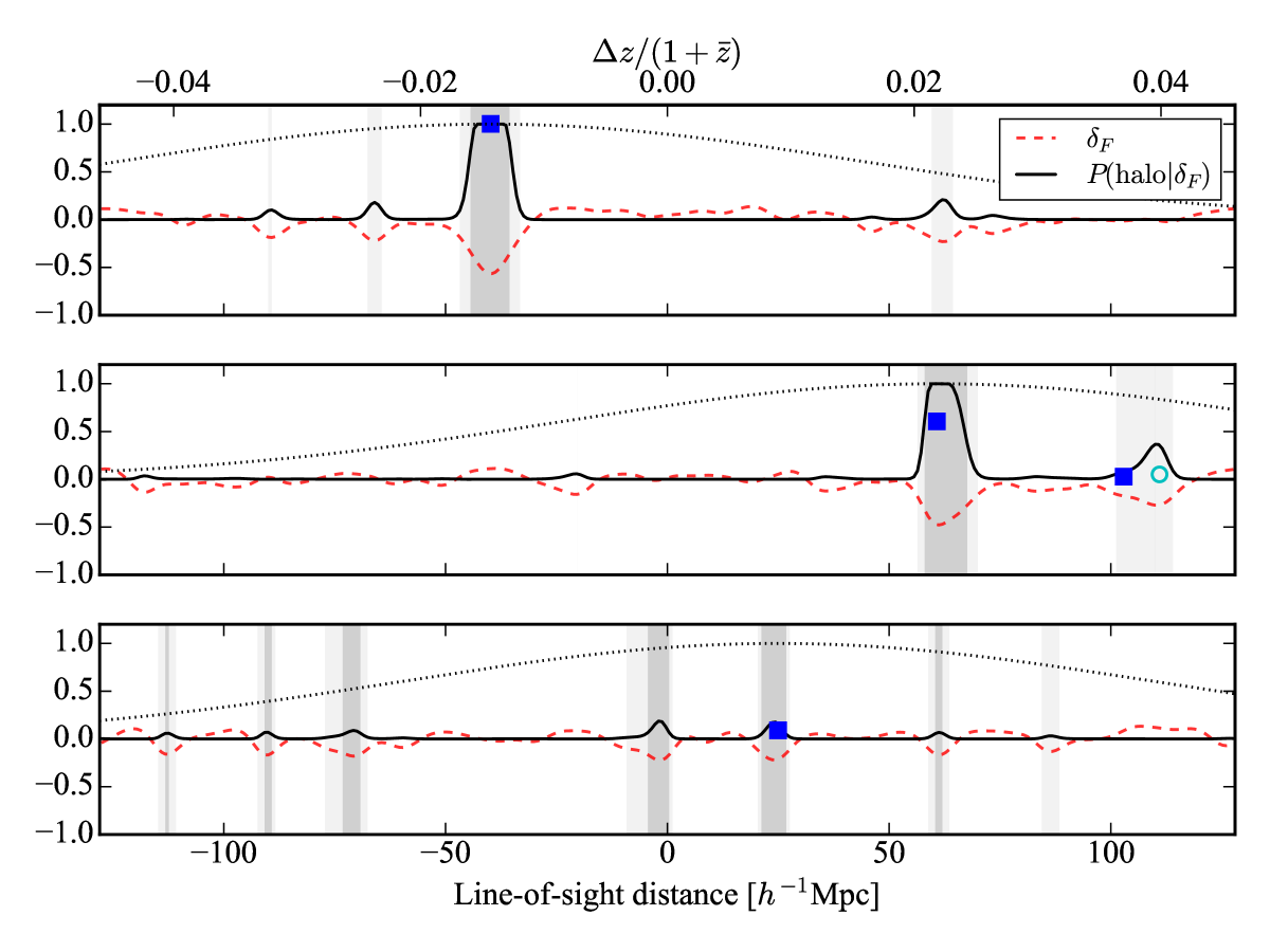
Figure 1: Three sample lines-of-sight through the simulation, showing the Ly$\alpha$ flux (smoothed with a $2.5\,h^{-1}$Mpc Gaussian; red dashed), the probability of the halo being at each position (black solid; normalized to peak at unity in the top panel) and the locations of halos ($M>10^{12}\,h^{-1}M_{\odot}$) within $r<0.5\,h^{-1}$Mpc (solid blue squares) or $0.5\,h^{-1}\mathrm{Mpc}<r<1\,h^{-1}\mathrm{Mpc}$ (open cyan circles) of the line-of-sight. The bottom $x$-axis gives the (comoving) distance while the upper panel shows the equivalent redshift offset from the central redshift $\bar{z}=2.5$ of the skewer. Shaded regions show credible redshift regions (highest posterior density intervals) predicted from $p(z)$, assuming 90 per cent (light grey) or 68 per cent (dark grey) confidence level. The vertical offset of the squares and circles representing the halos is proportional to the logarithm of their mass minus 12. We have plotted skewers passing through the most massive (top; $10^{14}\,h^{-1}M_{\odot}$), $100^{\rm th}$ most massive (middle; $1.6\times 10^{13}\,h^{-1}M_{\odot}$) and $10,000^{\rm th}$ (bottom; $1.5\times 10^{12}\,h^{-1}M_{\odot}$) in the simulation at $z=2.5$. In the lower panel the significance of the detection is low, and the large number of peaks is because there are many regions along the skewer where the flux density is similar to that where the true halo resides. The dotted lines show a Gaussian of width $0.03$ in $\Delta z/(1+\bar{z})$ as an indication of how well a good photometric redshift would constrain $p(z)$.

We have estimated the conditional probability of seeing a halo (more massive than $10^{12}\,h^{-1}M_{\odot}$) given the smoothed Ly$\alpha$ flux directly from the simulations. Along any line of sight we have the smoothed Ly$\alpha$ flux field, $\delta_{F}$. To estimate the probability that a given galaxy (halo) will lie at a given redshift we use Bayes theorem. Specifically we know the distribution of $\delta_{F}$ in the simulation, and we know the distribution of $\delta_{F}$ at the halo locations. Then

$$P({\rm halo}|\delta_{F})=\frac{P(\delta_{F}|{\rm halo})}{P(\delta_{F})}$$ (1)

In the simulations we can estimate this as the ratio of two histograms: First, the histogram of the flux density in the vicinity of massive halos; second, the histogram of the flux density over the whole simulated volume. The result is a monotonically decreasing function of $\delta_{F}$ which can be well fit by a Gaussian (as expected from the arguments above)

$$P({\rm halo}|\delta_{F})\propto e^{-a\delta_{F}-b\delta_{F}^{2}}$$ (2)

with two parameters ($a$ and $b$) aside from the normalization. To obtain this fit we compute the histogram ratio (1) from our simulations using all halos more massive than $10^{12}\,h^{-1}M_{\odot}$ and the flux density interpolated to a $320^{3}$ grid and smoothed with a Gaussian kernel $W_{R}(r)=\exp[-r^{2}/2R^{2}]$ with smoothing scale $R=2.5\,h^{-1}$Mpc. This gives $a=32.3$ and $b=37.1$ if we restrict the fit to smoothed flux values $\delta_{F}>-0.6$ that are present in the simulation.

Our procedure to predict the redshift PDF for galaxies given the flux along their lines of sight is thus as follows. Estimate the smoothed Ly$\alpha$ flux field, as described in Lee et al. (2014b); Stark et al. (2015a). Along the line of sight to each galaxy, compute $p(z)=P\left({\rm halo}|\delta_{F}(z)\right)$ using Eq. (2) with the best-fit values for $a$ and $b$ quoted above. This redshift PDF along the line of sight of each galaxy is the final output of our method.

4 Results

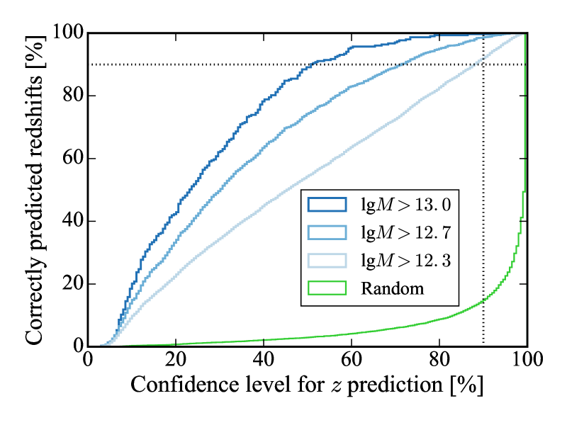
Figure 2: Cumulative fraction of correctly predicted halo redshifts as a function of the confidence level used to select credible redshift regions. This quantifies the error rate of predicted halo redshifts. The plot is obtained as follows: For each halo we compute $p(z)$ along the line of sight using Eq. (2). We then ask what is the lowest confidence level $x$ that we would have to choose so that the credible redshift region based on that confidence level includes the true halo redshift. If the halo is in a high confidence region, this value $x$ would be very small. If the halo is in a low likelihood region we would need a very conservative confidence level (high $x$) for the credible redshift region to contain the halo and this region would encompass most of the probability. The plot shows a cumulative histogram of confidence levels $x$ obtained from all halos above a certain mass (see legend). The vertical axis therefore corresponds to the fraction $y$ of halos for which the confidence level $x$ specified on the horizontal axis is good enough to correctly predict the redshift of $y$ per cent of the halos. The random curve is obtained by putting halos in random locations.

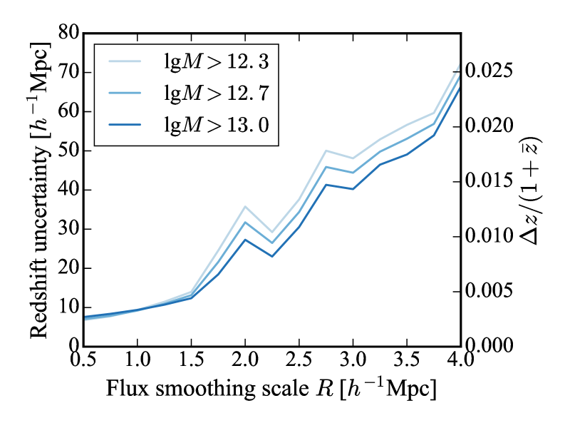
Figure 3: Uncertainty of predicted line-of-sight position or redshift, as a function of flux smoothing scale $R$. Specifically, we define the redshift uncertainty as the total width of $90$ per cent credible intervals for predicted redshifts averaged over all skewers containing at least one halo above the minimum mass specified in the legend. If the predicted $p(z)$ is multi-modal, we quote the summed width of all disconnected intervals (not the distance between $p(z)$ peaks).

Fig. 1 gives three examples of redshift PDFs obtained from the simulation. The three skewers were chosen to be the lines of sight to the most massive, $100^{\rm th}$ most massive and $10,000^{\rm th}$ most massive halos in the simulation, with masses ranging from $10^{14}\,h^{-1}M_{\odot}$ to $10^{12}\,h^{-1}M_{\odot}$. The dashed red line shows the flux while the solid black line shows $p(z)$ (normalized to peak at unity in the top panel). The squares and circles show the positions of halos within $0.5$ and $1\,h^{-1}$Mpc (comoving) of the line of sight, with vertical position indicating their mass. The dotted line shows a Gaussian (normalized to peak at unity) centered at the true position of the halo with width $\Delta z/(1+z)=0.03$, comparable to a good photo-$z$. Clearly including prior photo-$z$ information could serve to eliminate possible peaks in the distribution, corresponding to matter overdensities, which are far from the photo-$z$-determined position.

The upper panel shows that massive halos are very well localized by this technique. Such halos are likely to be tracing protocluster regions at $z=2.5$. The middle panel shows that lines of sight can cross multiple overdensities (e.g. crossing multiple filaments or protocluster regions along the line of sight) and thus $p(z)$ can have more than one peak. This is different from the very low $z$ case (Aragon-Calvo et al., 2015), where there are very few filaments or overdense regions within the survey to cause confusion. In the lower panel we show the difficulties in finding lower mass halos. As Table 1 shows, the abundance of lower mass halos is less sensitive to overdensities measured on $2.5\,h^{-1}$Mpc scales and such halos do not produce a large (smoothed) flux decrement. Thus only a very weak peak is seen at the true location of the halo, and similar peaks are seen at many other locations.

In Fig. 2 we show a summary statistic for the error rate of the predicted photo-$z$s for all of the lines of sight to halos above $2\times 10^{12}\,h^{-1}M_{\odot}$ in the simulation at $z=2.5$. The plot shows the fraction of halos whose redshift is correctly predicted, i.e. the fraction of halos whose true redshift is within the credible redshift region determined from the redshift PDF $p(z)$ computed with Eq. (2) (corresponding to grey regions in Fig. 1). This is shown as a function of the confidence level used to predict these credible redshift regions. As we can see, for halos above $10^{13}\,h^{-1}M_{\odot}$, 90 per cent of the halos lie within the 50-per-cent-confidence-level credible region (i.e. smaller than $1\,\sigma$ for a Gaussian), while only 3 per cent of randomly placed objects do. The situation is less good for lower mass halos, but still far better than random. To further decrease the error rate, we can choose a more conservative confidence level. For example, if we choose to believe the 90-per-cent-confidence-level credible regions, 99.5 per cent of the halos above $10^{13}\,h^{-1}M_{\odot}$, 98.5 per cent of the halos above $5\times 10^{12}\,h^{-1}M_{\odot}$, and 92 per cent of the halos above $2\times 10^{12}\,h^{-1}M_{\odot}$ are predicted correctly. By selecting regions more likely to host massive halos the flux field is drastically improving photo-$z$s.

Although a more conservative confidence level lowers the error rate of predicted halo redshifts, it comes at the cost of increasing the redshift uncertainty by broadening the credible redshift regions. This can be seen in Fig. 1, where the conservative 90-per-cent-confidence-level credible regions (light grey) are broader than those for the less conservative 68 per cent confidence level (dark grey). For our fiducial flux smoothing scale of $R=2.5\,h^{-1}$Mpc we find that the total width of the 90 per cent credible region is $30-40\,h^{-1}$Mpc depending on halo mass. This is roughly the scale of large voids at the high redshifts we are probing. This redshift uncertainty corresponds to $\Delta z/(1+\bar{z})\simeq 0.01$ at $\bar{z}=2.5$, which is significantly better than typical photo-$z$ uncertainties (see Section 1).

Further improvements are possible if we had access to the flux smoothed on smaller scales. We demonstrate this in Fig. 3, which shows the redshift uncertainty given by the total width of the credible region as a function of the flux smoothing scale $R$. With high-resolution flux fields smoothed on $R\sim 1\,h^{-1}$Mpc the redshift uncertainty could be reduced to $10\,h^{-1}$Mpc, while the redshift error rate is essentially independent of the flux smoothing scale (not shown). Longer and more expensive observations to obtain such high-resolution flux fields could thus tighten redshift credible regions by a factor of a few, without increasing the error rate of the redshift predictions (see Lee et al., 2014a, for a discussion of the observational requirements). This would be important for mapping the cosmic web and for environmental studies.

A potential caveat of our method is that the Ly$\alpha$ forest only traces about $400\,$Mpc along the line of sight, so that a galaxy could have higher (lower) redshift than the highest (lowest) redshift for which we have any flux information. Our method might then make a false positive mistake by erroneously assigning a redshift inside the region traced by the Ly$\alpha$ forest. In our simulation, fewer than $10$ per cent of the galaxies that are located at higher or lower redshift than the region traced by the Ly$\alpha$ forest would be (erroneously) given a significant redshift PDF inside the region traced by the Ly$\alpha$ forest. Of course this can be reduced further by trusting only the very highest peaks of the redshift PDF.

5 Future directions

There are numerous improvements that one could imagine to our simple method. First, we have treated all halos (above $10^{12}\,h^{-1}M_{\odot}$) in the same manner. If we knew in advance that a galaxy or its hosting halo was particularly massive we could tune our selection to further improve the performance by focusing on the most extremely overdense regions. We tested this in simulations by calibrating the conditional probability to find a halo given some flux using only halos above $10^{12.5}\,h^{-1}M_{\odot}$ or $10^{13}\,h^{-1}M_{\odot}$. For the same halos, this tightens the total width of credible redshift intervals, but it also leads to a higher fraction of objects outside the high-confidence interval. Usually the redshift error remains small, and it is outside the confidence interval because that interval shrinks so much. Whether this is an improvement depends on the ultimate application and should be studied more quantitatively in the future.

Second, we have not included information about the shape of the cosmic web in our analysis. Lee & White (2016) showed that Ly$\alpha$ forest tomography is capable of classifying the observed volume into voids, sheets, filaments and knots with high fidelity. This could improve our recovery further, e.g. by assigning massive galaxies a higher probability to reside in knots rather than filaments or sheets. As a simple first step in that direction, we characterize different structures of the cosmic web by smoothing the flux on two different smoothing scales, noting that generically both smoothed flux fields should peak for clusters, whereas only the high-resolution flux field might peak if a filament or sheet crosses the sightline. Based on this intuition we generalize our algorithm to use the conditional probability of finding a halo given the flux smoothed on two different smoothing scales, $\delta_{F}$ and $\delta_{F}^{\prime}$:

$$P({\rm halo}|\delta_{F},\delta_{F}^{\prime})=\frac{P(\delta_{F},\delta_{F}^{\prime}|{\rm halo})}{P(\delta_{F},\delta_{F}^{\prime})}.$$ (3)

We compute this in simulations as a ratio of 2d histograms and fit this with a multivariate Gaussian of the form

$$P({\rm halo}|\delta_{F},\delta_{F}^{\prime})\propto e^{-a\delta_{F}-a^{\prime}\delta_{F}^{\prime}-b\delta_{F}^{2}-b^{\prime}\delta_{F}^{\prime 2}-c\delta_{F}\delta_{F}^{\prime}}.$$ (4)

We find that this slightly improves the total widths of credible redshift intervals and the error rate, at the cost of making the method somewhat more complicated. It is possible that including the measured shear could further improve the performance of the method, though properly characterizing the multivariate probability distribution becomes more difficult. Another possibility for improvement might be to increase the integration time of spectra, which would give higher resolution along the line of sight at the expense of observing fewer sightlines at fixed total observation time, effectively reducing the resolution perpendicular to the line of sight. We have not attempted to implement these ideas here, as the simplest method is already performing quite well.

Finally, we have treated each galaxy separately whereas one could imagine a simultaneous recovery of the $p(z)$ for the entire population. Such a procedure is closer in spirit to the one in Jasche & Wandelt (2012) and may yield dividends. Such a forward modeling approach would allow us to take into account the effects of redshift space distortions, bias and the cosmic web using theoretical expectations of how galaxies and the IGM behave in a model based on gravitational instability. This method can also be combined with traditional photo-z’s and alternative redshift estimation techniques like the ones presented in Aragon-Calvo et al. (2015) and in our paper.

Another interesting question is related to observational programs for photo-$z$ calibration. Typically, accurate spectra are measured for all galaxies within the field of interest. In contrast, with our method one could imagine measuring only spectra for the brightest background galaxies, and then using tomographic information from the Ly$\alpha$ forest along the line of sight to calibrate photo-$z$s for multiple galaxies along the line of sight – independent of the galaxy spectral type or whether it has prominent spectral lines. From a single background galaxy spectrum one could then calibrate photo-$z$s in the whole $400$Mpc region along the line of sight. Based on the halo mass dependence of our results this should work best with very massive background halos.

6 Conclusions

Determining the redshift of large numbers of cosmological objects is one of the most difficult problems in observational cosmology. In this paper we have shown that a smoothed map of the intergalactic medium, obtained from spectra of distant galaxies, can be used to improve the redshift accuracy of galaxies and AGN within hundreds of Mpc of the source. This method works because in hierarchical structure formation the halos which host galaxies and AGN preferentially live in the overdense regions with small volume filling fraction.

Our method is extremely simple, once a map of the IGM has been obtained. We use a simple Gaussian form for $p({\rm halo}|\delta_{F})$ to transform the observed flux perturbation, $\delta_{F}$, into a redshift PDF along the line-of-sight to any galaxy. This process can be repeated galaxy by galaxy. Since the mapping between $\delta_{F}$ and $p(z)$ is monotonic, it is easy to account for errors in the IGM map.

In the form presented herein, the method works best for the most massive galaxies which live in the most massive halos, which tend to form in rare regions of very negative $\delta_{F}$. For such massive halos the redshift accuracy and error rate are excellent: at our fiducial $2.5\,h^{-1}$Mpc smoothing $\Delta z/(1+z)\simeq 0.01$ and 90 per cent of halos above $10^{13}\,h^{-1}M_{\odot}$ lie within the 68 per cent credible region. Increasing the resolution of the IGM map reduces the redshift uncertainty, while decreasing the resolution increases the uncertainty. Lower mass halos demand a higher signal-to-noise, less smoothed map of the IGM. This is observationally more challenging.

Our method is extremely straightforward, but does not exhaust the information available in IGM tomography. By using more of the available information about the cosmic web, and by performing a global reconstruction rather than by analyzing galaxies one at a time, we expect to be able to work to lower masses and further improve redshift performance. We defer further developments of a global analysis to future work.

We thank Brice Menard and KG Lee for useful discussions. The simulation, mock surveys, and reconstructions discussed in this work were performed at the National Energy Research Scientific Computing Center, a DOE Office of Science User Facility supported by the Office of Science of the U.S. Department of Energy under Contract No. DE-AC02-05CH11231. This research has made use of NASA’s Astrophysics Data System and of the astro-ph preprint archive at arXiv.org.

References

- Aragon-Calvo et al. (2015) Aragon-Calvo M. A., Weygaert R. v. d., Jones B. J. T., Mobasher B., 2015, MNRAS, 454, 463
- Bardeen et al. (1986) Bardeen J. M., Bond J. R., Kaiser N., Szalay A. S., 1986, ApJ, 304, 15
- Cai et al. (2014) Cai Z., Fan X., Bian F., McGreer I. D., Frye B. L., Yang Y., Zabludoff A. I., Zheng Z., 2014, in American Astronomical Society Meeting Abstracts #223. p. 358.21
- Capak et al. (2007) Capak P., et al., 2007, ApJ Suppl., 172, 99
- Caucci et al. (2008) Caucci S., Colombi S., Pichon C., Rollinde E., Petitjean P., Sousbie T., 2008, MNRAS, 386, 211
- Cole & Kaiser (1989) Cole S., Kaiser N., 1989, MNRAS, 237, 1127
- Dahlen et al. (2013) Dahlen T., et al., 2013, ApJ, 775, 93
- Hildebrandt et al. (2010) Hildebrandt H., et al., 2010, A&A, 523, A31
- Ilbert et al. (2013) Ilbert O., et al., 2013, A&A, 556, A55
- Jasche & Wandelt (2012) Jasche J., Wandelt B. D., 2012, MNRAS, 425, 1042
- Kovač et al. (2010) Kovač K., et al., 2010, ApJ, 708, 505
- Laigle et al. (2016) Laigle C., et al., 2016, ApJ Suppl., 224, 24
- Lee & White (2016) Lee K.-G., White M., 2016, preprint, (arXiv:1603.04441)
- Lee et al. (2014a) Lee K.-G., Hennawi J. F., White M., Croft R. A. C., Ozbek M., 2014a, ApJ, 788, 49
- Lee et al. (2014b) Lee K.-G., et al., 2014b, ApJL, 795, L12
- Lee et al. (2016) Lee K.-G., et al., 2016, ApJ, 817, 160
- Meiksin & White (2001) Meiksin A., White M., 2001, MNRAS, 324, 141
- Mo & White (1996) Mo H. J., White S. D. M., 1996, MNRAS, 282, 347
- Moster et al. (2013) Moster B. P., Naab T., White S. D. M., 2013, MNRAS, 428, 3121
- Muzzin et al. (2013) Muzzin A., et al., 2013, ApJ, 777, 18
- Peacock (1999) Peacock J. A., 1999, Cosmological Physics
- Planck Collaboration et al. (2014) Planck Collaboration et al., 2014, A&A, 571, A16
- Press & Schechter (1974) Press W. H., Schechter P., 1974, ApJ, 187, 425
- Rakic et al. (2011) Rakic O., Schaye J., Steidel C. C., Rudie G. C., 2011, MNRAS, 414, 3265
- Rau et al. (2015) Rau M. M., Seitz S., Brimioulle F., Frank E., Friedrich O., Gruen D., Hoyle B., 2015, MNRAS, 452, 3710
- Rorai et al. (2013) Rorai A., Hennawi J. F., White M., 2013, ApJ, 775, 81
- Sánchez et al. (2014) Sánchez C., et al., 2014, MNRAS, 445, 1482
- Scoville et al. (2007) Scoville N., et al., 2007, ApJ Suppl., 172, 1
- Stark et al. (2015a) Stark C. W., White M., Lee K.-G., Hennawi J. F., 2015a, MNRAS, 453, 311
- Stark et al. (2015b) Stark C. W., Font-Ribera A., White M., Lee K.-G., 2015b, MNRAS, 453, 4311
- Tinker & Conroy (2009) Tinker J. L., Conroy C., 2009, ApJ, 691, 633