Room	Mic.	Dimensions	Source		5-channel	3-channel	8-channel
Name	Pos.	(L, W, H)	Position	Look dir.	Cruciform	Mobile	Linear array
Office 1	1	(3.32, 4.83, 2.95)	(2.06, 1.04, 1.19)	90	(2.66, 2.14, 1.19)	(2.29, 2.15, 1.19)	(1.92, 2.14, 1.19)
Office 1	2	(3.32, 4.83, 2.95)	(2.06, 1.04, 1.19)	90	(2.49, 3.69, 1.19)	(2.15, 3.69, 1.19)	(1.79, 3.67, 1.19)
Office 2	1	(3.22, 5.1, 2.94)	(1.41, 1.73, 1.19)	90	(1.25, 2.81, 1.19)	(1.25, 2.62, 1.19)	(0.84, 2.78, 1.19)
Office 2	2	(3.22, 5.1, 2.94)	(1.41, 1.73, 1.19)	90	(2.25, 4.35, 1.19)	(2.05, 4.16, 1.19)	(1.58, 4.16, 1.19)
Meeting Room 1	1	(6.61, 5.11, 2.95)	(1.39, 1.26, 1.19)	0	(2.74, 0.48, 1.19)	(2.74, 0.82, 1.19)	(2.74, 1.14, 1.19)
Meeting Room 1	2	(6.61, 5.11, 2.95)	(1.39, 1.26, 1.19)	0	(3.96, 0.52, 1.19)	(3.96, 0.85, 1.19)	(3.96, 1.14, 1.19)
Meeting Room 2	1	(10.3, 9.07, 2.63)	(4.65, 4.07, 1.19)	180	(3, 4.39, 1.19)	(3, 3.99, 1.19)	(3, 3.59, 1.19)
Meeting Room 2	2	(10.3, 9.07, 2.63)	(4.65, 4.07, 1.19)	180	(2, 4.39, 1.19)	(2, 3.99, 1.19)	(2, 3.59, 1.19)
Lecture Room 1	1	(6.93, 9.73, 3)	(3.65, 3.73, 1.19)	180	(2.81, 3.84, 1.19)	(2.8, 3.44, 1.19)	(2.89, 3.04, 1.19)
Lecture Room 1	2	(6.93, 9.73, 3)	(3.65, 3.73, 1.19)	180	(1.07, 3.92, 1.19)	(1.07, 3.52, 1.19)	(1.07, 3.12, 1.19)
Lecture Room 2	1	(13.6, 9.29, 2.94)	(6.03, 3.14, 1.19)	180	(5.09, 5.87, 1.19)	(5.09, 5.47, 1.19)	(5.09, 5.07, 1.19)
Lecture Room 2	2	(13.6, 9.29, 2.94)	(6.03, 3.14, 1.19)	180	(3.93, 5.87, 1.19)	(3.93, 5.47, 1.19)	(3.93, 5.07, 1.19)
Building Lobby	1	(4.47, 5.13, 3.18)	(1.98, 0.61, 1.19)	90	(2.69, 2.02, 1.19)	(2.33, 2, 1.19)	(1.95, 2.03, 1.19)
Building Lobby	2	(4.47, 5.13, 3.18)	(1.98, 0.61, 1.19)	90	(2.62, 3.51, 1.19)	(2.25, 3.49, 1.19)	(1.86, 3.54, 1.19)

Table 2: Room dimensions, source, microphone and fan positions continued

1.2.2 Talker positions for babble noise

Table 1.2.2 provides each of the talker positions used to produce the babble noise. The $z$ coordinates are not provided since these were not captured. However, the talkers were seated and their mouths were situated at approximately the same height as the microphone arrays which were all at $1.19\text{\,}\mathrm{m}$ above the floor.

Table 3: Talker positions used to produce babble noise

1.2.3 Distances and look directions

Table 1.2.3 provides the source-microphone distances and DoA in spherical coordinates, whilst Table 1.2.3 provides the fan-microphone distances and DoA in spherical coordinates.

Table 4: Source–microphone distances and DoA in spherical coordinates

Table 5: Fan–microphone distances and DoA

1.3 Taxonomy of algorithms submitted

There were three main classes of algorithms submitted to the ACE Challenge:

1. ABC (ABC);

2. SFM (SFM);

3. MLMF (MLMF).

The ABC approaches derive the estimate for the acoustic parameter directly from the signal without requiring any prior information. Bias compensation may be performed in order to account for noise or specific aspects of the source material. An example of this is the maximum likelihood method [Lollmann2010] which directly produces the T60 estimate.

The SFM approaches estimate a parameter from a signal that is correlated with the acoustic parameter to be estimated, and then apply a mapping function to give the acoustic parameter estimate. An example of this is the SDD method which determines NSV (NSV) from STFT bins and then applies a mapping to obtain the T60.

The MLMF approaches typically use many features of the source material to train a neural network which then estimates the acoustic parameter from the features of a test signal. An example of this is the NIRA (NIRA) [Parada2015] algorithm.

There were no hybrid approaches submitted to the ACE Challenge although several participants applied noise reduction to the source signals before performing parameter estimation.

Algorithms are further classified as being either providing an estimate in FB2 (FB2), in frequency bands, or SB.

1.4 Results

The participating institutions in the ACE challenge along with their respective algorithms are listed in Table 6 in order of appearance of their algorithms in the results tables.

Table 6: ACE Challenge participants

Participant	Algorithms submitted (see results tables)
	T60	DRR
Federal University of Rio de Janeiro	A	$\alpha$
FAU (FAU)	B, C, D, E
Imperial College London	F, G	v, w, x, y, z
Fraunhofer IDMT	H, I, J, K, L, M, N, O	p, q, r, s, t, u
MuSAELab	O, P, Q, R, S, T, U, V, W	0, 1, 2, 3, 4, 5, 6, 7, 8, 9
Nuance Communications Inc.	X, Y, Z	k, l, m
Microsoft Research	a, b
University of Auckland/NTT		f, g, h, i, j
ANU (ANU)		n

For the fullband tasks the results are presented as box plots where there is a box shown for each algorithm. Both single and multi-channel algorithms are shown in the same figures and tables. On each box in the box plot, the central notch is the median, the edges of the box are the 25 and 75 percentiles, the whiskers extend to the most extreme data points not considered outliers. Boxes are colour-coded according to algorithm class: ABC: yellow; MLMF: cyan; SFM: green.

Outliers are plotted individually. The algorithms are identified on the box plot by a single character which corresponds to the character in the table after the figure. The results are sorted by the research group which achieved the highest correlation coefficient in the results across all noises and SNR in fullband. For the T60 fullband task, the last three algorithms are those compared in Gaubitch et al. [Gaubitch2012] and are included as baselines to enable the progress made in blind T60 estimation since 2012 to be assessed. Similarly, for the DRR fullband task, Jeub et al. [Jeub2011] is included as the last algorithm since this was a freely available estimator prior to the ACE Challenge. The correlation coefficient for each algorithm is plotted as a black cross in the same column as the algorithm. The value is provided on the right hand $y$-axis.

A table of numerical results is also provided following each figure which also provides the legend for the algorithm identifiers, A, B, C, etc. The columns in the table are as follows:

1. Ref., the identifier for each algorithm used on the $x$-axis of the preceding figure;

2. Algorithm, the name used by the respective ACE Challenge participant to refer to their algorithm;

3. Class, the class of algorithm according to Sec. 1.3;

4. Mic. Config, the microphone configuration of the Evaluation dataset used to test the algorithm. Valid values are Single (1-channel), Chromebook (2-channel), Mobile (3-channel), Crucif (5-channel), Lin8Ch (8-channel), and EM32 (32-channel); Further details of the microphone configurations can be found in [Eaton2015a];

5. Bias, the mean error in the results. ; Let $X=[x_{0},x_{1},\dots x_{N-1}]$ equal the set of $N$ ground truth T60 and DRR measurements, and let $\hat{X}$ equal the set of estimated results defined similarly. Then

   $$\text{Bias}=\frac{1}{N}\sum\limits^{N-1}_{n=0}\hat{x_{n}}-x_{n};$$ (1)

6. MSE, the mean squared error in the estimation results defined as

   $$\text{MSE}=\frac{1}{N}\sum\limits^{N-1}_{n=0}(\hat{x_{n}}-x_{n})^{2}.$$ (2)

7. $\rho$, the Pearson correlation coefficient between the estimated and the ground truth results defined as

   $$\rho=\frac{E\{\hat{X}X\}-E\{\hat{X}\}E\{X\}}{\sqrt{(E\{\hat{X^{2}}\}-E\{\hat{X}\}^{2})(E\{X^{2}\}-E\{X\}^{2})}},$$ (3)

   where $E\{\cdot\}$ is the mathematical expectation;

8. RTF, the real-time factor, the total computation time divided by the total duration of all processed speech files. All implementations were in Matlab except for those marked with a ^† which used Matlab for feature extraction and C++ for the machine learning-based mapping, and those marked with a ^‡ which were implemented entirely in C++.

By considering the bias, MSE, and $\rho$, it is possible to determine how well the estimator works. For example, an estimator with a low bias and MSE might simply be giving an estimate close to the median for every speech file. However, by examining the $\rho$, it will be possible to distinguish between such an algorithm, which will have a low correlation, and a better algorithm which is more accurately estimating the parameter concerned which will have a higher correlation. The RTF (RTF) is useful for determining whether the algorithm has practical applications requiring low computational complexity such as hearing aids and mobile devices.

For the frequency-dependent tasks, a box plot is provided per algorithm with each box representing the performance in a particular frequency band. Frequency dependent algorithms have also been included in the fullband plots. Where those algorithms themselves produce a fullband estimate, this has been used directly as in the case of the DENBE (DENBE) [Eaton2015c] and Particle Velocity [Chen2015] algorithms. Where no fullband estimate is produced, a fullband estimate was obtained by taking the mean of the results over the $400$ to $1250\text{\,}\mathrm{Hz}$ frequency bands as in the case of the Model-based subband RTE [Lollmann2015] algorithm as recommended in ISO 3382 [ISO_3382].

2 Overall results summary

2.1 Fullband T60 estimation overall results

The overall results for fullband T60 estimation are shown in Fig. 2 and Table 2.1.

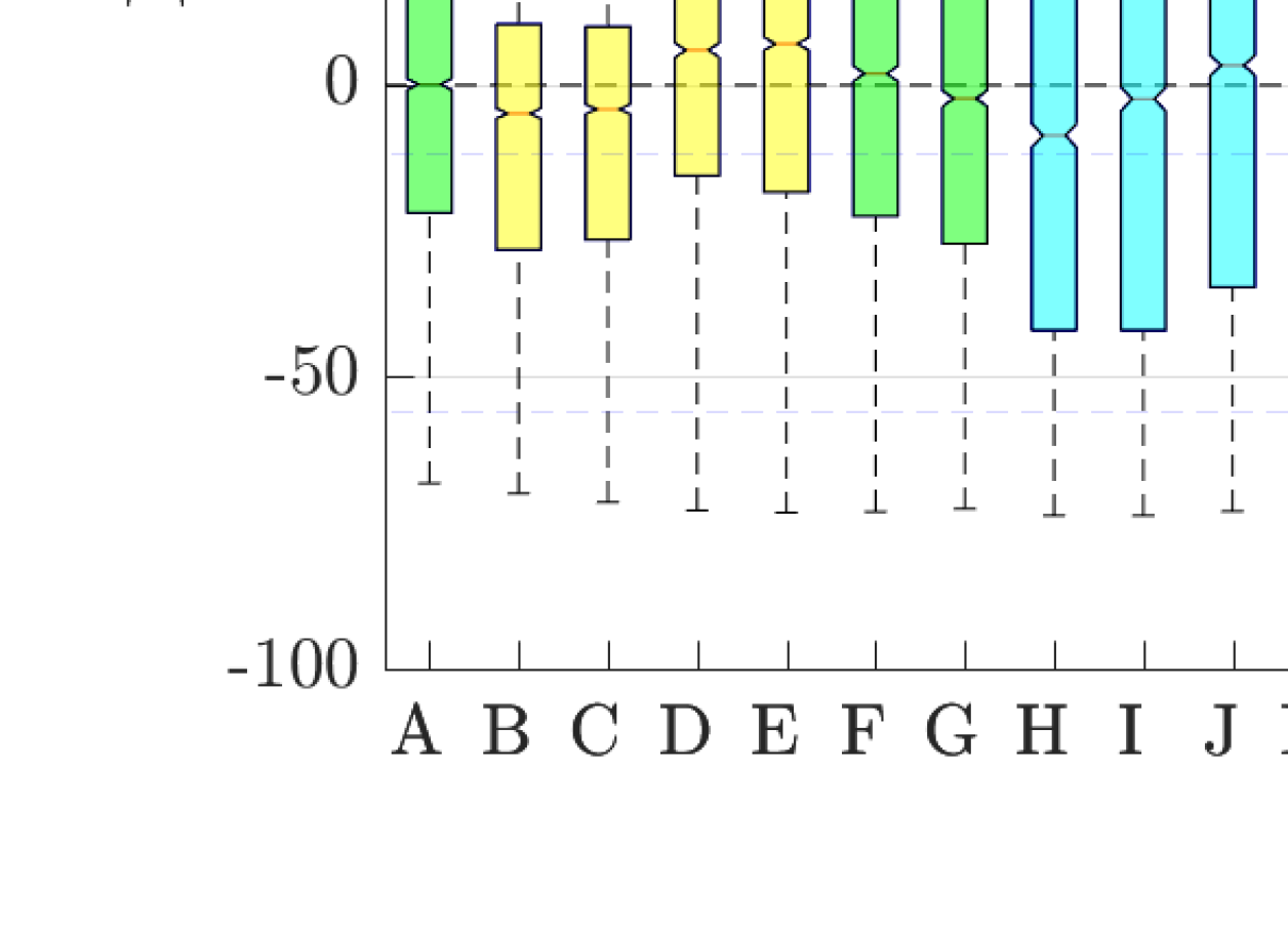
Figure 2: Fullband T60 estimation error in all noises for all SNR

Table 7: T60 estimation algorithm performance in all noises for all SNR

2.2 Fullband DRR estimation overall results

The overall results for fullband DRR estimation are shown in Fig. 3 and Table 2.2.

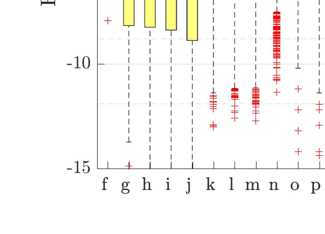
Figure 3: Fullband DRR estimation error in all noises for all SNR

Table 8: DRR estimation algorithm performance in all noises for all SNR

Ref.	Algorithm	Class	Mic. Config.	Bias	MSE	$\rho$	RTF
f	PSD est. in beamspace, bias comp. [Hioka2015]	ABC	Mobile	1.07	8.14	0.577	0.757
g	PSD est. in beamspace (Raw) [Hioka2015]	ABC	Mobile	-5.9	41.8	0.577	3.17
h	PSD est. in beamspace v2 [Hioka2015]	ABC	Mobile	-5.7	43	0.41	0.844
i	PSD est. by twin BF [Hioka2012]	ABC	Mobile	-5.71	44.9	0.362	0.614
j	Spatial Covariance in matrix mode [Hioka2011]	ABC	Mobile	-5.37	61.2	0.244	0.627
k	NIRAv2 [Parada2015]	MLMF	Single	-1.85	14.8	0.558	0.899†
l	NIRAv3 [Parada2015]	MLMF	Single	-1.62	14.7	0.515	0.899†
m	NIRAv1 [Parada2015]	MLMF	Single	-1.64	15	0.507	0.899†
n	Particle velocity [Chen2015]	ABC	EM32	-2.38	10.4	0.449	0.134
o	Multi-layer perceptron [Xiong2015]	MLMF	Single	-1.14	15.9	0.405	0.0578‡
p	Multi-layer perceptron P2 [Xiong2015]	MLMF	Single	-1.52	16.1	0.507	0.0578‡
q	Multi-layer perceptron P2 [Xiong2015]	MLMF	Chromebook	-2.43	13.6	0.265	0.0589‡
r	Multi-layer perceptron P2 [Xiong2015]	MLMF	Mobile	-1.67	15	0.403	0.0556‡
s	Multi-layer perceptron P2 [Xiong2015]	MLMF	Crucif	-1.5	16	0.503	0.0569‡
t	Multi-layer perceptron P2 [Xiong2015]	MLMF	Lin8Ch	-3.64	25.7	0.314	0.0618‡
u	Multi-layer perceptron P2 [Xiong2015]	MLMF	EM32	-2.22	14.6	0.325	0.0576‡
v	DENBE no noise reduction [Eaton2015]	ABC	Chromebook	-6.04	51.2	0.308	0.0323
w	DENBE spectral subtraction [Eaton2015c]	ABC	Chromebook	-4.25	34.1	0.314	0.0589
x	DENBE spec. sub. Gerkmann [Eaton2015]	ABC	Chromebook	-4.01	32.8	0.303	0.0477
y	DENBE filtered subbands [Eaton2015c]	ABC	Chromebook	-4.01	32.8	0.303	0.775
z	DENBE FFT derived subbands [Eaton2015c]	ABC	Chromebook	-4.01	32.8	0.303	0.0449
0	NOSRMR (NOSRMR) Sec. 2.2. [Senoussaoui2015]	SFM	Chromebook	-5.1	34.3	0.269	1.04
1	OSRMR (OSRMR) Sec. 2.2. [Senoussaoui2015]	SFM	Chromebook	-3.71	20.6	0.259	0.829
2	NOSRMR Sec. 2.2. [Senoussaoui2015]	SFM	Mobile	-4.47	32	0.148	1.58
3	OSRMR Sec. 2.2. [Senoussaoui2015]	SFM	Mobile	-3.28	22.2	0.116	1.26
4	NOSRMR Sec. 2.2. [Senoussaoui2015]	SFM	Crucif	-4.05	31.1	0.0814	2.62
5	OSRMR Sec. 2.2. [Senoussaoui2015]	SFM	Crucif	-2.88	22.3	0.0616	2.09
6	NOSRMR Sec. 2.2. [Senoussaoui2015]	SFM	Single	-4.16	33.9	-0.0841	0.54
7	OSRMR Sec. 2.2. [Senoussaoui2015]	SFM	Single	-4.24	34.6	-0.0815	0.446
8	Per acoust. band SRMR Sec. 2.5. [Senoussaoui2015]	SFM	Single	-0.9	22.8	0.00192	0.578
9	Temporal dynamics [Falk2009]	SFM	Single	-11.4	147	0.0815	0.082
$\alpha$	QA Reverb [Prego2015]	SFM	Single	2.51	23.6	0.0576	0.391
$\beta$	Blind est. of coherent-to-diffuse energy ratio [Jeub2011]	ABC	Chromebook	-12.1	162	0.305	0.019

2.2.1 Fullband T60 estimation results by parameter

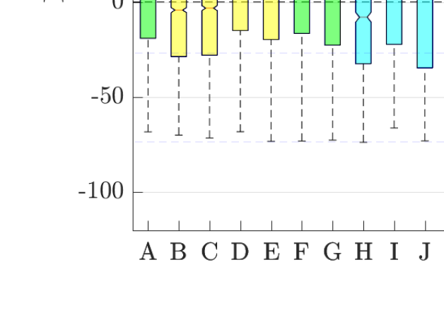
(a)

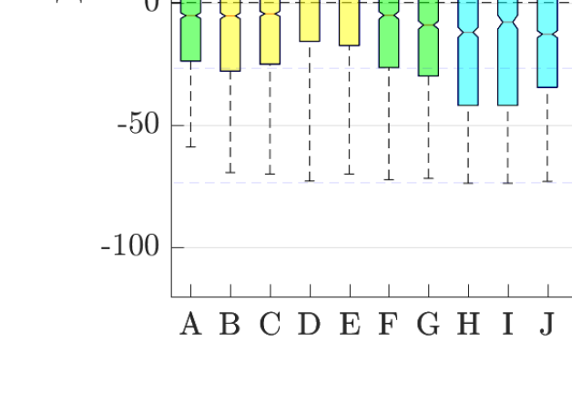
(b)

Figure 4: FB2 T60 estimation error in all noises and all SNR for a) female talkers and b) male talkers

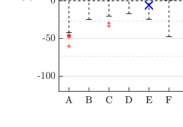
(a)

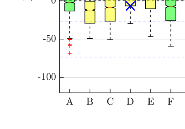
(b)

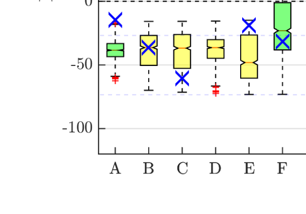
(c)

Figure 5: Single channel FB2 T60 estimation error in all noises and all SNR for a) T60 $<$$0.43\text{\,}\mathrm{s}$ b) $0.43\leq$T60 $<$ $0.75\text{\,}\mathrm{s}$ and c) T60 $\geq$ $0.75\text{\,}\mathrm{s}$. Observe that $\rho<0$ for all except algorithm D

(a)

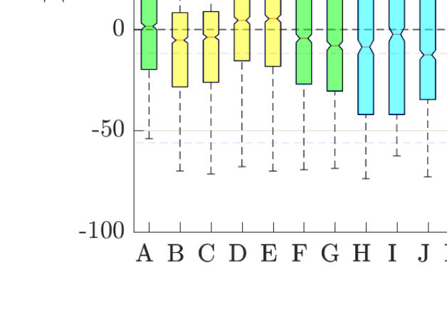
(b)

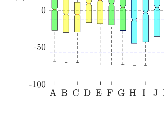
(c)

Figure 6: FB2 T60 estimation error in all noises at a), $18\text{\,}\mathrm{dB}$ SNR, b), $12\text{\,}\mathrm{dB}$ SNR, and c) $-1\text{\,}\mathrm{dB}$ SNR

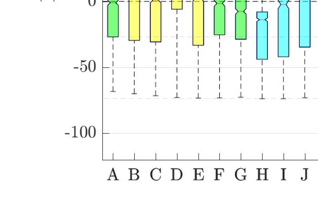
(a)

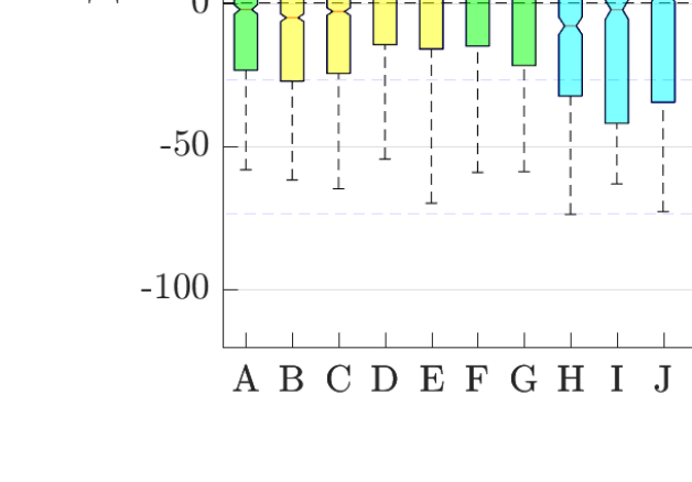
(b)

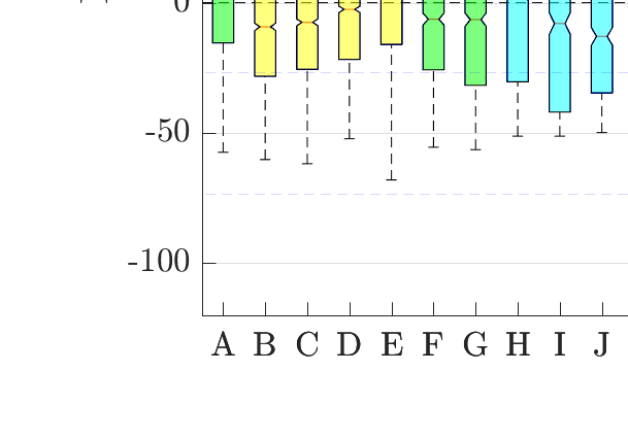
(c)

Figure 7: FB2 T60 estimation error in all noises and all SNR for a) utterance length $<$$5\text{\,}\mathrm{s}$ b) utterance length $<$ $15\text{\,}\mathrm{s}$ and c) utterance length $\geq$ $15\text{\,}\mathrm{s}$

2.2.2 Fullband DRR estimation results by parameter

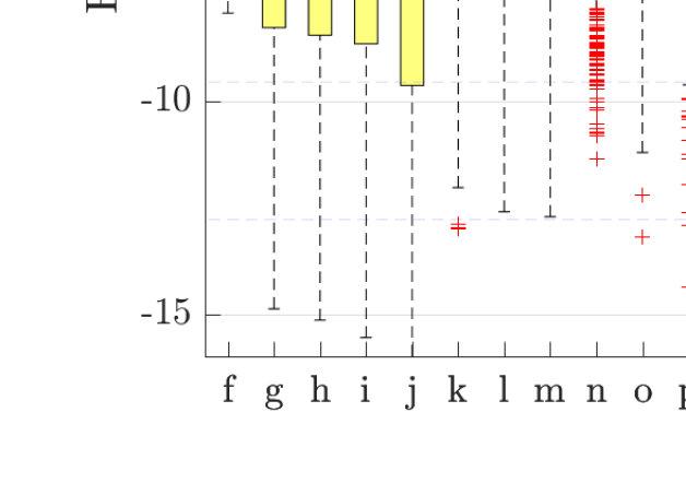
(a)

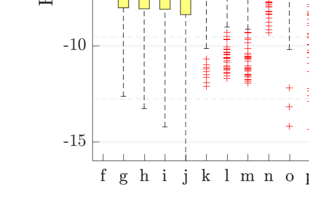
(b)

Figure 8: FB2 DRR estimation error in all noises and all SNR for a) female talkers and b) male talkers

(a)

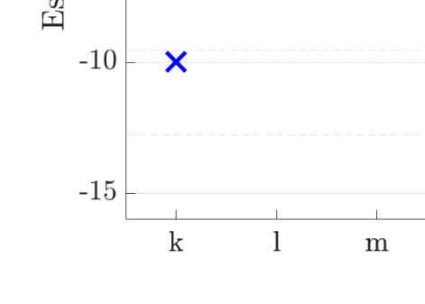
(b)

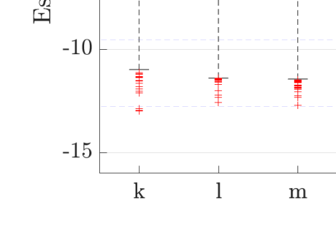
(c)

Figure 9: Single channel FB2 DRR estimation error in all noises and all SNR for a) DRR $<$$2\text{\,}\mathrm{dB}$ b) $2\leq$DRR $<$ $5\text{\,}\mathrm{dB}$ and c) DRR $\geq$ $5\text{\,}\mathrm{dB}$

(a)

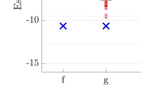
(b)

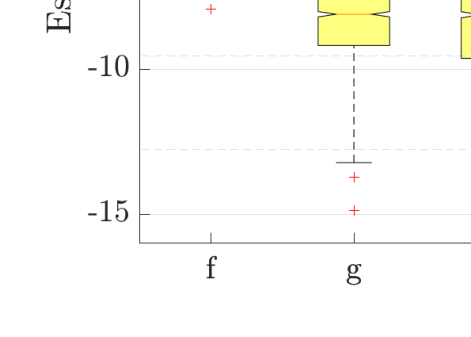
(c)

Figure 10: Mobile (3-channel) FB2 DRR estimation error in all noises and all SNR for a) DRR $<$$2\text{\,}\mathrm{dB}$ b) $2\leq$DRR $<$ $5\text{\,}\mathrm{dB}$ and c) DRR $\geq$ $5\text{\,}\mathrm{dB}$. Note that for b) there are strong negative correlations for all algorithms

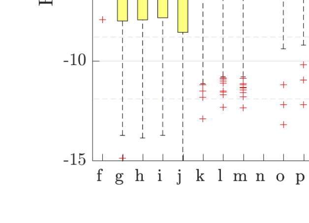
(a)

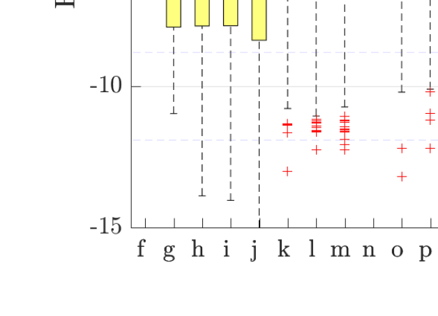
(b)

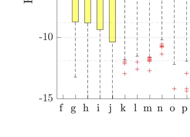
(c)

Figure 11: FB2 DRR estimation error in all noises at a), $18\text{\,}\mathrm{dB}$ SNR, b), $12\text{\,}\mathrm{dB}$ SNR, and c) $-1\text{\,}\mathrm{dB}$ SNR

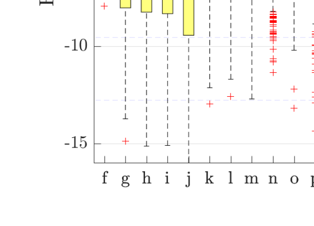
(a)

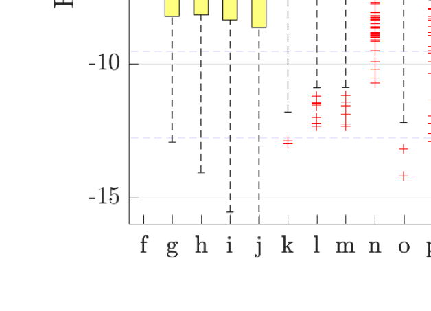
(b)

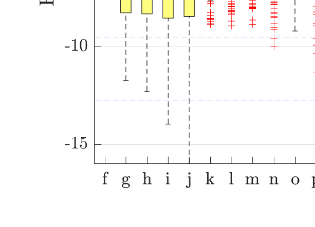
(c)

Figure 12: FB2 DRR estimation error in all noises and all SNR for a) utterance length $<$$5\text{\,}\mathrm{s}$ b) utterance length $<$ $15\text{\,}\mathrm{s}$ and c) utterance length $\geq$ $15\text{\,}\mathrm{s}$

3 T60 estimation results

3.1 Fullband T60 estimation results by noise type

3.1.1 Ambient noise

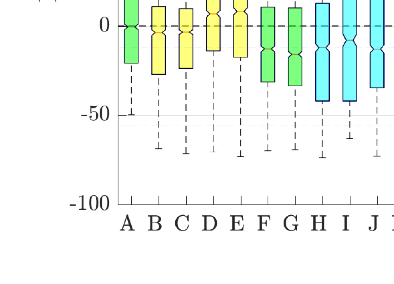
Figure 13: Fullband T60 estimation error in ambient noise for all SNR

Table 9: T60 estimation algorithm performance in ambient noise for all SNR

3.1.2 Babble noise

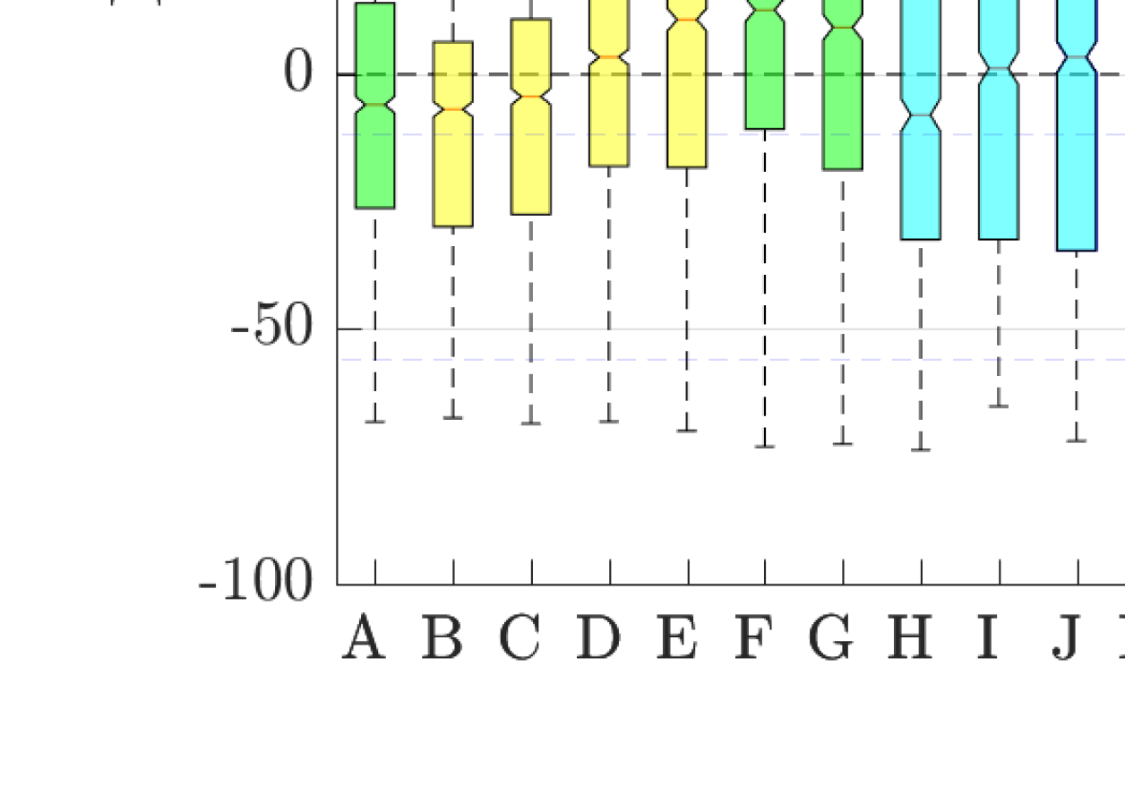
Figure 14: Fullband T60 estimation error in babble noise for all SNR

Table 10: T60 estimation algorithm performance in babble noise for all SNR

3.1.3 Fan noise

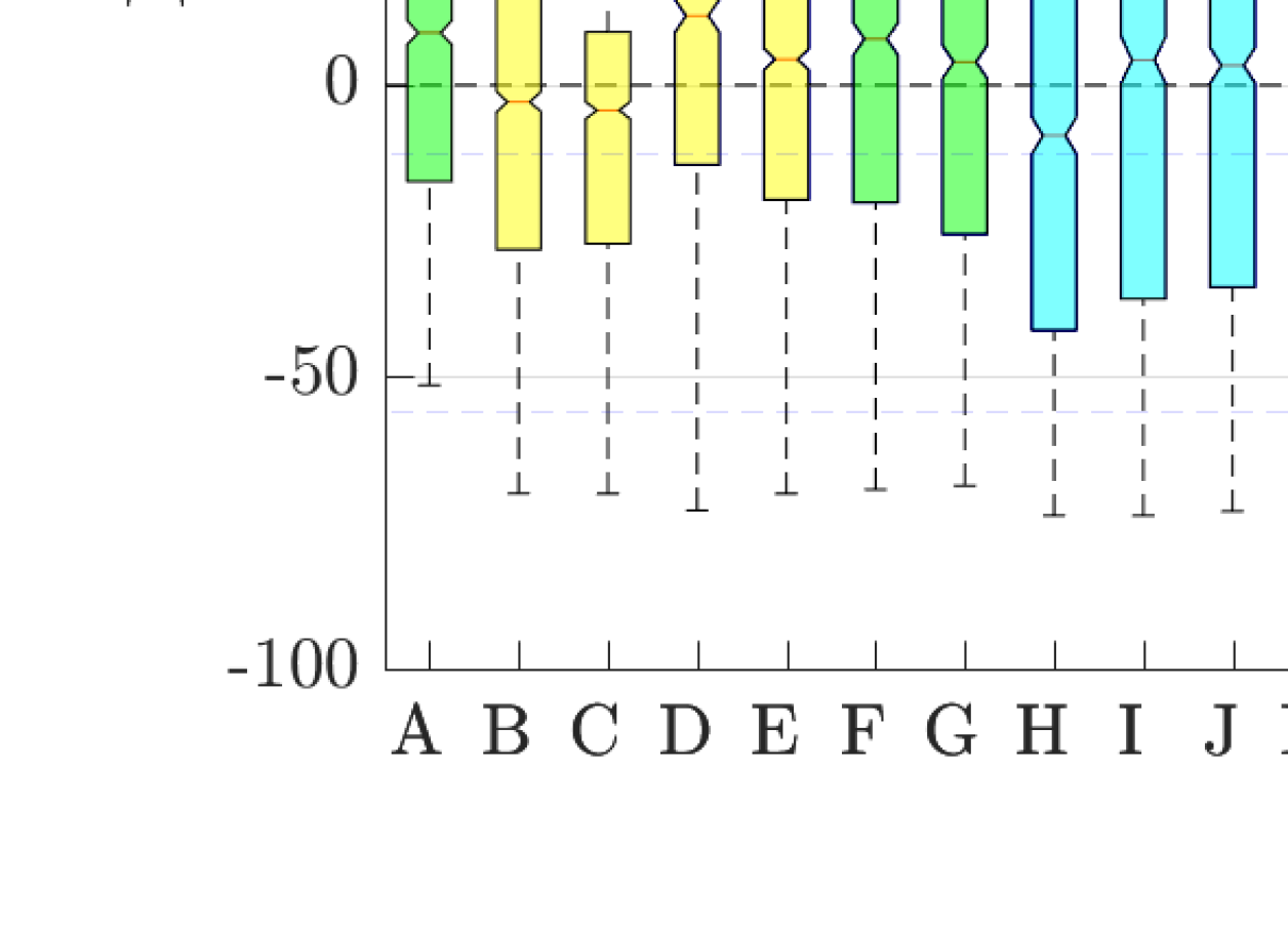
Figure 15: Fullband T60 estimation error in fan noise for all SNR

Table 11: T60 estimation algorithm performance in fan noise for all SNR

3.2 Fullband T60 estimation results by noise type and SNR

3.2.1 Ambient noise at $18\text{\,}\mathrm{dB}$ SNR

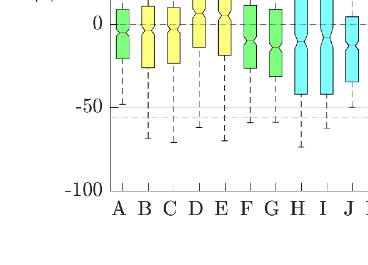
Figure 16: Fullband T60 estimation error in ambient noise at $18\text{\,}\mathrm{dB}$ SNR

Table 12: T60 estimation algorithm performance in ambient noise at $18\text{\,}\mathrm{dB}$ SNR

3.2.2 Ambient noise at $12\text{\,}\mathrm{dB}$ SNR

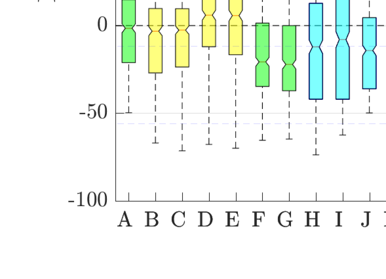
Figure 17: Fullband T60 estimation error in ambient noise at $12\text{\,}\mathrm{dB}$ SNR

Table 13: T60 estimation algorithm performance in ambient noise at $12\text{\,}\mathrm{dB}$ SNR

3.2.3 Ambient noise at $-1\text{\,}\mathrm{dB}$ SNR

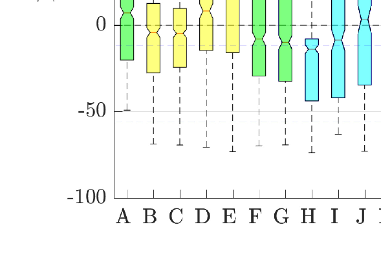
Figure 18: Fullband T60 estimation error in ambient noise at $-1\text{\,}\mathrm{dB}$ SNR

Table 14: T60 estimation algorithm performance in ambient noise at $-1\text{\,}\mathrm{dB}$ SNR

3.2.4 Babble noise at $18\text{\,}\mathrm{dB}$ SNR

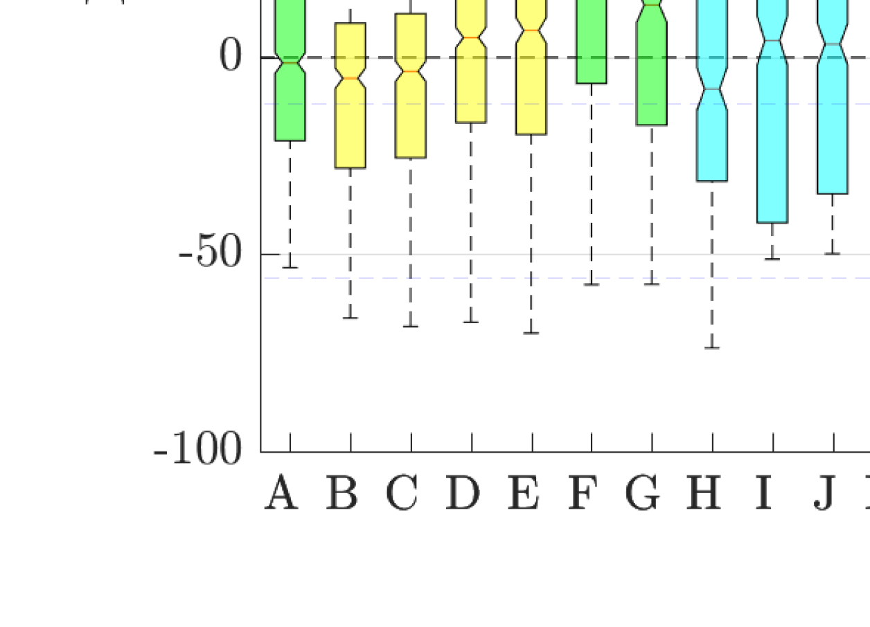
Figure 19: Fullband T60 estimation error in babble noise at $18\text{\,}\mathrm{dB}$ SNR

Table 15: T60 estimation algorithm performance in babble noise at $18\text{\,}\mathrm{dB}$ SNR

3.2.5 Babble noise at $12\text{\,}\mathrm{dB}$ SNR

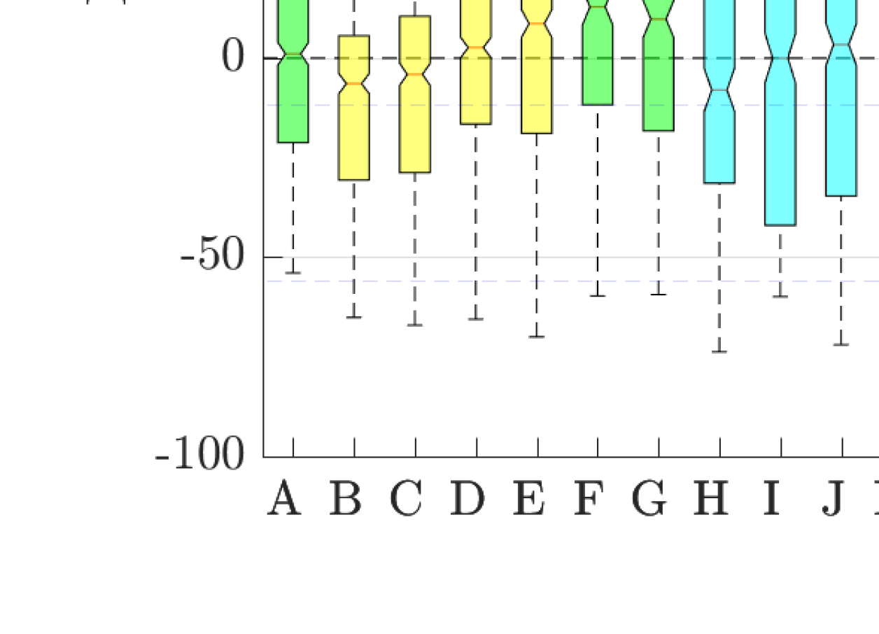
Figure 20: Fullband T60 estimation error in babble noise at $12\text{\,}\mathrm{dB}$ SNR

Table 16: T60 estimation algorithm performance in babble noise at $12\text{\,}\mathrm{dB}$ SNR

3.2.6 Babble noise at $-1\text{\,}\mathrm{dB}$ SNR

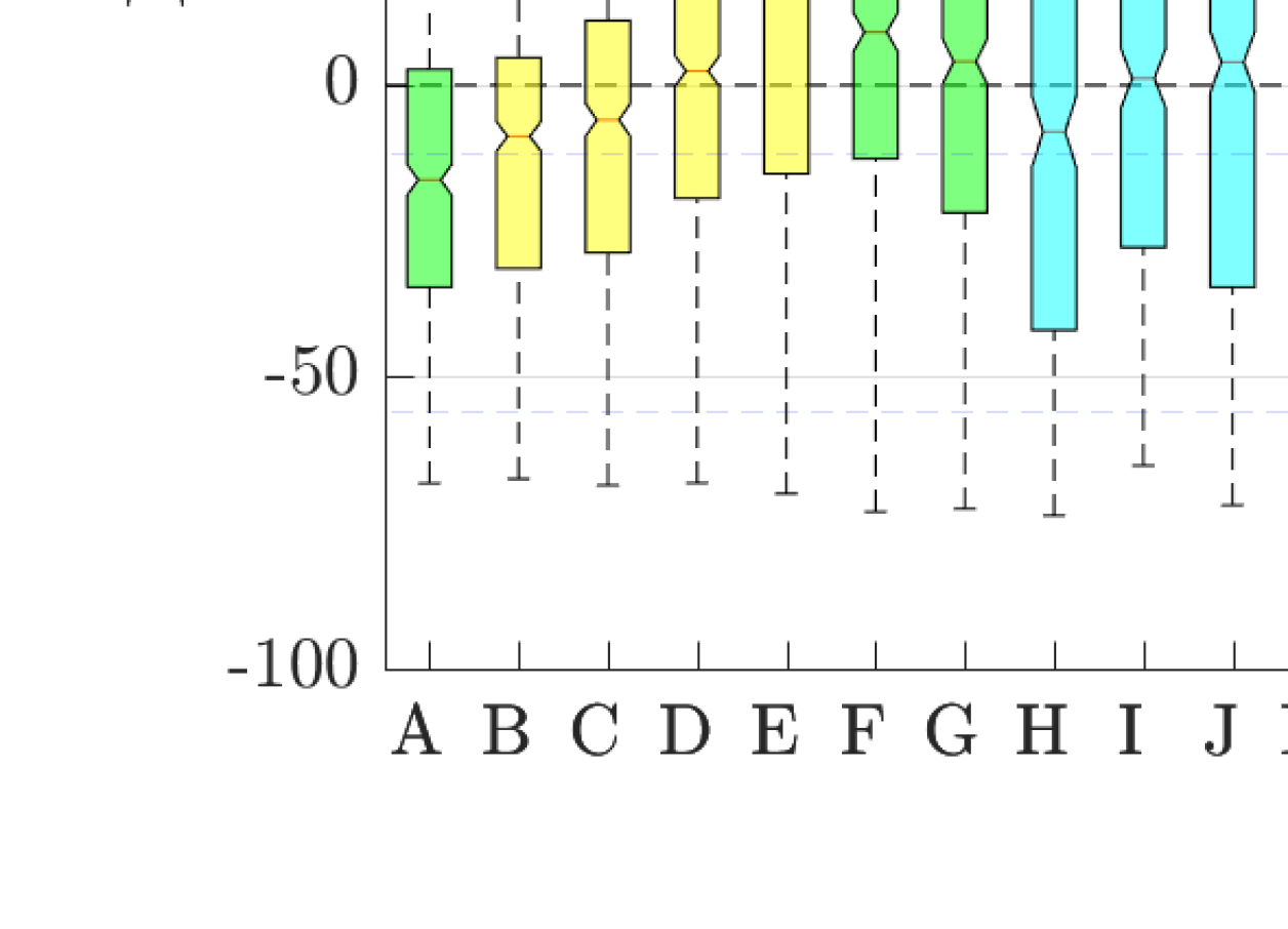
Figure 21: Fullband T60 estimation error in babble noise at $-1\text{\,}\mathrm{dB}$ SNR

Table 17: T60 estimation algorithm performance in babble noise at $-1\text{\,}\mathrm{dB}$ SNR

3.2.7 Fan noise at $18\text{\,}\mathrm{dB}$ SNR

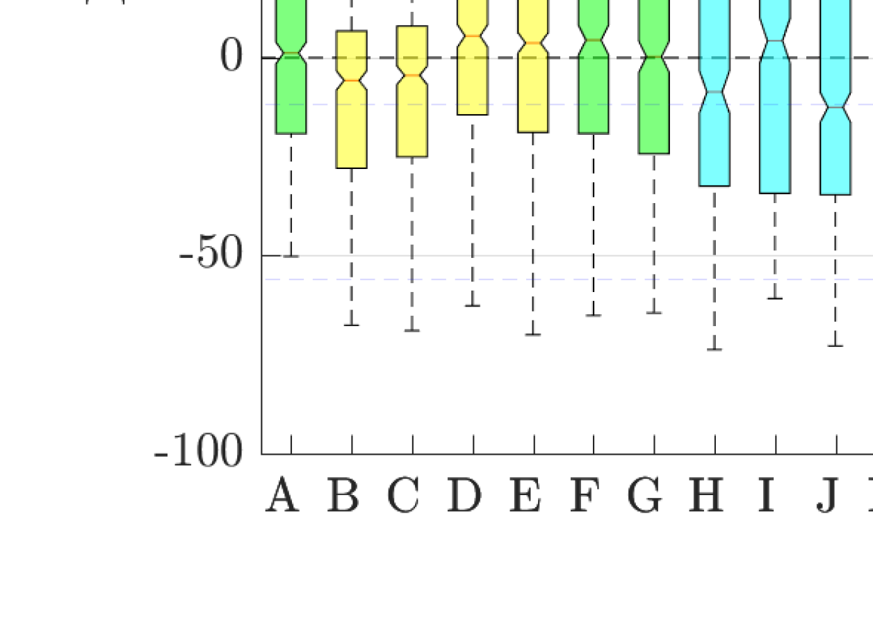
Figure 22: Fullband T60 estimation error in fan noise at $18\text{\,}\mathrm{dB}$ SNR

Table 18: T60 estimation algorithm performance in fan noise at $18\text{\,}\mathrm{dB}$ SNR

3.2.8 Fan noise at $12\text{\,}\mathrm{dB}$ SNR

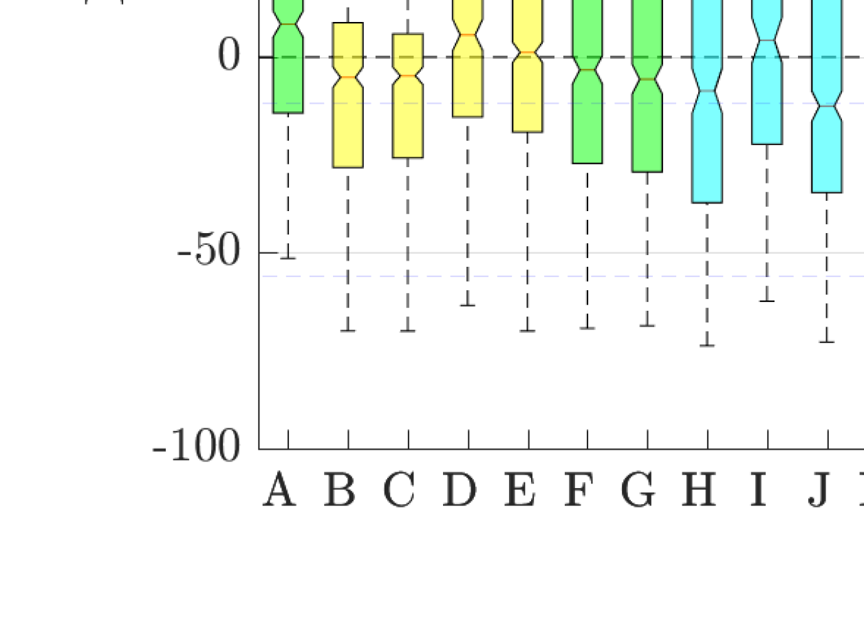
Figure 23: Fullband T60 estimation error in fan noise at $12\text{\,}\mathrm{dB}$ SNR

Table 19: T60 estimation algorithm performance in fan noise at $12\text{\,}\mathrm{dB}$ SNR

3.2.9 Fan noise at $-1\text{\,}\mathrm{dB}$ SNR

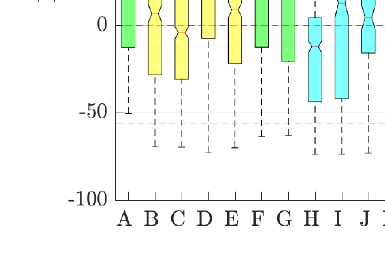
Figure 24: Fullband T60 estimation error in fan noise at $-1\text{\,}\mathrm{dB}$ SNR

Table 20: T60 estimation algorithm performance in fan noise at $-1\text{\,}\mathrm{dB}$ SNR

3.3 Frequency-dependent T60 estimation results

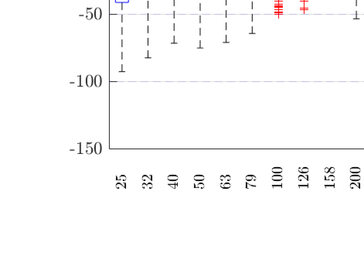
Figure 25: Frequency-dependent T60 estimation error in all noises for all SNR for algorithm Model-based SB RTE [Lollmann2015]

Table 21: T60 estimation algorithm performance for all noises for all SNR

3.4 Frequency-dependent T60 estimation results by noise type

3.4.1 Ambient noise

Figure 26: Frequency-dependent T60 estimation error in ambient noise for all SNR for algorithm Model-based SB RTE [Lollmann2015]

Table 22: Frequency-dependent T60 estimation error in ambient noise for all SNR for algorithm Model-based SB RTE [Lollmann2015]

3.4.2 Babble noise

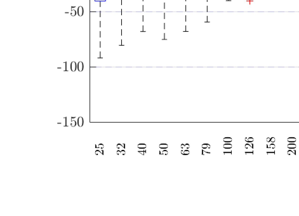
Figure 27: Frequency-dependent T60 estimation error in babble noise for all SNR for algorithm Model-based SB RTE [Lollmann2015]

Table 23: Frequency-dependent T60 estimation error in babble noise for all SNR for algorithm Model-based SB RTE [Lollmann2015]

3.4.3 Fan noise

Figure 28: Frequency-dependent T60 estimation error in fan noise for all SNR for algorithm Model-based SB RTE [Lollmann2015]

Table 24: Frequency-dependent T60 estimation error in fan noise for all SNR for algorithm Model-based SB RTE [Lollmann2015]

3.5 Frequency-dependent T60 estimation results by noise type and SNR

3.5.1 Ambient noise at $18\text{\,}\mathrm{dB}$

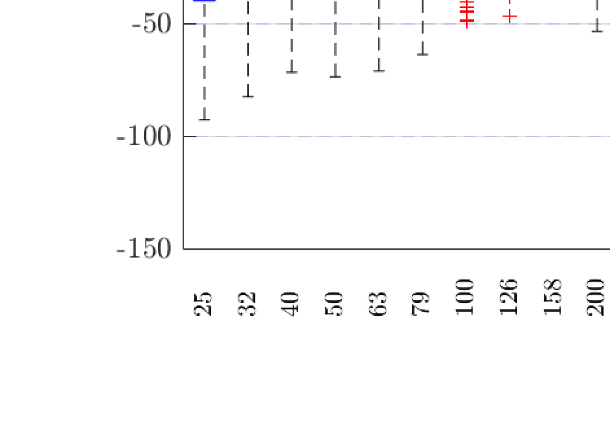
Figure 29: Frequency-dependent T60 estimation error in ambient noise at $18\text{\,}\mathrm{dB}$ SNR for algorithm Model-based SB RTE [Lollmann2015]

Table 25: Frequency-dependent T60 estimation error in ambient noise at $18\text{\,}\mathrm{dB}$ SNR for algorithm Model-based SB RTE [Lollmann2015]

3.5.2 Ambient noise at $12\text{\,}\mathrm{dB}$

Figure 30: Frequency-dependent T60 estimation error in ambient noise at $12\text{\,}\mathrm{dB}$ SNR for algorithm Model-based SB RTE [Lollmann2015]

Table 26: Frequency-dependent T60 estimation error in ambient noise at $12\text{\,}\mathrm{dB}$ SNR for algorithm Model-based SB RTE [Lollmann2015]

3.5.3 Ambient noise at $-1\text{\,}\mathrm{dB}$

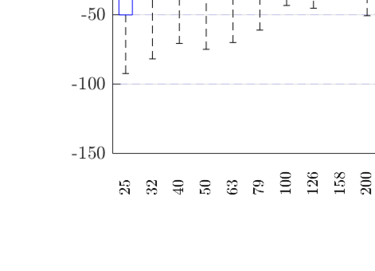
Figure 31: Frequency-dependent T60 estimation error in ambient noise at $-1\text{\,}\mathrm{dB}$ SNR for algorithm Model-based SB RTE [Lollmann2015]

Table 27: Frequency-dependent T60 estimation error in ambient noise at $-1\text{\,}\mathrm{dB}$ SNR for algorithm Model-based SB RTE [Lollmann2015]

3.5.4 Babble noise at $18\text{\,}\mathrm{dB}$

Figure 32: Frequency-dependent T60 estimation error in babble noise at $18\text{\,}\mathrm{dB}$ SNR for algorithm Model-based SB RTE [Lollmann2015]

Table 28: Frequency-dependent T60 estimation error in babble noise at $18\text{\,}\mathrm{dB}$ SNR for algorithm Model-based SB RTE [Lollmann2015]

3.5.5 Babble noise at $12\text{\,}\mathrm{dB}$

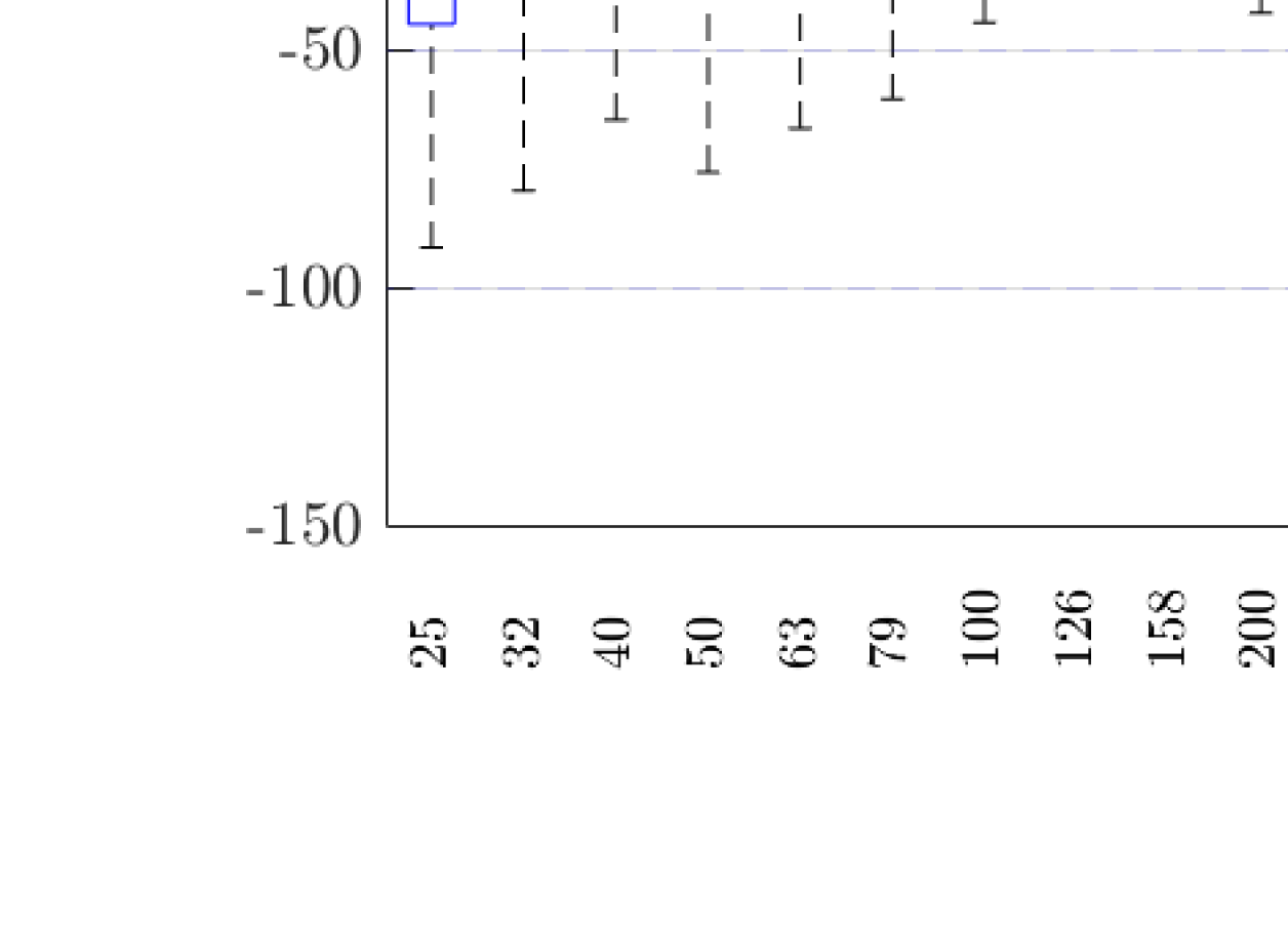
Figure 33: Frequency-dependent T60 estimation error in babble noise at $12\text{\,}\mathrm{dB}$ SNR for algorithm Model-based SB RTE [Lollmann2015]

Table 29: Frequency-dependent T60 estimation error in babble noise at $12\text{\,}\mathrm{dB}$ SNR for algorithm Model-based SB RTE [Lollmann2015]

3.5.6 Babble noise at $-1\text{\,}\mathrm{dB}$

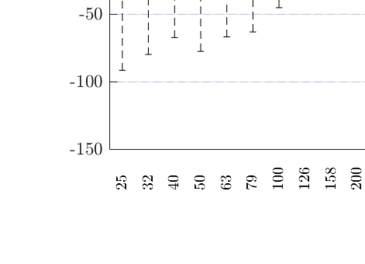
Figure 34: Frequency-dependent T60 estimation error in babble noise at $-1\text{\,}\mathrm{dB}$ SNR for algorithm Model-based SB RTE [Lollmann2015]

Table 30: Frequency-dependent T60 estimation error in babble noise at $-1\text{\,}\mathrm{dB}$ SNR for algorithm Model-based SB RTE [Lollmann2015]

3.5.7 Fan noise at $18\text{\,}\mathrm{dB}$

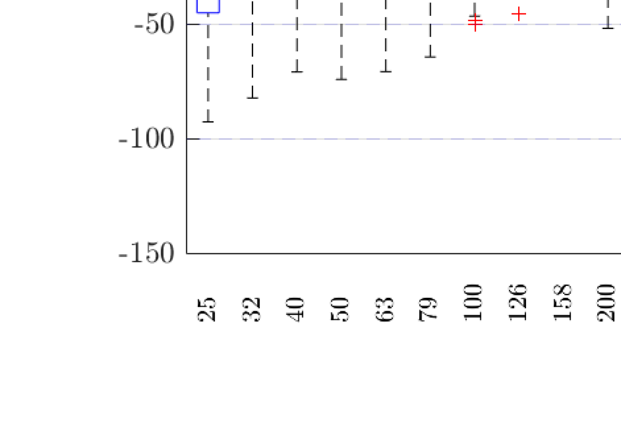
Figure 35: Frequency-dependent T60 estimation error in fan noise at $18\text{\,}\mathrm{dB}$ SNR for algorithm Model-based SB RTE [Lollmann2015]

Table 31: Frequency-dependent T60 estimation error in fan noise at $18\text{\,}\mathrm{dB}$ SNR for algorithm Model-based SB RTE [Lollmann2015]

3.5.8 Fan noise at $12\text{\,}\mathrm{dB}$

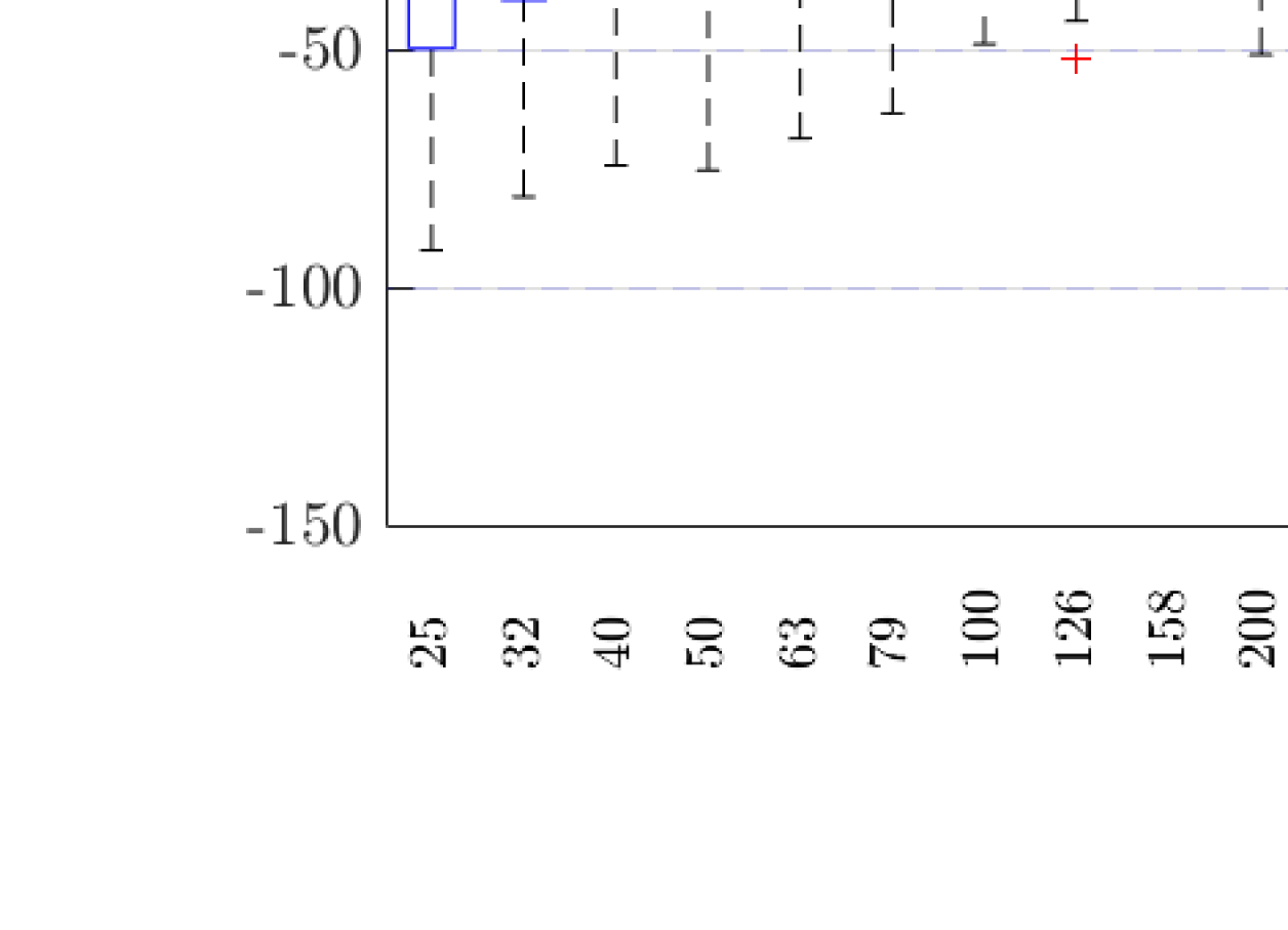
Figure 36: Frequency-dependent T60 estimation error in fan noise at $12\text{\,}\mathrm{dB}$ SNR for algorithm Model-based SB RTE [Lollmann2015]

Table 32: Frequency-dependent T60 estimation error in fan noise at $12\text{\,}\mathrm{dB}$ SNR for algorithm Model-based SB RTE [Lollmann2015]

3.5.9 Fan noise at $-1\text{\,}\mathrm{dB}$

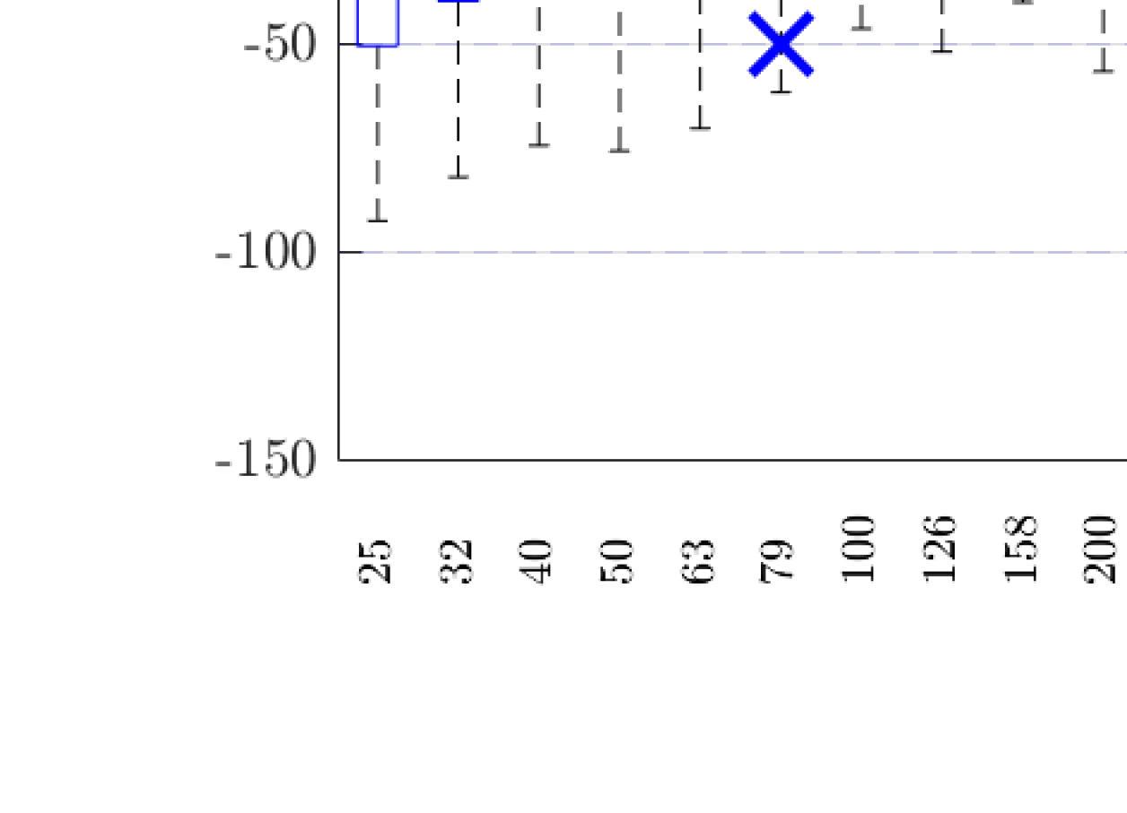
Figure 37: Frequency-dependent T60 estimation error in fan noise at $-1\text{\,}\mathrm{dB}$ SNR for algorithm Model-based SB RTE [Lollmann2015]

Table 33: Frequency-dependent T60 estimation error in fan noise at $-1\text{\,}\mathrm{dB}$ SNR for algorithm Model-based SB RTE [Lollmann2015]