Higher-order expansions of extremes from mixed skew-$t$ distribution

Abstract.  In this paper, we study the asymptotic behaviors of the extreme of mixed skew-t distribution. We considered limits on distribution and density of maximum of mixed skew-t distribution under linear and power normalization, and further derived their higher-order expansions, respectively. Examples are given to support our findings.

Keywords.  Mixed skew-$t$ distribution; Extreme value distribution; Higher order expansions; Power normalization; Linear normalization.

1 Introduction

The skew-$t$ distribution due to Azzalini and Capitanio (2003) can be defined as follows. Let $Y$ and $Z$ be two independent random variables with $Y$ following $\chi^{2}(v)$ with degree of freedom $v$ and $Z$ being a skew-normal random variable with probability density function (pdf)

$$f_{Z}(x)=2\phi(x)\Phi(\beta x)$$

for $x\in\operatorname*{\mathbb{R}}$ and parameter $\beta\in\operatorname*{\mathbb{R}}$, where $\phi(\cdot)$ denote the standard normal pdf and $\Phi(\cdot)$ denotes the standard normal cumulative distribution function (cdf). Define $X=Y/\sqrt{Z/v}$, then $X$ is said to have skew-$t$ distribution, written as $X\sim\operatorname*{ST}_{v}(\beta)$ for short. Azzalini and Capitanio (2003) showed that the pdf of $\operatorname*{ST}_{v}(\beta)$ is

$$f(x)=2t_{v}(x)T_{v+1}\left(\beta x\sqrt{\frac{v+1}{x^{2}+v}}\right),$$ (1.1)

where $t_{v}(\cdot)$ is the pdf of the standard Student’s $t$ distribution with degree of freedom $v$, and $T_{v+1}(\cdot)$ is the cdf of the standard Student’s $t$ distribution with degree of freedom $v+1$. Note that

$$t_{v}(x)=C_{v}\left(1+\frac{x^{2}}{v}\right)^{-\frac{v+1}{2}},$$ (1.2)

where $x\in\operatorname*{\mathbb{R}}$ and $C_{v}=\frac{\Gamma\left(\frac{v+1}{2}\right)}{\Gamma\left(\frac{v}{2}\right)\sqrt{v\pi}}$. It follows from (1.1) and (1.2) that $f\in RV_{-\alpha-1}$ implying $F\in D(\Phi_{\alpha})$, i.e, there exist norming constant $a_{n}>0$ such that

$$\lim_{n\to\infty}F^{n}(a_{n}x)=\Phi_{\alpha}(x)=\exp(-x^{-\alpha}),\;\;x>0,$$ (1.3)

where $F$ is the cdf of skew-t distribution. Here, $g\in RV_{\beta}$ means $\lim_{t\to\infty}g(tx)/g(t)=x^{\beta}$ for $x>0$. Further extremal properties such as distributional expansions of extremes from skew-t distribution, see Peng et al. (2016).

Nowadays finite mixed distribution has received widespread research. Peel and Mclachlan (2000) considered a robust approach by modelling atypical observations by a mixture of Student-t distributions. Frigessi et al.(2002) proposed a dynamic mixture approach to estimate the severity distributions. Dellaportas and Papageorgiou (2006) presented full Bayesian analysis of finite mixtures of multivariate normals with unknown number of components. Cabral et al. (2008) gave a Bayesian approach for modeling heterogeneous data and estimated multimodal densities using mixtures of skew student-t-normal distributions. Sattayatham and Talangtam (2012) modeled motor insurance claims data from Thailand by using a mixture of log-normal distributions. Lin et al. (2007) proposed a robust mixture framework based on the skew-t distribution, and provided EM-type algorithms for iteratively computing maximum likelihood estimates. Frühwrith-Schnatter and Pyne (2010) investigated Bayesian inference for finite mixtures of skew-normal and skew-t distributions, and applied them to modelling non-Gaussian cell populations. Ho and Lin (2010) considered a robust linear mixed skew-t models with application to schizophrenia data. A two-component skew-t mixture model is used to analyze freeway speed data characteristics by Zou and Zhang (2011). For more studies related to the mixed multivariate skew-t distribution, we refer to Lin (2010), Vrbik and McNicholas (2012), Lee and McLachlan (2013, 2014).

The objective of this paper is to study the asymptotic behaviors of extremes of finite mixed skew-t distribution (shortened by $\operatorname*{MSTD}$) under linear and power normalization, respectively. The finite $\operatorname*{MSTD}$ is defined as follows. Let $X_{1},X_{2},\cdots,X_{r}$ be independent random variables with $X_{i}\sim\operatorname*{ST}_{v_{i}}(\beta_{i})$, where $v_{i}>0$ and $\beta_{i}\in\operatorname*{\mathbb{R}}$ for $i=1,2,\cdots,r.$ Without loss of generality we suppose that $v_{1}<v_{2}<\cdots<v_{r}$. Define a new random variable $T$ by

$$T=\left\{\begin{aligned} &X_{1},&\quad\operatorname*{P}(T=X_{1})=p_{1}&\\ &X_{2},&\quad\operatorname*{P}(T=X_{2})=p_{2}&\\ &\vdots&\vdots\quad&\\ &X_{r},&\quad\operatorname*{P}(T=X_{r})=p_{r}&,\end{aligned}\right.$$ (1.4)

where $p_{i}>0$($1\leq i\leq r$) satisfying $\sum_{i=1}^{r}p_{i}=1$. Then $T$ is said to have finite $\operatorname*{MSTD}$ with $r$ components. Denoting by $F_{v,\beta}(x)$ the cdf of a random variable $X\sim\operatorname*{ST}_{v}(\beta)$ and $F(x)$ the cdf of the random variable $T$, we can easily get

$$F(x)=p_{1}F_{v_{1},\beta_{1}}(x)+p_{2}F_{v_{2},\beta_{2}}(x)+\cdots+p_{r}F_{v_{r},\beta_{r}}(x).$$ (1.5)

Contents of this paper are organized as follows. In Section 2, expansion of the distributional tail of $\operatorname*{MSTD}$ shows that extreme value distribution from $\operatorname*{MSTD}$ sample is Fréchet distribution under given linear normalization, implying that under power normalization the extreme value distribution from $\operatorname*{MSTD}$ is $\Phi_{1}(x)$. Higher-order expansions of the cdf and the pdf of extremes from $\operatorname*{MSTD}$ are given in Section 3. Numerate analysis provided in Section 4 compare the asymptotic behaviors under different normalization.

2 Preliminaries

In this section, we provide some primary results related to $\operatorname*{ST}$ and $\operatorname*{MSTD}$. The first one is from Peng et al. (2016).

Lemma 2.1.

Let $F_{v,\beta}(x)$ denote the cdf of the skew-$t$ distribution. For large $x$, we have

$$1-F_{v,\beta}(x)=2C_{v}v^{\frac{v-1}{2}}T_{v+1}(\beta\sqrt{v+1})x^{-v}\left(1+A_{1}x^{-2}+A_{2}x^{-4}+O(x^{-6})\right),$$ (2.1)

where

$$A_{1}=-\frac{C_{v+1}v^{2}\sqrt{v+1}\beta(1+\beta^{2})^{-\frac{v+2}{2}}}{2T_{v+1}(\beta\sqrt{v+1})(v+2)}-\frac{v^{2}(v+1)}{2(v+2)}$$

and

$$A_{2} = \frac{C_{v+1}\sqrt{v+1}\beta(1+\beta^{2})^{-\frac{v+2}{2}}}{T_{v+1}(\beta\sqrt{v+1})}\left[\frac{3v^{2}}{8}+\frac{v^{3}(v-1)}{4(v+2)}-\frac{3v^{2}}{(v+2)(v+4)}-\frac{(v+2)\beta^{2}v^{3}}{8(v+4)(1+\beta^{2})}\right]$$

$$+\frac{v^{2}(v^{2}-1)}{8}+\frac{3v^{2}}{(v+2)(v+4)}+\frac{v^{2}(v-1)}{2(v+2)}.$$

For the distibutional tail behavior of $\operatorname*{MSTD}$, we have the following results.

Lemma 2.2.

Let F(x) be the cdf of random variable $T$, for large $x$ we have

$$1-F(x) = 2p_{1}C_{v_{1}}v_{1}^{\frac{v_{1}-1}{2}}T_{v_{1}+1}(\beta_{1}\sqrt{v_{1}+1})x^{-v_{1}}(1+A_{1}x^{-2}+A_{2}x^{-4}+A_{3}x^{-(v_{2}-v_{1})}$$

$$+A_{4}x^{-(v_{2}-v_{1})-2}+A_{5}x^{-(v_{3}-v_{1})}+O(x^{-\eta}))$$

where $\eta=\min\{6,v_{4}-v_{1},v_{2}-v_{1}+4,v_{3}-v_{1}+2\}$ and

$$A_{1}=-\frac{C_{v_{1}+1}v_{1}^{2}\sqrt{v_{1}+1}\beta_{1}(1+\beta_{1}^{2})^{-\frac{v_{1}+2}{2}}}{2T_{v_{1}+1}(\beta_{1}\sqrt{v_{1}+1})(v_{1}+2)}-\frac{v_{1}^{2}(v_{1}+1)}{2(v_{1}+2)};$$

$$A_{2}=\frac{C_{v_{1}+1}\sqrt{v_{1}+1}\beta_{1}(1+\beta_{1}^{2})^{-\frac{v_{1}+2}{2}}}{T_{v_{1}+1}(\beta_{1}\sqrt{v_{1}+1})}\left[\frac{v_{1}^{3}(v_{1}-1)}{4(v_{1}+2)}+\frac{3v_{1}^{2}}{8}-\frac{3v_{1}^{2}}{(v_{1}+2)(v_{1}+4)}-\frac{(v_{1}+2)\beta_{1}^{2}v_{1}^{3}}{8(v_{1}+4)(1+\beta_{1}^{2})}\right]$$

$$+\frac{v_{1}^{2}(v_{1}^{2}-1)}{8}+\frac{3v_{1}^{2}}{(v_{1}+2)(v_{1}+4)}+\frac{v_{1}^{2}(v_{1}-1)}{2(v_{1}+2)};$$

$$A_{3}=\frac{p_{2}C_{v_{2}}v_{2}^{\frac{v_{2}-1}{2}}T_{v_{2}+1}(\beta_{2}\sqrt{v_{2}+1})}{p_{1}C_{v_{1}}v_{1}^{\frac{v_{1}-1}{2}}T_{v_{1}+1}(\beta_{1}\sqrt{v_{1}+1})};$$

$$A_{4}=-\frac{p_{2}C_{v_{2}}v_{2}^{\frac{v_{2}-1}{2}}T_{v_{2}+1}(\beta_{2}\sqrt{v_{2}+1})}{p_{1}C_{v_{1}}v_{1}^{\frac{v_{1}-1}{2}}T_{v_{1}+1}(\beta_{1}\sqrt{v_{1}+1})}\left(\frac{C_{v_{2}+1}v_{2}^{2}\sqrt{v_{2}+1}\beta_{2}(1+\beta_{2}^{2})^{-\frac{v_{2}+2}{2}}}{2(v_{2}+2)T_{v_{2}+1}(\beta_{2}\sqrt{v_{2}+1})}+\frac{v_{2}^{2}(v_{2}+1)}{2(v_{2}+2)}\right);$$

$$A_{5}=\frac{p_{3}C_{v_{3}}v_{3}^{\frac{v_{3}-1}{2}}T_{v_{3}+1}(\beta_{3}\sqrt{v_{3}+1})}{p_{1}C_{v_{1}}v_{1}^{\frac{v_{1}-1}{2}}T_{v_{1}+1}(\beta_{1}\sqrt{v_{1}+1})}.$$

Proof.

To simplify the proof, we first define two functions $A_{1}(\cdot,\cdot)$ and $A_{2}(\cdot,\cdot)$ as following. For $i=1,\cdots,r,$ define

$$A_{1}(v_{i},\beta_{i})=-\frac{C_{v_{i}+1}v_{i}^{2}\sqrt{v_{i}+1}\beta_{i}(1+\beta_{i}^{2})^{-\frac{v_{i}+2}{2}}}{2(v_{i}+2)T_{v_{i}+1}(\beta_{i}\sqrt{v_{i}+1})}-\frac{v_{i}^{2}(v_{i}+1)}{2(v_{i}+2)}$$

and

$$A_{2}(v_{i},\beta_{i}) = \frac{C_{v_{i}+1}\sqrt{v_{i}+1}\beta(1+\beta_{i}^{2})^{-\frac{v_{i}+2}{2}}}{T_{v_{i}+1}(\beta\sqrt{v_{i}+1})}$$

$$\times\left[\frac{v_{i}^{3}(v_{i}-1)}{4(v_{i}+2)}+\frac{3v_{i}^{2}}{8}-\frac{3v_{i}^{2}}{(v_{i}+2)(v_{i}+4)}-\frac{(v_{i}+2)\beta_{i}^{2}v_{i}^{3}}{8(v_{i}+4)(1+\beta_{i}^{2})}\right]$$

$$+\frac{v_{i}^{2}(v_{i}^{2}-1)}{8}+\frac{3v_{i}^{2}}{(v_{i}+2)(v_{i}+4)}+\frac{v_{i}^{2}(v_{i}-1)}{2(v_{i}+2)}.$$

It follows from (2.1) that

$$1-F(x) = \sum_{i=1}^{r}p_{i}\big{(}1-F_{v_{i},\beta_{i}}(x)\big{)}$$

$$= \sum_{i=1}^{r}2p_{i}C_{v_{i}}v_{i}^{\frac{v_{i}-1}{2}}T_{v_{i}+1}(\beta_{i}\sqrt{v_{i}+1})x^{-v_{i}}\big{(}1+A_{1}(v_{i},\beta_{i})x^{-2}+A_{2}(v_{i},\beta_{i})x^{-4}+O(x^{-6})\big{)}$$

$$= 2p_{1}C_{v_{1}}v_{1}^{\frac{v_{1}-1}{2}}T_{v_{1}+1}(\beta_{1}\sqrt{v_{1}+1})x^{-v_{1}}\left(1+A_{1}x^{-2}+A_{2}x^{-4}+A_{3}x^{-(v_{2}-v_{1})}\right.$$

$$\left.+A_{4}(v_{2},\beta_{2})x^{-(v_{2}-v_{1})-2}+A_{5}x^{-(v_{3}-v_{1})}+O(x^{-\eta^{{}^{\prime}}})\right)$$

$$+\sum_{i=4}^{r}2p_{i}C_{v_{i}}v_{i}^{\frac{v_{i}-1}{2}}T_{v_{i}+1}(\beta_{i}\sqrt{v_{i}+1})x^{-v_{i}}\big{(}1+A_{1}(v_{i},\beta_{i})x^{-2}+A_{2}(v_{i},\beta_{i})x^{-4}+O(x^{-6})\big{)},$$

where $\eta^{{}^{\prime}}=\min\{6,v_{2}-v_{1}+4,v_{3}-v_{1}+2\}$. The proof is complete by noting that the last trem is the order of $x^{-v_{4}}$. ∎

Proposition 2.1.

Let $\{T_{n},n\leq 1\}$ be a sequence of independent and identical distribution random variables with marginal cdf $F(x)$. Let $M_{n}=\max_{1\leq k\leq n}\{T_{k}\}$ denote the partial maximum. Then we have

$$\lim_{n\to\infty}\operatorname*{P}(M_{n}\leq a_{n}x)=\lim_{n\to\infty}F^{n}(a_{n}x)=\exp(-x^{-v_{1}}),$$

where

$$a_{n}=(2p_{1}C_{v_{1}}T_{v_{1}+1}(\eta_{1}\sqrt{v_{1}+1}))^{\frac{1}{v_{1}}}v_{1}^{\frac{v_{1}-1}{2v_{1}}}n^{\frac{1}{v_{1}}}.$$ (2.2)

Proof.

From Lemma 2.2, for large $x$ we have

$$1-F(x)\sim 2p_{1}C_{v_{1}}v_{1}^{\frac{v_{1}-1}{2}}T_{v_{1}+1}(\beta_{1}\sqrt{v_{1}+1})x^{-v_{1}},$$ (2.3)

which implies

$$\lim_{t\to\infty}\frac{1-F(tx)}{1-F(t)}=x^{-v_{1}}$$

for $x>0$. Thus by Proposition 1.11 in Resnick(1987), we have $F(x)\in D(\Phi_{v_{1}})$. The remainder is to compute the norming constant $a_{n}$.

Since the cdf $F(x)$ is continuous for $x\in\operatorname*{\mathbb{R}}$, there exist $t_{n}$ for each integer $n\geq 2$ such that

$$n(1-F(t_{n}))=1.$$

Hence by (2.3) we have

$$2np_{1}C_{v_{1}}v_{1}^{\frac{v_{1}-1}{2}}T_{v_{1}+1}(\beta_{1}\sqrt{v_{1}+1})t_{n}^{-v_{1}}\to 1$$

as $n\to\infty$, implying

$$t_{n}=n^{\frac{1}{v_{1}}}(2p_{1}C_{v_{1}}T_{v_{1}+1}(\beta_{1}\sqrt{v_{1}+1}))^{\frac{1}{v_{1}}}v_{1}^{\frac{v_{1}-1}{2v_{1}}}(1+o(1)).$$

Let $a_{n}=n^{\frac{1}{v_{1}}}(2p_{1}C_{v_{1}}T_{v_{1}+1}(\beta_{1}\sqrt{v_{1}+1}))^{\frac{1}{v_{1}}}v_{1}^{\frac{v_{1}-1}{2v_{1}}}$, and the result follows by Khintchine Theorem in Leadbetter et al. (1983). ∎

To end this section, we provide the limiting distribution of maximum of MSTD under power normalization. For the extreme value distributions under power normalization, we refer the reader to the original work of Pancheva (1985). By Theorem 3.1 in Mohan and Ravi (1993) and Proposition 2.1, we have the following result.

Proposition 2.2.

Let $F$ be the cdf of $\operatorname*{MSTD}$. With $\alpha_{n}=a_{n}$ and $\beta_{n}=1/v_{1}$ we have

$$\lim_{n\to\infty}F^{n}(\alpha_{n}|x|^{\beta_{n}}\operatorname*{sign}(x))=\Phi_{1}(x).$$ (2.4)

3 Higher-order expansions of extremes under different normalization

In this section, we consider the higher-order expansions of the cdf and the pdf of extremes under linear and power normalization, respectively. To simplify our result, we first introduce two indicative functions $I(\cdot,\cdot,\cdot)$ and $J(\cdot,\cdot)$ such that

$$I(v_{1}\in B_{1},v_{2}\in B_{2},v_{3}\in B_{3})=\left\{\begin{aligned} &1,&\quad\mbox{if}\ v_{1}\in B_{1},\ v_{2}\in B_{2}\ \mbox{and}\ v_{3}\in B_{3}&\\ &0,&\quad\mbox{otherwise},&\end{aligned}\right.$$

and

$$J(v_{1}\in B_{1},v_{2}\in B_{2})=\left\{\begin{aligned} &1,&\quad\mbox{if}\ v_{1}\in B_{1},\ \mbox{and}\ v_{2}\in B_{2},\ &\\ &0,&\quad\mbox{otherwise}.&\end{aligned}\right.$$

where $B_{1},B_{2}$ and $B_{3}$ are intervals or sets.

Theorem 3.1.

For the normalizing constant $a_{n}$ given by (2.2), we have the following results.

• When $0<v_{1}<2$ and $v_{2}>2v_{1}$, set $\gamma_{1}=\min\{2,v_{2}-v_{1},2v_{1}\}-v_{1}$, then

  $$a_{n}^{\gamma_{1}}\Big{[}a_{n}^{v_{1}}(F^{n}(a_{n}x)-\Phi_{v_{1}}(x))-k_{1}(x)\Phi_{v_{1}}(x)\Big{]}\to\omega_{1}(x)\Phi_{v_{1}}(x),$$

  where

  $$k_{1}(x)=-p_{1}C_{v_{1}}v_{1}^{\frac{v_{1}-1}{2}}T_{v_{1}+1}(\beta_{1}\sqrt{v_{1}+1})x^{-2v_{1}}$$

  and

  $$\omega_{1}(x) = -\Big{(}J(0<v_{1}<1,2v_{1}<v_{2}\leq 3v_{1})+J(1\leq v_{1}<2,2v_{1}<v_{2}\leq v_{1}+2)\Big{)}A_{3}x^{-v_{2}}$$

  $$-J(0<v_{1}\leq 1,v_{2}\geq 3v_{1})\left(\frac{4}{3}p_{1}^{2}C_{v_{1}}^{2}v_{1}^{v_{1}-1}T_{v_{1}+1}^{2}(\beta_{1}\sqrt{v_{1}+1})x^{-3v_{1}}-\frac{k_{1}^{2}(x)}{2}\right)$$

  $$-J(1\leq v_{1}<2,v_{2}\geq v_{1}+2)A_{1}x^{-v_{1}-2}.$$

• When $v_{1}>2$ and $v_{2}>v_{1}+2$, set $\gamma_{2}=\min\{4,v_{2}-v_{1},v_{1}\}-2,$ we have

  $$a_{n}^{\gamma_{2}}\Big{[}a_{n}^{2}(F^{n}(a_{n}x)-\Phi_{v_{1}}(x))-k_{2}(x)\Phi_{v_{1}}(x)\Big{]}\to\omega_{2}(x)\Phi_{v_{1}}(x),$$

  where

  $$k_{2}(x)=-A_{1}x^{-v_{1}-2}$$

  and

  $$\omega_{2}(x) = -J(v_{1}\geq 4,v_{2}\geq v_{1}+4)\left(A_{2}x^{-v_{1}-4}-\frac{k_{2}^{2}(x)}{2}\right)-(J(2<v_{1}<4,v_{1}+2<v_{2}\leq 2v_{1})$$

  $$+J(v_{1}\geq 4,v_{1}+2<v_{2}\leq v_{1}+4))A_{3}x^{-v_{2}}-J(2<v_{1}\leq 4,v_{2}\geq 2v_{1})$$

  $$\cdot p_{1}C_{v_{1}}v_{1}^{\frac{v_{1}-1}{2}}T_{v_{1}+1}(\beta_{1}\sqrt{v_{1}+1})x^{-2v_{1}}.$$

• When $0<v_{1}<v_{2}<\min\{2v_{1},v_{1}+2\}$, set $\gamma_{3}=\min\{2,v_{1},2(v_{2}-v_{1}),v_{3}-v_{1}\}-v_{2}+v_{1},$ then

  $$a_{n}^{\gamma_{3}}\Big{[}a_{n}^{v_{2}-v_{1}}(F^{n}(a_{n}x)-\Phi_{v_{1}}(x))-k_{3}(x)\Phi_{v_{1}}(x)\Big{]}\to\omega_{3}(x)\Phi_{v_{1}}(x),$$

  where

  $$k_{3}(x)=-A_{3}x^{-v_{2}}$$

  and

  $$\omega_{3}(x) = -I(v_{1}\geq 2,v_{1}+1\leq v_{2}<v_{1}+2,v_{3}\geq v_{1}+2)A_{1}x^{-v_{1}-2}$$

  $$-I(0<v_{1}\leq 2,\frac{3}{2}v_{1}\leq v_{2}<2v_{1},v_{3}\geq 2v_{1})p_{1}C_{v_{1}}v_{1}^{\frac{v_{1}-1}{2}}T_{v_{1}+1}(\beta_{1}\sqrt{v_{1}+1})x^{-2v_{1}}$$

  $$-\left(I(0<v_{1}<2,\frac{v_{1}+v_{3}}{2}\leq v_{2}<2v_{1},v_{2}<v_{3}\leq 2v_{1})\right.$$

  $$\left.+I(v_{1}\geq 2,\frac{v_{1}+v_{3}}{2}\leq v_{2}<v_{1}+2,v_{2}<v_{3}\leq 2+v_{1})\right)A_{5}x^{-v_{3}}$$

  $$+\Big{(}I(v_{1}\geq 2,v_{1}<v_{2}\leq 1+v_{1},v_{3}\geq 2+v_{1})+I(v_{1}>2,v_{1}<v_{2}\leq\frac{v_{1}+v_{3}}{2},v_{2}<v_{3}\leq 2+v_{1})$$

  $$+I(0<v_{1}<2,v_{1}<v_{2}\leq\frac{3v_{1}}{2},v_{3}\geq 2v_{1})+I(0<v_{1}<2,v_{1}<v_{2}\leq\frac{v_{1}+v_{3}}{2},v_{3}<2v_{1})\Big{)}\frac{A_{3}^{2}x^{-2v_{2}}}{2}.$$

• When $v_{1}=2$ and $v_{2}>4$, set $\gamma_{4}=\min\{v_{2}-2,4\}-2$, we have

  $$a_{n}^{\gamma_{4}}\Big{[}a_{n}^{2}(F^{n}(a_{n}x)-\Phi_{2}(x))-k_{4}(x)\Phi_{2}(x)\Big{]}\to\omega_{4}(x)\Phi_{2}(x),$$

  where

  $$k_{4}(x)=-A_{1}x^{-4}-\frac{1}{2}p_{1}T_{3}(\sqrt{3}\beta_{1})x^{-4}$$

  and

  $$\omega_{4}(x) = -J(v_{1}=2,4<v_{2}\leq 6)A_{3}x^{-v_{2}}-J(v_{1}=2,v_{2}\geq 6)\Big{(}A_{2}x^{-v_{1}-4}$$

  $$+p_{1}A_{1}T_{3}(\sqrt{3}\beta_{1})x^{-6}+\frac{1}{3}p_{1}^{2}T_{3}^{2}(\sqrt{3}\beta_{1})x^{-6}-\frac{k_{4}^{2}(x)}{2}\Big{)}.$$

  (v),For $v_{1}>2$ and $v_{2}=v_{1}+2$, set $\gamma_{5}=\min\{v_{1},4,v_{3}-v_{1}\}-2$, then

  $$a_{n}^{\gamma_{5}}\Big{[}a_{n}^{2}(F^{n}(a_{n}x)-\Phi_{v_{1}}(x))-k_{5}(x)\Phi_{v_{1}}(x)\Big{]}\to\omega_{5}(x)\Phi_{v_{1}}(x),$$

  where

  $$k_{5}(x)=-A_{1}x^{-v_{1}-2}-A_{3}x^{-v_{2}}$$

  and

  $$\omega_{5}(x) = -I(2<v_{1}\leq 4,v_{2}=v_{1}+2,v_{3}\geq 2v_{1})p_{1}C_{v_{1}}v_{1}^{\frac{v_{1}-1}{2}}T_{v_{1}+1}(\beta_{1}\sqrt{v_{1}+1})x^{-2v_{1}}$$

  $$-I(v_{1}\geq 4,v_{2}=v_{1}+2,v_{3}\geq v_{1}+4)\left(A_{2}x^{-v_{1}-4}+A_{4}x^{-v_{1}-4}-\frac{k_{5}^{2}(x)}{2}\right)$$

  $$-\Big{(}I(2<v_{1}<4,v_{2}=v_{1}+2,v_{1}+2<v_{3}\leq 2v_{1})+I(v_{1}\geq 4,v_{2}=v_{1}+2,$$

  $$\quad v_{1}+2<v_{3}\leq v_{1}+4)\Big{)}A_{5}x^{-v_{3}}.$$

• When $0<v_{1}<2$ and $v_{2}=2v_{1}$, set $\gamma_{6}=\min\{2,2v_{1},v_{3}-v_{1}\}-v_{1}$,we have

  $$a_{n}^{\gamma_{6}}\Big{[}a_{n}^{v_{1}}(F^{n}(a_{n}x)-\Phi_{v_{1}}(x))-k_{6}(x)\Phi_{v_{1}}(x)\Big{]}\to\omega_{6}(x)\Phi_{v_{1}}(x),$$

  where

  $$k_{6}(x)=-A_{3}x^{-2v_{1}}-p_{1}C_{v_{1}}v_{1}^{\frac{v_{1}-1}{2}}T_{v_{1}+1}(\beta_{1}\sqrt{v_{1}+1})x^{-2v_{1}}$$

  and

  $$\omega_{6}(x) = -I(1\leq v_{1}<2,v_{2}=2v_{1},v_{3}\geq v_{1}+2)A_{1}x^{-v_{1}-2}-I(0<v_{1}\leq 1,v_{2}=2v_{1},v_{3}\geq 3v_{1})$$

  $$\times\left(2A_{3}p_{1}C_{v_{1}}v_{1}^{\frac{v_{1}-1}{2}}T_{v_{1}+1}(\beta_{1}\sqrt{v_{1}+1})x^{-v_{2}-v_{1}}+\frac{4}{3}p_{1}^{2}C_{v_{1}}^{2}v_{1}^{v_{1}-1}T_{v_{1}+1}^{2}(\beta_{1}\sqrt{v_{1}+1})x^{-3v_{1}}-\frac{k_{6}^{2}(x)}{2}\right)$$

  $$-\Big{(}I(0<v_{1}<1,v_{2}=2v_{1},2v_{1}<v_{3}\leq 3v_{1})+I(1\leq v_{1}<2,v_{2}=2v_{1},2v_{1}<v_{3}\leq v_{1}+2)\Big{)}A_{5}x^{-v_{3}}.$$

• When $v_{1}=2$ and $v_{2}=4$, set $\gamma_{7}=\min\{v_{3}-2,4\}-2$,then

  $$a_{n}^{\gamma_{7}}[a_{n}^{2}(F^{n}(a_{n}x)-\Phi_{2}(x))-k_{7}(x)\Phi_{2}(x)]\to\omega_{7}(x)\Phi_{2}(x),$$

  where

  $$k_{7}(x)=-A_{1}x^{-4}-A_{3}x^{-4}-\frac{1}{2}p_{1}T_{3}(\sqrt{3}\beta_{1})x^{-4}$$

  and

  $$\omega_{7}(x) = -I(v_{1}=2,v_{2}=4,4<v_{3}\leq 6)A_{5}x^{-v_{3}}-I(v_{1}=2,v_{2}=4,v_{3}\geq 6)$$

  $$\times\left(A_{2}x^{-6}+A_{3}p_{1}T_{3}(\sqrt{3}\beta_{1})x^{-6}+p_{1}A_{1}T_{3}(\sqrt{3}\beta_{1})x^{-6}+\frac{1}{3}p_{1}^{2}T_{3}^{2}(\sqrt{3}\beta_{1})x^{-6}+A_{4}x^{-6}-\frac{k_{7}^{2}(x)}{2}\right).$$

  In above (i)-(vii), $A_{1}$-$A_{5}$ are those given by Proposition 2.2.

Proof of Theorem 3.1.

Define $h(a_{n};x)=n\log F(a_{n}x)+x^{-v_{1}}$ with normalized constant $a_{n}$ satisfied (2.2). From Lemma 2.2, it follows that

$$1-F(a_{n})=n^{-1}G(n),$$

where

$$G(n)=1+A_{1}a_{n}^{-2}+A_{2}a_{n}^{-4}+A_{3}a_{n}^{-(v_{2}-v_{1})}+A_{4}a_{n}^{-(v_{2}-v_{1})-2}+A_{5}a_{n}^{-(v_{3}-v_{1})}+O(a_{n}^{-\eta})$$

and $\eta=\min\{6,v_{4}-v_{1},v_{2}-v_{1}+4,v_{3}-v_{1}+2\}$. Let

$$B_{n}(x) = 1+A_{1}a_{n}^{-2}x^{-2}+A_{2}a_{n}^{-4}x^{-4}+A_{3}a_{n}^{-(v_{2}-v_{1})}x^{-(v_{2}-v_{1})}+A_{4}a_{n}^{-(v_{2}-v_{1})-2}x^{-(v_{2}-v_{1})-2}$$ (3.1)

$$+A_{5}a_{n}^{-(v_{3}-v_{1})}x^{-(v_{3}-v_{1})}+O(a_{n}^{-\eta}),$$

then we can get

$$n(1-F(a_{n}x))=B_{n}(x)x^{-v_{1}}.$$ (3.2)

By using (3.1) and Lemma 2.2, we have

$$B_{n}(x)(1-F(a_{n}x))$$

$$= 2p_{1}C_{v_{1}}v_{1}^{\frac{v_{1}-1}{2}}T_{v_{1}+1}(\beta_{1}\sqrt{v_{1}+1})a_{n}^{-v_{1}}x^{-v_{1}}$$

$$\cdot[1+2A_{1}x^{-2}a_{n}^{-2}+2A_{3}x^{-(v_{2}-v_{1})}a_{n}^{-(v_{2}-v_{1})}+(2A_{2}+A_{1}^{2})x^{-4}a_{n}^{-4}$$

$$+2A_{5}x^{-(v_{3}-v_{1})}a_{n}^{-(v_{3}-v_{1})}+A_{3}^{2}x^{-2(v_{2}-v_{1})}a_{n}^{-2(v_{2}-v_{1})}$$

$$+2(A_{4}+A_{1}A_{3})x^{-(v_{2}-v_{1})-2}a_{n}^{-(v_{2}-v_{1})-2}+o(a_{n}^{-\eta_{1}})]$$

and

$$B_{n}(x)(1-F(a_{n}x))^{2}$$ (3.4)

$$= 4p_{1}^{2}C_{v_{1}}^{2}v_{1}^{v_{1}-1}T_{v_{1}+1}^{2}(\beta_{1}\sqrt{v_{1}+1})x^{-2v_{1}}a_{n}^{-2v_{1}}(1+3A_{1}x^{-2}a_{n}^{-2}$$

$$+3A_{3}x^{-(v_{2}-v_{1})}a_{n}^{-(v_{2}-v_{1})}+o(a_{n}^{-\eta_{2}}))$$

where $\eta_{1}=\min\{4,v_{2}-v_{1}+2,2(v_{2}-v_{1}),v_{3}-v_{1}\}$ and $\eta_{2}=\min\{2,v_{2}-v_{1}\}$.

Combining (3.2),(3) and (3.4), we have

$$h(a_{n};x) = n\log F(a_{n}x)+x^{-v_{1}}$$ (3.5)

$$= \left[(1-B_{n}(x))-\frac{1}{2}B_{n}(x)(1-F(a_{n}x))-\frac{1}{3}B_{n}(x)(1-F(a_{n}x))^{2}(1+o(1))\right]x^{-v_{1}}$$

$$= -A_{1}x^{-v_{1}-2}a_{n}^{-2}-A_{2}x^{-v_{1}-4}a_{n}^{-4}-A_{3}x^{-v_{2}}a_{n}^{-(v_{2}-v_{1})}-A_{4}x^{-v_{2}-2}a_{n}^{-(v_{2}-v_{1})-2}$$

$$-A_{5}x^{-v_{3}}a_{n}^{-(v_{3}-v_{1})}-p_{1}C_{v_{1}}v_{1}^{\frac{v_{1}-1}{2}}T_{v_{1}+1}(\beta_{1}\sqrt{v_{1}+1})x^{-2v_{1}}a_{n}^{-v_{1}}$$

$$-2A_{1}p_{1}C_{v_{1}}v_{1}^{\frac{v_{1}-1}{2}}T_{v_{1}+1}(\beta_{1}\sqrt{v_{1}+1})x^{-2v_{1}-2}a_{n}^{-v_{1}-2}$$

$$-2A_{3}p_{1}C_{v_{1}}v_{1}^{\frac{v_{1}-1}{2}}T_{v_{1}+1}(\beta_{1}\sqrt{v_{1}+1})x^{-v_{2}-v_{1}}a_{n}^{-v_{2}}$$

$$-\frac{4}{3}p_{1}^{2}C_{v_{1}}^{2}v_{1}^{v_{1}-1}T_{v_{1}+1}^{2}(\beta_{1}\sqrt{v_{1}+1})x^{-3v_{1}}a_{n}^{-2v_{1}}+o(a_{n}^{-\eta_{3}}),$$

where $\eta_{3}=\max\{4,v_{3}-v_{1},v_{2}-v_{1}+2,v_{2},2v_{1},v_{1}+2\}.$

Now we only prove the theorem for the case of $0<v_{1}<v_{2}<\min\{v_{1}+2,2v_{1}\}$, and the proofs of the rest cases are similar. Note that (3.5) implies $\lim_{n\to\infty}h(a_{n};x)=0$. Then we get

$$\left|\sum_{i=3}^{\infty}\frac{h^{i-3}(a_{n};x)}{i!}\right|<\exp{(h(a_{n};x))}\to 1$$

as $n\to\infty.$ Hence

$$F^{n}(a_{n}x)-\Phi_{v_{1}}(x)$$

$$= \left(h(a_{n};x)+h^{2}(a_{n};x)\left(\frac{1}{2}+h(a_{n};x)\sum_{i=3}^{\infty}\frac{h^{i-3}(a_{n};x)}{i!}\right)\right)\Phi_{v_{1}}(x)$$

$$= \Big{[}-A_{3}x^{-v_{2}}a_{n}^{-(v_{2}-v_{1})}+\Big{(}-I(v_{1}\geq 2,v_{1}+1\leq v_{2}<v_{1}+2,v_{3}\geq v_{1}+2)A_{1}x^{-v_{1}-2}$$

$$-I(0<v_{1}\leq 2,\frac{3}{2}v_{1}\leq v_{2}<2v_{1},v_{3}\geq 2v_{1})p_{1}C_{v_{1}}v_{1}^{\frac{v_{1}-1}{2}}T_{v_{1}+1}(\beta_{1}\sqrt{v_{1}+1})x^{-2v_{1}}$$

$$-\left(I(0<v_{1}<2,\frac{v_{1}+v_{3}}{2}\leq v_{2}<2v_{1},v_{2}<v_{3}\leq 2v_{1})\right.$$

$$\left.+I(v_{1}\geq 2,\frac{v_{1}+v_{3}}{2}\leq v_{2}<v_{1}+2,v_{2}<v_{3}\leq 2+v_{1})\right)A_{5}x^{-v_{3}}$$

$$+\Big{(}I(v_{1}\geq 2,v_{1}<v_{2}\leq 1+v_{1},v_{3}\geq 2+v_{1})+I(v_{1}>2,v_{1}<v_{2}\leq\frac{v_{1}+v_{3}}{2},v_{2}<v_{3}\leq 2+v_{1})$$

$$+I(0<v_{1}<2,v_{1}<v_{2}\leq\frac{3v_{1}}{2},v_{3}\geq 2v_{1})+I(0<v_{1}<2,v_{1}<v_{2}\leq\frac{v_{1}+v_{3}}{2},v_{3}<2v_{1})\Big{)}\frac{A_{3}^{2}x^{-2v_{2}}}{2}\Big{)}$$

$$\times a_{n}^{-\min(2,v_{1},2(v_{2}-v_{1}),v_{3}-v_{1})}(1+o(1))\Big{]}\Phi_{v_{1}}(x)$$

for large $n$, which implies that

$$a_{n}^{\gamma_{3}}\left[a_{n}^{v_{2}-v_{1}}\left(F^{n}(a_{n}x)-\Phi_{v_{1}}(x)\right)-k_{3}(x)\Phi_{v_{1}}(x)\right]\to\omega_{3}(x)\Phi_{v_{1}}(x)$$

as $n\to\infty$. Here $\gamma_{3}=\min\{2,v_{1},2(v_{2}-v_{1}),v_{3}-v_{1}\}-v_{2}+v_{1}$, $k_{3}(x)=-A_{3}x^{-v_{2}}$ and

$$\omega_{3}(x) = -I(v_{1}\geq 2,v_{1}+1\leq v_{2}<v_{1}+2,v_{3}\geq v_{1}+2)A_{1}x^{-v_{1}-2}$$

$$-I(0<v_{1}\leq 2,\frac{3}{2}v_{1}\leq v_{2}<2v_{1},v_{3}\geq 2v_{1})p_{1}C_{v_{1}}v_{1}^{\frac{v_{1}-1}{2}}T_{v_{1}+1}(\beta_{1}\sqrt{v_{1}+1})x^{-2v_{1}}$$

$$-\left(I(0<v_{1}<2,\frac{v_{1}+v_{3}}{2}\leq v_{2}<2v_{1},v_{2}<v_{3}\leq 2v_{1})\right.$$

$$\left.\ \ +I(v_{1}\geq 2,\frac{v_{1}+v_{3}}{2}\leq v_{2}<v_{1}+2,v_{2}<v_{3}\leq 2+v_{1})\right)A_{5}x^{-v_{3}}$$

$$+\Big{(}I(v_{1}\geq 2,v_{1}<v_{2}\leq 1+v_{1},v_{3}\geq 2+v_{1})+I(v_{1}>2,v_{1}<v_{2}\leq\frac{v_{1}+v_{3}}{2},v_{2}<v_{3}\leq 2+v_{1})$$

$$\ \ +I(0<v_{1}<2,v_{1}<v_{2}\leq\frac{3v_{1}}{2},v_{3}\geq 2v_{1})+I(0<v_{1}<2,v_{1}<v_{2}\leq\frac{v_{1}+v_{3}}{2},v_{3}<2v_{1})\Big{)}\frac{A_{3}^{2}x^{-2v_{2}}}{2}.$$

The proof is complete. ∎

Based on Theorem 3.1, the asymptotic expansion for the pdf of $M_{n}$ can also be derived. Let

$$g_{n}(x)=na_{n}F^{n-1}(a_{n}x)f(a_{n}x)$$ (3.6)

denote the pdf of the normalized maximum, and define

$$\Delta_{n}(g_{n},\Phi_{v}^{{}^{\prime}};x)=g_{n}(x)-\Phi_{v}^{{}^{\prime}}(x)$$ (3.7)

with $\Phi_{v}^{{}^{\prime}}(x)=vx^{-v-1}\Phi_{v}(x)$. From Proposition2.5 of Resnick(1987), it follows that $\Delta_{n}(g_{n},\Phi_{v}^{{}^{\prime}};x)\to 0$ as $n\to\infty$. The higher-order asymptotic expansion of the pdf of $M_{n}$ is given as follows.

Theorem 3.2.

For the normalized constant $a_{n}$ given by (2.2), we have the following results:

(i), if $0<v_{1}<2$ and $v_{2}>2v_{1}$, set $\gamma_{1}=\min\{2,v_{2}-v_{1},2v_{1}\}-v_{1}$, then

$$a_{n}^{\gamma_{1}}[a_{n}^{v_{1}}\Delta_{n}(g_{n},\Phi^{\prime}_{v_{1}};x)-s_{1}(x)\Phi_{v_{1}}^{{}^{\prime}}(x)]\to q_{1}(x)\Phi_{v_{1}}^{{}^{\prime}}(x),$$

where

$$s_{1}(x)=p_{1}C_{v_{1}}v_{1}^{\frac{v_{1}-1}{2}}T_{v_{1}+1}(\beta_{1}\sqrt{v_{1}+1})(2-x^{-v_{1}})x^{-v_{1}}$$

and

$$q_{1}(x) = \Big{[}J(0<v_{1}<1,2v_{1}<v_{2}\leq 3v_{1})$$

$$+J(1\leq v_{1}<2,2v_{1}<v_{2}\leq v_{1}+2)\Big{]}\left(\frac{v_{2}}{v_{1}}x^{-(v_{2}-v_{1})}-x^{-v_{2}}\right)A_{3}$$

$$+J(1\leq v_{1}<2,v_{2}\geq v_{1}+2)(K_{1}x^{-2}-A_{1}x^{-v_{1}-2})$$

$$+J(0<v_{1}\leq 1,v_{2}\geq 3v_{1})p_{1}^{2}C_{v_{1}}^{2}v_{1}^{v_{1}-1}T_{v_{1}+1}^{2}(\beta_{1}\sqrt{v_{1}+1})\left(4-\frac{10}{3}x^{-v_{1}}+\frac{1}{2}x^{-2v_{1}}\right)x^{-2v_{1}}.$$

(ii), if $v_{1}>2$ and $v_{2}>v_{1}+2$, set $\gamma_{2}=\min\{4,v_{2}-v_{1},v_{1}\}-2$, we

$$a_{n}^{\gamma_{2}}[a_{n}^{2}\Delta_{n}(g_{n},\Phi_{v_{1}}^{{}^{\prime}};x)-s_{2}(x)\Phi_{v_{1}}^{{}^{\prime}}(x)]\to q_{2}(x)\Phi_{v_{1}}^{{}^{\prime}}(x),$$

where

$$s_{2}(x)=K_{1}x^{-2}-A_{1}x^{-v_{1}-2}$$

and

$$q_{2}(x) = J(v_{1}\geq 4,v_{2}\geq v_{1}+4)\left[K_{3}x^{-4}-(A_{2}+K_{1}A_{1})x^{-v_{1}-4}+\frac{1}{2}A_{1}^{2}x^{-2v_{1}-4}\right]$$

$$+\Big{(}J(v_{1}\geq 4,v_{1}+2<v_{2}\leq v_{1}+4)+J(2<v_{1}<4,v_{1}+2<v_{2}\leq 2v_{1})\Big{)}A_{3}\left(\frac{v_{2}}{v_{1}}x^{-(v_{2}-v_{1})}-x^{-v_{2}}\right)$$

$$+J(2<v_{1}\leq 4,v_{2}\geq 2v_{1})p_{1}C_{v_{1}}v_{1}^{\frac{v_{1}-1}{2}}T_{v_{1}+1}(\beta_{1}\sqrt{v_{1}+1})(2-x^{-v_{1}})x^{-v_{1}}.$$

(iii), if $0<v_{1}<v_{2}<\min\{v_{1}+2,2v_{1}\}$, set $\gamma_{3}=\min\{2,v_{1},2(v_{2}-v_{1}),v_{3}-v_{1}\}-v_{2}+v_{1}$, then

$$a_{n}^{\gamma_{3}}[a_{n}^{v_{2}-v_{1}}\Delta_{n}(g_{n},\Phi_{v_{1}}^{{}^{\prime}};x)-s_{3}(x)\Phi_{v_{1}}^{{}^{\prime}}(x)]\to q_{3}(x)\Phi_{v_{1}}^{{}^{\prime}}(x)$$

where

$$s_{3}(x)=\left(\frac{v_{2}}{v_{1}}x^{-(v_{2}-v_{1})}-x^{-v_{2}}\right)A_{3}$$ (3.8)

and

$$q_{3}(x) = \Big{(}I(0<v_{1}<2,\frac{v_{1}+v_{3}}{2}\leq v_{2}<2v_{1},v_{3}\leq 2v_{1})$$ (3.9)

$$+I(v_{1}\geq 2,\frac{3v_{1}}{2}\leq v_{2}<2v_{1},v_{3}\geq 2v_{1})\Big{)}\left(\frac{v_{3}}{v_{1}}x^{-(v_{3}-v_{1})}-x^{-v_{3}}\right)A_{5}$$

$$+I\left(0<v_{1}\leq 2,\frac{3}{2}v_{1}\leq v_{2}<2v_{1},v_{3}\geq 2v_{1}\right)p_{1}C_{v_{1}}v_{1}^{\frac{v_{1}-1}{2}}T_{v_{1}+1}(\beta_{1}\sqrt{v_{1}+1})(2-x^{-v_{1}})x^{-v_{1}}$$

$$+I(2\leq v_{1},v_{1}+1\leq v_{2}<v_{1}+2,v_{3}\geq v_{1}+2)(K_{1}x^{-2}-A_{1}x^{-v_{1}-2})$$

$$+\Big{[}I\left(0<v_{1}<2,v_{1}<v_{2}\leq\frac{3}{2}v_{1},v_{3}\geq 2v_{1}\right)$$

$$+I\left(0<v_{1}<2,v_{1}<v_{2}\leq\frac{v_{1}+v_{3}}{2},v_{2}<v_{3}<2v_{1}\right)$$

$$+I(v_{1}\geq 2,v_{1}<v_{2}\leq v_{1}+1,v_{3}\geq 2+v_{1})$$

$$+I(v_{1}>2,v_{1}<v_{2}\leq\frac{v_{1}+v_{3}}{2},v_{2}<v_{3}\leq v_{1}+2)\Big{]}\left(\frac{x^{-2v_{2}}}{2}-\frac{v_{2}}{v_{1}}x^{-2v_{2}+v_{1}}\right)A_{3}^{2}.$$

(iv), if $v_{1}=2$, and $v_{2}>4$, set $\gamma_{4}=\min\{v_{2}-2,4\}-2$, we have

$$a_{n}^{\gamma_{4}}[a_{n}^{2}\Delta_{n}(g_{n},\Phi_{v_{1}}^{{}^{\prime}};x)-s_{4}(x)\Phi_{v_{1}}^{{}^{\prime}}(x)]\to q_{4}(x)\Phi_{v_{1}}^{{}^{\prime}}(x)$$

where

$$s_{4}(x)=-A_{1}x^{-4}-\frac{1}{2}p_{1}T_{3}(\sqrt{3}\beta_{1})x^{-4}+K_{1}x^{-2}+p_{1}T_{3}(\sqrt{3}\beta_{1}),$$

and

$$q_{4}(x) = J(v_{1}=2,4<v_{2}\leq 6)A_{3}\left(\frac{v_{2}}{2}x^{-(v_{2}-2)}-x^{-v_{2}}\right)+J(v_{1}=2,v_{2}\geq 6)$$

$$\left[-\left(A_{2}+A_{1}K_{1}+\left(2A_{1}+\frac{K_{1}}{2}\right)p_{1}T_{3}(\sqrt{3\beta_{1}})+\frac{5}{6}p_{1}^{2}T_{3}(\sqrt{3}\beta_{1})\right)x^{-6}+\left(K_{3}\right.\right.$$

$$\left.\left.+(A_{1}+K_{1})p_{1}T_{3}(\sqrt{3}\beta_{1})+p_{1}^{2}T_{3}^{2}(\sqrt{3}\beta_{1})\right)x^{-4}+\frac{\left(2A_{1}+p_{1}T_{3}(\sqrt{3}\beta_{1})\right)^{2}x^{-8}}{8}\right].$$

(v), if $v_{1}>2$ and $v_{2}=v_{1}+2$, set $\gamma_{5}=\min\{v_{1},4,v_{3}-v_{1}\}-2$, then

$$a_{n}^{\gamma_{5}}[a_{n}^{2}\Delta_{n}(g_{n},\Phi_{v_{1}}^{{}^{\prime}};x)-s_{5}(x)\Phi_{v_{1}}^{{}^{\prime}}(x)]\to q_{5}(x)\Phi_{v_{1}}^{{}^{\prime}}(x)$$

where

$$s_{5}(x)=\left(K_{1}+A_{3}\left(1+\frac{2}{v_{1}}\right)\right)x^{-2}-(A_{1}+A_{3})x^{-v_{1}-2}$$

and

$$q_{5}(x) = I(2<v_{1}<4,v_{2}=v_{1}+2,v_{3}\geq 2v_{1})p_{1}C_{v_{1}}v_{1}^{\frac{v_{1}-1}{2}}T_{v_{1}+1}(\beta_{1}\sqrt{v_{1}+1})(2x^{-v_{1}}-x^{-2v_{1}})$$

$$+\Big{(}I(2<v_{1}<4,v_{2}=v_{1}+2,v_{1}+2<v_{3}\leq 2v_{1})$$

$$+I(v_{1}\geq 4,v_{2}=v_{1}+2,v_{1}+2<v_{3}\leq v_{1}+4)\Big{)}\left(\frac{v_{3}}{v_{1}}x^{-(v_{3}-v_{1})}-x^{-v_{3}}\right)A_{5}$$

$$+I(v_{1}\geq 4,v_{2}=v_{1}+2,v_{3}\geq v_{1}+4)\Big{[}\frac{1}{2}(A_{1}+A_{3})^{2}x^{-2v_{1}-4}+(K_{2}+K_{3})x^{-4}$$

$$-\left(\left(\left(1+\frac{2}{v_{1}}\right)A_{3}+K_{1}\right)(A_{1}+A_{3})+A_{2}+A_{4}\right)x^{-v_{1}-4}\Big{]}.$$

(vi), if $0<v_{1}<2$ and $v_{2}=2v_{1}$, set $\gamma_{6}=\min\{v_{1},4,v_{3}-v_{1}\}-v_{1}$, then

$$a_{n}^{\gamma_{6}}[a_{n}^{v_{1}}\Delta_{n}(g_{n},\Phi_{v_{1}}^{{}^{\prime}};x)-s_{6}(x)\Phi_{v_{1}}^{{}^{\prime}}(x)]\to q_{6}(x)\Phi_{v_{1}}^{{}^{\prime}}(x)$$

where

$$s_{6}(x)=p_{1}C_{v_{1}}v_{1}^{\frac{v_{1}-1}{2}}T_{v_{1}+1}(\beta_{1}\sqrt{v_{1}+1})(2x^{-v_{1}}-x^{-2v_{1}})+A_{3}(2x^{-v_{1}}-x^{-2v_{1}})$$

and

$$q(x) = I(1\leq v_{1}<2,v_{2}=2v_{1},v_{3}\geq v_{1}+2)(K_{1}x^{-2}-A_{1}x^{-v_{1}-2})$$

$$+(I(0<v_{1}<1,v_{2}=2v_{1},2v_{1}<v_{3}\leq 3v_{1})+I(1\leq v_{1}<2,v_{2}=2v_{1},2v_{1}<v_{3}$$

$$\leq v_{1}+2))A_{5}\left(\frac{v_{3}}{v_{1}}x^{-(v_{3}-v_{1})}-x^{-v_{3}}\right)+I(0<v_{1}\leq 1,v_{2}=2v_{1},v_{3}\geq 3v_{1})$$

$$\left[p_{1}^{2}C_{v_{1}}^{2}v_{1}^{v_{1}-1}T_{v_{1}+1}^{2}(\beta_{1}\sqrt{v_{1}+1})x^{-2v_{1}}\left(4-\frac{10}{3}x^{-v_{1}}\right)+p_{1}C_{v_{1}}v_{1}^{\frac{v_{1}-1}{2}}T_{v_{1}+1}(\beta_{1}\sqrt{v_{1}+1})\right.$$

$$\left.6A_{3}(-x^{-3v_{1}}+x^{-2v_{1}})-2A_{3}^{2}x^{-3v_{1}}+\frac{1}{2}(A_{3}+p_{1}C_{v_{1}}v_{1}^{\frac{v_{1}-1}{2}}T_{v_{1}+1}(\beta_{1}\sqrt{v_{1}+1}))^{2}x^{-4v_{1}}\right].$$

(vii), if $v_{1}=2$ and $v_{2}=4$, set $\gamma_{7}=\min\{v_{3}-v_{1},4\}-2$, then

$$a_{n}^{\gamma_{7}}[a_{n}^{2}\Delta_{n}(g_{n},\Phi_{v_{1}}^{{}^{\prime}};x)-s_{7}(x)\Phi_{v_{1}}^{{}^{\prime}}(x)]\to q_{7}(x)\Phi_{v_{1}}^{{}^{\prime}}(x)$$

where

$$s_{7}(x)=(K_{1}+2A_{3}+p_{1}T_{3}(\sqrt{3}\beta_{1}))x^{-2}-\left(A_{1}+A_{3}+\frac{1}{2}p_{1}T_{3}(\sqrt{3}\beta_{1})\right)x^{-4}$$

and

$$q_{7}(x) = I(v_{1}=2,v_{2}=4,4<v_{3}\leq 6)A_{5}\left(\frac{v_{3}}{2}x^{-(v_{3}-2)}-x^{-v_{3}}\right)$$

$$+I(v_{1}=2,v_{2}=4,v_{3}\geq 6)\Big{[}\frac{1}{2}\left((A_{1}+A_{3})+\frac{1}{2}p_{1}T_{3}(\sqrt{3}\beta_{1})\right)^{2}x^{-8}-\Big{(}A_{4}+A_{2}+2A_{3}^{2}$$

$$+2A_{1}A_{3}+A_{1}K_{1}+A_{3}K_{1}+\left(2A_{1}+3A_{3}+\frac{K_{1}}{2}\right)p_{1}T_{3}(\sqrt{3}\beta_{1})+\frac{5}{6}p_{1}^{2}T_{3}^{2}(\sqrt{3}\beta_{1})\Big{)}x^{-6}$$

$$+(K_{2}+K_{3}+(A_{1}+K_{1}+3A_{3})p_{1}T_{3}(\sqrt{3}\beta_{1})+p_{1}^{2}T_{3}^{2}(\sqrt{3}\beta_{1}))x^{-4}\Big{]}.$$

In (i)-(vii), $A_{1}$-$A_{5}$ are those defined by Lemma 2.2 and and $K_{1},K_{2},K_{3}$ are given by Lemma 3.1 below.

To prove Theorem 3.2, we need the following lemma.

Lemma 3.1.

Let $F(x)$ denote the cdf of random variable T defined by (1.4) and $f(x)$ the pdf of $T$. With normalized constant $a_{n}$ given by (2.2), we have

$$na_{n}f(a_{n}x) = v_{1}x^{-v_{1}-1}\left[1+K_{1}x^{-2}a_{n}^{-2}+\frac{v_{2}}{v_{1}}A_{3}x^{-(v_{2}-v_{1})}a_{n}^{-(v_{2}-v_{1})}+K_{2}x^{-(v_{2}-v_{1})-2}a_{n}^{-(v_{2}-v_{1})-2}\right.$$

$$\left.+\frac{v_{3}}{v_{1}}A_{5}x^{-(v_{3}-v_{1})}a_{n}^{-(v_{3}-v_{1})}+K_{3}x^{-4}a_{n}^{-4}+O(a_{n}^{-\eta})\right]$$

for large $x$, where $\eta=\min\{6,v_{2}-v_{1}+4,v_{3}-v_{1}+2,v_{4}-v_{1}\}$, and

$$K_{1} = -\frac{v_{1}\left(T_{v_{1}+1}(\beta_{1}\sqrt{v_{1}+1})(v_{1}+1)+C_{v_{1}+1}(1+\beta_{1}^{2})^{-\frac{v_{1}+2}{2}}\beta_{1}\sqrt{v_{1}+1}\right)}{2T_{v_{1}+1}(\beta_{1}\sqrt{v_{1}+1})},$$

$$K_{2} = -\frac{p_{2}C_{v_{2}}v_{2}^{\frac{v_{2}+3}{2}}\left(T_{v_{2}+1}(\beta_{2}\sqrt{v_{2}+1})(v_{2}+1)+C_{v_{2}+1}(\beta_{2}\sqrt{v_{2}+1})(1+\beta_{2}^{2})^{-\frac{v_{2}+2}{2}}\right)}{2p_{1}C_{v_{1}}v_{1}^{\frac{v_{1}+1}{2}}T_{v_{1}+1}(\beta_{1}\sqrt{v_{1}+1})},$$

$$K_{3} = \frac{\frac{v^{2}(v_{1}+3)(v_{1}+1)}{8}T_{v_{1}+1}(\beta_{1}\sqrt{v_{1}+1})+C_{v_{1}+1}(\beta_{1}\sqrt{v_{1}+1})(1+\beta_{1}^{2})^{-\frac{v_{1}+2}{2}}\left(\frac{2v_{1}^{3}+v_{1}^{3}\beta_{1}^{2}+3v_{1}^{2}\beta_{1}^{2}+5v_{1}^{2}}{8(1+\beta_{1}^{2})}\right)}{T_{v_{1}+1}(\beta_{1}\sqrt{v_{1}+1})}.$$

Proof.

Using Taylor expansion with Lagrange remainder term, for large $x$ we have

$$T_{v+1}\left(\frac{\beta\sqrt{v+1}}{\sqrt{x^{2}+v}}x\right)$$

$$= T_{v+1}(\beta\sqrt{v+1})+C_{v+1}\beta\sqrt{v+1}(1+\beta^{2})^{-\frac{v+2}{2}}\left(-\frac{v}{2}x^{-2}+\frac{3v^{2}+v^{2}\beta^{2}-v^{3}\beta^{2}}{8(1+\beta^{2})}x^{-4}+O(x^{-6})\right)$$

and

$$\left(1+\frac{v}{x^{2}}\right)^{-\frac{v+1}{2}}=1-\frac{v(v+1)}{2}x^{-2}+\frac{(v+1)(v+3)v^{2}}{8}x^{-4}+O(x^{-6}),$$

which implies that

$$\left(1+\frac{v}{x^{2}}\right)^{-\frac{v+1}{2}}T_{v+1}\left(\frac{\beta\sqrt{v+1}}{\sqrt{x^{2}+v}}x\right)x^{-v-1}$$ (3.10)

$$= T_{v+1}(\beta\sqrt{v+1})x^{-v-1}\left[1-\left(\frac{v(v+1)}{2}+\frac{vC_{v+1}\beta\sqrt{v+1}(1+\beta^{2})^{-\frac{v+2}{2}}}{2T_{v+1}(\beta\sqrt{v+1})}\right)x^{-2}\right.$$

$$\left.+\left(\frac{(v+1)(v+3)v^{2}}{8}+\frac{C_{v+1}\beta\sqrt{v+1}(1+\beta^{2})^{-\frac{v+4}{2}}(3v^{2}+v^{2}\beta^{2}-v^{3}\beta^{2})}{8T_{v+1}(\beta\sqrt{v+1})}\right.\right.$$

$$\quad\left.\left.+\frac{v^{2}(v+1)^{\frac{3}{2}}\beta C_{v+1}(1+\beta^{2})^{-\frac{v+2}{2}}}{4T_{v+1}(\beta\sqrt{v+1})}\right)x^{-4}+O(x^{-6})\right]$$

$$= T_{v+1}(\beta\sqrt{v+1})x^{-v-1}\left[1+C_{1}(v,\beta)x^{-2}+C_{2}(v,\beta)x^{-4}+O(x^{-6})\right].$$

Here,

$$C_{1}(v,\beta)=-\frac{v(v+1)}{2}-\frac{vC_{v+1}\beta\sqrt{v+1}(1+\beta^{2})^{-\frac{v+2}{2}}}{2T_{v+1}(\beta\sqrt{v+1})}$$

and

$$C_{2}(v,\beta) = \frac{(v+1)(v+3)v^{2}}{8}+\frac{C_{v+1}\beta\sqrt{v+1}(1+\beta^{2})^{-\frac{v+4}{2}}(3v^{2}+v^{2}\beta^{2}-v^{3}\beta^{2})}{8T_{v+1}(\beta\sqrt{v+1})}$$

$$+\frac{v^{2}(v+1)^{\frac{3}{2}}\beta C_{v+1}(1+\beta^{2})^{-\frac{v+2}{2}}}{4T_{v+1}(\beta\sqrt{v+1})}.$$

Combining (1.1), (1.2), (1.5) and (3.10), we can get

$$f(a_{n}x) = \sum_{i=1}^{r}2p_{i}C_{v_{i}}v_{i}^{\frac{v_{i}+1}{2}}\left(1+\frac{v_{i}}{(a_{n}x)^{2}}\right)^{-\frac{v_{i}+1}{2}}T_{v_{i}+1}\left(\frac{\beta_{i}a_{n}x\sqrt{v_{i}+1}}{\sqrt{v_{i}+(a_{n}x)^{2}}}\right)(a_{n}x)^{-v_{i}-1}$$

$$= 2p_{1}C_{v_{1}}v_{1}^{\frac{v_{1}+1}{2}}T_{v_{1}+1}(\beta_{1}\sqrt{v_{1}+1})(a_{n}x)^{-v_{1}-1}\left[1+C_{1}(v_{1},\beta_{1})(a_{n}x)^{-2}+C_{2}(v_{1},\beta_{1})(a_{n}x)^{-4}\right.$$

$$\quad\left.+\sum_{i=2}^{r}\frac{p_{i}C_{v_{i}}v_{i}^{\frac{v_{i}+1}{2}}T_{v_{i}+1}(\beta_{i}\sqrt{v_{i}+1})}{p_{1}C_{v_{1}}v_{1}^{\frac{v_{1}+1}{2}}T_{v_{1}+1}(\beta_{1}\sqrt{v_{1}+1})}(a_{n}x)^{-(v_{i}-v_{1})}\left(1+C_{1}(v_{i},\beta_{i})(a_{n}x)^{-2}\right.\right.$$

$$\quad\left.\left.+C_{2}(v_{i},\beta_{i})(a_{n}x)^{-4}+O(a_{n}^{-6})\right)+O(a_{n}^{-6})\right]$$

$$= 2p_{1}C_{v_{1}}v_{1}^{\frac{v_{1}+1}{2}}T_{v_{1}+1}(\beta_{1}\sqrt{v_{1}+1})(a_{n}x)^{-v_{1}-1}\left[1+K_{1}(a_{n}x)^{-2}+\frac{v_{2}}{v_{1}}A_{3}(a_{n}x)^{-(v_{2}-v_{1})}\right.$$

$$\left.+K_{2}(a_{n}x)^{-(v_{2}-v_{1})-2}+\frac{v_{3}}{v_{1}}A_{5}(a_{n}x)^{-(v_{3}-v_{1})}+K_{3}(a_{n}x)^{-4}+O(a_{n}^{-\eta})\right]$$

for large $n$, where $\eta=\min\{6,v_{2}-v_{1}+4,v_{3}-v_{1}+2,v_{4}-v_{1}\}$, and $K_{1}$, $K_{2}$, $K_{3}$ are defined as above. With normalized constant $a_{n}$ given by (2.2), the desired result can be derived, which complete the proof. ∎

Proof of Theorem3.2.

By Lemma 2.2 and Lemma 3.1, we have

$$\frac{na_{n}f(a_{n}x)}{F(a_{n}x)} = vx^{-v_{1}-1}\left[1+K_{1}x^{-2}a_{n}^{-2}+2p_{1}C_{v_{1}}v_{1}^{\frac{v_{1}-1}{2}}T_{v_{1}+1}(\beta_{1}\sqrt{v_{1}+1})x^{-v_{1}}a_{n}^{-v_{1}}\right.$$ (3.11)

$$+\frac{v_{2}}{v_{1}}A_{3}x^{-(v_{2}-v_{1})}a_{n}^{-(v_{2}-v_{1})}+K_{2}x^{-(v_{2}-v_{1})-2}a_{n}^{-(v_{2}-v_{1})-2}+K_{3}x^{-4}a_{n}^{-4}$$

$$+\frac{v_{3}}{v_{1}}A_{5}x^{-(v_{3}-v_{1})}a_{n}^{-(v_{3}-v_{1})}+2p_{1}C_{v_{1}}v_{1}^{\frac{v_{1}-1}{2}}T_{v_{1}+1}(\beta_{1}\sqrt{v_{1}+1})(A_{1}+K_{1})x^{-v_{1}-2}a_{n}^{-v_{1}-2}$$

$$+2A_{3}p_{1}C_{v_{1}}v_{1}^{\frac{v_{1}-1}{2}}T_{v_{1}+1}(\beta_{1}\sqrt{v_{1}+1})\left(\frac{v_{2}}{v_{1}}+1\right)x^{-v_{2}}a_{n}^{-v_{2}}$$

$$\left.+4p_{1}^{2}C_{v_{1}}^{2}v_{1}^{v_{1}-1}T_{v_{1}+1}^{2}(\beta_{1}\sqrt{v_{1}+1})x^{-2v_{1}}a_{n}^{-2v_{1}}+O\left((a_{n}^{-\eta_{3}}\right)\right]$$

for large $n$, where $\eta_{3}=\min(v_{2}-v_{1}+2,v_{3}-v_{1},4,v_{2},v_{1}+2,2v_{1})$.

Now we consider the case $0<v_{1}<v_{2}<\min\{2v_{1},v_{1}+2\}$. Proofs of the rest cases are similar, and we omit here. From (3.2), (3.6), (3.7), (3.11) and Theorem 3.1, it follows that

$$\Delta_{n}\left(g_{n},\Phi^{\prime}_{v_{1}};x\right)$$

$$= na_{n}f(a_{n}x)\frac{F^{n}(a_{n}x)}{F(a_{n}x)}-\Phi^{\prime}_{v_{1}}(x)$$

$$= \Phi^{\prime}_{v_{1}}(x)\Big{[}\frac{v_{2}}{v_{1}}A_{3}x^{-(v_{2}-v_{1})}a_{n}^{-(v_{2}-v_{1})}+K_{1}x^{-2}a_{n}^{-2}+2p_{1}C_{v_{1}}v_{1}^{\frac{v_{1}+1}{2}}T_{v_{1}+1}(\beta_{1}\sqrt{v_{1}+1})x^{-v_{1}}a_{n}^{-v_{1}}$$

$$+\frac{v_{3}}{v_{1}}A_{5}x^{-(v_{3}-v_{1})}a_{n}^{-(v_{3}-v_{1})}-A_{3}x^{-v_{2}}a_{n}^{-(v_{2}-v_{1})}-\frac{v_{2}}{v_{1}}A_{3}^{2}x^{-2v_{2}+v_{1}}a_{n}^{-2(v_{2}-v_{1})}$$

$$+\omega_{3}(x)a_{n}^{-\min\{2,v_{1},v_{3}-v_{1},2(v_{2}-v_{1})\}}(1+o(1))\Big{]}$$

$$= \Phi^{\prime}_{v_{1}}(x)\left\{\left(\frac{v_{2}}{v_{1}}x^{-(v_{2}-v_{1})}-x^{-v_{2}}\right)A_{3}a_{n}^{-(v_{2}-v_{1})}+\left[\left(I\left(v_{1}\geq 2,\frac{v_{1}+v_{3}}{2}\leq v_{2}<v_{1}+2,v_{3}\leq 2+v_{1}\right)\right.\right.\right.$$

$$\left.+I\left(0<v_{1}<2,\frac{v_{1}+v_{3}}{2}\leq v_{2}<2v_{1},v_{3}\leq 2v_{1}\right)\right)\left(\frac{v_{3}}{v_{1}}x^{-(v_{3}-v_{1})}-x^{-v_{3}}\right)A_{5}$$

$$+I(v_{1}\geq 2,v_{1}+1\leq v_{2}<v_{1}+2,v_{3}\geq 2+v_{1},v_{3}\geq 2+v_{1})\left(K_{1}x^{-2}-A_{1}x^{-v_{1}-2}\right)$$

$$+I\left(0<v_{1}\leq 2,\frac{3v_{1}}{2}\leq v_{2}<2v_{1},v_{3}\leq 2v_{1}\right)p_{1}C_{v_{1}}v_{1}^{\frac{v_{1}+1}{2}}T_{v_{1}+1}(\beta_{1}\sqrt{v_{1}+1})x^{-v_{1}}\left(2-x^{-v_{1}}\right)$$

$$+\left(I(v_{1}\geq 2,v_{1}<v_{2}\leq 1+v_{1},v_{3}\geq 2+v_{1})+I\left(v_{1}>2,v_{1}<v_{2}\leq\frac{v_{1}+v_{3}}{2},v_{3}\leq 2+v_{1}\right)\right.$$

$$\left.+I\left(0<v_{1}<2,v_{1}<v_{2}\leq\frac{3v_{1}}{2},v_{3}\geq 2v_{1}\right)+I\left(0<v_{1}<2,v_{1}<v_{2}\leq\frac{v_{1}+v_{3}}{2},v_{3}<2v_{1}\right)\right)$$

$$\left.\left.\times\left(\frac{1}{2}x^{-2v_{2}}-\frac{v_{2}}{v_{1}}x^{-2v_{2}+v_{1}}\right)A_{3}^{2}\right]a_{n}^{-\min\{2,v_{1},v_{3}-v_{1},2(v_{2}-v_{1})\}}(1+o(1))\right\},$$

where $A_{1}-A_{5}$, $K_{1}$, $\gamma_{3}$ and $\omega_{3}(x)$ are given by Theorem 3.1 and Lemma 3.1. Thus, we can get

$$a_{n}^{\gamma_{3}}\left[a_{n}^{v_{2}-v_{1}}\Delta_{n}(g_{n},\Phi^{\prime}_{v_{1}};x)-s_{3}(x)\Phi^{\prime}_{v_{1}}(x)\right]\to q_{3}(x)\Phi^{\prime}_{v_{1}}(x)$$

as $n\to\infty$, where $s_{3}(x)$ and $q_{3}(x)$ are those given by (3.8) and (3.9), respectively.

The proof is complete. ∎

Proposition 2.2 shows that $F\in D_{p}(\Phi_{1})$. Noting that $F\left(\alpha_{n}|x|^{\beta_{n}}\operatorname*{sign}(x)\right)=F\left(a_{n}x^{\frac{1}{v_{1}}}\right)$ and $\Phi_{1}(x)=\Phi_{v_{1}}\left(x^{\frac{1}{v_{1}}}\right)$ for $x>0$, where the normalized constants $\alpha_{n}=a_{n}$ and $\beta_{n}=\frac{1}{v_{1}}$. From Theorem 3.1, one can easily get the higher-order expansions of the cdf of $M_{n}$ under power normalization.

Remark 3.1.

With the normalized constants $\alpha_{n}=a_{n}$ and $\beta_{n}=\frac{1}{v_{1}}$, we have $F^{n}\left(\alpha_{n}|x|^{\beta_{n}}\operatorname*{sign}(x)\right)-\Phi_{1}(x)=F^{n}\left(a_{n}x^{\frac{1}{v_{1}}}\right)-\Phi_{v_{1}}\left(x^{\frac{1}{v_{1}}}\right)$ for $x>0$, where $a_{n}$ is given by (2.2). Hence, the higher-order expansions of the cdf of extremes from the mixed skew-t sample under power normalization can be derived through replacing $x$ by $x^{\frac{1}{v_{1}}}$ in Theorem 3.1.

For $x>0$, let

$$h_{n}(x)=\frac{n}{v_{1}}\alpha_{n}x^{\frac{1}{v_{1}}-1}F^{n-1}\left(\alpha_{n}|x|^{\beta_{n}}\operatorname*{sign}(x)\right)f\left(\alpha_{n}|x|^{\beta_{n}}\operatorname*{sign}(x)\right)$$

denote the pdf of the $M_{n}$ under power normalization. Then

$$\Delta_{n}^{p}(h_{n},\Phi_{1}^{{}^{\prime}};x) = h_{n}(x)-\Phi_{1}^{{}^{\prime}}(x)$$ (3.12)

$$= \frac{x^{\frac{1}{v_{1}}-1}}{v_{1}}\left(na_{n}F^{n-1}\left(a_{n}x^{\frac{1}{v_{1}}}\right)f\left(a_{n}x^{\frac{1}{v_{1}}}\right)-v_{1}x^{-1-\frac{1}{v_{1}}}\Phi_{v_{1}}(x^{\frac{1}{v_{1}}})\right)$$

$$= \frac{x^{\frac{1}{v_{1}}-1}}{v_{1}}\Delta_{n}(g_{n},\Phi_{v_{1}}^{{}^{\prime}};x^{\frac{1}{v_{1}}}).$$

for $x>0$, where $\Phi_{1}^{{}^{\prime}}(x)=x^{-2}\Phi_{1}(x)=\frac{x^{\frac{1}{v_{1}}-1}}{v_{1}}\Phi_{v_{1}}^{{}^{\prime}}\left(x^{\frac{1}{v_{1}}}\right)$. By using Theorem 3.2, we can derive the higher-order expansions of the pdf of $M_{n}$ under power normalization stated as follows.

Remark 3.2.

Note that (3.12) shows that

$$\Delta_{n}^{p}(h_{n},\Phi_{1}^{{}^{\prime}}(x);x)=\frac{x^{\frac{1}{v_{1}}-1}}{v_{1}}\Delta_{n}(g_{n},\Phi_{v_{1}}^{{}^{\prime}};x^{\frac{1}{v_{1}}})$$

holds with normalized constants $\alpha_{n}=a_{n}$ and $\beta_{n}=\frac{1}{v_{1}}$, where $a_{n}$ is given by (2.2). Hence, the higher order expansions of the pdf of the extremes from the mixed skew-t sample under power normalization can be calculated straightly by using (3.12) and Theorem 3.2.

4 Numerical analysis

In this section, numerical studies are presented to illustrate the accuracy of higher-order expansions of the cdf and the pdf of $M_{n}$ under the linear and power normalization. Let $L_{i}^{l}(x)$ and $U_{i}^{l}(x)$, $i=1,2,3$, denote the first-order, the second-order and the third-order asymptotics of the cdf and the pdf of $M_{n}$ under linear normalization, respectively. Similarly, let $L_{i}^{p}(x)$ and $U_{i}^{p}(x)$, $i=1,2,3$, denote the first-order, the second-order and the third-order asymptotics of the cdf and the pdf of $M_{n}$ under power normalization, respectively. Note that the second and the third-order asymptotics are related to the sample size $n$.

To compare the accuracy of actual values with its asymptotics, for fixed $x>0$ let

$$\Delta_{i}^{l}(x)=|F^{n}(a_{n}x)-L_{i}^{l}(x)|,$$

$$\delta_{i}^{l}(x)=|g_{n}(x)-U_{i}^{l}(x)|$$

denote the absolute errors of the cdf and the pdf under two normalization, where $i=1,2,3$. From Remark 3.1 and 3.2, it follows that $L_{i}^{p}(x)=L_{i}^{l}\left(x^{\frac{1}{v_{1}}}\right)$, $U_{i}^{p}(x)=\frac{x^{\frac{1}{v_{1}}-1}}{v_{1}}U_{i}^{l}\left(x^{\frac{1}{v_{1}}}\right)$ for $x>0$, where $i=1,2,3$. Then the absolute errors of the cdf and the pdf under power normalization are given by

$$\Delta_{i}^{p}(x)=|F^{n}(\alpha_{n}x^{\beta_{n}})-L_{i}^{p}(x)|=\Delta_{i}^{l}\left(x^{\frac{1}{v_{1}}}\right),$$

$$\delta_{i}^{p}(x)=\left|h_{n}(x)-U_{i}^{p}(x)\right|=\frac{x^{\frac{1}{v_{1}}-1}}{v_{1}}\delta_{i}^{l}\left(x^{\frac{1}{v_{1}}}\right)$$

for $x>0$, where $i=1,2,3$. We use MATLAB to calculate the asymptotics and the actual values of the cdf and the pdf of $M_{n}$ under two different normalization in the following two examples, where Example 1 focuses on the cdf of $M_{n}$, and Example 2 is related to the pdf of $M_{n}$.

Example 1. Let $X_{1}\sim\operatorname*{ST}_{2}(1)$, $X_{2}\sim\operatorname*{ST}_{3}(1.5)$, $X_{3}\sim\operatorname*{ST}_{4}(2)$, and $T^{\prime}$ is defined by

$$T^{\prime}=\left\{\begin{aligned} &X_{1},&\quad\operatorname*{P}(T^{\prime}=X_{1})=0.5,&\\ &X_{2},&\quad\operatorname*{P}(T^{\prime}=X_{2})=0.3,&\\ &X_{3},&\quad\operatorname*{P}(T^{\prime}=X_{3})=0.2.&\\ \end{aligned}\right.$$ (4.1)

Let $M_{n}=\max_{1\leq k\leq n}\{T_{k}\}$ with $T_{k}\overset{d}{=}T^{\prime}$, $k=1,\dots,n$. From Theorem 3.1 (iii) and Remark 3.1, we can get the asymptotics of the cdf of $M_{n}$ as follows:

$$\left\{\begin{aligned} &L_{1}^{l}(x)=\Phi_{2}(x),\\ &L_{2}^{l}(x)=\left(1-\frac{9C_{3}T_{4}(3)}{5\sqrt{2}C_{2}T_{3}(\sqrt{3})}x^{-3}a_{n}^{-1}\right)\Phi_{2}(x),\\ &L_{3}^{l}(x)=\left[1-\frac{9C_{3}T_{4}(3)}{5\sqrt{2}C_{2}T_{3}(\sqrt{3})}x^{-3}a_{n}^{-1}-\left(-\left(\frac{\sqrt{3}C_{3}}{8T_{3}(\sqrt{3})}+1.5\right)x^{-4}-\frac{81}{100}\left(\frac{C_{3}T_{4}(3)}{C_{2}T_{3}(\sqrt{3})}\right)^{2}x^{-6}\right.\right.\\ &\quad\quad\quad\quad\left.\left.+\frac{T_{3}(\sqrt{3})}{4}x^{-4}+\frac{16C_{4}T_{5}(2\sqrt{5})}{5\sqrt{2}C_{2}T_{3}(\sqrt{3})}x^{-4}\right)a_{n}^{-2}\right]\Phi_{2}(x),\\ &L_{i}^{p}(x)=L_{i}^{l}(x^{\frac{1}{2}}),\quad i=1,2,3.\end{aligned}\right.$$ (4.2)

First we calculate the absolute errors of the cdf of $M_{n}$ at $x=2$ and $x=0.7$ for $n$ varying from $25$ to $1000$ with lattice $25$. For $x=2$ and $x=0.7$, numerical analysis results of $\Delta_{i}^{l}(x)$ and $\Delta_{i}^{p}(x)$, $i=1,2,3$, are documented in Tables 1-2. The two tables show that accuracies of all three kinds of asymptotics of the cdf can be improved as $n$ becomes large.

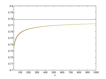
(a) under linear normalization

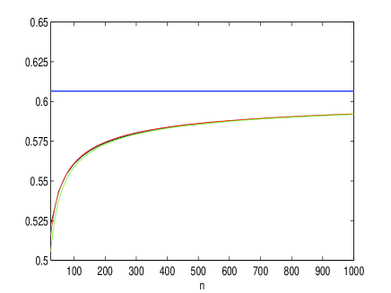
(b) under power normalization

Figure 1: Actual values and its approximations of the cdf of $M_{n}$ with $x=2$ under linear and power normalization, where the $\operatorname*{MSTD}$ is given by (4.1), and all asymptotics are given by (4.2). The actual values drawn in black, the first-order asymptotics drawn in blue, the second-order asymptotics drawn in red and the third-order asymptotics drawn in green.

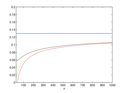
(a) under linear normalization

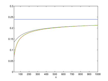
(b) under power normalization

Figure 2: Actual values and its approximations of the cdf of $M_{n}$ with $x=0.7$ under linear and power normalization, where the $\operatorname*{MSTD}$ is given by (4.1), and all asymptotics are given by (4.2). The actual values drawn in black, the first-order asymptotics drawn in blue, the second-order asymptotics drawn in red and the third-order asymptotics drawn in green.

In order to show the accuracy of all asymptotics more intuitive with varying $n$ , we then plot the actual values and its asymptotics of the cdf of $M_{n}$ with fixed $x$. With $x=2$, Figure 1 compares all asymptotics with the actual value under two different normalization; while Figure 2 shows the case of $x=0.7$. Tables 1-2 and Figures 1-2 show the following facts: i) For large $n$, the third-order asymptotics of the cdf of $M_{n}$ are closer to the actual values under the two different normalization. ii) For large $n$, $\Delta_{3}^{l}(2)$ is smaller than $\Delta_{3}^{p}(2)$, which shows that the third-order asymptotics of the cdf of $M_{n}$ at $x=2$ are more closer to its actual value under linear normalization. iii) For large $n$, $\Delta_{3}^{l}(0.7)$ is larger than $\Delta_{3}^{p}(0.7)$, which shows that the third-order asymptotic of the cdf of $M_{n}$ at $x=0.7$ are more closer to its actual value under power normalization.

Example 2. Let $X_{1}\sim\operatorname*{ST}_{3}(1)$, $X_{2}\sim\operatorname*{ST}_{6}(2)$, $X_{3}\sim\operatorname*{ST}_{8}(3)$, and $T^{\prime\prime}$ is defined by

$$T^{\prime\prime}=\left\{\begin{aligned} &X_{1},&\quad\operatorname*{P}(T^{\prime\prime}=X_{1})=0.5,&\\ &X_{2},&\quad\operatorname*{P}(T^{\prime\prime}=X_{2})=0.3,&\\ &X_{3},&\quad\operatorname*{P}(T^{\prime\prime}=X_{3})=0.2.&\\ \end{aligned}\right.$$ (4.3)

Let $M_{n}=\max_{1\leq k\leq n}\{T_{k}\}$ with $T_{k}\overset{d}{=}T^{\prime\prime}$, $k=1,\dots,n$. By using Theorem 3.2 (ii) and Remark 3.2, the asymptotics of the pdf of $M_{n}$ are given

$$\left\{\begin{aligned} &U_{1}^{l}(x)=\Phi_{3}^{{}^{\prime}}(x),\\ &U_{2}^{l}(x)=\left(1+\left(-\frac{3(4T_{4}(2)+2^{-1.5}C_{4})}{2T_{4}(2)}x^{-2}+\left(\frac{9C_{4}}{20\sqrt{2}T_{4}(2)}+3.6\right)x^{-5}\right)a_{n}^{-2}\right)\Phi_{3}^{{}^{\prime}}(x),\\ &U_{3}^{l}(x)=\left[1+\left(-\frac{3(4T_{4}(2)+2^{-1.5}C_{4})}{2T_{4}(2)}x^{-2}+\left(\frac{9C_{4}}{20\sqrt{2}T_{4}(2)}+3.6\right)x^{-5}\right)a_{n}^{-2}\right.\\ &\quad\quad\quad\quad\left.+\left((2x^{-3}-x^{-6})\frac{36\sqrt{6}C_{6}T_{7}(2\sqrt{7})}{5C_{3}T_{4}(2)}+\frac{\sqrt{3}}{\pi}T_{4}(2)(2-x^{-3})x^{-3}\right)a_{n}^{-3}\right]\Phi_{3}^{{}^{\prime}}(x),\\ &U_{i}^{p}(x)=\frac{x^{-\frac{2}{3}}}{3}U^{l}(x^{\frac{1}{3}}),\quad i=1,2,3.\end{aligned}\right.$$ (4.4)

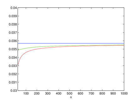
(a) under linear normalization

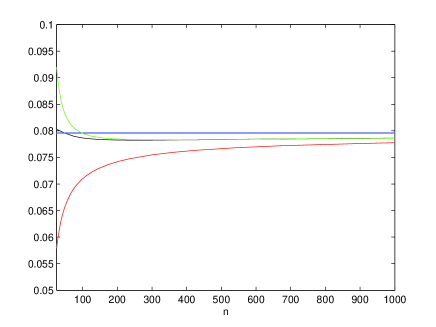
(b) under power normalization

Figure 3: Actual values and its approximations of the pdf of $M_{n}$ with $x=3$ under linear and power normalization, where the $\operatorname*{MSTD}$ is given by (4.3), and all asymptotics are given by (4.4). The actual values drawn in black, the first-order asymptotics drawn in blue, the second-order asymptotics drawn in red and the third-order asymptotics drawn in green.

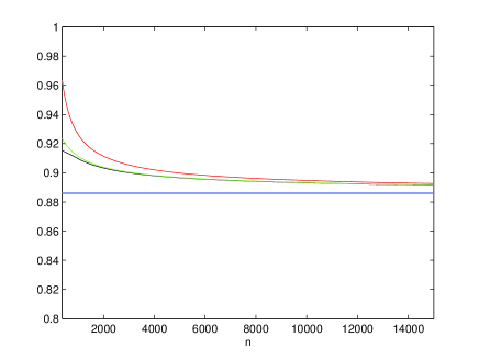
(a) under linear normalization

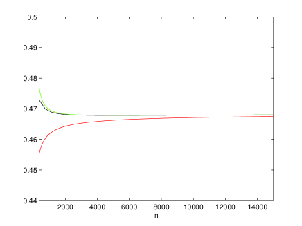
(b) under power normalization

Figure 4: Actual values and its approximations of the pdf of $M_{n}$ with $x=0.75$ under linear and power normalization, where the $\operatorname*{MSTD}$ is given by (4.3), and all asymptotics are given by (4.4). The actual values drawn in black, the first-order asymptotics drawn in blue, the second-order asymptotics drawn in red and the third-order asymptotics drawn in green.

Here, we calculate the absolute errors of the pdf of $M_{n}$ at $x=3$ for $n$ varying from $25$ to $1000$ with lattice $25$, and at $x=0.75$ for $n$ varying from $375$ to $15000$ with lattice $375$. Tables 3-4 document the numerical analysis results of $\delta_{i}^{l}(x)$ and $\delta_{i}^{p}(x)$, $i=1,2,3$, which show that the accuracy of all three kinds of asymptotics of pdf improve as $n$ becomes large. Figures 3-4 compare all asymptotics with the actual values under two different normalizations. From Tables 3-4 and Figures 3-4, we know that: i) For large $n$, the third-order asymptotics of pdf of $M_{n}$ are closer to the actual values under the two different normalization. ii) When $n$ is larger, $\delta_{3}^{l}(3)$ is smaller than $\delta_{3}^{p}(3)$, which shows that the third-order asymptotic of the pdf of $M_{n}$ at $x=3$ are more closer to its actual value under linear normalization. iii) For large $n$, $\delta_{3}^{l}(0.75)$ is larger than $\delta_{3}^{p}(0.75)$, which shows that the third-order asymptotic of the pdf of $M_{n}$ at $x=0.75$ are more closer to its actual value under power normalization.

Table 1: A̧bsolute errors between actual values and their asymptotics of the cdf at $x=2$

$n$	$\Delta_{1}^{l}(2)$	$\Delta_{1}^{p}(2)$	$\Delta_{2}^{l}(2)$	$\Delta_{2}^{p}(2)$	$\Delta_{3}^{l}(2)$	$\Delta_{3}^{p}(2)$
25	0.041618314	0.083694396	0.000428915	0.007036842	0.003937814	0.017246955
50	0.029959447	0.063092667	0.000834143	0.001064006	0.001349221	0.006169063
75	0.024516994	0.052450469	0.000736283	0.000066765	0.000719293	0.003336607
100	0.021225874	0.045767313	0.000631175	0.000401695	0.000460507	0.002150834
125	0.018967784	0.041089738	0.000547325	0.000513495	0.000326021	0.001528528
150	0.017297315	0.037586625	0.000481813	0.000545752	0.000245975	0.001155933
175	0.015998039	0.034839136	0.000429909	0.000545952	0.000193909	0.000912636
200	0.014950642	0.032610918	0.000387990	0.000532581	0.000157851	0.000743683
225	0.014083308	0.030757365	0.000353508	0.000513619	0.000131684	0.000620838
250	0.013349908	0.029184474	0.000324676	0.000492737	0.000111997	0.000528274
275	0.012719296	0.027828177	0.000300225	0.000471680	0.000096751	0.000456512
300	0.012169587	0.026643128	0.000279231	0.000451276	0.000084663	0.000399567
325	0.011684897	0.025596216	0.000261013	0.000431899	0.000074890	0.000353495
350	0.011253383	0.024662633	0.000245053	0.000413690	0.000066856	0.000315604
375	0.010866013	0.023823378	0.000230956	0.000396674	0.000060159	0.000284001
400	0.010515764	0.023063622	0.000218414	0.000380812	0.000054507	0.000257320
425	0.010197078	0.022371599	0.000207181	0.000366042	0.000049685	0.000234553
450	0.009905498	0.021737842	0.000197063	0.000352285	0.000045533	0.000214944
475	0.009637397	0.021154635	0.000187900	0.000339462	0.000041927	0.000197913
500	0.009389793	0.020615617	0.000179563	0.000327496	0.000038773	0.000183010
525	0.009160209	0.020115494	0.000171945	0.000316314	0.000035994	0.000169881
550	0.008946565	0.019649815	0.000164956	0.000305850	0.000033532	0.000158246
575	0.008747104	0.019214812	0.000158520	0.000296041	0.000031338	0.000147877
600	0.008560326	0.018807269	0.000152575	0.000286832	0.000029372	0.000138589
625	0.008384945	0.018424420	0.000147065	0.000278173	0.000027604	0.000130232
650	0.008219851	0.018063876	0.000141945	0.000270017	0.000026006	0.000122680
675	0.008064078	0.017723558	0.000137174	0.000262324	0.000024557	0.000115829
700	0.007916783	0.017401648	0.000132718	0.000255056	0.000023237	0.000109591
725	0.007777225	0.017096549	0.000128546	0.000248181	0.000022031	0.000103892
750	0.007644753	0.016806849	0.000124632	0.000241668	0.000020926	0.000098670
775	0.007518787	0.016531300	0.000120952	0.000235489	0.000019910	0.000093869
800	0.007398812	0.016268789	0.000117486	0.000229620	0.000018974	0.000089446
825	0.007284370	0.016018321	0.000114216	0.000224039	0.000018109	0.000085358
850	0.007175049	0.015779004	0.000111125	0.000218726	0.000017308	0.000081572
875	0.007070479	0.015550039	0.000108200	0.000213660	0.000016564	0.000078057
900	0.006970326	0.015330700	0.000105426	0.000208827	0.000015872	0.000074788
925	0.006874288	0.015120333	0.000102793	0.000204210	0.000015227	0.000071740
950	0.006782093	0.014918345	0.000100290	0.000199794	0.000014624	0.000068893
975	0.006693489	0.014724194	0.000097907	0.000195569	0.000014060	0.000066229
1000	0.006608252	0.014537388	0.000095636	0.000191520	0.000013532	0.000063733

Table 2: A̧bsolute errors between actual values and their asymptotics of the cdf at $x=0.7$

$n$	$\Delta_{1}^{l}(0.7)$	$\Delta_{1}^{p}(0.7)$	$\Delta_{2}^{l}(0.7)$	$\Delta_{2}^{p}(0.7)$	$\Delta_{3}^{l}(0.7)$	$\Delta_{3}^{p}(0.7)$
25	0.072769740	0.103763098	0.087495626	0.069370486	0.049301919	0.061652134
50	0.069353107	0.091767994	0.043971619	0.030655938	0.024874766	0.026796762
75	0.064006392	0.081576059	0.028522860	0.018382662	0.015791625	0.015809878
100	0.059391318	0.073922726	0.020741365	0.012644066	0.011192938	0.010714478
125	0.055557905	0.068015416	0.016114945	0.009412276	0.008476203	0.007868606
150	0.052351600	0.063304069	0.013076462	0.007377421	0.006710844	0.006091029
175	0.049632109	0.059441782	0.010942505	0.005996562	0.005486261	0.004893940
200	0.047292939	0.056204365	0.009369424	0.005007601	0.004595211	0.004042807
225	0.045255350	0.053441320	0.008166438	0.004269875	0.003922693	0.003412280
250	0.043460780	0.051047909	0.007219578	0.003701737	0.003400208	0.002929902
275	0.041865033	0.048948898	0.006456793	0.003252842	0.002984637	0.002551173
300	0.040434206	0.047088752	0.005830420	0.002890609	0.002647611	0.002247413
325	0.039141869	0.045425507	0.005307745	0.002593110	0.002369768	0.001999390
350	0.037967110	0.043926805	0.004865610	0.002345092	0.002137488	0.001793781
375	0.036893155	0.042567252	0.004487185	0.002135647	0.001940937	0.001621090
400	0.035906379	0.041326607	0.004159962	0.001956789	0.001772856	0.001474392
425	0.034995595	0.040188516	0.003874466	0.001802546	0.001627777	0.001348526
450	0.034151520	0.039139604	0.003623389	0.001668373	0.001501516	0.001239576
475	0.033366381	0.038168814	0.003401015	0.001550754	0.001390820	0.001144525
500	0.032633615	0.037266914	0.003202810	0.001446932	0.001293125	0.001061014
525	0.031947636	0.036426131	0.003025133	0.001354715	0.001206385	0.000987174
550	0.031303659	0.035639862	0.002865031	0.001272342	0.001128954	0.000921508
575	0.030697556	0.034902463	0.002720083	0.001198385	0.001059487	0.000862804
600	0.030125744	0.034209075	0.002588286	0.001131670	0.000996882	0.000810072
625	0.029585100	0.033555488	0.002467973	0.001071229	0.000940225	0.000762495
650	0.029072883	0.032938036	0.002357741	0.001016254	0.000888752	0.000719394
675	0.028586680	0.032353506	0.002256404	0.000966067	0.000841822	0.000680203
700	0.028124353	0.031799075	0.002162954	0.000920097	0.000798893	0.000644441
725	0.027684005	0.031272245	0.002076526	0.000877855	0.000759502	0.000611705
750	0.027263942	0.030770798	0.001996376	0.000838925	0.000723253	0.000581647
775	0.026862649	0.030292760	0.001921860	0.000802949	0.000689805	0.000553970
800	0.026478763	0.029836365	0.001852419	0.000769618	0.000658865	0.000528419
825	0.026111057	0.029400026	0.001787562	0.000738662	0.000630177	0.000504773
850	0.025758421	0.028982317	0.001726862	0.000709848	0.000603518	0.000482837
875	0.025419852	0.028581948	0.001669939	0.000682969	0.000578690	0.000462445
900	0.025094433	0.028197751	0.001616461	0.000657847	0.000555525	0.000443448
925	0.024781333	0.027828666	0.001566130	0.000634320	0.000533868	0.000425716
950	0.024479791	0.027473727	0.001518684	0.000612249	0.000513586	0.000409135
975	0.024189111	0.027132053	0.001473886	0.000591509	0.000494560	0.000393602
1000	0.023908653	0.026802837	0.001431526	0.000571986	0.000476683	0.000379028

Table 3: A̧bsolute errors between actual values and their asymptotics of the pdf at $x=3$

$n$	$\delta_{1}^{l}(3)$	$\delta_{1}^{p}(3)$	$\delta_{2}^{l}(3)$	$\delta_{2}^{p}(3)$	$\delta_{3}^{l}(3)$	$\delta_{3}^{p}(3)$
25	0.0008041273	0.0006725280	0.0019423949	0.0223613528	0.0000566926	0.0117149407
50	0.0007311965	0.0000831380	0.0009990041	0.0135799655	0.0000005396	0.0034581813
75	0.0006485578	0.0006433885	0.0006718323	0.0097835109	0.0000054698	0.0015752536
100	0.0005840952	0.0009576983	0.0005058628	0.0076495175	0.0000060910	0.0008695559
125	0.0005337537	0.0011375344	0.0004055436	0.0062799394	0.0000057262	0.0005353193
150	0.0004934233	0.0012425557	0.0003383704	0.0053259793	0.0000051892	0.0003534029
175	0.0004603054	0.0013037635	0.0002902528	0.0046232692	0.0000046689	0.0002447727
200	0.0004325366	0.0013381242	0.0002540939	0.0040840820	0.0000042080	0.0001754547
225	0.0004088465	0.0013554372	0.0002259309	0.0036572932	0.0000038100	0.0001289616
250	0.0003883432	0.0013616312	0.0002033771	0.0033110845	0.0000034683	0.0000965449
275	0.0003703823	0.0013604338	0.0001849095	0.0030246130	0.0000031743	0.0000732319
300	0.0003544865	0.0013542639	0.0001695107	0.0027836538	0.0000029201	0.0000560373
325	0.0003402938	0.0013447330	0.0001564749	0.0025781659	0.0000026989	0.0000430875
350	0.0003275248	0.0013329376	0.0001452973	0.0024008590	0.0000025053	0.0000331620
375	0.0003159599	0.0013196371	0.0001356072	0.0022463123	0.0000023347	0.0000254406
400	0.0003054237	0.0013053648	0.0001271265	0.0021104110	0.0000021835	0.0000193573
425	0.0002957744	0.0012904994	0.0001196421	0.0019899757	0.0000020488	0.0000145122
450	0.0002868962	0.0012753118	0.0001129885	0.0018825105	0.0000019281	0.0000106170
475	0.0002786930	0.0012599970	0.0001070346	0.0017860291	0.0000018194	0.0000074600
500	0.0002710848	0.0012446954	0.0001016756	0.0016989310	0.0000017212	0.0000048837
525	0.0002640041	0.0012295082	0.0000968267	0.0016199119	0.0000016320	0.0000027687
550	0.0002573936	0.0012145077	0.0000924184	0.0015478987	0.0000015508	0.0000010237
575	0.0002512043	0.0011997449	0.0000883933	0.0014820000	0.0000014764	0.0000004220
600	0.0002453940	0.0011852554	0.0000847035	0.0014214695	0.0000014082	0.0000016239
625	0.0002399263	0.0011710628	0.0000813089	0.0013656775	0.0000013454	0.0000026258
650	0.0002347692	0.0011571824	0.0000781755	0.0013140891	0.0000012875	0.0000034624
675	0.0002298950	0.0011436225	0.0000752741	0.0012662469	0.0000012338	0.0000041620
700	0.0002252792	0.0011303870	0.0000725800	0.0012217575	0.0000011840	0.0000047470
725	0.0002209002	0.0011174758	0.0000700718	0.0011802808	0.0000011377	0.0000052362
750	0.0002167386	0.0011048864	0.0000677308	0.0011415210	0.0000010946	0.0000056445
775	0.0002127775	0.0010926142	0.0000655409	0.0011052198	0.0000010542	0.0000059846
800	0.0002090015	0.0010806531	0.0000634880	0.0010711509	0.0000010165	0.0000062667
825	0.0002053970	0.0010689961	0.0000615595	0.0010391145	0.0000009811	0.0000064996
850	0.0002019515	0.0010576355	0.0000597445	0.0010089343	0.0000009478	0.0000066904
875	0.0001986540	0.0010465630	0.0000580333	0.0009804536	0.0000009166	0.0000068452
900	0.0001954943	0.0010357704	0.0000564173	0.0009535330	0.0000008871	0.0000069693
925	0.0001924633	0.0010252489	0.0000548886	0.0009280477	0.0000008592	0.0000070668
950	0.0001895527	0.0010149901	0.0000534405	0.0009038861	0.0000008329	0.0000071416
975	0.0001867548	0.0010049853	0.0000520667	0.0008809478	0.0000008080	0.0000071967
1000	0.0001840628	0.0009952262	0.0000507616	0.0008591422	0.0000007844	0.0000072349

Table 4: A̧bsolute errors between actual values and their asymptotics of the pdf at $x=0.75$

$n$	$\delta_{1}^{l}(0.75)$	$\delta_{1}^{p}(0.75)$	$\delta_{2}^{l}(0.75)$	$\delta_{2}^{p}(0.75)$	$\delta_{3}^{l}(0.75)$	$\delta_{3}^{p}(0.75)$
375	0.029225833	0.004206893	0.048225582	0.017429407	0.008274292	0.003965312
750	0.026010161	0.001357781	0.022781173	0.009687443	0.002805528	0.001009916
1125	0.022436305	0.000326059	0.014798452	0.006682780	0.001481355	0.000448792
1500	0.019788382	0.000153010	0.010948233	0.005094348	0.000960410	0.000254332
1875	0.017800136	0.000408380	0.008687875	0.004113656	0.000697617	0.000165288
2250	0.016254384	0.000555948	0.007202043	0.003448535	0.000543494	0.000117251
2625	0.015014707	0.000645367	0.006150896	0.002968027	0.000443569	0.000088361
3000	0.013994922	0.000700876	0.005367932	0.002604753	0.000374021	0.000069587
3375	0.013138561	0.000735459	0.004762043	0.002320534	0.000323010	0.000056657
3750	0.012407202	0.000756573	0.004279199	0.002092132	0.000284070	0.000047340
4125	0.011773795	0.000768735	0.003885333	0.001904593	0.000253397	0.000040382
4500	0.011218727	0.000774802	0.003557896	0.001747864	0.000228621	0.000035029
4875	0.010727415	0.000776643	0.003281370	0.001614938	0.000208194	0.000030810
5250	0.010288769	0.000775517	0.003044726	0.001500779	0.000191062	0.000027415
5625	0.009894201	0.000772289	0.002839907	0.001401679	0.000176487	0.000024636
6000	0.009536942	0.000767570	0.002660891	0.001314845	0.000163936	0.000022325
6375	0.009211582	0.000761796	0.002503088	0.001238134	0.000153013	0.000020379
6750	0.008913739	0.000755280	0.002362935	0.001169875	0.000143419	0.000018720
7125	0.008639821	0.000748254	0.002237626	0.001108745	0.000134926	0.000017293
7500	0.008386855	0.000740888	0.002124919	0.001053683	0.000127354	0.000016053
7875	0.008152358	0.000733310	0.002023003	0.001003829	0.000120561	0.000014967
8250	0.007934233	0.000725614	0.001930400	0.000958477	0.000114432	0.000014010
8625	0.007730701	0.000717871	0.001845886	0.000917045	0.000108874	0.000013160
9000	0.007540241	0.000710134	0.001768448	0.000879046	0.000103811	0.000012400
9375	0.007361541	0.000702444	0.001697231	0.000844070	0.000099180	0.000011719
9750	0.007193466	0.000694831	0.001631515	0.000811771	0.000094927	0.000011103
10125	0.007035027	0.000687317	0.001570686	0.000781852	0.000091009	0.000010545
10500	0.006885357	0.000679917	0.001514218	0.000754059	0.000087387	0.000010038
10875	0.006743695	0.000672644	0.001461660	0.000728175	0.000084029	0.000009574
11250	0.006609368	0.000665505	0.001412617	0.000704009	0.000080907	0.000009148
11625	0.006481779	0.000658506	0.001366749	0.000681396	0.000077998	0.000008757
12000	0.006360395	0.000651650	0.001323758	0.000660190	0.000075280	0.000008395
12375	0.006244742	0.000644938	0.001283381	0.000640264	0.000072736	0.000008061
12750	0.006134393	0.000638371	0.001245387	0.000621506	0.000070349	0.000007750
13125	0.006028964	0.000631947	0.001209571	0.000603816	0.000068105	0.000007462
13500	0.005928109	0.000625666	0.001175750	0.000587105	0.000065992	0.000007192
13875	0.005831515	0.000619525	0.001143764	0.000571295	0.000063999	0.000006941
14250	0.005738896	0.000613522	0.001113466	0.000556314	0.000062116	0.000006705
14625	0.005649995	0.000607653	0.001084726	0.000542099	0.000060334	0.000006484
15000	0.005564575	0.000601917	0.001057428	0.000528592	0.000058646	0.000006276

Acknowledgements  This work was supported by the National Natural Science Foundation of China Grant No. 11171275, and the Doctoral Grant of University of Shanghai for Science and Technology (BSQD201608).

References

- [1] Azzalini, A. and Capitanio, A. (2003). Distributions generated by perturbation of symmetry with emphasis on a multivariate skew t distribution. Journal of the Royal Statistical Society: Series B, 65, 367–389.
- [2] Cabral C. R. B., Bolfarine, H. and Pereira, J. R. G. (2008). Bayesian density estimation using skew student-t-normal mixtures. Computational Statistics and Data Analysis, 52(12), 5075–5090.
- [3] Dellaportas, P. and Papageorgiou, I. (2006). Multivariate mixtures of Normals with unknown number of components. Statistics and Computing, 16(1), 57–68.
- [4] Frigessi, A. and Haug, O. and Rue, H. (2002). A dynamic mixture model for unsupervised tail estimation without threshold selection. Extremes, 5, 219–235.
- [5] Frühwirth-Schnatter, S. and Pyne, S. (2010). Bayesian inference for finite mixtures of univariate and multivariate skew-normal and skew-t distributions. Biostatistics, 11(2), 317–336.
- [6] Ho, H. J. and Lin, T. I. (2010). Robust linear mixed models using the skew t distribution with application to schizophrenia data. Biometrical Journal, 52(4), 449–469.
- [7] Lee, S. X. and McLachlan, G. J. (2013). On mixtures of skew normal and skew t distributions. Advances in Data Analysis and Classification, 7(3), 241–266.
- [8] Lee, S. and McLachlan, G. J. (2014). Finite mixtures of multivariate skew t-distributions: some recent and new results. Statistics and Computing, 24(2), 181–202.
- [9] Lin, T. I. (2010). Robust mixture modeling using multivariate skew t distribution. Statistics and Computing, 20(3), 343–356.
- [10] Lin, T. I., Lee, J. C. and Hsieh, W. J. (2007). Robust mixture modeling using the skew t distribution. Statistics and Computing, 17, 81–92.
- [11] Mohan, N. R. and Ravi, S. (1993). Max domains of attraction of univariate and multivariate -max stable laws. Theory of Probability and Its Applications, 37, 632–643.
- [12] Peng, Z., Li, C. and Nadarajah, S. (2016). Extremal properties of the skew-t distribution. Statistics and Probability Letters, 112, 10–19.
- [13] Resnick, S. I. Extreme Values, Regular Variation, and Point Processes. Springer Verlag, New York, 1987.
- [14] Pantcheva, E. (1985). Limit theorems for extreme order statistics under nonlinear normalization. In Stability problems for stochastic models, pp. 284–309. Springer Berlin Heidelberg.
- [15] Peel, D. and Mclachlan, G. J. (2000). Robust mixture modelling using the t distribution. Statistics and Computing, 10, 339–348
- [16] Sattayatham, P. and Talangtam, T. (2012). Fitting of finite mixture distributions to motor insurance claims. Journal of Mathematics and Statistics, 8, 49–56.
- [17] Vrbik, I. and McNicholas, (2012). Analytic calculations for the EM algorithm for multivariate skew-t mixture models. Statistics and Probability Letters, 82, 1169–1174.
- [18] Zou, Y. and Zhang, T. (2011). Use of skew-normal and skew-t distributions for mixture modeling of freeway speed data. Transportation Research Record: Journal of the Transportation Research Board, 2260, 67–75.