Extended Gauss-Newton and ADMM-Gauss-Newton algorithms for low-rank matrix optimization

Abstract. In this paper, we develop a variant of the well-known Gauss-Newton (GN) method to solve a class of nonconvex optimization problems involving low-rank matrix variables. As opposed to standard GN method, our algorithm allows one to handle general smooth convex objective function. We show, under mild conditions, that the proposed algorithm globally and locally converges to a stationary point of the original problem. We also show empirically that the GN algorithm achieves higher accurate solutions than the alternating minimization algorithm (AMA). Then, we specify our GN scheme to handle the symmetric case and prove its convergence, where AMA is not applicable. Next, we incorporate our GN scheme into the alternating direction method of multipliers (ADMM) to develop an ADMM-GN algorithm. We prove that, under mild conditions and a proper choice of the penalty parameter, our ADMM-GN globally converges to a stationary point of the original problem. Finally, we provide several numerical experiments to illustrate the proposed algorithms. Our results show that the new algorithms have encouraging performance compared to existing methods.

Keywords. Low-rank approximation, Gauss-Newton method, nonconvex alternating direction method of multipliers, quadratic and linear convergence.

1. Introduction

Problem statement:

In this paper, we consider the following class of low-rank matrix nonconvex optimization problems:

$$\Phi^{\star}:=\min_{U,V}\Big{\{}\Phi(U,V):=\phi\left(\mathcal{A}(UV^{\top})-B\right)+\mathcal{R}(U,V)\ :\ U\in\mathbb{R}^{m\times r},\ V\in\mathbb{R}^{n\times r}\Big{\}},$$ (1.1)

where $\mathcal{A}(Z):=[\mathrm{trace}\left(A_{1}^{\top}Z\right),\mathrm{trace}\left(A_{2}^{\top}Z\right),\cdots,\mathrm{trace}\left(A_{l}^{\top}Z\right)]$ for $l$ matrices $A_{1},\cdots,A_{l}$ in $\mathbb{R}^{m\times n}$ is a linear operator; $\phi:\mathbb{R}^{l}\to\mathbb{R}\cup\{+\infty\}$ is a proper, closed and convex function; and $B\in\mathbb{R}^{l}$ is an observed vector. The function $\mathcal{R}$ is often referred to as a regularizer, which can be chosen as $\mathcal{R}(U,V):=\frac{1}{4}\|U^{\top}U-V^{\top}V\|_{F}^{2}$ as suggested in [41]. Clearly, (1.1) is nonconvex due to the bilinear term $UV^{\top}$. Hence, it is NP-hard [33], and numerical methods for solving (1.1) aim at obtaining a local optimum or a stationary point of (1.1). In this paper, we are interested in the low-rank case, where $r\ll\min\left\{m,n\right\}$.

Problem (1.1) covers various practical models in low-rank embedded problems, function learning, matrix completion in recommender systems, inpainting and compression in image processing, robust principal component analysis in statistics, and semidefinite programming relaxations in combinatorial optimization, see, e.g., [10, 12, 15, 17, 29, 32, 44]. Among these applications, the following problems have been recently attracted a great attention. The most common case is when $\phi(\cdot):=(1/2)\|\cdot\|_{2}^{2}$, where (1.1) becomes a least-squares low-rank approximation problem in compressive sensing (see, e.g., [29]):

$$\min_{U,V}\big{\{}(1/2)\|\mathcal{A}(UV^{\top})-B\|_{2}^{2}\ :\ U\in\mathbb{R}^{m\times r},\ V\in\mathbb{R}^{n\times r}\big{\}}.$$ (1.2)

Here, the linear operator $\mathcal{A}$ is often assumed to satisfy a restricted isometric property (RIP) [11] that allows us to recover an exact solution from a few number of observations in $B$. In particular, if $\mathcal{A}=\mathcal{P}_{\Omega}$, the projection on a given index subset $\Omega$, then (1.2) covers the matrix completion model:

$$\min_{U,V}\big{\{}(1/2)\|\mathcal{P}_{\Omega}(UV^{\top})-B_{\Omega}\|_{F}^{2}\ :\ U\in\mathbb{R}^{m\times r},\ V\in\mathbb{R}^{n\times r}\big{\}},$$ (1.3)

where $B_{\Omega}$ is the observed entries in $\Omega$. If $\mathcal{A}$ is an identity operator and $B\in\mathbb{R}^{m\times n}$ is a given, then (1.2) becomes a low-rank matrix factorization problem

$$\Phi^{\star}:=\min_{U,V}\big{\{}\Phi(U,V)=(1/2)\|UV^{\top}-B\|^{2}_{F}~{}:~{}U\in\mathbb{R}^{m\times r},~{}V\in\mathbb{R}^{n\times r}\big{\}}.$$ (1.4)

Especially, if $U=V$ and $B$ is symmetric positive definite, then (1.4) reduces to

$$\Phi^{\star}:=\min_{U}\big{\{}\Phi(U):=(1/2)\|UU^{\top}-B\|_{F}^{2}\ :\ U\in\mathbb{R}^{n\times r}\big{\}},$$ (1.5)

which is studied in [32]. Alternatively, if we choose $\Phi(U):=(1/2)\|\mathcal{A}(UU^{\top})-B\|_{F}^{2}$ in (1.2), then (1.1) reduces to the case investigated in [3]. While both special cases, (1.4) and (1.5), possess a closed form solution via a truncated SVD and an eigenvalue decomposition, respectively, GN methods can also be applied to solve these problems. In [32], the authors demonstrated the advantages of a GN method for solving (1.5) with significantly encouraging performance.

Related work:

The low-rank structure is key to recast many existing problems into new frameworks or to design new models by means of regularizers to promote solution structures in various applications such as matrix completion (MC) [10], robust principal component analysis (RPCA) [13], and their variants. Hitherto, extensions to group structured sparsity, low-rankness, tree models, and tensor representation have attracted a great attention in recent years, see, e.g., [16, 21, 24, 28, 37, 39, 46]. A majority of research for low-rank models focuses on estimating sample complexity results for specific instances of (1.1), while numerous recent papers revolve around the RPCA settings, MC, and their extensions [13, 10, 26].

Along with modeling, solution methods have also been extensively developed for solving concrete instances of (1.1) in low-rank matrix completion and recovery settings. Among various approaches, convex optimization is perhaps one of the most powerful tools to solve several instances of (1.1), including MC, RPCA, their variants, and extensions. Unfortunately, convex models only provide an approximation to the low-rank model (1.1) by convex relaxations using, e.g., nuclear or max norms, which may not adequately approximate the desired rank. Alternatively, nonconvex as well as discrete optimization methods have also been considered for solving (1.1), see, e.g., [7, 29, 31, 38, 44, 45]. While these approaches work directly on the original problem (1.1), they can only find a local optimum or a critical point, and strongly depend on the priori knowledge of problems, the initial points of algorithm, and predicted ranks. However, recent empirical evidence has been provided to support these approaches, and surprisingly, in many cases, they outperform the convex optimization approach in terms of “accuracy” to the original model, and the overall computational time [29, 31, 44]. Other approaches such as stochastic gradient descent, Riemann manifold descent, greedy methods, parallel and distributed algorithms have also recently been studied for solving (1.1), see, e.g., [5, 26, 27, 42, 45].

Motivation:

Gauss-Newton (GN) methods work extremely well for nonlinear least-squares problems [4]. When $\phi$ is quadratic and the residual term $\mathcal{A}(UV^{\top})-B$ in (1.1) is small or zero at solutions, they can achieve local superlinear and even quadratic convergence rate. With a “good” initial point (i.e., close to the set of stationary points), GN methods often reach a stationary point within a few iterations [14]. Such a “good” initial point can be obtained using priori knowledge of the problem and the underlying algorithm (e.g., steady states of dynamical systems, or previous iterations of the algorithm) as a warm-start strategy.

As in classical GN methods, we develop an iterative scheme for solving (1.1) by using a linearization of $\mathcal{A}(UV^{\top})-B$ and a quadratic surrogate of $\phi$. At each iteration, it requires to solve a simple convex problem to form a GN direction and then incorporates with a globalization strategy to update the next iteration. In our setting, computing GN direction reduces to solving a linear least-squares problem. Comparing to the alternating minimization method (AMA) [44] that alternatively solves for each $U$ and $V$, GN simultaneously solves for $U$ and $V$ using the linearization of $UV^{\top}$. We have observed that (cf Subsection 6.2) GN uses a linearization of $UV^{\top}$ providing a good local approximate model to $UV^{\top}$ compared to the alternating form $U\bar{V}^{\top}$ (or $\bar{U}V^{\top}$), when $U-\bar{U}$ (or $V-\bar{V})$ is relatively large. This makes AMA saturated and does not significantly improve the objective values. In addition, without regularization, AMA may fail to converge as indicated by a counterexample in [20]. Moreover, AMA is not applicable to solving the symmetric case of (1.1) as shown in Section 5, but the GN method is.

While GN methods often use in nonlinear least squares [35], they have not widely been exploited for matrix optimization. Our aim in this paper is to extend the GN method for solving a class of problems (1.1) with a general smooth convex objective function $\phi$ and low-rank matrix variables. This paper is also inspired by a recent work [32], where the authors proposed a simple symmetric GN scheme to solve (1.5), and demonstrated its very encouraging performance.

Contribution:

Our contribution in this paper can be summarized as follows:

• We extend the GN method to solve the low-rank matrix optimization problem (1.1) with smooth convex objective function $\phi$. We prove the existence of a GN direction and provide a closed form formulation to compute it. We empirically show that our GN method can achieve higher accurate solutions than the well-known AMA scheme within the same number of iterations in certain cases.

• We show that there exists an explicit step-size to guarantee a descent property of the GN direction, which allows us to perform a backtracking linesearch procedure. We specify our framework to the symmetric case. Under mild conditions, we prove a global convergence of the proposed methods.

• We prove a local linear and quadratic convergence rate of the full-step GN variant under standard assumptions imposed on (1.1) at its solution set.

• We also combine an alternating direction method of multipliers (ADMM) and the GN method to obtain a new algorithm for handling (1.1). Under standard assumptions on (1.1), we prove global convergence of the proposed algorithm.

Unlike AMA whose only achieves a sublinear convergence even with good initial points, GN methods may require additional computation for GN directions, but they can achieve a fast local linear or quadratic convergence rate, which is key for online and real-time implementations by using warm-start. Alternatively, gradient descent-based methods can achieve local linear convergence but often require much strong assumptions imposed on (1.1). In contrast, GN methods work with the “small residual” setting under mild assumptions, and can easily achieve high accuracy solutions within a small number of iterations.

Paper outline:

The rest of this paper is organized as follows. We first review basic concepts related to problem (1.1) in Section 2. Section 3 presents a linesearch GN method for solving (1.1) and its convergence guarantees. Section 4 develops an ADMM-Gauss-Newton algorithm to solve (1.1) and investigates its global convergence. Section 5 specifies the GN algorithm to the symmetric case and proves its convergence. Section 6.1 discusses the implementation aspects of our algorithms and their extension to the nonsmooth objective function case. Numerical experiments are conducted in Section 6 with several examples in different fields. For the sake of presentation, we move all the proofs in the main text to the appendix.

2. Basic notation and optimality condition

We briefly describe basic notation, the optimality condition of (1.1), and our assumptions.

2.1. Basic notation and concepts

For a matrix $X$, $\sigma_{\min}(X)$ and $\sigma_{\max}(X)$ denote its positive smallest and largest singular values, respectively. If $X$ is symmetric, then $\lambda_{\min}(X)$ and $\lambda_{\max}(X)$ denote its smallest and largest eigenvalues, respectively. We use $X=P\Sigma Q^{\top}$ for SVD and $X=U\Lambda U^{-1}$ for eigenvalue decomposition. $X^{\dagger}$ denotes the Moore-Penrose pseudo-inverse of $X$. When $X$ is full-column rank, $X^{\dagger}=(X^{\top}X)^{-1}X^{\top}$. We define $P_{X}:=XX^{\dagger}$ the projection onto the range space of $X$, and $P_{X}^{\perp}:=\mathbb{I}-P_{X}$ the orthogonal projection of $P_{X}$, i.e., $P_{X}P^{\perp}_{X}=P_{X}^{\perp}P_{X}=0$, where $\mathbb{I}$ is the identity matrix. Clearly, $P_{X}^{\perp}X=0$. We define $\mathrm{vec}\left(X\right)=(X_{11},\cdots X_{m1},\cdots,X_{1n},\cdots,X_{mn})^{\top}$ the vectorization of $X$, and $\mathrm{mat}$ the inverse mapping of $\mathrm{vec}$, i.e., $\mathrm{mat}\left(\mathrm{vec}\left(X\right)\right)=X$. $X\otimes Y$ denotes the Kronecker product of $X$ and $Y$. We have $\mathrm{vec}\left(AXB\right)=(B^{\top}\otimes A)\mathrm{vec}\left(X\right)$ and $(A\otimes B)(C\otimes D)=AC\otimes BD$. $\mathcal{A}^{*}$ denotes the adjoint of a linear operator $\mathcal{A}$. We say that a continuously differentiable function $f$ is $L_{f}$-smooth if there exists a constant $L_{f}\in[0,+\infty)$ such that $\|\nabla{f}(x)-\nabla{f}(y)\|_{2}\leq L_{f}\|x-y\|_{2}$ for all $x,y\in\mathrm{dom}(f)$. Here, $L_{f}$ is called a Lipschitz constant of $f$. A function $f$ is said to be $\mu_{f}$-strongly convex if $f(\cdot)-\frac{\mu_{f}}{2}\left\|\cdot\right\|^{2}_{2}$ remains convex. If $\mu_{f}=0$, then $f$ is just convex.

2.2. Optimality condition and basic assumptions

We define $X:=[U,V]$ as the joint variable of $U$ and $V$. We assume that $\phi$ in (1.1) is smooth. The optimality condition of (1.1) can be written as follows:

$$\left\{\begin{array}[]{ll}U_{\star}^{\top}\mathcal{A}^{*}\left(\nabla{\phi}(\mathcal{A}(U_{\star}V_{\star}^{\top})-B)\right)&=0,\vspace{0.75ex}\\ \mathcal{A}^{*}\left(\nabla{\phi}(\mathcal{A}(U_{\star}V_{\star}^{\top})-B)\right)V_{\star}&=0.\end{array}\right.$$ (2.1)

Any $X_{\star}=[U_{\star},V_{\star}]$ satisfying (2.1) is called a stationary point of (1.1). We denote by $\mathcal{X}_{\star}$ the set of stationary points of (1.1). Since $r\leq\min\left\{m,n\right\}$, the solution of (2.1) is generally nonunique. Our aim is to design algorithms for generating a sequence $\left\{X_{k}\right\}$ converging to $X_{\star}\in\mathcal{X}_{\star}$ under the following assumptions.

Assumption 2.1.

Problem (1.1) satisfies the following conditions:

• The set $\mathcal{X}_{\star}$ of stationary points of (1.1) is nonempty, and $\Phi^{\star}>-\infty$ in (1.1).

• $\phi$ is $L_{\phi}$-smooth and $\mu_{\phi}$-convex with $0\leq\mu_{\phi}\leq L_{\phi}<+\infty$.

We allow $\mu_{\phi}=0$, which also covers the non-strongly convex case. Since $\phi$ is smooth and $\mathcal{A}$ is linear, $\Phi$ in (1.1) is also smooth. Moreover, as shown in [34], $\phi$ satisfies

$$\frac{\mu_{\phi}}{2}\left\|y-x\right\|_{2}^{2}\leq\phi(y)-\phi(x)-\langle\nabla{\phi}(x),y-x\rangle\leq\frac{L_{\phi}}{2}\|y-x\|_{2}^{2},\quad\forall x,y\in\mathrm{dom}(\phi).$$ (2.2)

Note that Assumption A.2.1(b) covers a wide range of applications, including logistic loss, Huber loss, and entropy function in statistics and machine learning [6].

3. Linesearch Gauss-Newton method

In this section, we develop a linesearch Gauss-Newton (Ls-GN) algorithm for solving (1.1).

3.1. Forming a surrogate of the objective

By Assumption A.2.1, it follows from (2.2) and $\Phi(U,V):=\phi(\mathcal{A}(UV^{\top})-B)$ that

$$\Phi(\hat{U},\hat{V})\leq\Phi(U,V)+\frac{L_{\Phi}}{2}\|\hat{U}\hat{V}^{\top}-(UV^{\top}-L_{\Phi}^{-1}\Phi^{\prime}(UV^{\top}))\|_{F}^{2}-\frac{1}{2L_{\Phi}}\|\Phi^{\prime}(UV^{\top})\|_{F}^{2},$$ (3.1)

for any $U$, $V$, $\hat{U}$, and $\hat{V}$, where $\Phi^{\prime}(UV^{\top}):=\mathcal{A}^{*}\nabla{\phi}(\mathcal{A}(UV^{\top})-B)$, and $L_{\Phi}:=L_{\phi}\|\mathcal{A}\|^{2}$ is the Lipschitz constant of the gradient of $\phi(\mathcal{A}(\cdot)-B)$.

Gradient descent-type methods rely on finding a descent direction of $\Phi$ by approximately minimizing the right-hand side surrogate of $\Phi$ in (3.1). Unfortunately, this surrogate remains nonconvex due to the bilinear term $\hat{U}\hat{V}^{\top}$. Our next step is to linearize this term around a given point $[U,V]$ as follows:

$$\hat{U}\hat{V}^{\top}\approx UV^{\top}+U(\hat{V}-V)^{\top}+(\hat{U}-U)V^{\top}.$$ (3.2)

Then, the minimization of the right-hand side of (3.1) is approximated by

$$\min_{\hat{U},\hat{V}}\left\{(1/2)\|U(\hat{V}-V)^{\top}+(\hat{U}-U)V^{\top}+L_{\Phi}^{-1}\Phi^{\prime}(UV^{\top})\|_{F}^{2}\right\}.$$ (3.3)

This is a linear least-squares problem, and can be solved by standard linear algebra routines.

3.2. Computing Gauss-Newton direction

Let us define

$$D_{U}:=\hat{U}-U,\quad D_{V}:=\hat{V}-V,\quad\text{and}\quad Z:=-L_{\Phi}^{-1}\mathcal{A}^{\ast}\left(\nabla{\phi}(\mathcal{A}(UV^{\top})-B)\right).$$

Then, we rewrite (3.3) as

$$\min_{D_{U},D_{V}}\left\{(1/2)\|UD_{V}^{\top}+D_{U}V^{\top}-Z\|_{F}^{2}\ :\ D_{U}\in\mathbb{R}^{m\times r},D_{V}\in\mathbb{R}^{m\times r}\right\}.$$ (3.4)

The optimality condition of (3.4) becomes

$$\left\{\begin{array}[]{llcl}&U^{\top}UD_{V}^{\top}+U^{\top}D_{U}V^{\top}&=&U^{\top}Z,\vspace{1ex}\\ &UD_{V}^{\top}V+D_{U}V^{\top}V&=&ZV.\end{array}\right.$$ (3.5)

As usual, we refer to (3.5) as the normal equation of (3.4). We will construct a closed form solution of (3.5) in Lemma 3.1, whose proof is in Appendix A.1.

Lemma 3.1.

The rank of the square linear system (3.5) does not exceed $r(m+n-r)$. In addition, (3.5) has a solution. If $\mathrm{rank}\left(U\right)=\mathrm{rank}\left(V\right)=r\leq\min\left\{m,n\right\}$, then the solution of (3.5) is given explicitly by

$$\left\{\begin{array}[]{lcl}D_{U}&=&P^{\perp}_{U}Z(V^{\dagger})^{\top}+U\hat{D}_{r},\vspace{1ex}\\ D_{V}^{\top}&=&U^{\dagger}Z-\hat{D}_{r}V^{\top},\end{array}\right.$$ (3.6)

which forms a linear subspace in $\mathbb{R}^{r\times r}$, and $\hat{D}_{r}\in\mathbb{R}^{r\times r}$ is an arbitrary matrix.

In particular, if we choose $\hat{D}_{r}:=0.5U^{\dagger}Z(V^{\dagger})^{\top}\in\mathbb{R}^{r\times r}$, then

$$D_{U}=\big{(}\mathbb{I}_{m}-0.5P_{U}\big{)}Z(V^{\dagger})^{\top}\quad\text{and}\quad D_{V}^{\top}=U^{\dagger}Z\big{(}\mathbb{I}_{n}-0.5P_{V}\big{)}.$$ (3.7)

Moreover, the optimal value of (3.4) is $(1/2)\|P^{\perp}_{U}ZP^{\perp}_{V}\|_{F}^{2}$.

Lemma 3.1 also shows that if either $Z$ is in the null space of $P_{U}$ or $Z^{\top}$ is in the null space of $P_{V}$, then $\|P^{\perp}_{U}ZP^{\perp}_{V}\|_{F}^{2}=0$. Since (3.7) only gives us one choice for $D_{X}:=[D_{U},D_{V}]$, if $\hat{D}_{r}=\boldsymbol{0}^{r}$, we obtain another simple GN search direction.

Remark 3.1.

Let $m=n$. If we assume that $U=V$, then $D_{U}=D_{V}$ and

$$D_{U}=P^{\perp}_{U}Z(U^{\dagger})^{\top}+U\hat{D}_{r},\quad\text{where}\quad\hat{D}_{r}\in\mathcal{S}_{r}:=\left\{\hat{D}_{r}\in\mathbb{R}^{r\times r}\ :\ \hat{D}_{r}+\hat{D}_{r}^{\top}=U^{\dagger}Z(U^{\dagger})^{\top}\right\}.$$

Clearly, $\mathcal{S}_{r}$ is a linear subspace, and its dimension is $r(r+1)/2$.

3.3. The damped-step Gauss-Newton scheme

Using Lemma 3.1, we can form a damped step GN scheme as follows:

$$\left\{\begin{array}[]{lcl}U_{+}&:=&U+\alpha D_{U},\vspace{1ex}\\ V_{+}&:=&V+\alpha D_{V},\end{array}\right.$$ (3.8)

where $D_{U}$ and $D_{V}$ defined in (3.7) is a GN direction, and $\alpha>0$ is a given step-size determined in the next lemma.

Since the GN direction computed from (3.4) is not unique, we need to choose an appropriate $D_{X}$ such that it is a descent direction of $\Phi$ at $X$. We prove in Lemma 3.2 that (3.7) indeed gives a descent direction of $\Phi$ at $X$. The proof of this lemma is deferred to Appendix A.2.

Lemma 3.2.

Let $X:=[U,V]$ be a non-stationary point of (1.1) and $D_{X}:=[D_{U},D_{V}]$ be given by (3.7). If $D_{X}\neq 0$ and $\alpha$ is chosen in $0<\alpha\leq\underline{\alpha}$ where

$$\underline{\alpha}:=\min\left\{1,\frac{L_{\Phi}\sigma_{\min}^{3}}{2\|\nabla{\Phi}(U,V)\|_{F}},\frac{3\sigma_{\min}^{4}}{32\sigma_{\max}^{2}\|\Phi^{\prime}(UV^{\top})\|_{F}}\right\}\in(0,1],$$ (3.9)

then we have

$$\Phi(U_{+},V_{+})\leq\Phi(U,V)-\frac{\alpha\sigma_{\min}^{2}}{128L_{\Phi}\sigma_{\max}^{4}}\|\nabla{\Phi}(U,V)\|^{2},$$ (3.10)

where $\Phi^{\prime}(\cdot)=\mathcal{A}^{*}\nabla{\phi}(\mathcal{A}(\cdot)-B)$, $L_{\Phi}:=L_{\phi}\left\|\mathcal{A}\right\|^{2}$, $\sigma_{\min}:=\min\left\{\sigma_{\min}(U),\sigma_{\min}(V)\right\}$, and $\sigma_{\max}:=\max\left\{\sigma_{\max}(U),\sigma_{\max}(V)\right\}$. Hence, $D_{X}$ is a descent direction of $\Phi$.

Lemma 3.2 shows that if the residual term $\mathcal{A}^{*}\nabla{\phi}(\mathcal{A}(UV^{\top})-B)$ is sufficient small near $\mathcal{X}_{\star}$, then we obtain a full-step size $\alpha=1$.

The existence of the GN direction in Lemma 3.1 requires $U$ and $V$ to be full-rank. We prove in Appendix A.3 the following lemma.

Lemma 3.3.

If $\mathrm{rank}\left(U\right)=\mathrm{rank}\left(V\right)=r$, then $X_{+}:=[U_{+},V_{+}]$ updated by (3.8) using the step-size $\underline{\alpha}$ in (3.9) satisfies

$$\sigma_{\min}(U_{+})\geq 0.5\sigma_{\min}(U)\quad\text{and}\quad\sigma_{\min}(V_{+})\geq 0.5\sigma_{\min}(V).$$ (3.11)

Hence, (3.8) preserves the rank of $U_{+}$ and $V_{+}$, i.e., $\mathrm{rank}\left(U_{+}\right)=\mathrm{rank}\left(V_{+}\right)=r$.

3.4. The algorithmic template and its global convergence

Theoretically, we can use the step-size $\underline{\alpha}$ in Lemma 3.2 for (3.8). However, in practice, computing $\underline{\alpha}$ requires a high computational cost. We instead incorporate the GN scheme (3.8) with an Armijo backtracking linesearch to find an appropriate step-size $\alpha\geq\beta\underline{\alpha}$ for a given $\beta\in(0,1)$.

Find the smallest integer number $i_{k}\geq 0$ such that $\alpha:=\beta^{i_{k}}\alpha_{0}\geq\underline{\alpha}$ and

$$\Phi(U+\alpha D_{U},V+\alpha D_{V})\leq\Phi(U,V)-0.5c_{1}\alpha\|\nabla{\Phi}(U,V)\|_{F}^{2},$$ (3.12)

where $\alpha_{0}>0$, $c_{1}>0$, and $\beta\in(0,1)$ are given (e.g., $c_{1}:=0.5$ and $\beta:=\frac{\sqrt{5}-1}{\sqrt{5}+1}$).

By Lemma 3.2, this procedure is terminated after a finite number of iterations $i_{k}$ such that

$$0\leq i_{k}\leq\lfloor\log_{\beta}(\underline{\alpha}/\alpha_{0})\rfloor+1,$$ (3.13)

where $\underline{\alpha}$ is given by (3.9). Now, we describe the complete linesearch GN algorithm for approximating a stationary point of (1.1) as in Algorithm 1.

Algorithm 1 (Linesearch Gauss-Newton Algorithm (Ls-GN))

1:  Initialization: Given a tolerance $\varepsilon>0$. Choose $X_{0}:=[U_{0},V_{0}]$. Set $c_{1}:=0.5$ and $\alpha_{0}:=1$.

2:  for $k=0$ to $k_{\max}$ do

3:      GN direction: Let $Z_{k}:=-L_{\Phi}^{-1}\Phi^{\prime}(U_{k}V_{k}^{\top})$. Compute $D_{X_{k}}:=[D_{U_{k}},D_{V_{k}}]$:

$$D_{U_{k}}:=\left(\mathbb{I}_{m}-0.5P_{U_{k}}\right)Z_{k}(V_{k}^{\dagger})^{\top}\quad\text{and}\quad D_{V_{k}}=\left(\mathbb{I}_{n}-0.5P_{V_{k}}\right)Z_{k}^{\top}(U_{k}^{\dagger})^{\top}.\vspace{-2ex}$$

4:     Stopping criterion: If stopping_criterion, then TERMINATE.

5:      Backtracking linesearch: Find the smallest integer number $i_{k}\geq 0$ such that

$$\Phi(U_{k}+\alpha_{k}D_{U_{k}},V_{k}+\alpha_{k}D_{V_{k}})\leq\Phi(U_{k},V_{k})-0.5c_{1}\alpha_{k}\|\nabla{\Phi}(U_{k},V_{k})\|_{F}^{2},$$

where $\alpha_{k}:=\alpha_{0}\beta^{i_{k}}$.

6:     Update $X_{k+1}:=[U_{k+1},V_{k+1}]$ as $U_{k+1}:=U_{k}+\alpha_{k}D_{U_{k}}$ and $V_{k+1}:=V_{k}+\alpha_{k}D_{V_{k}}$.

7:  end for

Per-teration complexity:

The main steps of Algorithm 1 are Steps 3 and 5, i.e. computing $D_{X_{k}}$ and performing the linesearch routine, respectively.

• Computing $D_{X_{k}}$ requires two inverses $(U^{\top}U)^{-1}$ and $(V^{\top}V)^{-1}$ of the size $r\times r$, and two matrix-matrix multiplications (of the size $m\times r$ or $n\times r$).

• Evaluating $\Phi^{\prime}$ requires one matrix-matrix multiplication $UV^{\top}$ and one evaluation of the form $\mathcal{A}^{*}\nabla{\phi}(\mathcal{A}(\cdot)-B)$. When $\mathcal{A}$ is a subset projection $\mathcal{P}_{\Omega}$ (e.g., in matrix completion), we can compute $(UV^{\top})_{(i,j)\in\Omega}$ instead of the full matrix $UV^{\top}$.

• Each step of the linesearch needs one matrix-matrix multiplication $UV^{\top}$ and one evaluation of $\Phi$. It requires at most $\lfloor\log_{\beta}(\underline{\alpha}/\alpha_{0})\rfloor+1$ linesearch iterations. However, we observe that $i_{k}$ often varies from $1$ to $2$ on average in our experiments in Section 6.

Global convergence:

Since (1.1) is nonconvex, we only expect $\left\{X_{k}\right\}$ generated by Algorithm 1 to converge to a stationary point $X_{\star}\in\mathcal{X}_{\star}$. However, Lemma 3.3 only guarantees the full-rankness of $U_{k}$ and $V_{k}$ at each iteration, but we may have $\lim\limits_{k\to\infty}\sigma_{\min}(U_{k})=0$ or $\lim\limits_{k\to\infty}\sigma_{\min}(V_{k})=0$. In order to prove a global convergence of Algorithm 1, we require one additional condition: There exists $\underline{\sigma}>0$ such that:

$$\sigma_{\min}(U_{k})\geq\underline{\sigma}\quad\text{and}\quad\sigma_{\min}(V_{k})\geq\underline{\sigma}\quad\text{for all}~{}k\geq 0.$$ (3.14)

Under Assumption A.2.1, the following sublevel set of $\Phi$:

$$\mathcal{L}_{\Phi}(\gamma):=\left\{[U,V]\in\mathrm{dom}(\Phi)\ :\ \Phi(U,V)\leq\gamma\right\}$$

is bounded for a given $\gamma>0$. We prove in Appendix A.4 a global convergence of Algorithm 1 stated in the following theorem.

Theorem 3.1.

Let $\left\{X_{k}\right\}$ with $X_{k}:=[U_{k},V_{k}]$ be generated by Algorithm 1. Then, under Assumption A.2.1, we have

$$\sum_{k=0}^{\infty}\alpha_{k}\|\nabla{\Phi}(U_{k},V_{k})\|_{F}^{2}<+\infty,~{}~{}\text{and}~{}~{}\lim_{k\to\infty}\alpha_{k}\|\nabla{\Phi}(U_{k},V_{k})\|_{F}=0.$$ (3.15)

If, in addition, the condition (3.14) holds and $\left\{X_{k}\right\}$ is bounded, then

$$\lim_{k\to\infty}\|\nabla{\Phi}(U_{k},V_{k})\|_{F}=0.$$ (3.16)

There exists a limit point $X_{\star}$ of $\left\{X_{k}\right\}$, and any limit point $X_{\star}$ is in $\mathcal{X}_{\star}$.

3.5. Local linear convergence without strong convexity

We prove a local convergence of the full-step Gauss-Newton scheme (3.8) when $\alpha=1$. Generally, problem (1.1) does not satisfy the regularity assumption: the Jacobian $J_{R}(X)=A[V\otimes\mathbb{I}_{m},\mathbb{I}_{n}\otimes U]\in\mathbb{R}^{l\times(m+n)r}$ of the objective residual $R(X):=\mathcal{A}(UV^{\top})-B$ in (1.1) is not full-column rank, where $A$ is the matrix form of the linear operator $\mathcal{A}$. However, we can still guarantee a fast local convergence under the following conditions:

Assumption 3.1.

Problem (1.1) satisfies the following conditions:

• $\phi$ is twice continuously differentiable on a neighborhood $\mathcal{N}(Z_{\star})$ of $Z_{\star}=\mathcal{A}(U_{\star}V^{\top}_{\star})-B$, and its Hessian $\nabla^{2}{\phi}$ is Lipschitz continuous in $\mathcal{N}(Z_{\star})$ with the constant $L_{\phi^{{}^{\prime\prime}}}$.

• The Hessian $\nabla^{2}{\Phi}(X_{\star})$ of $\Phi(X):=\phi(\mathcal{A}(UV^{\top})-B)$ at $X_{\star}\in\mathcal{X}_{\star}$ satisfies

  $$\|\left[\mathbb{I}-L_{\Phi}^{-1}H(X)^{\dagger}\nabla^{2}{\Phi}(X_{\star})\right](X-X_{\star})\|_{F}\leq\kappa(X_{\star})\|X-X_{\star}\|_{F},\quad\forall X\in\mathcal{N}(X_{\star}),$$ (3.17)

  where $H(X):=\begin{bmatrix}V^{\top}\otimes U&V^{\top}V\otimes\mathbb{I}_{m}\\ \mathbb{I}_{n}\otimes U^{\top}U&V\otimes U^{\top}\end{bmatrix}$, $L:=L_{\phi}\|\mathcal{A}\|^{2}$, and $0\leq\kappa(X_{\star})\leq\bar{\kappa}<1$.

Assumption A.3.1(b) relates to a “small residual condition”. For instance, if $\phi(\cdot)=(1/2)\|\cdot\|_{2}^{2}$, and $\mathcal{A}=\mathbb{I}$, the identity operator, then the residual term becomes $R(X)=UV^{\top}-B$, and $\Phi(X)=(1/2)\|R(X)\|^{2}_{F}$. In this case, condition (3.17) holds if $\|R(X_{\star})\|_{F}\leq\kappa(X_{\star})<1$ (i.e., we have a “small residual” case).

Now, we prove in Appendix A.7 a local convergence of the full-step GN variant.

Theorem 3.2.

Let $\left\{X_{k}\right\}$ be generated by (3.8) with a full step-size $\alpha_{k}=1$, and $X_{\star}:=[U_{\star},V_{\star}]\in\mathcal{X}_{\star}$ be a given stationary point of (1.1) such that $\mathrm{rank}\left(U_{\star}\right)=\mathrm{rank}\left(V_{\star}\right)=r$. Assume that Assumptions A.2.1 and A.3.1 hold. Then, there exists a neighborhood $\mathcal{N}(X_{\star})$ of $X_{\star}$ and a constant $K_{1}>0$ independent of $X_{k}$ such that

$$\|X_{k+1}-X_{\star}\|_{F}\leq\big{(}\bar{\kappa}+0.5K_{1}\|X_{k}-X_{\star}\|_{F}\big{)}\|X_{k}-X_{\star}\|_{F},\quad\forall X_{k}\in\mathcal{N}(X_{\star}).$$ (3.18)

Consequently, if $H(X_{\star})^{\dagger}\nabla^{2}{\Phi}(X_{\star})=L_{\Phi}\mathbb{I}$ in (3.17) $($i.e., zero residual$)$, then there exists a constant $K_{2}>K_{1}$ such that the sequence $\left\{X_{k}\right\}$ generated by our full-step GN algorithm starting from $X_{0}\in\mathcal{N}(X_{\star})$ with $\|X_{0}-X_{\star}\|_{F}<2K_{2}^{-1}$ quadratically converges to $X_{\star}\in\mathcal{X}_{\star}$.

If $\kappa(X_{\star})\in(0,1)$ in (3.17) $($i.e., small residual$)$, then, for any $X_{0}\in\mathcal{N}(X_{\star})$ such that $\|X_{0}-X_{\star}\|_{F}\leq\bar{r}_{0}<2K_{1}^{-1}(1-\bar{\kappa})$, $\left\{X_{k}\right\}$ linearly converges to $X_{\star}$.

4. ADMM-Gauss-Newton Algorithm

The GN method only works well and has a fast local convergence for the “small residual” case. In general, it may converge very slowly or even fails to converge. In this section, we propose to combine the GN scheme (3.8) and the alternating direction method of multipliers (ADMM) to develop a new algorithm for solving (1.1) called GN-ADMM. The ADMM can be viewed as a variant of augmented Lagrangian-based methods in nonlinear optimization [2, 23, 36]. It can also be derived from Douglas-Rachford’s method in convex optimization.

4.1. The augmented Lagrangian function and ADMM scheme

We introduce $W=\mathcal{A}(UV^{\top})-B$ and rewrite (1.1) as the following problem:

$$\Phi_{\star}:=\min_{U,V,W}\left\{\phi(W)\ :\ \mathcal{A}(UV^{\top})-W=B\right\}.$$ (4.1)

We can define the augmented Lagrangian function associated with (4.1) as

$$\begin{array}[]{lcl}\mathcal{L}_{\rho}(U,V,W,\Lambda)&:=&\phi(W)+\langle\Lambda,\mathcal{A}(UV^{\top})-W-B\rangle+\frac{\rho}{2}\|\mathcal{A}(UV^{\top})-W-B\|_{2}^{2}\vspace{1ex}{}\\ &=&\phi(W)+\frac{\rho}{2}\|\mathcal{A}(UV^{\top})-W-B+\rho^{-1}\Lambda\|_{2}^{2}-\frac{1}{2\rho}\|\Lambda\|_{2}^{2},\end{array}{}$$ (4.2)

where $\rho>0$ is a penalty parameter and $\Lambda$ is a Lagrange multiplier.

Next, we apply the standard ADMM scheme to (4.1) which leads to the following $3$ steps:

$$(U_{k+1},V_{k+1}):=\displaystyle\mathrm{arg}\min_{U,V}\left\{\|\mathcal{A}(UV^{\top})-W_{k}-B+\rho^{-1}\Lambda_{k}\|_{2}^{2}\right\},$$ (4.3a)

$$W_{k+1}:=\displaystyle\mathrm{arg}\min_{W}\Big{\{}\phi(W)+(\rho/2)\|W-\big{(}\mathcal{A}(U_{k+1}V_{k+1}^{\top})-B+\rho^{-1}\Lambda_{k}\big{)}\|_{2}^{2}\Big{\}},{~{}~{}~{}~{}~{}~{}~{}}$$ (4.3b)

$$\Lambda_{k+1}:=\Lambda_{k}+\rho(\mathcal{A}(U_{k+1}V_{k+1}^{\top})-W_{k+1}-B).$$ (4.3c)

Obviously, both subproblems (4.3a) and (4.3b) remain computationally expensive. While (4.3a) is nonconvex, (4.3b) is smooth and convex. Without any further step applying to (4.3), convergence theory for this nonconvex ADMM scheme can be found in several recent papers including [30, 43, 44]. However, (4.3) remains impractical since (4.3a) and (4.3b) cannot be solved with a closed form or a highly accurate solution. We approximately solve these subproblems.

4.2. Approximation of the alternating steps

We apply the GN scheme to approximate (4.3a) and a linearization to approximate (4.3b) in our ADMM scheme above.

Gauss-Newton step for the $UV$-subproblem (4.3a):

We first apply on step of (3.8) to solve (4.3a) as follows. We first approximate $\|\mathcal{A}(UV^{\top})-W_{k}-B+\rho^{-1}\Lambda_{k}\|^{2}_{2}$ by using the quadratic surrogate of $\mathcal{A}(\cdot)$ and the linearization $U_{k}V_{k}^{\top}+U_{k}D_{V}^{\top}+D_{U}V_{k}^{\top}$ of $UV^{\top}$ with $D_{U}:=U-U_{k}$ and $D_{V}:=V-V_{k}$ as new variables. By letting $Z_{k}:=-L_{\mathcal{A}}^{-1}\mathcal{A}^{\ast}\left(\mathcal{A}(U_{k}V_{k}^{\top})-W_{k}-B+\rho^{-1}\Lambda_{k}\right)$ with $L_{\mathcal{A}}:=\|\mathcal{A}\|^{2}$, we solve

$$[D_{U_{k}},D_{V_{k}}]:=\mathrm{arg}\min_{D_{U},D_{V}}\Big{\{}\mathcal{Q}_{k}(D_{U},D_{V}):=\frac{1}{2}\|U_{k}D_{V}^{\top}+D_{U}V_{k}^{\top}-Z_{k}\|_{F}^{2}\Big{\}}.$$ (4.4)

Here, the Lipschitz constant $L_{\mathcal{A}}:=\|\mathcal{A}\|^{2}$ can be computed by a power method [19]. Using Lemma 3.1, we can compute $[D_{U_{k}},D_{V_{k}}]$ as

$$\left\{\begin{array}[]{lcl}D_{U_{k}}&:=&\big{(}\mathbb{I}_{m}-0.5P_{U_{k}}\big{)}Z_{k}(V_{k}^{\dagger})^{\top}\vspace{1ex}\\ D_{V_{k}}^{\top}&:=&U_{k}^{\dagger}Z_{k}\big{(}\mathbb{I}_{n}-0.5P_{V_{k}}\big{)}.\end{array}\right.$$ (4.5)

The corresponding objective value is $\mathcal{Q}_{k}(D_{U_{k}},D_{V_{k}}):=(1/2)\|P^{\perp}_{u_{k}}Z_{k}P^{\perp}_{V_{k}}\|_{F}^{2}$. Then, we update $X_{k+1}:=[U_{k+1},V_{k+1}]$ as

$$U_{k+1}:=U_{k}+\alpha_{k}D_{U_{k}}\quad\text{and}\quad V_{k+1}:=V_{k}+\alpha_{k}D_{V_{k}},$$ (4.6)

where $\alpha_{k}>0$ is a step-size computed by a linesearch procedure as in (3.12).

Gradient step for the $W$-subproblem (4.3b):

If $\phi$ does not have a tractably proximal operator (i.e., its proximal operator cannot be computed in a closed form, or with a low-order polynomial-time algorithm), we approximate (4.3b) by using one gradient step as

$$W_{k+1}:=\displaystyle\mathrm{arg}\min_{W}\Big{\{}\frac{L_{\phi}}{2}\|W-(W_{k}-L_{\phi}^{-1}\nabla{\phi}(W_{k}))\|_{2}^{2}+\frac{\rho}{2}\|W-E_{k}\|_{2}^{2}\Big{\}},$$ (4.7)

where $E_{k}:=\mathcal{A}(U_{k+1}V_{k+1}^{\top})-B+\rho^{-1}\Lambda_{k}$. Solve (4.7) directly, we get

$$W_{k+1}:=(\rho+L_{\phi})^{-1}\left(L_{\phi}W_{k}-\nabla{\phi}(W_{k})+(\Lambda_{k}+\rho(\mathcal{A}(U_{k+1}^{\top}V_{k+1})-B)\right).$$ (4.8)

4.3. The ADMM-Gauss-Newton algorithm and its global convergence

Putting (4.6), (4.3c), and (4.3b) or (4.8) together, we obtain the following ADMM-GN scheme with two options:

$$\left\{\begin{array}[]{ll}Z_{k}&:=-L_{\mathcal{A}}^{-1}\mathcal{A}^{\ast}\left(\mathcal{A}(U_{k}V_{k}^{\top})-W_{k}-B+\rho^{-1}\Lambda_{k}\right),\vspace{1ex}\\ U_{k+1}&:=U_{k}+\alpha_{k}\big{(}\mathbb{I}_{m}-0.5P_{U_{k}}\big{)}Z_{k}(V_{k}^{\dagger})^{\top},\vspace{1ex}\\ V_{k+1}&:=V_{k}+\alpha_{k}\big{(}\mathbb{I}_{n}-0.5P_{V_{k}}\big{)}Z_{k}(U_{k}^{\dagger})^{\top},\vspace{1ex}\\ W_{k+1}&~{}\text{is computed by \eqref{eq:aug_method2_b} for {Option 1}, or by \eqref{eq:aug_method2b} for {Option 2}},\vspace{1ex}\\ \Lambda_{k+1}&:=\Lambda_{k}+\rho(\mathcal{A}(U_{k+1}V_{k+1}^{\top})-W_{k+1}-B).\end{array}\right.$$ (4.9)

Clearly, computing $[U_{k+1},V_{k+1}]$ in (4.9) using the step-size in Lemma 3.2 is impractical. Similar to Algorithm 1, we find an appropriate $\alpha_{k}$ by a backtracking linesearch on $\mathcal{Q}_{k}(U,V):=(1/2)\left\|\mathcal{A}(UV^{\top})-W_{k}-B+\rho^{-1}\Lambda_{k}\right\|_{2}^{2}$ as

$$\mathcal{Q}(U_{k}+\alpha D_{U_{k}},V_{k}+\alpha_{k}V_{k})\leq\mathcal{Q}(U_{k},V_{k})-0.5c_{1}\alpha_{k}\Delta_{k}^{2},$$ (4.10)

where $\Delta_{k}^{2}:=\|U_{k}^{\top}\mathcal{A}^{\ast}(E_{k}-W_{k})\|_{F}^{2}+\|\mathcal{A}^{\ast}(E_{k}-W_{k})V_{k}\|_{F}^{2}$ and $\alpha_{k}:=\beta^{i_{k}}\alpha_{0}$ with $\alpha_{0}>0$ and $\beta:=(\sqrt{5}-1)/(\sqrt{5}+1)\in(0,1)$ given a priori. Obviously, by Lemma 3.2, this procedure terminates after a finite number of linesearch steps $i_{k}$ satisfying (3.13). In addition, $D_{X_{k}}:=[D_{U_{k}},D_{V_{k}}]$ is a descent direction of the quadratic objective $\mathcal{Q}_{k}$ at $X_{k}$.

Now, we expand (4.9) algorithmically as in Algorithm 2.

Algorithm 2 (ADMM-Gauss-Newton Algorithm (ADMM-GN))

1:  Initialization: Given $\varepsilon>0$, choose $\rho>0$ and $X_{0}:=[U_{0},V_{0}]$.

2:      Set $W_{0}:=U_{0}V_{0}^{\top}$ and $\Lambda_{0}:=\boldsymbol{0}^{m\times n}$.

3:  for $k=0$ to $k_{\max}$ do

4:      Gauss-Newton step: Compute a GN direction $D_{X_{k}}:=[D_{U_{k}},D_{V_{k}}]$ by (4.5).

5:      Linesearch step: Find $\alpha_{k}>0$ from the linesearch condition (4.10) and update

$$U_{k+1}:=U_{k}+\alpha_{k}D_{U_{k}}\quad\text{and}\quad V_{k+1}:=V_{k}+\alpha_{k}D_{V_{k}}.$$

6:      Gradient step: Evaluate $Y_{k+1}:=\mathcal{A}(U_{k+1}V_{k+1}^{\top})-B$, and $\Phi^{\prime}(W_{k})$, and

Option 1: update $$W_{k+1} W_{k+1}$$ by (4.3b)   or   Option 2: update by (4.7)

7:     If stopping_criterion, then TERMINATE.

8:      Update $\Lambda_{k+1}:=\Lambda_{k}+\rho(Y_{k+1}-W_{k+1})$.

9:  end for

Per-iteration complexity:

The main steps of Algorithm 2 remain at Steps 4 and 5, where they require to compute $D_{X_{k}}:=[D_{U_{k}},D_{V_{k}}]$ and to perform a linesearch procedure, respectively. Steps 6 and 8 only require matrix-matrix additions which have the complexity of $\mathcal{O}(m\times n)$. Overall, the per-iteration complexity of Algorithm 2 is higher than of Algorithm 1, but as we can see from Section 6 that we can simply use the full-step GN scheme at Step 4 without linesearch, and Algorithm 2 often requires a fewer number of iterations than Algorithm 1. Moreover, Algorithm 2 seems working well for the “large residual case”, i.e., $\mathcal{A}^{\ast}\nabla{\phi}(\mathcal{A}(U_{\star}V_{\star}^{\top})-B)$ is large.

Global convergence analysis:

We first write the optimality condition (or the KKT condition) for (4.1) as follows:

$$\nabla{\phi}(W_{\star})-\mathcal{A}^{\ast}(\Lambda_{\star})=0,~{}~{}U_{\star}^{\top}\mathcal{A}^{\ast}(\Lambda_{\star})=0,~{}~{}\mathcal{A}^{\ast}(\Lambda_{\star})V_{\star}=0,~{}\text{and}~{}\mathcal{A}(U_{\star}V_{\star}^{\top})-W_{\star}=B.{}$$ (4.11)

This condition can be rewritten as (2.1) by eliminating $W_{\star}$ and the multiplier $\Lambda_{\star}$. Hence, if $[U_{\star},V_{\star},W_{\star},\Lambda_{\star}]$ satisfies (4.11), then $X_{\star}:=[U_{\star},V_{\star}]\in\mathcal{X}_{\star}$.

The following lemma provides a key step to prove the convergence of Algorithm 2, whose proof is given in Appendix A.5.

Lemma 4.1.

Let $\left\{[U_{k},V_{k},W_{k},\Lambda_{k}]\right\}$ be generated by Algorithm 2. Suppose that Assumption A.2.1 holds and $\left\{(U_{k},V_{k})\right\}$ is bounded. Then, the following statements hold:

• The sequence $\left\{(W_{k},\Lambda_{k})\right\}$ is bounded. In addition, for $k\geq 1$, we have

  $$\begin{array}[]{llll}&\|\Lambda_{k+1}-\Lambda_{k}\|_{2}&\leq L_{\phi}\|W_{k+1}-W_{k}\|_{2}&{}\text{for {Option 1}},\vspace{1ex}\\ \text{or}&\|\Lambda_{k+1}-\Lambda_{k}\|_{2}&\leq L_{\phi}\big{(}\|W_{k}-W_{k-1}\|_{2}+\|W_{k+1}-W_{k-1}\|_{2}\big{)}&\text{for {Option 2}}.\end{array}\vspace{1ex}$$ (4.12)

• Let $\mathcal{L}_{\rho}$ be defined by (4.2). Then, for any $\rho>0$, we have

  $$\begin{array}[]{ll}&\mathcal{L}_{\rho}(U_{k+1},V_{k+1},W_{k+1},\Lambda_{k+1})\leq\mathcal{L}_{\rho}(U_{k},V_{k},W_{k},\Lambda_{k})-\frac{\eta_{1}}{2}\|W_{k+1}-W_{k}\|_{2}^{2}\vspace{1ex}\\ &\qquad\quad+{~{}}\frac{\eta_{0}}{2}\|W_{k}-W_{k-1}\|_{2}^{2}-\frac{c_{1}\rho\alpha_{k}}{2}\left[\|U_{k}^{\top}\mathcal{A}^{\ast}(E_{k}-W_{k})\|_{F}^{2}+\|\mathcal{A}^{\ast}(E_{k}-W_{k})V_{k}\|_{F}^{2}\right],\end{array}$$ (4.13)

  where $E_{k}:=\mathcal{A}(U_{k}V_{k}^{\top})-B+\rho^{-1}\Lambda_{k}$, and

  $$\begin{array}[]{llllll}&\eta_{1}&:=\rho^{-1}\big{(}\rho^{2}+\mu_{\phi}\rho-2L_{\phi}^{2}\big{)}{}{}&\text{and}&\eta_{0}:=0&\text{for {Option 1}},\vspace{1ex}\\ \text{or}{}&\eta_{1}&:=\rho^{-1}\big{(}\rho^{2}+L_{\phi}\rho-4L_{\phi}^{2}\big{)}{}{}&\text{and}&\eta_{0}:=8\rho^{-1}L_{\phi}^{2}&\text{for {Option 2}}.\end{array}$$ (4.14)

Similar to Algorithm 1, we prove a global convergence of Algorithm 2 in the following theorem, whose proof is deferred to Appendix A.6.

Theorem 4.1.

Under Assumption A.2.1 and condition (3.14), let $\left\{[U_{k},V_{k}]\right\}$ generated by Algorithm 2 be bounded. Then, if we choose $\rho$ such that

$$\left\{\begin{array}[]{lll}\rho&>0.5\big{(}\big{(}\mu_{\phi}+8L_{\phi}^{2}\big{)}^{1/2}+\mu_{\phi}\big{)}&\text{for {Option 1}},\vspace{1ex}\\ \rho&>3L_{\phi}&\text{for {Option 2}},\end{array}\right.$$ (4.15)

then

$$\lim_{k\to\infty}\|\nabla{\Phi}(U_{k},V_{k})\|_{F}=0.$$ (4.16)

Consequently, there exists a limit point $X_{\star}:=[U_{\star},V_{\star}]$ of $\left\{[U_{k},V_{k}]\right\}$ and $X_{\star}\in\mathcal{X}_{\star}$.

5. Symmetric low-rank matrix optimization

In this section, we develop a symmetric GN variant of Algorithm 1 for solving the following special symmetric setting of (1.1) when $U=V$:

$$\Phi^{\star}:=\min_{U}\left\{\Phi(U):=\phi\big{(}\mathcal{A}(UU^{\top})-B\big{)}\ :\ U\in\mathbb{R}^{m\times r}\right\}.$$ (5.1)

Clearly, (3.14) is a generalization of the least-squares problem in [32]. In addition, we cannot directly apply alternating scheme to solve (5.1) without reformulating it into other form. The optimality condition of (5.1) is written as

$$U^{\top}\mathcal{A}^{*}\big{(}\nabla{\phi}(\mathcal{A}(UU^{\top})-B)\big{)}=0.$$ (5.2)

Any $U_{\star}$ satisfying this condition is called a stationary point of (5.1). We again assume that the set of stationary points $\mathcal{U}_{\star}$ of (5.1) is nonempty.

We now customize Algorithm 1 to find a stationary point of (5.1). Since $U=V$, the symmetric GN direction can be computed from Remark 3.1 as

$$D_{U}=\left(\mathbb{I}-0.5P_{U}\right)Z(U^{\dagger})^{\top},\quad\textrm{where}\quad Z=-L_{\Phi}^{-1}\mathcal{A}^{\ast}\big{(}\nabla{\phi}(\mathcal{A}(UU^{\top})-B)\big{)}.$$

Combining this step and modifying the linesearch procedure (3.12), we can describe a new variant of Algorithm 1 for solving (5.1) as in Algorithm 3.

Algorithm 3 (Symmetric linesearch Gauss-Newton algorithm (SLs-GN))

1:  Initialization: Given a tolerance $\varepsilon>0$. Choose $U_{0}\in\mathbb{R}^{m\times r}$. Set $\alpha_{0}:=1$ and $c_{1}:=0.5$.

2:  for $k=0$ to $k_{\max}$ do

3:      Gauss-Newton direction: Evaluate $Z_{k}:=-L_{\Phi}^{-1}\mathcal{A}^{\ast}\nabla{\phi}(\mathcal{A}(U_{k}U_{k}^{\top})-B)$ and compute

$$D_{U_{k}}:=\left(\mathbb{I}_{m}-0.5P_{U_{k}}\right)Z_{k}(U_{k}^{\dagger})^{\top}.\vspace{-2ex}$$

4:     If $\|D_{U_{k}}\|_{F}\leq\varepsilon\max\left\{1,\|U_{k}\|_{F}\right\}$, then TERMINATE.

5:      Linesearch: Find the smallest number $i_{k}\geq 0$ such that $\alpha_{i_{k}}:=\beta^{i_{k}}\alpha_{0}$ and

$$\Phi(U_{k}+\alpha_{i_{k}}D_{U_{k}})\leq\Phi(U_{k})-0.5c_{1}\alpha_{i_{k}}\|\nabla{\Phi}(U_{k})\|_{F}^{2}.\vspace{-2ex}$$

6:     Update $U_{k+1}:=U_{k}+\alpha_{k}D_{U_{k}}$.

7:  end for

Per-iteration complexity:

Computing $U^{\dagger}$ requires one QR-factorization of an $m\times r$ matrix to get $[Q,R]=\texttt{qr}(U)$. Then, we form $U^{\dagger}=R^{\dagger}Q^{T}$, where $R^{\dagger}$ is obtained by solving an upper triangle linear system. $P_{U_{k}}$ is computed by $P_{U_{k}}=U_{k}U^{\dagger}_{k}$. Computing $Z_{k}$ at Step 3 requires $U_{k}U_{k}^{\top}$, one linear operator $\mathcal{A}$ and one adjoint $\mathcal{A}^{*}$. The linesearch routine at Step 5 requires $i_{k}$ function evaluations as indicated in (3.13). Each linesearch step needs one $U_{k}U_{k}^{\top}$ and one $\mathcal{A}(\cdot)$.

The following corollary summarizes the convergence properties of Algorithm 3, which is a direct consequence of Lemma 3.2 and Theorem 3.1.

Corollary 5.1.

Let $\left\{U_{k}\right\}$ be generated by Algorithm 3. Then, under Assumption A.2.1:

• There exists $\underline{\alpha}_{k}:=\min\left\{1,\frac{L_{\Phi}\sigma_{\min}^{3}(U_{k})}{2\|\nabla{\Phi}(U_{k})\|_{F}},\frac{3\sigma_{\min}(U_{k})^{4}}{32\sigma_{\max}(U_{k})^{2}\Phi^{\prime}(U_{k})}\right\}\in(0,1]$ such that

  $$\Phi(U_{k}+\alpha_{k}D_{U_{k}})\leq\Phi(U_{k})-\frac{\alpha_{k}}{128L_{\Phi}}\frac{\sigma_{\min}^{2}(U_{k})}{\sigma_{\max}^{4}(U_{k})}\|\nabla{\Phi}(U_{k})\|_{F}^{2},\quad\forall\alpha_{k}\in(0,\underline{\alpha}_{k}].$$ (5.3)

  Consequently, the linesearch procedure at Step 5 is well-defined $($i.e., it terminates after a finite number of iterations $i_{k}$$)$.

• If there exists $\underline{\sigma}>0$ such that $\sigma_{\min}(U_{k})\geq\underline{\sigma}$ for all $k\geq 0$ and $\left\{U_{k}\right\}$ is bounded, then $\lim_{k\to\infty}\|\nabla{\Phi}(U_{k})\|_{F}=0$, and any limit point of $\left\{U_{k}\right\}$ is in $\mathcal{U}_{\star}$.

The results in Corollary 5.1 is fundamentally different from [32], even when $\phi(\cdot):=(1/2)\|\cdot\|_{2}^{2}$ and $\mathcal{A}$ is identical, since $B$ is not positive definite. We note that Algorithm 2 can be specified to handle the symmetric case (5.1) by substituting Steps 4 and 5 by Steps 3 and 5 in Algorithm 3, respectively. We omit the details of this specification.

6. Numerical experiments

In this section, we first discuss some implementation remarks. Next, we compare the full-step GN scheme and AMA. Then, we test Algorithm 1 on a low-rank matrix approximation problem and compare it with standard SVDs. Finally, we apply Algorithms 1, 2 and 3 to solve three problems: matrix completion, matrix recovery, and robust low-rank matrix recovery.

6.1. Implementation remarks

The following aspects are implemented in our experiments.

Computing initial points:

Since (1.1) is nonconvex, the performance of the above algorithms strongly depends on an initial point. Principally, these algorithms still converge from any initial point. However, we propose to use the following simple procedure for finding an initial point: We first form a matrix $M\in\mathbb{R}^{m\times n}$ such that $\mathcal{A}(M)=B$. Then, we compute the $r$-truncated SVD of $M$ as $[U_{f},\Sigma_{f},V_{f}]$ and form

$$U_{0}:=U_{f}(:,1:r)\Sigma_{f}(1:r)^{1/2}~{}~{}\text{and}~{}~{}V_{0}:=V_{f}(:,1:r)\Sigma_{f}(1:r)^{1/2}.$$

In Algorithm 2, given $[U_{0},V_{0}]$, we set $W_{0}:=\mathcal{A}(U_{0}V_{0}^{\top})-B$ and $\Lambda_{0}:=\boldsymbol{0}^{l}$.

Stopping criterions:

We can implement different stopping criterions for Algorithms 1 and 2. The first criterion is based on the optimality condition (2.1):

$$\max\big{\{}\|U^{\top}_{k}\Phi^{\prime}(U_{k}V_{k}^{\top})\|_{F},\|\Phi^{\prime}(U_{k}V_{k}^{\top})V_{k}\|_{F}\big{\}}\leq\varepsilon_{1}\max\left\{1,\left\|B\right\|_{F}\right\},$$ (6.1)

where $\Phi^{\prime}(UV^{\top}):=\mathcal{A}^{\ast}\left(\nabla{\phi}(\mathcal{A}(UV^{\top})-B)\right)$. We can terminate Algorithm 1 if

$$\max\left\{\|D_{U_{k}}\|_{F},\|D_{V_{k}}\|_{F}\right\}\leq\varepsilon_{1}\max\left\{1,\left\|B\right\|_{F}\right\}.$$ (6.2)

We can add to Algorithm 2 the following condition for feasibility in (4.1):

$$\|U_{k}V_{k}^{\top}-W_{k}\|_{F}\leq\varepsilon_{1}\max\left\{1,\left\|B\right\|_{F}\right\}.$$ (6.3)

When $\phi(\cdot):=(1/2)\|\cdot\|_{F}^{2}$ and the optimal value is zero, we also use

$$\|\mathcal{A}(U_{k}V_{k}^{\top})-B\|_{F}\leq\varepsilon_{2}\max\left\{1,\left\|B\right\|_{F}\right\}.$$ (6.4)

Similar stopping criterions are applied to Algorithm 3.

Penalty parameter update:

Theoretically, we can fix any parameter $\rho$ as indicated in (4.15). However, in Section 6, we follow the update rule used in [38] but with different parameters. We also use the full-step GN scheme at Step 4.

6.2. Comparison of Gauss-Newton and Alternating Minimization Algorithm

In order to observe the advantage of the GN scheme over AMA (also called alternating direction method) for solving (1.1), we compare these algorithms on the following special case of (1.1):

$$\Phi^{\star}:=\min_{U\in\mathbb{R}^{m\times r},V\in\mathbb{R}^{n\times r}}\left\{\Phi(U,V):=(1/2)\|\mathcal{A}(UV^{\top})-B\|_{2}^{2}\right\}.$$ (6.5)

Since $\mathcal{A}$ is nonidentical, we upper bound $(1/2)\|\mathcal{A}(\cdot)-B\|_{2}^{2}$ as

$$\begin{array}[]{lcl}\frac{1}{2}\|\mathcal{A}(UV^{\top})-B\|_{2}^{2}&\leq&\frac{1}{2}\|\mathcal{A}(U_{k}V^{\top}_{k})-B\|_{2}^{2}+\frac{1}{2}\|UV^{\top}-(U_{k}V^{\top}_{k}-L^{-1}\mathcal{A}^{\ast}(\mathcal{A}(U_{k}V_{k}^{\top})-B)))\|_{2}^{2}\vspace{0.75ex}\\ &&-{~{}}\frac{1}{2L}\|\mathcal{A}^{\ast}(\mathcal{A}(U_{k}V_{k}^{\top})-B))\|_{2}^{2},\end{array}$$

where $L:=\|\mathcal{A}\|^{2}$ is the Lipschitz constant of the gradient of $(1/2)\|\mathcal{A}(\cdot)-B\|^{2}_{2}$.

Let $Z_{k}:=L^{-1}\mathcal{A}^{\ast}(\mathcal{A}(U_{k}V_{k}^{\top})-B))$. We can write AMA as

$${}\left\{\begin{array}[]{lcl}U_{k+1}&:=&\displaystyle\mathrm{arg}\min_{U}\left\{(1/2)\|UV_{k}^{\top}-(U_{k}V_{k}^{\top}-Z_{k})\|_{2}^{2}\right\},\vspace{1ex}\\ V_{k+1}&:=&\displaystyle\mathrm{arg}\min_{V}\left\{(1/2)\|U_{k+1}V^{\top}-(U_{k}V_{k}^{\top}-Z_{k})\|_{2}^{2}\right\}.\end{array}\right.{}$$ (AMA)

We compare this algorithm and the following full-step GN scheme of (3.8):

$$(U_{k+1},V_{k+1}):=\mathrm{arg}\min_{U,V}\left\{(1/2)\|U_{k}V^{\top}+UV_{k}^{\top}-(U_{k}V_{k}^{\top}+Z_{k})\|_{2}^{2}\right\}.$$ (FsGN)

Clearly, AMA alternates between $U$ and $V$ and solves for them separately, while FsGN linearizes $UV^{\top}$ and solves for $U_{k+1}$ and $V_{k+1}$ simultaneously.

We implement these schemes in Matlab and running on a MacBook laptop with a 2.6 GHz Intel Core i7 processor and 16GB memory. The input data is generated as follows. For $\mathcal{A}$, we generate an $(mn\times mn)$-matrix from either a fast Fourier transform (fft) or a standard Gaussian distribution, and take $l$ random sub-samples from the rows of this matrix to form $\mathcal{A}$, where $l\leq mn$. We generate $B=\mathcal{A}(U^{\natural}(V^{\natural})^{\top})+\mathcal{N}(0,\sigma^{2}\mathbb{I})$, where $U^{\natural}\in\mathbb{R}^{m\times r}$ and $V^{\natural}\in\mathbb{R}^{n\times r}$ are given matrices, and $\mathcal{N}(0,\sigma^{2}\mathbb{I})$ is i.i.d. Gaussian noise of variance $\sigma^{2}$. We consider two cases: the underdetermined case with $l<r(m+n)$, and the overdetermined case with $l>r(m+n)$. In the first case, problem (6.5) always has a solution with zero residual. We choose $(U_{0},V_{0})$ randomly, which may not be in the local convergence region of the GN method.

Figure 1 shows the convergence behavior of the two algorithms. The right plot is $l=2r(m+n)$, and the left one is $l=0.5r(m+n)$, where $m=n=512$ and $r=32$.

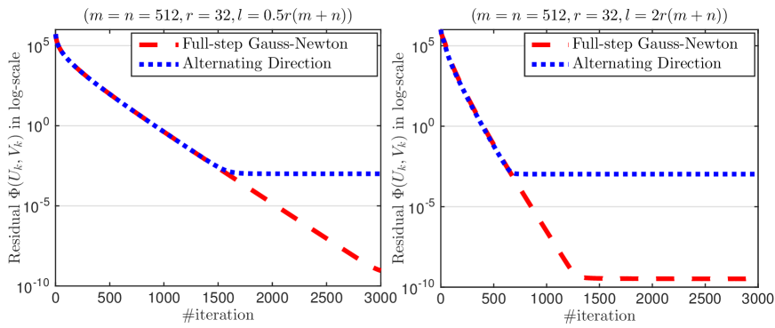
Figure 1. A comparison between FsGN (Legend: Full-step Gauss-Newton) and AMA (Legend: Alternating Direction). Left: The underdetermined case – $l=0.5r(m+n)$. Right: The overdetermined case – $l=2r(m+n)$.

We can see from Figure 1 that both algorithms perform very similarly in early iterations, but then FsGN gives better result in terms of accuracy (terminated around $10^{-9}$ in the overdetermined case due to the nonzero objective residual), while AMA is saturated at a certain level, and does not improve the objective values. In addition, Figures 1 and 2 show that the full-step Gauss-Newton scheme has a local linear convergence rate for the underdetermined case. However, as a compensation, FsGN requires one $(r\times m)$-matrix multiplication $U^{\top}U$ and one $(r\times r)$-inverse compared to AMA. This suggests that we can perform AMA in early iterations and switch to FsGN if AMA does not make significant progress to improve the objective values.

We test the underdetermined case by choosing a Gaussian operator $\mathcal{A}$ generated as $\mathcal{A}=\frac{1}{\sqrt{l}}\texttt{sprandn}(l,mn,0.05)$. The convergence of two algorithms on this dataset is plotted in Figure 2 (left). Finally, we consider the effect of noise to both algorithms by adding a Gaussian noise with $\sigma^{2}=10^{-3}$. The performance of these algorithms is plotted in Figure 2 (right).

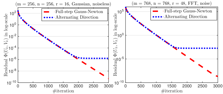
Figure 2. A comparison between FsGN and AMA. Left: sparse Gaussian operator without noise. Right: subsampling FFT linear operator with noise.

We can observe from Figure 2 the same behavior as in the previous test. Our FsGN still maintains a local linear convergence even with noise, while AMA is saturated at a certain level of the objective values.

6.3. Low-rank matrix factorization and linear subspace selection

We consider a special case of (1.1) by taking $\phi(\cdot):=(1/2)\|\cdot\|_{F}^{2}$ and $\mathcal{A}=\mathbb{I}$ as

$$\Phi^{\star}:=\min_{U,V}\left\{\Phi(U,V):=(1/2)\|UV^{\top}-B\|_{F}^{2}\ :\ U\in\mathbb{R}^{m\times r},V\in\mathbb{R}^{n\times r}\right\}.$$ (6.6)

Although this problem has a closed form solution by truncated SVD, our objective is to compare the full-step GN variant of Algorithm 1 with standard Matlab singular value decomposition routines: svds and lansvd. The full-step GN scheme for (6.6) is presented as

$$V_{k+1}^{\top}:=U_{k}^{\dagger}B\quad\text{and}\quad U_{k+1}:=U_{k}+(B-U_{k}^{\top}V_{k+1})(V_{k}^{\dagger})^{\top}.$$ (6.7)

At each iteration, (6.7) requires two $(r\times r)$-matrix inverses $U_{k}^{\top}U_{k}$ and $V_{k}^{\top}V_{k}$, and three $(m\times r)$- or $(n\times r)$- matrix - $(r\times r)$-matrix multiplications. We compute these two inverses by Cholesky decomposition. We note that we do not form the $(m\times n)$-matrix $U_{k}V_{k}^{\top}$ at each iteration, but we can occasionally compute it to check the objective value if required. We choose $U_{0}:=[\mathbb{I}_{r},\boldsymbol{0}_{(m-r)\times r}^{\top}]^{\top}$ and $V_{0}:=[\boldsymbol{0}_{(n-r)\times r}^{\top},\mathbb{I}_{r}]^{\top}$ as a starting point, where $\mathbb{I}_{r}$ is the identity matrix.

Scheme (6.7) generates two low-rank matrices $U_{k}$ and $V_{k}$ so that $U_{k}V_{k}^{\top}\approx B$. We can perform a Rayleigh–Ritz (RR) routine to orthonormalize $U_{k}$ and $V_{k}$,

• Compute $[Q_{u},R_{u}]=\texttt{qr}(U_{k},0)$ and $[Q_{v},R_{v}]=\texttt{qr}(V_{k},0)$, the two economic QR-factorizations of size $r$.

• Compute $[U_{r},\Sigma_{r},V_{r}]=\texttt{svd}(Q_{u}^{\top}BQ_{v})$ the singular value decomposition of the $r\times r$ matrix $Q_{u}^{\top}BQ_{v}$.

• Then form $U=Q_{u}U_{r}$ and $V=Q_{v}V_{r}$ to obtain two orthogonal matrices $U$ and $V$ of the size $m\times r$ and $n\times r$ so that $[U,\Sigma,V]=\texttt{svds}(B,r)$.

Here, (6.7) works on a symmetric positive definite matrix compared to [32].

Now, we test (6.7) in combining with the Rayleigh–Ritz procedure, and compare it with svds and lansvd. We generate an input matrix $B$ of size $m\times n$ with rank $r$. Once $m$ is chosen, we set $n=m$ and either $r=0.01\times m$ or $r=0.05\times m$ (which is either $1\%$ or $5\%$ of the problem size, respectively). Then, we generate $B\in\mathbb{R}^{m\times n}$ using the following Matlab code:

min_mn      = min(m, n);
nnz_sig_vec = [1:1:r].^(-0.01);
sig_vec     = [nnz_sig_vec(:); zeros(min_mn-r, 1)];
n_sig_vec   = sqrt(length(sig_vec))/norm(sig_vec(:), 2)*sig_vec;
B           = gallery(’randcolu’, n_sig_vec, max(m, n), 1);
G           = sprandn(m, n, nnz(B)/(m*n));
M_mat       = B + 0.1*norm(B, ’fro’)*G/norm(G, ’fro’);

Clearly, the singular values $\sigma_{i}$ of $B$ are clustered into two parts: $\sigma_{i}=i^{-0.01}$ for $i=1,\cdots,r$, and $\sigma_{i}=0$ for $i=r+1,\cdots,\min\left\{m,n\right\}$. In addition, an i.i.d. Gaussian noise $\frac{\left\|B\right\|_{F}}{10\left\|G\right\|_{F}}G$ is added to $B$, where $G=\mathcal{N}(0,\sigma\mathbb{I})$, with $\sigma$ being the sparsity of $B$. We terminate (6.7) using either (6.1) or (6.2) with $\varepsilon_{1}=10^{-6}$ or $\varepsilon_{2}=10^{-4}$, respectively. We also terminate svds and lansvd using $\texttt{tol}=10^{-4}$, which is a moderate accuracy.

The performance of three algorithms in terms of computational time vs. problem size is plotted in Figure 3 for $10$ problems from $m=n=1,000$ to $m=n=10,000$, carried out on a MacBook laptop with a 2.6 GHz Intel Core i7 processor and 16GB memory. We run each problem size $10$ times and compute the averaging computational time. The abbreviation Full-step Gauss-Newton indicates the time of both scheme (6.7) and Rayleigh-Ritz procedure, while Full-step Gauss-Newton without RR only counts for the time of (6.7). Figure 3 (left) shows the performance with $r=0.01\times m$, while Figure 3 (right) reveals the case $r=0.05\times m$.

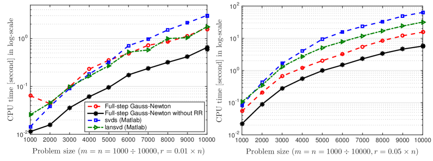
Figure 3. A comparison between the full-step GN scheme, $\mathtt{Matlab~{}SVDS}$, and $\mathtt{Matlab~{}LanSVD}$ on $10$ problem sizes $($from $1,000$ to $10,000$$)$, and two different ranks. The result is on the average of $10$ random runs for each problem size.

When the rank $r$ is about $1\%$ of the problem size, (6.7) is comparable to lansvd while it is slightly better than svds. However, when the rank $r$ is increased to $5\%$ of the problem size, (6.7) clearly outperforms both lansvd and svds.

6.4. Recovery with Pauli measurements in quantum tomography

We consider a $d$ spin-1/2 system with unknown state $S$ as described in [22]. A $d$-qubit Pauli matrix is given by the form $w=\otimes_{i=1}^{d}w_{i}$, where $w_{i}\in\left\{\boldsymbol{1},\sigma^{x},\sigma^{y},\sigma^{z}\right\}$ is a given set of elements. There are $n^{2}$, $n=2^{d}$, such matrices denoted by $w(s)$ with $s\in\left\{1,\cdots,n^{2}\right\}$. A compressive sensing procedure takes $m$ integer numbers $s_{1},\cdots,s_{m}\in\left\{1,\cdots,n^{2}\right\}$ randomly and measures the expected values $\mathrm{trace}\left(Sw(s_{i})\right)$. Then, it solves the following convex problem to construct the unknown states:

$$\mathrm{trace}\left(X\right)=1,\quad\mathrm{trace}\left(Xw(s_{i})\right)=\mathrm{trace}\left(w_{i}S\right)\quad(i=1,\cdots,m).$$ (6.8)

From [22], the number of measurement $m$ to reconstruct the quantum states can be estimated as $m=cnr\log^{2}n\ll n^{2}$ for some constant $c$ and the rank $r$.

Given that $X$ characterizes a density matrix, which is positive semidefinite Hermitian, we instead consider the following least-squares formulation of (6.8):

$$\min_{X\in\mathcal{H}^{n}_{+}}\left\{(1/2)\|B-\mathcal{A}(X)\|_{F}^{2}\ :\ \mathrm{trace}(X)=1\right\},$$ (6.9)

where $\mathcal{H}^{n}_{+}$ is the set of positive semidefinite Hermitian matrices of size $n$, and $\mathcal{A}$ and $B$ are the measurement operator and observed measurements obtained from (6.8), respectively. Assume that $X=UU^{\top}$, where $U\in\mathbb{C}^{n\times 1}$, we can write (6.9) into

$$\min_{U\in\mathbb{C}^{n\times 1}}\left\{(1/2)\|B-\mathcal{A}(UU^{\top})\|_{F}^{2}\right\},$$ (6.10)

where $\mathbb{C}^{n\times 1}$ is the set of $(n\times 1)$ - complex matrices. Clearly, problem (6.10) falls into the special form (5.1) of (1.1) which can be solved by Algorithm 3.

Table 1. Numerical results of three algorithms on noiseless and noisy data

			Algorithm 3			Frank-Wolfe without LS			Frank-Wolfe with LS
#qubits	$m$	$n$	iter	time[s]	$\frac{\left\|B-\mathcal{A}(X)\right\|_{F}}{\left\|B\right\|_{F}}$	iter	time[s]	$\frac{\left\|B-\mathcal{A}(X)\right\|_{F}}{\left\|B\right\|_{F}}$	iter	time[s]	$\frac{\left\|B-\mathcal{A}(X)\right\|_{F}}{\left\|B\right\|_{F}}$
The noiseless case
10	14196	1024	26	12.25	3.21e-06	1707	664.90	1.65e-03	322	129.35	1.62e-03
11	31231	2048	25	71.60	2.64e-06	1654	2803.18	1.61e-03	370	593.56	1.54e-03
12	68140	4096	25	696.27	1.78e-06	1577	17990.98	1.56e-03	254	1741.19	1.54e-03
13	147635	8192	27	1516.97	1.73e-06	648	20574.13	3.68e-03	303	9654.69	1.52e-03
The depolarizing noisy case (1%)
10	14196	1024	24	16.07	8.99e-06	1711	692.16	1.66e-03	238	78.22	1.66e-03
11	31231	2048	23	94.98	8.80e-06	1663	2683.90	1.62e-03	258	423.27	1.61e-03
12	68140	4096	23	589.73	6.03e-06	1585	12146.01	1.56e-03	247	1892.66	1.56e-03
13	147635	8192	24	3684.57	8.76e-06	648	20537.15	3.70e-03	292	8691.90	1.53e-03

We test Algorithm 3 and compared it with Frank-Wolfe’s method proposed in [25]. We use both the standard Frank-Wolfe and its linesearch variant. We generate $U_{0}:=[\mathbb{I}_{r},\boldsymbol{0}_{(n-r)\times r}^{\top}]^{\top}$ and terminate Algorithm 3 using either (6.1), (6.2), or (6.4) with $\varepsilon_{1}=10^{-9}$ and $\varepsilon_{2}=10^{-6}$, respectively. We generate $\mathcal{A}$ and $B$ using the procedures in [22]. We perform two cases: noise and noiseless. In the noisy case, we set $S$ to be $0.99S+0.01\mathbb{I}_{n}/n$ before computing the observed measurement $B$. Since Frank-Wolfe’s algorithms take long time to reach a high accuracy, we terminate them if $\left\|\mathcal{A}(X)-B\right\|_{F}\leq 10^{-3}\sqrt{2}\left\|B\right\|_{F}$ which is different from Algorithm 3.

We test on 4 problems of the size $d$ with $d\in\left\{10,11,12,13\right\}$ being the number of qubits running one a single node of an Intel(R) Xeon(R) 2.67GHz cluster with 4GB memory, but can share up to 320GB RAM. The results and performance of three algorithms are reported in Table 1, where $m$ is the number of measurements, $n=2^{d}$, iter is the number of iterations, time[s] is the computational time in seconds. The convergence behavior of three algorithms for both noiseless and noisy cases with $d=13$ is also plotted in Figure 4.

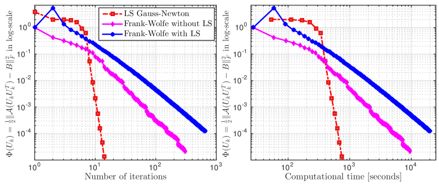
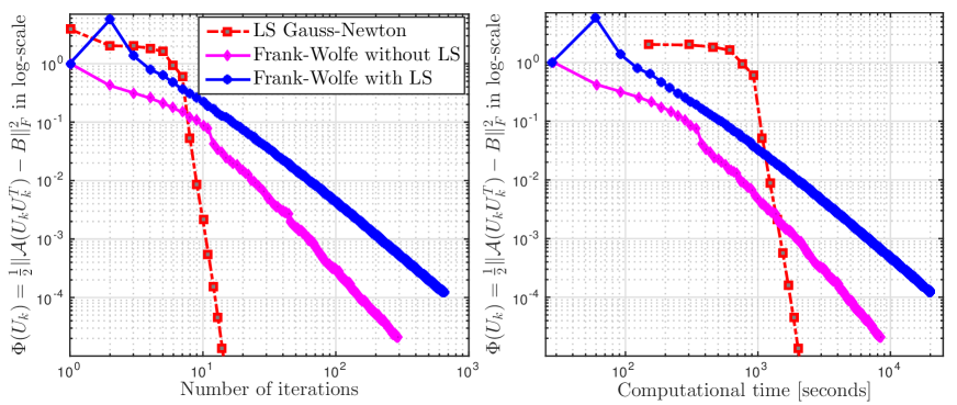
Figure 4. A comparison of three algorithms for the noiseless case (first row) and for the $0.01$ depolarizing noisy case (second row).

We can observe from our results that Algorithm 3 highly outperforms the two Frank-Wolfe variants. It also reaches a highly accurate solution after a few iterations. However, each iteration of Algorithm 3 is more expensive than that of Frank-Wolfe’s algorithms. As can be seen from Figure 4, Algorithm 3 behaves like super-linearly convergent.

6.5. Matrix completion

Our next experiment is solve the well-known matrix completion (MC) widely used in recommender systems [10, 17, 44]. This problem is a special case of (1.1) and can be written as follows:

$$\min_{U,V}\left\{\|(1/2)\mathcal{P}_{\Omega}(UV^{\top})-B\|_{F}^{2}\ :\ U\in\mathbb{R}^{r\times m},V\in\mathbb{R}^{r\times n}\right\},\vspace{-0.75ex}$$ (6.11)

where $\mathcal{P}_{\Omega}$ is a selection operator on an index subset $\Omega$, and $B$ is the set of observed entries.

There are two major approaches to solve (6.11). The first one is using a convex relaxation for the rank constraint via nuclear or max norms. Methods based on this approach have been widely developed, including SVT [8], and [accelerated] gradient descent [17, 40]. The second approach is using nonconvex optimization, including, e.g., OpenSpace [27] and LMaFit [31, 44].

In this experiment, we select the most efficient algorithms for our comparison: the over-relaxation alternating direction method (LMaFit) in [44], and the accelerated proximal gradient method (APGL) in [40]. We will test the four algorithms on synthetic datasets and the three first algorithms on some real datasets.

Synthetic datasets:

Since data in rating systems is often integer, our synthetic dataset is generated as follows. We randomly generate two integer matrices $U$ and $V$ whose entries are in $\left\{1,\cdots,5\right\}$ of the size $m\times r$ and $n\times r$, respectively. Then, we form $M=UV^{\top}$. Finally, we randomly take either $50\%$ or $30\%$ entries of $M$ as an output matrix $B$. We can also add a standard Gaussian noise to $B$ if necessary. A Matlab script for generating such a dataset is given below.

U_org    = randi(5, m, r);
V_org    = randi(5, n, r);
M_org    = U_org*V_org’;
s        = round(0.5*m*n);
Omega    = randsample(m*n, s);
M_omega  = M_org(Omega);
B        = M_omega + sigma*randn(size(M_omega));

We first test these algorithms with a fixed rank $r$ and $50\%$ randomly observed entries, which is relative dense. We terminate Algorithms 1 and 2 using the conditions given in Section 6.1 with $\varepsilon_{1}=10^{-6}$ and $\varepsilon_{2}=10^{-4}$, respectively. We also terminate LMaFit and APGL with the same tolerance $\mathtt{tol}=10^{-4}$. The initial point is computed by a truncated SVD as in Section 6.1.

Table 2. Comparison of four algorithms on synthetic integer data without noise

			Algorithm 1					Algorithm 2
$m$	$n$	$r$	iter	time[s]	$\delta{f}_{k}$	NMAE	rank	iter	time[s]	$\delta{f}_{k}$	NMAE	rank
1000	2000	10	15.9	2.11	4.15e-05	1.39e-05	10	30.0	2.07	8.34e-05	3.55e-05	10
1000	2000	50	20.8	4.34	6.91e-05	5.78e-05	50	37.6	4.43	9.61e-05	7.83e-05	50
2500	2500	25	14.3	8.05	5.31e-05	2.97e-05	25	31.1	9.18	1.04e-04	6.18e-05	25
2500	2500	125	26.3	28.94	7.35e-05	8.18e-05	125	35.2	23.68	1.05e-04	1.32e-04	125
5000	5000	50	15.7	53.40	5.42e-05	3.90e-05	50	32.0	56.71	9.87e-05	7.80e-05	50
5000	5000	250	23.6	180.70	7.94e-05	1.35e-04	250	35.0	165.89	1.10e-04	1.94e-04	250
5000	7500	50	14.9	76.93	5.10e-05	3.64e-05	50	32.0	85.72	8.51e-05	6.65e-05	50
5000	7500	250	23.7	273.30	7.61e-05	1.22e-04	250	35.0	245.93	9.97e-05	1.68e-04	250
10000	10000	100	16.2	289.14	5.99e-05	5.86e-05	100	32.2	319.92	1.10e-04	1.16e-04	100
10000	10000	500	24.8	1303.01	8.02e-05	1.75e-04	500	35.0	1173.38	1.14e-04	2.60e-04	500
			LMaFit [44]					APGL [40]
$m$	$n$	$r$	iter	time[s]	$\delta{f}_{k}$	NMAE	rank	iter	time[s]	$\delta{f}_{k}$	NMAE	rank
1000	2000	10	13.3	0.94	4.74e-05	1.43e-05	10	28.0	4.29	3.31e-04	1.40e-04	10
1000	2000	50	109.8	12.13	2.71e-04	1.51e-04	50	28.6	6.79	1.06e-02	9.02e-03	41.6
2500	2500	25	10.0	3.10	6.98e-05	3.86e-05	25	29.0	16.64	5.06e-04	3.07e-04	25
2500	2500	125	135.3	85.78	2.99e-04	2.59e-04	125	31.6	20.00	1.92e-02	2.43e-02	5
5000	5000	50	10.0	18.43	5.57e-05	4.30e-05	50	30.6	81.69	8.48e-04	6.73e-04	50.2
5000	5000	250	140.9	631.58	6.70e-05	8.58e-05	250	30.4	60.75	1.38e-02	2.44e-02	5
5000	7500	50	10.1	28.21	4.38e-05	2.92e-05	50	30.8	122.47	7.35e-04	5.76e-04	50
5000	7500	250	126.8	845.90	7.02e-05	7.30e-05	250	30.5	90.74	1.38e-02	2.33e-02	5
10000	10000	100	11.0	112.82	3.10e-05	3.24e-05	100	32.7	266.16	2.15e-02	2.28e-02	5
10000	10000	500	120.4	3818.05	6.25e-05	8.63e-05	500	30.3	206.86	9.85e-03	2.26e-02	5

The test is conducted on $10$ problems of different sizes running on a single node of an Intel(R) Xeon(R) 2.67GHz cluster with 4GB memory, but can share up to 100GB RAM. We run each problem size $10$ times and compute the average result and performance. The problem sizes and results are reported in Table 2 for two different ranks. The rank $r$ is chosen as $r=0.01\times m$, and $r=0.05\times m$, which correspond to $1\%$, and $5\%$ of the problem size. Here, iter and time[s] are the number of iterations and the computational time in seconds, respectively; rank is the rank of $U_{k}V_{k}^{\top}$ given by the algorithms; and

$$\delta{f}_{k}:=\|\mathcal{P}_{\Omega}(U_{k}V_{k}^{\top})-B\|_{F}/\left\|B\right\|_{F}\quad\text{and}\quad\mathrm{NMAE}:=C^{-1}\sum_{(i,j)\in\Omega}\big{|}(U_{k}V_{k}^{\top})_{ij}-B_{ij}\big{|},$$

are the relative objective residual; and the Normalized Mean Absolute Error, respectively, where $C:=(\max_{i,j}B_{ij}-\min_{ij}B_{ij})|\Omega|$.

The results in Table 2 show that both Algorithms 1 and 2 produce similar results as LMaFit in terms of the relative objective residual and NMAE. When the rank is small (i.e., $1\%$ of problem size), Algorithm 1 and LMaFit have similar number of iterations, but LMaFit has better computational time. When the rank is increasing up to $5\%$ of the problem size, both Algorithm 1 and Algorithm 2 require a fewer iterations than LMaFit, and outperform this solver in terms of computational time. In this experiment, the number of iterations in Algorithm 2 is very similar in all the test cases, from $30$ to $38$ iterations, and similar to APGL. Note that we fix the rank in the first three algorithms, since APGL uses a convex approach, it cannot predict well an approximate rank if it is $5\%$ of the problem size, or when the problem size is increasing.

Now, we add i.i.d. Gaussian noise $\mathcal{N}(0,\sigma\mathbb{I})$ with $\sigma=0.01$ to $B$ as $B:=B^{\natural}+5\times\mathcal{N}(0,\sigma\mathbb{I})$, and only randomly take $30\%$ observed entries. The convergence behavior of three algorithms for one problem instance with $m=n=5000$ is plotted in Figure 5.

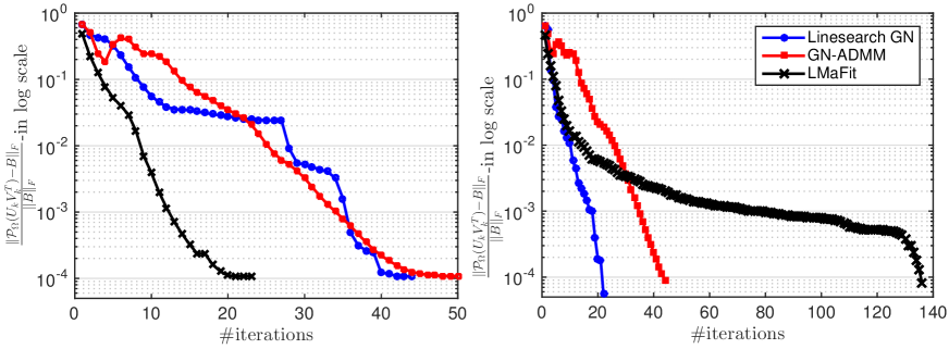
Figure 5. The convergence behavior of three algorithms ($m=n=5000$) with noise ($\sigma=0.01$) and $30\%$ known entries (Left: $r=0.01m$, Right: $r=0.025m$).

When the rank $r=0.01m$ (i.e., $1\%$ of the problem size), LMaFit outperforms Algorithms 1 and 2 in terms of iterations, but when the rank $r=0.025m$ (i.e., $2.5\%$ of the problem size), Algorithms 1 and 2 are much better than LMaFit. Algorithm 1 works really well in the second case, and takes only $22$ iterations. We also observe the monotone decrease in Algorithm 1 as guaranteed by our theory, but not in Algorithm 2.

Table 3. Comparison of the four algorithms on synthetic integer datasets with noise.

			Algorithm 1					Algorithm 2
$m$	$n$	$r$	iter	time[s]	$\delta{f}_{k}$	NMAE	rank	iter	time[s]	$\delta{f}_{k}$	NMAE	rank
1000	2000	10	40.8	3.56	5.33e-04	2.27e-04	10	40.5	2.24	5.32e-04	2.26e-04	10
1000	2000	25	49.1	5.50	6.05e-04	2.76e-04	25	62.0	4.62	2.09e-04	1.31e-04	25
5000	5000	50	19.5	39.82	1.10e-04	8.71e-05	50	45.0	67.70	1.09e-04	8.63e-05	50
5000	5000	125	16.6	56.70	7.90e-05	9.58e-05	125	40.0	103.45	9.50e-05	1.19e-04	125
			LMaFit [44]					APGL [40]
$m$	$m$	$r$	iter	time[s]	$\delta{f}_{k}$	NMAE	rank	iter	time[s]	$\delta{f}_{k}$	NMAE	rank
1000	2000	10	31.6	1.71	5.31e-04	2.26e-04	10	28.0	3.08	6.34e-04	2.70e-04	10
1000	2000	25	121.0	8.55	2.08e-04	1.31e-04	25	30.7	5.86	9.87e-04	5.93e-04	25
5000	5000	50	20.0	30.39	1.07e-04	8.49e-05	50	28.5	52.96	4.97e-03	3.82e-03	48.2
5000	5000	125	48.0	121.11	7.19e-05	7.34e-05	125	31.3	46.99	1.92e-02	2.42e-02	5

Finally, we test three first algorithms on two problem instances with $30\%$ observed entries in $B$ and with i.i.d. Gaussian noise $\mathcal{N}(0,0.01\mathbb{I})$). The results of this test is reported in Table 3. LMaFit remains working well for then low-rank cases, while getting slower when the rank $r$ increases. Algorithms 1 and 2 have similar performance in this case.

Real datasets:

Now, we test three algorithms: Algorithms 1 and 2, and LMaFit on MovieLens and Jester jokes datasets available on http://grouplens.org/datasets/movielens/. For the MovieLens dataset, we test our algorithms on $5$ problems: “movie-lens-latest (small)”, “movie-lens” 100k, 1M, 10M, and 20M, which we abbreviate by “movie(s)”, and “moviexM” in Table 4, respectively. We also test all problems in Jester joke dataset: “jester-1”, “jester-2”, “jester-3”, and “jester-all”.

Table 4. Summary of results of four the algorithms for MC on “real” datasets

			Algorithm 1			Algorithm 2			LMaFit [44]
Name	$m$	$n$	iter	time[s]	$\delta{f}_{k}$	iter	time[s]	$\delta{f}_{k}$	iter	time[s]	$\delta{f}_{k}$
jester-1	24983	100	45	11.60	1.75e-01	59	11.35	1.75e-01	36	4.78	1.75e-01
jester-2	23500	100	41	9.93	1.77e-01	57	11.07	1.77e-01	34	5.51	1.77e-01
jester-3	24938	100	30	5.15	9.04e-04	32	4.94	9.66e-04	25	2.13	9.26e-04
jester-all	73421	100	48	35.12	1.65e-01	57	30.12	1.65e-01	36	12.21	1.65e-01
movie(s)	668	10325	200	16.69	1.64e-03	87	7.14	1.58e-03	200	44.18	1.58e-03
movie100k	943	1682	200	9.66	1.03e-02	84	4.87	1.00e-02	200	15.63	1.00e-02
movie1M	6040	3706	79	41.71	1.18e-01	42	21.96	1.19e-01	70	49.84	1.18e-01
movie10M	69878	10677	69	109.02	2.14e-01	33	38.32	2.15e-01	61	40.48	2.14e-01
movie20M	138493	26744	89	307.22	2.30e-01	37	117.23	2.30e-01	87	133.86	2.30e-01
			Algorithm 1			Algorithm 2			LMaFit [44]
Name	$m$	$n$	rank	$\delta{x}_{k}$	NMAE	rank	$\delta{x}_{k}$	NMAE	rank	$\delta{x}_{k}$	NMAE
jester-1	24983	100	80	4.71e-01	2.29e-02	80	4.71e-01	2.36e-02	80	4.59e-01	2.30e-02
jester-2	23500	100	80	4.82e-01	2.35e-02	80	4.82e-01	2.42e-02	80	4.78e-01	2.39e-02
jester-3	24938	100	80	8.78e-04	1.08e-05	80	8.78e-04	7.22e-05	80	9.87e-04	2.08e-05
jester-all	73421	100	80	4.09e-01	1.95e-02	80	4.09e+01	2.05e-02	80	3.95e-01	1.98e-02
movie(s)	668	10325	100	1.36e-01	3.76e-04	100	1.36e-01	6.91e-04	100	1.36e-01	3.97e-04
movie100k	943	1682	100	1.10e-04	5.24e-03	100	1.10e-04	4.87e-03	100	1.00e-04	4.64e-03
movie1M	6040	3706	100	2.34e-01	8.28e-02	100	2.34e-01	8.44e-02	100	2.32e-01	8.32e-02
movie10M	69878	10677	20	5.86e-01	1.34e-01	20	5.86e-01	1.35e-01	20	5.81e-01	1.34e-01
movie20M	138493	26744	10	6.29e-01	1.42e-01	10	6.29e-01	1.42e-01	10	6.30e-01	1.42e-01

In this test, since the data in “movie10M” and “movie20M” is sparse, we run the three algorithms on a MacBook laptop with a 2.6 GHz Intel Core i7 processor and 16GB memory. We use C-mex routines in Matlab to compute $\mathcal{P}_{\Omega}(UV^{\top})$ in three algorithms to avoid forming $U^{\top}V$. We terminates our algorithms based on the objective obtained from LMaFit such that the three algorithms have similar objective values.

The result is summarized in Table 4, where we add a new measurement defined by $\delta{x}_{k}:=\frac{1}{|\Omega|}\sum_{(i,j)\in\Omega}\left|\lfloor(U_{k}V_{k}^{\top})_{ij}\rfloor-B_{ij}\right|$ to measure the agreement ratio between the recovered matrix $M_{k}:=U_{k}V_{k}^{\top}$ and the observed data $B$ projected onto $\Omega$. Due to our stopping criterion, three algorithms produce similar results in terms of the objective residuals, solution agreement, and NMAE. LMaFit works well on the Jester jokes dataset, but the computational time on these problems is relatively small. Algorithm 2 works well on Movielen dataset, especially for Movie 10MB and Movie 20MB. As mentioned previously, Algorithm 1 often achieve better solution in terms of accuracy if we run it long enough, while LMaFit and Algorithm 2 can be used to achieve a low or medium accurate solution for matrix completion.

6.6. Robust low-rank matrix recovery

We consider the following nonsmooth problem in low-rank matrix recovery:

$$\min_{U,V}\left\{\|UV^{\top}-B\|_{1}\ :\ U\in\mathbb{R}^{m\times r},V\in\mathbb{R}^{n\times r}\right\},$$ (6.12)

where $\left\|Z\right\|_{1}:=\sum_{ij}\left|Z_{ij}\right|$ is the $\ell_{1}$-norm of $Z$. This a low-rank matrix recovery problem with the $\ell_{1}$-norm, which can be referred to as a robust recovery as opposed to the standard square loss. This formulation is often used in background extraction, see, e.g., [38].

Clearly, we can solve (6.12) using our ADMM-GN scheme above, which can be written as

$$\left\{\begin{array}[]{lcl}V_{k+1}^{\top}&:=&U_{k}^{\dagger}(B+W_{k}-\Lambda_{k}),\vspace{1ex}\\ U_{k+1}&:=&U_{k}+\left(B+W_{k}-\Lambda_{k}-U_{k}V_{k+1}^{\top}\right)(V_{k}^{\dagger})^{\top},\vspace{1ex}\\ W_{k+1}&:=&\mathrm{prox}_{\rho^{-1}\left\|\cdot\right\|_{1}}\left(U_{k+1}V_{k+1}^{\top}+\Lambda_{k}-B\right)\vspace{1ex}\\ \Lambda_{k+1}&:=&\Lambda_{k}+(U_{k+1}V_{k+1}^{\top}-W_{k+1}).\end{array}\right.$$ (6.13)

We apply this scheme to solve the (6.12) using video surveillance datasets at http://perception.i2r.a-star.edu.sg/bk_model/bk_index.html. We implement (6.13) in Algorithm 2 and compare it with the augmented Lagrangian method proposed in [38], which we denote by L1-LMaFit. We use the same strategy as in L1-LMaFit to update the penalty parameter $\rho$, while using $U_{0}:=[\mathbb{I}_{r},\boldsymbol{0}_{(m-r)\times r}]$ and $V_{0}:=[\mathbb{I}_{r},\boldsymbol{0}_{(n-r)\times r}]$ as an initial point. As suggested in [38], we choose the rank $r$ to be $r=1$ when testing gray-scale video data. As experienced, L1-LMaFit was based on alternating minimization idea, which can be saturated. Hence, we run both algorithm up to $100$ iterations to observe the outcome. The computational time and the relative objective value $\|U_{k}V_{k}^{\top}-B\|_{1}/\|B\|_{1}$ of these two algorithms are reported in Table 5.

Table 5. Summary of results of the two algorithms for video background extraction.

Video data			Algorithm 2		L1-LMaFit [38]
Video	Resolution	#Frames	Time	$\|U_{k}V_{k}^{\top}-B\|_{1}/\|B\|_{1}$	Time	$\|U_{k}V_{k}^{\top}-B\|_{1}/\|B\|_{1}$
Escalator	$130\times 160$	200	12.48	$9.434063\times 10^{-2}$	13.30	$9.435117\times 10^{-2}$
Fountain	$128\times 160$	200	13.27	$4.197912\times 10^{-2}$	13.71	$4.198963\times 10^{-2}$
Bootstrap	$120\times 160$	250	15.76	$13.103802\times 10^{-2}$	16.91	$13.107209\times 10^{-2}$
Curtain	$128\times 160$	250	18.43	$2.965992\times 10^{-2}$	25.45	$2.969248\times 10^{-2}$
Campus	$128\times 160$	300	24.83	$9.315523\times 10^{-2}$	30.10	$9.316343\times 10^{-2}$
Hall	$144\times 176$	300	31.63	$5.708911\times 10^{-2}$	39.05	$5.709121\times 10^{-2}$
ShoppingMall	$256\times 320$	350	82.22	$4.442732\times 10^{-2}$	85.48	$4.442907\times 10^{-2}$
WaterSurface	$128\times 160$	350	35.92	$3.607625\times 10^{-2}$	40.25	$3.607747\times 10^{-2}$

We can observe from Table 5 that the computational time in both algorithms is almost the same. This is consistent with our theoretical result, since the per-iteration complexity of the two algorithms is almost the same when we choose $r=1$. However, Algorithm 2 provides a slightly better objective value since it still improves the objective when running further compared to L1-LMaFit. Here, we use the full-step variant of Algorithm 2, a fast convergence guarantee can be achieved when a good initial point is provided. This remains unclear in L1-LMaFit [38]. Unfortunately, global convergence of our variant as well as L1-LMaFit has not been known yet.

7. Conclusions

We have proposed a new Gauss-Newton scheme to approximate a stationary point of a class of low-rank matrix nonconvex optimization problems. Our method features several advantages from classical Gauss-Newton (GN) method such as fast local convergence, achieving high accuracy solutions compared to the well-known alternating minimization algorithm (AMA). We have proposed a linesearch GN algorithm and established its global and local convergence under standard assumptions. We have also specified this algorithm to the symmetric case, where AMA is not applicable. Then, we have combined our GN scheme with the alternating direction method of multipliers (ADMM) to design a new ADMM-GN algorithm that has global convergence guarantee and low per-iteration complexity. Several numerical experiments have been presented to demonstrate the theory and show the advantages of nonconvex optimization approaches. The theory and algorithms presented in this paper can be extended to different directions, including constrained low-rank matrix/tensor optimization.

Acknowledgments. The author was partly supported by the Office of Naval Research under Grant No. ONR-N00014-20-1-2088. The author would like to thank Dr. Zheqi Zhang for proving some Matlab codes to conduct the experiments in Subsection 6.2.

Appendix A The proof of technical results

We provide the full proofs of all the technical results in the main text.

A.1. The proof of Lemma 3.1: Closed form of Gauss-Newton direction

Le us define $x:=[\mathrm{vec}\left(D_{V}^{\top}\right),\mathrm{vec}\left(D_{U}\right)]$ and $b:=[\mathrm{vec}(U^{\top}B),\mathrm{vec}(BV)]$. Then, we can write (3.5) as $\mathcal{B}x=b$, where $\mathcal{B}:=\begin{bmatrix}\mathbb{I}_{n}\otimes U^{\top}U&V\otimes U^{\top}\\ V^{\top}\otimes U&V^{\top}V\otimes\mathbb{I}_{m}\end{bmatrix}$. We can show that

$$\mathcal{B}=\begin{bmatrix}(\mathbb{I}_{n}\otimes U^{\top})(\mathbb{I}_{n}\otimes U)&(\mathbb{I}_{n}\otimes U^{\top})(V\otimes\mathbb{I}_{m})\\ (V^{\top}\otimes\mathbb{I}_{m})(\mathbb{I}_{n}\otimes U)&(V^{\top}\otimes\mathbb{I}_{m})(V\otimes\mathbb{I}_{m})\end{bmatrix}=\begin{bmatrix}\mathbb{I}_{n}\otimes U^{\top}\\ V^{\top}\otimes\mathbb{I}_{m}\end{bmatrix}\begin{bmatrix}\mathbb{I}_{n}\otimes U&V\otimes\mathbb{I}_{m}\end{bmatrix}.$$

By [1, Fact. 7.4.24], we have $\mathrm{rank}\left([\mathbb{I}_{n}\otimes U,V\otimes\mathbb{I}_{m}]\right)\leq(m+n-r)r$. Hence, $\mathrm{rank}\left(\mathcal{B}\right)$ in (3.5) does not exceed $r(m+n-r)<r(m+n)$.

Next, we can rewrite $b=[(\mathbb{I}_{n}\otimes U^{\top})\mathrm{vec}(B);(V^{\top}\otimes\mathbb{I}_{m})\mathrm{vec}(B)]$. If we consider the extended matrix $\bar{\mathcal{B}}:=[\mathcal{B},b]$, then we can express it as

$$\bar{\mathcal{B}}=\begin{bmatrix}\mathbb{I}_{n}\otimes U^{\top}\\ V^{\top}\otimes\mathbb{I}_{m}\end{bmatrix}\begin{bmatrix}\mathbb{I}_{n}\otimes U&V\otimes\mathbb{I}_{m}&\mathrm{vec}(B)\end{bmatrix}.$$

This shows that $\mathrm{rank}\left(\bar{\mathcal{B}}\right)=\mathrm{rank}\left(\mathcal{B}\right)$. Hence, by the well-known consistency Rouché–Capelli theorem, (3.5) has a solution.

Now, we find the closed form (3.7). Since $\mathrm{rank}\left(U\right)=\mathrm{rank}\left(V\right)=r$, both $U^{\top}U$ and $V^{\top}V$ are invertible. Pre-multiplying the first equation of (3.5) by $(U^{\top}U)^{-1}$ and rearranging the result, we have

$$D_{V}^{\top}=(U^{\top}U)^{-1}U^{\top}(Z-D_{U}V^{\top}).$$ (A.1)

Substituting this expression into the second equation of (3.5) we get

$$(\mathbb{I}-U(U^{\top}U)^{-1}U^{\top})D_{V}V^{\top}V=(\mathbb{I}-U(U^{\top}U)^{-1}U^{\top})ZV.$$ (A.2)

Using the definition of the projections $P_{U}$, $P_{V}$, $P^{\perp}_{U}$ and $P^{\perp}_{V}$, we have from (A.2) that $P^{\perp}_{U}D_{V}V^{\top}V=P^{\perp}_{U}ZV$. Post-multiplying this expression by $(V^{\top}V)^{-1}$, we obtain

$$P^{\perp}_{U}D_{V}=P^{\perp}_{U}ZV(V^{\top}V)^{-1}.$$ (A.3)

Assume that $D_{U}:=D_{U}^{0}+U\hat{D}_{r}$, where $D_{U}^{0}$ is a given vector in the null space of $U^{\top}$, i.e., $U^{\top}D_{U}^{0}=0$, and $\hat{D}_{r}\in\mathbb{R}^{r\times r}$ is an arbitrary matrix. Substituting this expression into (A.3) and noting that $P^{\perp}_{U}U=0$, we obtain

$$D_{U}^{0}=D_{U}^{0}-U(U^{\top}U)^{-1}U^{\top}D_{U}^{0}+P^{\perp}_{U}U\hat{D}_{r}=P^{\perp}_{U}ZV(V^{\top}V)^{-1}.$$

Hence, we finally get

$$D_{U}=P^{\perp}_{U}ZV(V^{\top}V)^{-1}+U\hat{D}_{r},~{}~{}\text{for any}~{}\hat{D}_{r}\in\mathbb{R}^{r\times r},$$

which is exactly the first term in (3.6). Substituting this $D_{U}$ into (A.1) to yield the second term of (3.6) as

$$\begin{array}[]{lcl}D^{\top}_{V}&=&(U^{\top}U)^{-1}U^{\top}\left(Z-P^{\perp}_{U}ZV(V^{\top}V)^{-1}V^{\top}-U\hat{D}_{r}V^{\top}\right)\vspace{1ex}\\ &=&(U^{\top}U)^{-1}U^{\top}Z-U^{\top}U)^{-1}U^{\top}P^{\perp}_{U}ZV(V^{\top}V)^{-1}V^{\top}-\hat{D}_{r}V^{\top}\vspace{1ex}\\ &=&(U^{\top}U)^{-1}U^{\top}Z-\hat{D}_{r}V^{\top}.\end{array}$$

Since $\hat{D}_{r}$ is arbitrary in $\mathbb{R}^{r\times r}$, we choose $\hat{D}_{r}:=\frac{1}{2}(U^{\top}U)^{-1}U^{\top}ZV(V^{\top}V)^{-1}\in\mathbb{R}^{r\times r}$. Substituting this choice into (3.6), we obtain

$$D_{U}=\big{(}\mathbb{I}_{m}-(1/2)P_{U}\big{)}ZV(V^{\top}V)^{-1}\quad\text{and}\quad D_{V}^{\top}=(U^{\top}U)^{-1}U^{\top}Z\big{(}\mathbb{I}_{n}-(1/2)P_{V}\big{)},$$

which is (3.7). Hence, the solution set of (3.5) forms an $(r\times r)$-linear subspace.

Finally, let us denote the residual term in the objective of (3.4) by $R(D_{U},D_{V}):=UD_{V}^{\top}+D_{U}V^{\top}-Z$. Then, using the expression (3.6) we can easily show that

$$\begin{array}[]{lcl}R(D_{U},D_{V})&=&U((U^{\top}U)^{-1}U^{\top}Z-\hat{D}_{r}V^{\top})+(P^{\perp}_{U}ZV(V^{\top}V)^{-1}+U\hat{D}_{r})V^{\top}-Z\vspace{1ex}\\ &=&P_{U}Z+P^{\perp}_{U}ZP_{V}-P_{U}Z-P^{\perp}_{U}Z=P^{\perp}_{U}ZP_{V}-P^{\perp}_{U}Z.\end{array}$$

Hence, we can write

$$R(D_{U},D_{V})=-P^{\perp}_{U}ZP^{\perp}_{V}\quad\text{and}\quad(1/2)\|R(D_{U},D_{V})\|_{F}^{2}=(1/2)\|P^{\perp}_{U}ZP^{\perp}_{V}\|_{F}^{2}.$$

The last term $(1/2)\|P^{\perp}_{U}ZP^{\perp}_{V}\|_{F}^{2}$ is the optimal value of (3.4). $\square$

A.2. The proof of Lemma 3.2: Descent property of GN algorithm

Let us define $U(\alpha):=U+\alpha D_{U}$ and $V(\alpha):=V+\alpha D_{V}$ for $\alpha>0$. Then

$$U(\alpha)V(\alpha)^{\top}=UV^{\top}+\alpha(UD_{V}^{\top}+D_{U}V^{\top})+\alpha^{2}D_{U}D_{V}^{\top}.$$ (A.4)

Let $W:=UD_{V}^{\top}+D_{U}V^{\top}$ and $r(\alpha):=\|U(\alpha)V(\alpha)^{\top}-UV^{\top}-Z\|_{F}^{2}$. Using (A.4) we have

$$\begin{array}[]{lcl}r(\alpha)&=&\|\alpha(UD_{V}^{\top}+D_{U}V^{\top})+\alpha^{2}D_{U}D_{V}^{\top}-Z\|^{2}_{F}\vspace{1ex}\\ &=&\|Z\|_{F}^{2}+\alpha^{2}\|W\|^{2}_{F}+\alpha^{4}\|D_{U}D_{V}^{\top}\|_{F}^{2}+2\alpha^{3}\langle W,D_{U}D_{V}^{\top}\rangle-2\alpha\langle W,Z\rangle-2\alpha^{2}\langle Z,D_{U}D_{V}^{\top}\rangle.\end{array}$$

Now, using the fact that

$$\langle W,Z-W\rangle =\langle UD_{V}^{\top}+D_{U}V^{\top},P^{\perp}_{U}ZP^{\perp}_{V}\rangle=\mathrm{trace}\left((D_{V}U^{\top}+VD_{U}^{\top})P^{\perp}_{U}ZP^{\perp}_{V}\right)=0,$$

we can further expand $r(\alpha)$ as

$$\begin{array}[]{lcl}r(\alpha)&=&\|Z\|_{F}^{2}-\alpha(2-\alpha)\|W\|^{2}_{F}+\alpha^{4}\|D_{U}D_{V}^{\top}\|_{F}^{2}\vspace{1ex}\\ &&-{~{}}2\alpha^{2}(1-\alpha)\langle W,D_{U}D_{V}^{\top}\rangle+2\alpha^{2}\langle W-Z,D_{U}D_{V}^{\top}\rangle.\end{array}$$ (A.5)

Using the pseudo-inverse of $U$ and $V$ and $(V^{\top})^{\dagger}U^{\dagger}=(UV^{\top})^{\dagger}$, we can show that

$$D_{U}D_{V}^{\top} =\big{(}\mathbb{I}_{m}-0.5P_{U}\big{)}Z(UV^{\top})^{\dagger}Z\big{(}\mathbb{I}_{n}-0.5P_{V}\big{)}.$$

From the optimality condition (2.1) and the definition of $Z=-L_{\Phi}^{-1}\mathcal{A}^{*}\nabla{\phi}(\mathcal{A}(UV^{\top})-B))$, we can show that $\nabla_{U}{\Phi}(U,V)=-L_{\Phi}U^{\top}Z$ and $\nabla_{V}{\Phi}(U,V)=-L_{\Phi}ZV$. However, since $D_{U}$ and $D_{V}$ are given by (3.7), we express

$$\left\{\begin{array}[]{lcl}D_{U}&=&-\frac{1}{L_{\Phi}}\big{(}P^{\perp}_{U}+\frac{1}{2}P_{U}\big{)}\nabla_{U}{\Phi}(U,V)(V^{\top}V)^{-1},\vspace{1ex}\\ D_{V}^{\top}&=&-\frac{1}{L_{\Phi}}(U^{\top}U)^{-1}\nabla_{V}{\Phi}(U,V)\big{(}P^{\perp}_{V}+\frac{1}{2}P_{V}\big{)}.\end{array}\right.$$

Using this expression, we can write $\nu:=\left\|D_{U}\right\|_{F}^{2}+\left\|D_{V}\right\|_{F}^{2}$ as

$$\nu=\frac{1}{L_{\Phi}^{2}}\|\big{(}P^{\perp}_{U}+\frac{1}{2}P_{U}\big{)}\nabla_{U}{\Phi}(U,V)(V^{\top}V)^{-1}\|_{F}^{2}+\frac{1}{L_{\Phi}^{2}}\|(U^{\top}U)^{-1}\nabla_{V}{\Phi}(U,V)\big{(}P^{\perp}_{V}+\frac{1}{2}P_{V}\big{)}\|_{F}^{2}.$$

Hence, we can estimate

$$\frac{\|\nabla_{U}{\Phi}(U,V)\|_{F}^{2}}{4L_{\Phi}^{2}(\sigma_{\max}(V))^{4}}+\frac{\|\nabla_{V}{\Phi}(U,V)\|_{F}^{2}}{4L_{\Phi}^{2}(\sigma_{\max}(U))^{4}}\leq\nu\leq\frac{\|\nabla_{U}{\Phi}(U,V)\|_{F}^{2}}{L_{\Phi}^{2}(\sigma_{\min}(U))^{4}}+\frac{\|\nabla_{V}{\Phi}(U,V)\|_{F}^{2}}{L_{\Phi}^{2}(\sigma_{\min}(V))^{4}},$$ (A.6)

where $\sigma_{\min}(\cdot)$ and $\sigma_{\max}(\cdot)$ are the smallest and largest singular values of $(\cdot)$, respectively. Let $\sigma_{\max}:=\max\left\{\sigma_{\max}(U),\sigma_{\max}(V)\right\}$ and $\sigma_{\min}:=\min\left\{\sigma_{\min}(U),\sigma_{\min}(V)\right\}$. Using $\|\nabla{\Phi}(U,V)\|_{F}^{2}=\|\nabla_{U}{\Phi}(U,V)\|_{F}^{2}+\|\nabla_{V}{\Phi}(U,V)\|_{F}^{2}$, (A.6) leads to

$$\frac{\|\nabla{\Phi}(U,V)\|_{F}^{2}}{4L_{\Phi}^{2}\sigma_{\max}^{4}}\leq\nu=\left\|D_{U}\right\|_{F}^{2}+\left\|D_{V}\right\|_{F}^{2}\leq\frac{\|\nabla{\Phi}(U,V)\|_{F}^{2}}{L_{\Phi}^{2}\sigma_{\min}^{4}}.$$ (A.7)

Next, using the orthonormality, we estimate $\left\|W\right\|_{F}^{2}$ as follows:

$$\begin{array}[]{lcl}\left\|W\right\|_{F}^{2}&=&\|UD_{V}^{\top}+D_{U}V^{\top}\|_{F}^{2}=\|UD_{V}^{\top}\|_{F}^{2}+\|D_{U}V^{\top}\|_{F}^{2}\vspace{1ex}\\ &=&\mathrm{trace}\left(D_{V}(U^{\top}U)D_{V}^{\top}\right)+\mathrm{trace}\left(D_{U}(V^{\top}V)D_{U}^{\top}\right)\vspace{1ex}\\ &\geq&(\sigma_{\min}(U))^{2}\|D_{U}\|_{F}^{2}+(\sigma_{\min}(V))^{2}\|D_{V}\|_{F}^{2}\vspace{1ex}\\ &\geq&\sigma_{\min}^{2}\nu.\end{array}$$ (A.8)

On the one hand, we estimate individually each term of the expression (A.5) as follows:

$$\|D_{U}D_{V}^{\top}\|_{F}^{2} =\mathrm{trace}\left((D_{U}D_{V}^{\top})^{\top}(D_{U}D_{V})\right)\leq\frac{1}{4}\left(\|D_{U}\|_{F}^{2}+\|D_{V}\|_{F}^{2}\right)^{2}=\frac{\nu^{2}}{4}.$$

On the other hand, since $W-Z=-P^{\perp}_{U}ZP^{\perp}_{V}$ by Lemma 3.1, we can show that

$$\langle W-Z,D_{U}D_{V}^{\top}\rangle=\langle P^{\perp}_{U}ZP^{\perp}_{V},D_{U}D_{V}^{\top}\rangle=\mathrm{trace}\left(D_{V}^{\top}P^{\perp}_{V}Z^{\top}P^{\perp}_{U}D_{U}\right)\leq\|Z\|_{F}\|D_{U}D_{V}^{\top}\|_{F}.$$

In addition, $-\langle W,D_{U}D_{V}\rangle\leq\|W\|_{F}\|D_{U}D_{V}^{\top}\|_{F}$. Substituting these estimates into (A.5) and using the fact that $2-\alpha\geq 1$ and $1-\alpha\leq 1$ we obtain

$$\begin{array}[]{lcl}r(\alpha)&\leq&\|Z\|_{F}^{2}-\alpha\|W\|^{2}_{F}+\frac{\nu^{2}\alpha^{4}}{4}+2\alpha^{2}\|W\|_{F}\|D_{U}D_{V}^{\top}\|_{F}+2\alpha^{2}\|Z\|_{F}\|D_{U}D_{V}^{\top}\|_{F}\vspace{1ex}\\ &\leq&\|Z\|_{F}^{2}-\frac{\alpha}{16}\|W\|^{2}_{F}-\frac{\alpha\nu\sigma_{\min}^{2}}{16}+\frac{\nu^{2}\alpha^{4}}{4}-\frac{\alpha}{2}\|W\|_{F}^{2}+2\alpha^{2}\|W\|_{F}\|D_{U}D_{V}^{\top}\|_{F}\vspace{1ex}\\ &&-{~{}}\frac{3\alpha}{8}\|W\|_{F}^{2}+2\alpha^{2}\|Z\|_{F}\|D_{U}D_{V}^{\top}\|_{F}\vspace{1ex}\\ &=&\|Z\|_{F}^{2}-\frac{\alpha\nu\sigma_{\min}^{2}}{16}-\frac{\alpha\nu}{16}\big{(}\sigma_{\min}^{2}-4\alpha^{3}\nu\big{)}_{[b_{1}]}-\frac{\alpha}{2}\|W\|_{F}\Big{(}\|W\|_{F}-4\alpha\|D_{U}D_{V}^{\top}\|_{F}\Big{)}_{[b_{2}]}\vspace{1ex}\\ &&-{~{}}\frac{\alpha}{8}\Big{(}3\|W\|_{F}^{2}-16\alpha\left\|Z\right\|_{F}\left\|D_{U}D_{V}^{\top}\right\|_{F}\Big{)}_{[b_{3}]}\vspace{1ex}\\ &=&\|Z\|_{F}^{2}-\frac{\alpha\nu\sigma_{\min}^{2}}{16}-\frac{\alpha\nu}{16}b_{1}-\frac{\alpha}{2}\|W\|_{F}b_{2}-\frac{\alpha}{8}b_{3}.\end{array}$$ (A.9)

We estimate each term in (A.9). From (A.8), we can see that $W=0$ implies $D_{U}=0$ and $D_{V}=0$, which is contradict to our assumption. Hence, $W\neq 0$. First, we choose $\alpha\in(0,1]$ such that

$$\sigma_{\min}^{2}\geq\left(\frac{16\|Z\|_{F}}{3\|W\|_{F}}\right)^{2}\nu\alpha^{2}\quad\text{and}\quad\sigma_{\min}^{2}\geq 4\nu\alpha^{2}.$$ (A.10)

Since $W\neq 0$, this condition allows us to compute $\alpha$ as

$$0<\alpha\leq\frac{\sigma_{\min}}{2\sqrt{\nu}}\min\left\{1,\frac{3\|W\|_{F}}{8\|Z\|_{F}}\right\}.$$ (A.11)

Under the second condition of (A.10) and $\alpha\in(0,1]$, we have $b_{1}=\sigma_{\min}^{2}-4\nu\alpha^{3}\geq\sigma_{\min}^{2}-4\nu\alpha^{2}\geq 0$. Next, since (A.8) and the first condition in (A.10) we have $\sigma_{\min}^{2}\geq 4\alpha^{2}\nu$. Using (A.8) we have $\|W\|_{F}^{2}\geq\sigma_{\min}^{2}\nu\geq 4\alpha^{2}\nu^{2}=4\alpha^{2}\big{(}\left\|D_{U}\right\|_{F}^{2}+\left\|D_{V}\right\|_{F}^{2}\big{)}^{2}\geq 16\alpha^{2}\left\|D_{U}D_{V}^{\top}\right\|_{F}^{2}$. Hence, $\|W\|_{F}\geq 4\alpha\left\|D_{U}D_{V}^{\top}\right\|_{F}$. This inequality leads to $b_{2}=\|W\|_{F}-4\alpha\|D_{U}D_{V}^{\top}\|_{F}\geq 0$.

Now, using $\|W\|_{F}^{2}\geq\sigma_{\min}^{2}\nu\geq\left(\frac{16\|Z\|_{F}}{3\|W\|_{F}}\right)^{2}\alpha^{2}\nu^{2}$, we have $\|W\|_{F}\geq\frac{16\|Z\|_{F}}{3\|W\|_{F}}\nu\alpha$. Therefore, we can estimate

$$b_{3}=3\|W\|_{F}^{2}-16\alpha\|Z\|_{F}\|D_{U}D_{V}^{\top}\|_{F}\geq 3\alpha\|W\|_{F}\frac{16\|Z\|_{F}}{3\|W\|_{F}}-16\alpha\|Z\|_{F}\|D_{U}D_{V}^{\top}\|_{F}=0.$$

From (A.7) we have $\sqrt{\nu}\leq\frac{\|\nabla{\Phi}(U,V)\|_{F}}{L_{\Phi}\sigma_{\min}^{2}}$, while from (A.8) we have $\left\|W\right\|_{F}\geq\sqrt{\nu}\sigma_{\min}\geq\frac{\sigma_{\min}\|\nabla{\Phi}(U,V)\|_{F}}{2L_{\Phi}\sigma_{\max}^{2}}$. Substituting these estimates into (A.11) of $\alpha$ and using $\left\|Z\right\|_{F}=\frac{1}{L_{\Phi}}\left\|\Phi^{\prime}(UV^{\top})\right\|_{F}$ we can lower estimate $\alpha$ as

$$0<\alpha\leq\frac{\sigma_{\min}^{3}L_{\Phi}}{2\|\nabla{\Phi}(U,V)\|_{F}}\min\left\{1,\frac{3\sigma_{\min}\|\nabla{\Phi}(U,V)\|_{F}}{16L_{\Phi}\|\Phi^{\prime}(UV^{\top})\|_{F}\sigma_{\max}^{2}}\right\}.$$ (A.12)

Note that $\alpha\in(0,1]$, we obtain from (A.12) the update rule (3.9).

We finally estimate (3.10). Since $\alpha$ satisfies (3.9), it follows from (A.9) that

$$r(\alpha)\leq\|Z\|_{F}^{2}-\frac{\alpha\nu\sigma_{\min}^{2}}{16}\overset{\tiny\eqref{eq:lm23_proof_est5}}{\leq}\|Z\|_{F}^{2}-\frac{\alpha\sigma_{\min}^{2}}{64L_{\Phi}^{2}\sigma_{\max}^{4}}\|\nabla{\Phi}(U,V)\|^{2}$$

Substituting this inequality into (3.1) we obtain (3.10). $\square$.

A.3. The proof of Lemma 3.3: Full-rankness of iterates

Since $\mathrm{rank}\left(U\right)=\mathrm{rank}\left(V\right)=r$ by assumption, we have $\lambda_{\min}(U^{\top}U)>0$ and $\lambda_{\min}(V^{\top}V)>0$. We consider $Q:=(U^{\dagger})^{\top}=U(U^{\top}U)^{-1}$ and $S:=(V^{\dagger})^{\top}=V(V^{\top}V)^{-1}$. We always have $U_{+}^{\top}(\lambda_{\max}(QQ^{\top})\mathbb{I}-QQ^{\top})U_{+}\succeq 0$. This implies that

$$\lambda_{\min}(U_{+}^{\top}U_{+})\lambda_{\max}(QQ^{\top})\geq\lambda_{\min}((Q^{\top}U_{+})^{\top}(Q^{\top}U_{+})).$$

Clearly, since $Q^{\top}=U^{\dagger}$, we have $\lambda_{\max}(QQ^{\top})=\lambda_{\min}^{-1}(U^{\top}U)$. Using this relation into the last inequality, we get

$$\frac{\lambda_{\min}(U_{+}^{\top}U_{+})}{\lambda_{\min}(U^{\top}U)}\geq\lambda_{\min}((Q^{\top}U_{+})^{\top}(Q^{\top}U_{+})).\vspace{-1ex}$$ (A.13)

Hence, it is sufficient to show that $\lambda_{\min}((Q^{\top}U_{+})^{\top}(Q^{\top}U_{+}))>0$. By Lemma 3.1, we have $U_{+}=U+\alpha D_{U}=U+\alpha(P^{\perp}_{U}+0.5P_{U})ZV(V^{\top}V)^{-1}$. Therefore, we can compute $Q^{\top}U_{+}=\mathbb{I}_{m}+0.5\alpha H$, where $H:=(U^{\top}U)^{-1}U^{\top}ZV(V^{\top}V)^{-1}$. Then, we estimate $\lambda_{\min}((Q^{\top}U_{+})^{\top}(Q^{\top}U_{+}))$ as follows:

$$\begin{array}[]{lcl}\lambda_{\min}((Q^{\top}U_{+})^{\top}(Q^{\top}U_{+}))&=&\lambda_{\min}\left(\mathbb{I}+0.5\alpha(H^{\top}+H)+\alpha^{2}H^{\top}H\right)\vspace{1ex}\\ &\overset{\tiny\text{\cite[cite]{[\@@bibref{}{Bernstein2005}{}{}, 9.13.6.]}}}{\geq}&1-0.5\alpha\lambda_{\max}(H^{\top}+H)\overset{\tiny\text{\cite[cite]{[\@@bibref{}{Bernstein2005}{}{}, 5.11.25]}}}{\geq}1-\alpha\sigma_{\max}(H)\vspace{1ex}\\ &=&1-\alpha\sigma_{\max}\left((U^{\top}U)^{-1}U^{\top}ZV(V^{\top}V)^{-1}\right)\vspace{1ex}\\ &\geq&1-\frac{\alpha\sigma_{\max}(U^{\top}Z)}{\sigma_{\min}(U)^{2}\sigma_{\min}(V)}\geq 1-\frac{\alpha\|U^{\top}Z\|_{F}}{\sigma_{\min}^{3}},\end{array}$$

where $\sigma_{\min}=\min\left\{\sigma_{\min}(U),\sigma_{\min}(V)\right\}$ and $\|U^{\top}Z\|_{F}\geq\sigma_{\max}(U^{\top}Z)$. We note that $\|\Phi(U,V)\|_{F}\geq\|\nabla_{U}{\Phi}(U,V)\|_{F}=L_{\Phi}\|U^{\top}Z\|$. Substituting this estimate into the last inequality and noting from (3.9) that $\alpha\leq\frac{\sigma_{\min}^{3}L_{\Phi}}{2\|\nabla{\Phi}(U,V)\|_{F}}$, we obtain

$$\lambda_{\min}((Q^{\top}U_{+})^{\top}(Q^{\top}U_{+}))\geq 1-\alpha\frac{\|\nabla{\Phi}(U,V)\|_{F}}{L_{\Phi}\sigma_{\min}^{3}}\geq 1-\frac{L_{\Phi}}{2L_{\Phi}}=\frac{1}{2}>0.$$

Combining this estimate and (A.13) we have $\lambda_{\min}(U_{+}^{\top}U_{+})\geq 0.5\lambda_{\min}(U^{\top}U)$. Hence, we conclude that $\mathrm{rank}\left(U_{+}\right)=r$. With a similar proof, we can show that $\mathrm{rank}\left(V_{+}\right)=r$. $\square$

A.4. The proof of Theorem 3.1: Global convergence of GN method

By Lemma 3.2, we can see that the backtracking linesearch step at Step 5 of Algorithm 1 is finite and $\alpha_{k}>0$. The inequality (3.12) guarantees that $\Phi(U_{k+1},V_{k+1})<\Phi(U_{k},V_{k})$. Hence, the sequence $\left\{\Phi(U_{k},V_{k})\right\}$ is decreasing and bounded from below by $\Phi^{\star}$. It converges to a limit point $\Phi^{*}$. Now, using (3.12) we obtain

$$\sum_{k=0}^{n}\alpha_{k}\|\nabla{\Phi}(U_{k},V_{k})\|_{F}^{2}\leq\Phi(U_{0},V_{0})-\Phi(U_{n+1},V_{n+1})\leq\Phi(U_{0},V_{0})-\Phi^{\star}<+\infty.$$

Taking the limit in this inequality as $n\to\infty$, we obtain $\sum_{k=0}^{\infty}\alpha_{k}\|\nabla{\Phi}(U_{k},V_{k})\|_{F}^{2}~{}<+\infty$. Consequently, $\lim_{k\to\infty}\alpha_{k}\|\nabla{\Phi}(U_{k},V_{k})\|_{F}^{2}=0$. This proves the first part (3.15).

In order to prove the second part, we need to show that $\alpha_{k}\geq\alpha>0$ for all $k$ sufficiently large. Indeed, by our assumption that $\left\{[U_{k},V_{k}]\right\}$ is bounded. Hence, $\|\Phi^{\prime}(U_{k},V_{k})\|_{F}\leq K_{1}<+\infty$. Similarly, $\|\nabla{\Phi}(U_{k},V_{k})\|_{F}\leq K_{2}<+\infty$ and $\max\left\{\sigma_{\max}(U_{k}),\sigma_{\max}(V_{k})\right\}\leq K_{3}<+\infty$. Using these arguments and condition (3.14) into (3.9), we obtain

$$2\alpha_{k}\geq\underline{\alpha}\overset{\tiny\eqref{eq:step_size_min}}{\geq}2\alpha:=\min\left\{1,\frac{L_{\Phi}\underline{\sigma}^{3}}{2K_{2}},\frac{3\underline{\sigma}^{4}}{32K_{1}K_{3}^{2}}\right\}>0.$$

Using this lower bound into (3.15) we have $\lim\limits_{k\to\infty}\|\nabla{\Phi}(U_{k},V_{k})\|_{F}^{2}\leq\alpha^{-1}\lim\limits_{k\to\infty}\alpha_{k}\|\nabla{\Phi}(U_{k},V_{k})\|_{F}^{2}=0$, which implies (3.16).

By our assumption, $\left\{X_{k}\right\}$ generated by Algorithm 1 is bounded. Hence, there exists a limit point $X_{\star}:=[U_{\star},V_{\star}]$. Passing through the limit (3.16) via subsequence, we can see that $\nabla{\Phi}(U_{\star},V_{\star})=0$, and hence, $X_{\star}$ satisfies the optimality condition (2.1). $\square$

A.5. The proof of Lemma 4.1: Descent property of $\mathcal{L}_{\rho}$

We first prove part (a). Since $\left\{[U_{k},V_{k}]\right\}$ is bounded by our assumption, and since $\lim\limits_{k\to\infty}\|W_{k}-\mathcal{A}(U_{k}V_{k}^{\top})+B\|_{F}=0$ due to part (b), the sequence $\left\{W_{k}\right\}$ is also bounded.

Now, we prove part (b) for Option 1. First, since $[U_{k+1},V_{k+1}]$ is updated by Step 5 of Algorithm 2 that satisfies the backtracking linesearch condition (4.10), we have

$$\mathcal{Q}_{k}(U_{k+1},V_{k+1})\leq\mathcal{Q}_{k}(U_{k},V_{k})-0.5c_{1}\alpha_{k}\Delta_{k}^{2},$$ (A.14)

where $\mathcal{Q}_{k}$ is defined by (4.10), $E_{k}:=\mathcal{A}(U_{k}V_{k}^{\top})-B+\rho^{-1}\Lambda_{k}$, and $\Delta_{k}^{2}$ is

$$\Delta_{k}^{2}:=\|U_{k}^{\top}\mathcal{A}^{\ast}(E_{k}-W_{k})\|_{F}^{2}+\|\mathcal{A}^{\ast}(E_{k}-W_{k})V_{k}\|_{F}^{2}.$$ (A.15)

This condition implies

$$\mathcal{L}_{\rho}(U_{k+1},V_{k+1},W_{k},\Lambda_{k})\leq\mathcal{L}_{\rho}(U_{k},V_{k},W_{k},\Lambda_{k})-\frac{c_{1}\rho\alpha_{k}}{2}\Delta_{k}^{2}.$$ (A.16)

Second, we consider the objective function $h(W):=\phi(W)+(\rho/2)\left\|W-C_{k}\right\|_{F}^{2}$ of (4.3b), where $C_{k}:=\mathcal{A}(U_{k+1}V_{k+1})-B+\rho^{-1}\Lambda_{k}$. Since $h(\cdot)$ is strongly convex with the strong convexity parameter $\rho+\mu_{\phi}$, and $W_{k+1}$ is the optimal solution of $h$, we have

$$h(W_{k+1})\leq h(W_{k})-((\rho+\mu_{\phi})/2)\|W_{k+1}-W_{k}\|_{F}^{2}.$$

Using this inequality, and the definition of $h$ and $\mathcal{L}_{\rho}$, we can show that

$$\mathcal{L}_{\rho}(U_{k+1},V_{k+1},W_{k+1},\Lambda_{k})\leq\mathcal{L}_{\rho}(U_{k+1},V_{k+1},W_{k},\Lambda_{k})-\frac{(\rho+\mu_{\phi})}{2}\|W_{k+1}-W_{k}\|_{F}^{2}.$$ (A.17)

In addition, since $\phi$ is $L_{\phi}$-smooth, we can write down the optimality condition of (4.3b) as $\nabla{\phi}(W_{k+1})+\rho(W_{k+1}-C_{k})=0$. Using the definition of $C_{k}$ and (4.3c) we get $\Lambda_{k+1}=\nabla{\phi}(W_{k+1})$. Hence, we can derive

$$\|\Lambda_{k+1}-\Lambda_{k}\|_{F}=\|\nabla{\phi}(W_{k+1})-\nabla{\phi}(W_{k})\|_{F}\leq L_{\phi}\|W_{k+1}-W_{k}\|_{F},$$ (A.18)

which is the first inequality in (4.12). The boundedness of $\left\{\Lambda_{k}\right\}$ also follows from the relation $\Lambda_{k+1}=\nabla{\phi}(W_{k+1})$ and the boundedness of $\left\{W_{k}\right\}$.

Third, since $\Lambda_{k}$ is updated by (4.3c), using the definition of $\mathcal{L}_{\rho}$, it is easy to show that

$$\begin{array}[]{lcl}\mathcal{L}_{\rho}(U_{k+1},V_{k+1},W_{k+1},\Lambda_{k+1})&=&\mathcal{L}_{\rho}(U_{k+1},V_{k+1},W_{k+1},\Lambda_{k})+\rho^{-1}\|\Lambda_{k+1}-\Lambda_{k}\|_{F}^{2}\vspace{1ex}\\ &\overset{\tiny\eqref{eq:term2b}}{\leq}&\mathcal{L}_{\rho}(U_{k+1},V_{k+1},W_{k+1},\Lambda_{k})+\rho^{-1}L_{\phi}^{2}\|W_{k+1}-W_{k}\|_{F}^{2}.\end{array}$$ (A.19)

Summing up (A.16), (A.17) and (A.19) we get (4.13).

Finally, we prove (b) for Option 2. We consider the gradient step (4.8) instead of (4.3b). Using the optimality condition of (4.7) and (4.3c), we can derive $\Lambda_{k+1}=\nabla{\phi}(W_{k})+L_{\phi}(W_{k+1}-W_{k})$. Using this relation and the Lipschitz continuity of $\nabla{\phi}$, we have

$$\|\Lambda_{k+1}-\Lambda_{k}\|_{F} =\|L_{\phi}(W_{k+1}-W_{k-1})+\nabla{\phi}(W_{k})-\nabla{\phi}(W_{k-1})\|_{F}$$

$$\leq L_{\phi}\big{[}\|W_{k+1}-W_{k-1}\|_{F}+\|W_{k}-W_{k-1}\|_{F}\big{]},$$ (A.20)

which is exactly the second expression of (4.12). Using $\Lambda_{k+1}=\nabla{\phi}(W_{k})+L_{\phi}(W_{k+1}-W_{k})$, similar above, we can also show the boundedness of $\left\{\Lambda_{k}\right\}$.

Now, since we apply the gradient step to solve (4.3b), with $h$ defined as in (A.17), it is well-known that

$$h(W_{k+1})\leq h(W_{k})-((L_{\phi}+\rho)/2)\|W_{k+1}-W_{k}\|_{F}^{2},$$

which implies

$$\mathcal{L}_{\rho}(U_{k+1},V_{k+1},W_{k+1},\Lambda_{k})\leq\mathcal{L}_{\rho}(U_{k+1},V_{k+1},W_{k},\Lambda_{k})-\frac{(\rho+L_{\phi})}{2}\|W_{k+1}-W_{k}\|_{F}^{2}.$$ (A.21)

Summing up (A.16), (A.21) and the first equality of (A.19) we obtain

$$\mathcal{L}_{\rho}(U_{k+1},V_{k+1},W_{k+1},\Lambda_{k+1}) =\mathcal{L}_{\rho}(U_{k},V_{k},W_{k},\Lambda_{k})-(1/2)c_{1}\rho\alpha_{k}\Delta^{2}_{k}-T_{k},$$ (A.22)

where $T_{k}:=\frac{(\rho+L_{\phi})}{2}\|W_{k+1}-W_{k}\|_{F}^{2}-\rho^{-1}\|\Lambda_{k+1}-\Lambda_{k}\|_{F}^{2}$. Finally, using (A.5), we can estimate $\|\Lambda_{k+1}-\Lambda_{k}\|_{F}$ as follows:

$$\begin{array}[]{lcl}\|\Lambda_{k+1}-\Lambda_{k}\|_{F}^{2}&\leq&L_{\phi}^{2}\big{[}\|W_{k+1}-W_{k-1}\|_{F}+\|W_{k}-W_{k-1}\|_{F}\big{]}^{2}\vspace{1ex}\\ &\leq&2L_{\phi}^{2}\|W_{k+1}-W_{k}\|_{F}^{2}+4L_{\phi}^{2}\|W_{k}-W_{k-1}\|_{F}^{2}.\end{array}$$

Hence, $T_{k}\geq(0.5(\rho+L_{\phi})-2\rho^{-1}L_{\phi}^{2})\|W_{k+1}-W_{k}\|_{F}^{2}-4\rho^{-1}L_{\phi}^{2}\|W_{k}-W_{k-1}\|_{F}^{2}$. Substituting this estimate of $T_{k}$ into (A.22) we obtain (4.13). $\square$

A.6. The proof of Theorem 4.1: Global convergence of ADMM-GN

We first prove for Option 1. Let us define $\eta:=\rho^{-1}(\rho^{2}+\mu_{\phi}\rho-2L_{\phi}^{2})$. Then, $\eta>0$ if we choose $\rho>0.5((\mu_{\phi}+8L_{\phi}^{2})^{1/2}+\mu_{\phi})$ as given by (4.14) in Lemma 4.1. Hence, the sequence $\left\{\mathcal{L}_{\rho}(U_{k},V_{k},W_{k},\Lambda_{k})\right\}$ is strictly decreasing, it is bounded from bellow due to Assumption A.2.1 and the boundedness of $\left\{(U_{k},V_{k},W_{k},\Lambda_{k}]\right\}$. It converges to a finite value $\mathcal{L}_{\rho}^{\star}$. In addition, (4.13) implies

$$\begin{array}[]{ll}&\displaystyle\lim_{k\to\infty}\left\|W_{k+1}-W_{k}\right\|_{F}=0,\vspace{0.0ex}\\ &\displaystyle\lim_{k\to\infty}\alpha_{k}\big{\|}U_{k}^{\top}\mathcal{A}^{\ast}\big{(}\rho^{-1}\Lambda_{k}+\mathcal{A}(U_{k}V_{k}^{\top})-B-W_{k}\big{)}\big{\|}_{F}^{2}=0,\quad\text{and}\vspace{0.0ex}\\ &\displaystyle\lim_{k\to\infty}\alpha_{k}\big{\|}\mathcal{A}^{\ast}\big{(}\rho^{-1}\Lambda_{k}+\mathcal{A}(U_{k}V_{k}^{\top})-B-W_{k}\big{)}V_{k}\big{\|}_{F}^{2}=0.\end{array}$$ (A.26)

Under condition (3.14), similar to the proof of Theorem 3.1 we can show that $\alpha_{k}\geq 0.5\underline{\alpha}>0$ for $k$ sufficiently large. Hence, the two last limits of (A.26) imply

$$\begin{array}[]{ll}&\displaystyle\lim_{k\to\infty}\big{\|}U_{k}^{\top}\mathcal{A}^{\ast}\big{(}\Lambda_{k}+\rho\big{(}\mathcal{A}(U_{k}V_{k}^{\top})-B-W_{k}\big{)}\big{)}\big{\|}_{F}=0\quad\text{and}\vspace{0.5ex}\\ &\displaystyle\lim_{k\to\infty}\big{\|}\mathcal{A}^{\ast}\big{(}\Lambda_{k}+\rho\big{(}\mathcal{A}(U_{k}V_{k}^{\top})-B-W_{k}\big{)}V_{k}\big{\|}_{F}=0.\end{array}$$ (A.27)

On the other hand, using Lemma 4.1(a), (4.3c), and the first limit in (A.26), we obtain

$$\begin{array}[]{lcl}\lim_{k\to\infty}\|\mathcal{A}(U_{k+1}V_{k+1}^{\top})-W_{k+1}-B\|_{F}&\overset{\tiny\eqref{eq:aug_method2_c}}{=}&\rho^{-1}\lim_{k\to\infty}\|\Lambda_{k+1}-\Lambda_{k}\|_{F}\vspace{0.5ex}\\ &\overset{\tiny\text{Lemma \ref{apdx:le:descent2}(a)}}{\leq}&\rho^{-1}L_{\phi}\lim_{k\to\infty}\left\|W_{k+1}-W_{k}\right\|_{F}\overset{\tiny\eqref{lm41_est6}}{=}0.\end{array}$$ (A.28)

We consider a convergent subsequence $\left\{[U_{k_{i}},V_{k_{i}}]\right\}_{i\in\mathbb{Nc}}$ with the limit $[U_{\ast},V_{\ast}]$. Then, the limit (A.28) shows that the corresponding subsequence $\left\{W_{k_{i}}\right\}$ also converges to $W_{\ast}$ such that $W_{\ast}=\mathcal{A}(U_{\ast}V_{\ast}^{\top})-B$, which is the last condition in (4.11).

Now, using the limit in (A.28) and combining with the triangle inequality, we get

$$\begin{array}[]{lcl}\|U_{k}^{\top}\mathcal{A}^{\ast}(\Lambda_{k})\|_{F}&\leq&\big{\|}U_{k}^{\top}\mathcal{A}^{\ast}\big{(}\Lambda_{k}+\rho\big{(}\mathcal{A}(U_{k}V_{k}^{\top})-B-W_{k}\big{)}\big{)}\big{\|}_{F}\vspace{1ex}\\ &&+{~{}}\rho\big{\|}U_{k}^{\top}\mathcal{A}^{\ast}\big{(}\mathcal{A}(U_{k}V_{k}^{\top})-B-W_{k}\big{)}\big{\|}_{F}\overset{\tiny\eqref{eq:lm41_est6b},\eqref{eq:lm41_est6c}}{\to}0\quad\text{as}\quad k_{i}\to\infty.\end{array}$$

This implies $U_{\ast}^{\top}\mathcal{A}^{\ast}(\Lambda_{\ast})=0$ via subsequence. Similarly, we can also show that $\mathcal{A}^{\ast}(\Lambda_{\ast})V_{\ast}=0$. These are the second and the third conditions in (4.11). Finally, the first condition of (4.11) follows directly from the relation $\Lambda_{k}=\nabla{\phi}(W_{k})$ as the optimality condition of (4.3b) by taking the limit via subsequence.

We have shown in the above steps that the limit point $(U_{\ast},V_{\ast},W_{\ast},\Lambda_{\ast})$ satisfies the optimality condition (4.11) of (4.1). By eliminating $\Lambda_{\ast}$ and $W_{\ast}$ in (4.11) we obtain (2.1), which shows that any limit point $[U_{\ast},V_{\ast}]$ of $\left\{[U_{k},V_{k}]\right\}$ is a stationary point of (1.1). The proof of (4.16) can be done as in Theorem 3.1.

We prove for Option 2. We note that if $\rho>3L_{\phi}$, then we can examine from (4.14) that $\eta_{1}>\eta_{0}$. If we denote by $\mathcal{L}_{k}:=\mathcal{L}_{\rho}(U_{k},V_{k},W_{k},\Lambda_{k})$ and $r_{k}:=\|W_{k}-W_{k-1}\|_{F}$ for $k\geq 1$, then we can write (4.13) as

$$\mathcal{L}_{k+1}+\frac{\eta_{0}}{2}r_{k+1}^{2}\leq\mathcal{L}_{k}+\frac{\eta_{0}}{2}r_{k}^{2}-\frac{c_{1}\rho}{2}\Delta_{k}^{2}-\frac{(\eta_{1}-\eta_{0})}{2}r_{k+1}^{2}.$$

By induction, we can show from this inequality that $\sum_{k=0}^{\infty}\left(c_{1}\rho\Delta_{k}^{2}+(\eta_{1}-\eta_{0})r_{k+1}^{2}\right)=0$, which implies (A.26). With the same proof as in Option 1 we obtain the same conclusions of the theorem as in Option 1. $\square$

A.7. The proof of Theorem 3.2: Local convergence of GN method

Let us define $x:=[\mathrm{vec}\left(U\right),\mathrm{vec}\left(V^{\top}\right)]\in\mathbb{R}^{(m+n)r}$ the vecterization of $U$ and $V$, and $R(x):=\mathcal{A}(UV^{\top})-B$ the residual term. We can compute the Jacobian $J_{R}(x)$ of $R$ at $x$ as $J_{R}(x)=A[V\otimes\mathbb{I}_{m},\mathbb{I}_{n}\otimes U^{\top}]\in\mathbb{R}^{l\times(m+n)r}$, where $A$ is the matrix form of the linear operator $\mathcal{A}$. The objective function $\Phi(U,V)$ can be written as $\Phi(x)=\phi(R(x))$. Its gradient and Hessian are given by

$$\left\{\begin{array}[]{lcl}\nabla{\Phi}(x)&=&J_{R}(x)^{\top}\nabla{\phi}(R(x))\quad\text{and}\vspace{0.0ex}\\ \nabla^{2}{\Phi}(x)&=&J_{R}(x)^{\top}\nabla^{2}{\phi}(R(x))J_{R}(x)+\displaystyle\sum_{i=1}^{l}\frac{\partial{\phi(R(x))}}{\partial{R_{i}}}\nabla^{2}{R_{i}(x)}.\end{array}\right.$$ (A.29)

First, we show that under Assumption A.3.1(a), $\nabla^{2}{\Phi}$ is also Lipschitz continuous in $\mathcal{N}(x_{\star})$ of $x_{\star}\in\mathcal{X}_{\star}$. Indeed, $\nabla^{2}R(x)$ is bounded in $\mathcal{N}(x_{\star})$ by $M_{R_{i}^{\prime\prime}}$, and $\nabla^{2}R_{i}(\cdot)$ is Lipschitz continuous with the Lipschitz constant $L_{R^{{}^{\prime\prime}}_{i}}$. In addition, $J_{R}(\cdot)$ is also bounded in $\mathcal{N}(x_{\star})$ by $M_{R^{\prime}}$, and $R(\cdot)$ is also Lipschitz continuous with the Lipschitz constant $L_{R}$. Since $\nabla^{2}\phi$ is Lipschitz continuous in $\mathcal{N}(R(x_{\star}))$, $\frac{\partial{\phi(R(x)}}{\partial{R_{i}}}$ is also bounded by $M^{i}_{\phi^{\prime}}$, and Lipschitz continuous in $\mathcal{N}(R(x_{\star}))$ with the Lipschitz constant $L^{i}_{\phi^{\prime}}$. Combining these statements and (A.29), we can show that for any $x,\hat{x}\in\mathcal{N}(x_{\star})$, the following estimate holds:

$$\begin{array}[]{lcl}\|\nabla^{2}{\Phi}(x)-\nabla^{2}{\Phi}(\hat{x})\|&\leq&\left\|J_{R}(x)^{\top}\nabla^{2}{\phi}(R(x))J_{R}(x)-J_{R}(\hat{x})^{\top}\nabla^{2}{\phi}(R(\hat{x}))J_{R}(\hat{x})\right\|\vspace{1ex}\\ &&+{~{}}\left\|\sum_{i=1}^{l}\left[\frac{\partial{\phi(R(x))}}{\partial{R_{i}}}\nabla^{2}{R_{i}(x)}-\frac{\partial{\phi(R(\hat{x}))}}{\partial{R_{i}}}\nabla^{2}{R_{i}(\hat{x})}\right]\right\|\vspace{1ex}\\ &\leq&\left\|J_{R}(x)^{\top}\nabla^{2}{\phi}(R(x))\left(J_{R}(x)-J_{R}(\hat{x})\right)\right\|\vspace{1ex}\\ &&+{~{}}\left\|J_{R}(x)^{\top}\left(\nabla^{2}{\phi}(R(x))-\nabla^{2}{\phi}(R(\hat{x}))\right)J_{R}(\hat{x})\right\|\vspace{1ex}\\ &&+{~{}}\left\|\left(J_{R}(x)-J_{R}(\hat{x})\right)^{\top}\nabla^{2}{\phi}(R(\hat{x}))J_{R}(\hat{x})\right\|\vspace{1ex}\\ &&+{~{}}\sum_{i=1}^{l}\Big{[}\Big{\|}\frac{\partial{\phi(R(x))}}{\partial{R_{i}}}\big{(}\nabla^{2}{R_{i}}(x)-\nabla^{2}{R_{i}}(\hat{x})\big{)}\Big{\|}\vspace{1ex}\\ &&+{~{}}\Big{\|}\left(\frac{\partial{\phi(R(x))}}{\partial{R_{i}}}-\frac{\partial{\phi(R(\hat{x}))}}{\partial{R_{i}}}\right)\nabla^{2}{R_{i}}(\hat{x})\Big{\|}\Big{]}\vspace{1ex}\\ &\leq&\Big{(}2M_{R^{\prime}}M_{\phi^{\prime\prime}}L_{R^{\prime}}+M_{R^{\prime}}^{2}L_{\phi^{\prime\prime}}+\sum_{i=1}^{l}(M_{R_{i}^{{}^{\prime\prime}}}L^{i}_{\phi^{\prime}}+L_{R_{i}^{{}^{\prime\prime}}}M^{i}_{\phi^{\prime}})\Big{)}\|x-\hat{x}\|.\end{array}$$

This inequality shows that $\nabla{\Phi}$ is Lipschitz continuous in $\mathcal{N}(x_{\star})$ with the Lipschitz constant $L_{\Phi^{{}^{\prime\prime}}}:=2M_{R^{\prime}}M_{\phi^{\prime\prime}}L_{R^{\prime}}+M_{R^{\prime}}^{2}L_{\phi^{\prime\prime}}+\sum_{i=1}^{l}(M_{R_{i}^{{}^{\prime\prime}}}L^{i}_{\phi^{\prime}}+L_{R_{i}^{{}^{\prime\prime}}}M^{i}_{\phi^{\prime}})>0$.

Next, we consider the GN direction $D_{X_{k}}$ in (3.4). Let $d:=[\mathrm{vec}\left(D_{U}\right),\mathrm{vec}\left(D_{V}^{\top}\right)]$ and $H_{0}(x):=\begin{bmatrix}V^{\top}\otimes U&V^{\top}V\otimes\mathbb{I}_{m}\\ \mathbb{I}_{n}\otimes U^{\top}U&V\otimes U^{\top}\end{bmatrix}$. Due to the full-rankness of $U$ and $V$, by using the result in [9] we can show that $H_{0}(x)^{\dagger}$ is bounded by $M_{h}$, i.e.:

$$\|H_{0}(x)^{\dagger}\|\leq M_{h}<+\infty,\quad\forall x\in\mathcal{N}(x_{\star}),$$ (A.30)

Moreover, we can see from (3.5) that $[\mathrm{vec}\left(ZV\right),\mathrm{vec}\left(U^{\top}Z\right)]=-L_{\Phi}^{-1}J_{R}(x)^{\top}\nabla{\phi}(R(x))$. Hence, (3.5) can be written as $H_{0}(x)d=-L_{\Phi}^{-1}J_{R}(x)^{\top}\nabla{\phi}(R(x))$, which implies $d=-L_{\Phi}^{-1}H_{0}(x)^{\dagger}\nabla{\Phi}(x)$. The full-step GN scheme becomes

$$x_{+}=x+d=x-L_{\Phi}^{-1}H_{0}(x)^{\dagger}\nabla{\Phi}(x).$$ (A.31)

We consider the residual term $r=x-x_{\star}$, where $x_{\star}:=[\mathrm{vec}\left(U_{\star}\right),\mathrm{vec}\left(V_{\star}^{\top}\right)]\in\mathcal{X}_{\star}$ is a given stationary point of (1.1). From (A.31) we can write

$$\begin{array}[]{lcl}r_{+}&=&x_{+}-x_{\star}=r-L_{\Phi}^{-1}H_{0}(x)^{\dagger}\nabla{\Phi}(x)\vspace{1ex}\\ &=&r-L_{\Phi}^{-1}H_{0}(x)^{\dagger}\left[\nabla{\Phi}(x)-\nabla{\Phi}(x_{\star})\right]\vspace{1ex}\\ &=&\left[\mathbb{I}-L_{\Phi}^{-1}H_{0}(x)^{\dagger}\nabla^{2}\Phi(x_{\star})\right]r\vspace{1ex}\\ &&-{~{}}L_{\Phi}^{-1}H_{0}(x)^{\dagger}\left[\int_{0}^{1}\left(\nabla^{2}{\Phi}(x_{\star}+\tau(x-x_{\star}))-\nabla^{2}\Phi(x_{\star})\right)(x-x_{\star})d\tau\right].\end{array}$$

Using condition (3.17) and the Lipschitz continuity of $\nabla{\Phi}$, this expression leads to

$$\begin{array}[]{lcl}\|r_{+}\|&\leq&\|\left(\mathbb{I}-L_{\Phi}^{-1}H_{0}(x)^{\dagger}\nabla^{2}\Phi(x_{\star})\right)r\|\vspace{1ex}\\ &&+{~{}}L_{\Phi}^{-1}\|H_{0}(x)^{\dagger}\|\int_{0}^{1}\|\nabla^{2}{\Phi}(x_{\star}+\tau(x-x_{\star}))-\nabla^{2}\Phi(x_{\star})\|\|x-x_{\star}\|d\tau\vspace{1ex}\\ &\leq&\kappa(x_{\star})\|r\|+\frac{1}{2}L^{-1}L_{\Phi^{{}^{\prime\prime}}}\|H_{0}(x)^{\dagger}\|\|r\|^{2}\vspace{1ex}\\ &\leq&\left(\bar{\kappa}+0.5L_{\Phi}^{-1}L_{\Phi^{{}^{\prime\prime}}}K_{h}\|r\|\right)\|r\|.\end{array}$$ (A.32)

Since $r=x-x_{\star}=\mathrm{vec}\left(X-X_{\star}\right)$, we can write (A.32) as

$$\|X_{+}-X_{\star}\|_{F}\leq\left(\bar{\kappa}+0.5L_{\Phi}^{-1}L_{\Phi^{{}^{\prime\prime}}}K_{h}\|X-X_{\star}\|_{F}\right)\|X-X_{\star}\|_{F},$$

which is exactly (3.18) with $K_{1}:=L_{\Phi}^{-1}L_{\Phi^{{}^{\prime\prime}}}K_{h}>0$.

Next, we prove quadratic convergence of the full-step GN scheme. Under Assumption 2.1, it follows from [18] that there exists a neighborhood $\mathcal{N}(x_{\star})$ of $x_{\star}$ such that $H_{0}(\cdot)^{\dagger}$ is Lipschitz continuous in $\mathcal{N}(x_{\star}$ with the Lipschitz constant $L_{H}>0$. Here, we use the same $\mathcal{N}(x_{\star}$ as in Assumption 3.1. Otherwise, we can shrink it if necessary. We consider the condition $H(X_{\star})^{\dagger}\nabla^{2}{\Phi}(X_{\star})=L_{\Phi}\mathbb{I}$. Reforming this condition into vector form, we have $H_{0}(x_{\star})^{\dagger}\nabla^{2}{\Phi}(x_{\star})=L_{\Phi}\mathbb{I}$, which is equivalent to $\mathbb{I}-L_{\Phi}^{-1}H(X_{\star})^{\dagger}\nabla^{2}{\Phi}(X_{\star})=0$. Using the last condition, and the Lipschitz continuity of $H_{0}^{\dagger}(\cdot)$, we can show that

$$\begin{array}[]{lcl}S(x_{\star})&:=&\|\left[\mathbb{I}-L_{\Phi}^{-1}H_{0}(x)^{\dagger}\nabla^{2}{\Phi}(x_{\star})\right](x-x_{\star})\|\vspace{1ex}\\ &\leq&\|\left[\mathbb{I}-L_{\Phi}^{-1}H_{0}(x_{\star})^{\dagger}\nabla^{2}{\Phi}(x_{\star})\right](x-x_{\star})\|+L_{\Phi}^{-1}\|\left(H_{0}(x)^{\dagger}-H_{0}(x_{\star})^{\dagger}\right)(x-x_{\star})\|\vspace{1ex}\\ &\leq&L_{\Phi}^{-1}\|H_{0}(x)^{\dagger}-H_{0}(x_{\star})^{\dagger}\|\|x-x_{\star}\|\vspace{1ex}\\ &\leq&L_{\Phi}^{-1}L_{H}\|x-x_{\star}\|^{2},~{}~{}~{}\forall x\in\mathcal{N}(x_{\star}).\end{array}$$

Substituting this $S(x_{\star})$ estimate into (A.32) we get $\|r_{+}\|\leq L_{\Phi}^{-1}(L_{H}+0.5L_{\Phi^{{}^{\prime\prime}}}K_{h})\|r\|^{2}$, which is reformed into the matrix form as

$$\|X_{+}-X_{\star}\|_{F}\leq 0.5K_{2}\|X-X_{\star}\|_{F}^{2},~{}\forall X\in\mathcal{N}(X_{\star}),~{}\text{where}~{}K_{2}:=L_{\Phi}^{-1}\left(2L_{H}+L_{\Phi^{{}^{\prime\prime}}}K_{h}\right).$$

In order to guarantee the monotonicity of $\left\{\|X-X_{\star}\|_{F}\right\}$, we require $\|X_{+}-X_{\star}\|_{F}\leq 0.5K_{1}\|X-X_{\star}\|_{F}^{2}<\|X-X_{\star}\|_{F}$, which implies $\|X-X_{\star}\|_{F}<2K_{2}^{-1}$. Hence, if we choose $X_{0}\in\mathcal{N}(X_{\star})$ such that $\|X_{0}-X_{\star}\|_{F}<2K_{2}^{-1}$, then $\|X_{k}-X_{\star}\|_{F}<2K_{2}^{-1}$ for all $k\geq 0$ and $\left\{\|X_{k}-X_{\star}\|_{F}\right\}$ is monotone. Moreover, $\|X_{k+1}-X_{\star}\|_{F}\leq 0.5K_{2}\|X_{k}-X_{\star}\|_{F}^{2}$ shows that this sequence converges quadratically to zero. Hence, $\left\{X_{k}\right\}$ converges to $X_{\star}$ at a quadratic rate. Here, we can easily check that $K_{2}>K_{1}$.

Finally, if $\bar{\kappa}\in(0,1)$, then for all $\geq 0$, the estimate (3.18) implies that

$$\|X_{k+1}-X_{\star}\|_{F}\leq\left(\bar{\kappa}+0.5K_{1}\|X_{k}-X_{\star}\|_{F}\right)\|X_{k}-X_{\star}\|_{F}.$$

In order to guarantee $\|X_{k+1}-X_{\star}\|_{F}<\|X_{k}-X_{\star}\|_{F}$, we require $\bar{\kappa}+0.5K_{1}\|X_{k}-X_{\star}\|_{F}<1$, which leads to $\|X_{k}-X_{\star}\|_{F}<2K_{1}^{-1}(1-\bar{\kappa})$. Hence, if we take $\bar{r}_{0}<2K_{1}^{-1}(1-\bar{\kappa})$, and choose $X_{0}\in\mathcal{N}(X_{\star})$ such that $\|X_{0}-X_{\star}\|_{F}\leq\bar{r}_{0}$, then $\|X_{k}-X_{\star}\|_{F}\leq\bar{r}_{0}$ for all $k\geq 0$. In addition, we have $\|X_{k+1}-X_{\star}\|_{F}\leq\left(\bar{\kappa}+0.5K_{1}\|X_{k}-X_{\star}\|_{F}\right)\|X_{k}-X_{\star}\|_{F}\leq(\bar{\kappa}+0.5K_{1}\bar{r}_{0})\|X_{k}-X_{\star}\|_{F}$, which shows that $\left\{\|X_{k}-X_{\star}\|_{F}\right\}$ converges to zero at a linear rate with the contraction factor $\omega:=\bar{\kappa}+0.5K_{1}\bar{r}_{0}<1$. $\square$

References

- [1] D.S. Bernstein. Matrix mathematics. Princeton University Press, 2005.
- [2] Dimitri P. Bertsekas. Constrained Optimization and Lagrange Multiplier Methods. Athena Scientific, 1996.
- [3] Srinadh Bhojanapalli, Anastasios Kyrillidis, and Sujay Sanghavi. Dropping convexity for faster semi-definite optimization. Arxiv preprint:1509.03917, 2015.
- [4] A. Björck. Numerical Methods for Least Squares Problems. SIAM, 1996.
- [5] L. Bottou. Large-scale machine learning with stochastic gradient descent. In Proceedings of COMPSTAT’2010, pages 177–186. Springer, 2010.
- [6] S. Boyd, N. Parikh, E. Chu, B. Peleato, and J. Eckstein. Distributed optimization and statistical learning via the alternating direction method of multipliers. Foundations and Trends in Machine Learning, 3(1):1–122, 2011.
- [7] S. Burer and R. DC. Monteiro. A nonlinear programming algorithm for solving semidefinite programs via low-rank factorization. Math. Program., 95(2):329–357, 2003.
- [8] J.-F. Cai, E. J. Candes, and Z. Shen. A singular value thresholding algorithm for matrix completion. SIAM J. Optim., 20(4):2010, 1956.
- [9] Stephen L Campbell and Carl D Meyer. Generalized inverses of linear transformations, volume 56. SIAM, 2009.
- [10] E. Candès and B. Recht. Exact matrix completion via convex optimization. Communications of the ACM, 55(6):111–119, 2012.
- [11] E. Candes, J. Romberg, and T. Tao. Stable signal recovery from incomplete and inaccurate measurements. Commun. Pure Appl. Math., 8:1207–1223, 2006.
- [12] E. J. Candes, Y. Eldar, T. Strohmer, and V. Voroninski. Phase retrieval via matrix completion. SIAM J. Imaging Sci., 6(1):199–225, 2011.
- [13] E.J. Candés, X. Li, Y. Ma, and J. Wright. Robust principal component analysis? Journal of the ACM, 58(3):1–37, 2011.
- [14] P. Deuflhard. Newton Methods for Nonlinear Problems – Affine Invariance and Adaptative Algorithms, volume 35 of Springer Series in Computational Mathematics. Springer, 2nd edition, 2006.
- [15] J. E. Esser. Primal-dual algorithm for convex models and applications to image restoration, registration and nonlocal inpainting. PhD Thesis, University of California, Los Angeles, Los Angeles, USA, 2010.
- [16] Maryam Fazel. Matrix rank minimization with applications. Elec Eng Dept Stanford University, 54:1–130, 2002.
- [17] D. Goldfarb and S. Ma. Convergence of fixed-point continuation algorithms for matrix rank minimization. Foundations of Computational Mathematics, 11(2):183–210, 2011.
- [18] G. H. Golub and V. Pereyra. The differentiation of pseudo-inverses and nonlinear least squares problems whose variables separate. SIAM J. Numer. Anal., 10(2):413–432, 1973.
- [19] G.H. Golub and C.F. van Loan. Matrix Computations. Johns Hopkins University Press, Baltimore, 3rd edition, 1996.
- [20] Edward F Gonzalez and Yin Zhang. Accelerating the Lee-Seung algorithm for non-negative matrix factorization. Dept. Comput. & Appl. Math., Rice Univ., Houston, TX, Tech. Rep. TR-05-02, 2005.
- [21] Lars Grasedyck, Daniel Kressner, and Christine Tobler. A literature survey of low-rank tensor approximation techniques. GAMM-Mitteilungen, 36(1):53–78, 2013.
- [22] D. Gross, Y.-K. Liu, S. Flammia, S. Becker, and J. Eisert. Quantum state tomography via compressed sensing. Physical review letters, 105(15):150401, 2010.
- [23] M. R. Hestenes. Multiplier and gradient methods. J. Optim. Theory Appl., 4:303–320, 1969.
- [24] Junzhou Huang, Tong Zhang, and Dimitris Metaxas. Learning with structured sparsity. J. Mach. Learn. Res., 12:3371–3412, 2011.
- [25] M. Jaggi. Revisiting Frank-Wolfe: Projection-Free Sparse Convex Optimization. JMLR W&CP, 28(1):427–435, 2013.
- [26] Charles R Johnson. Matrix completion problems: a survey. In Matrix theory and applications, volume 40, pages 171–198. Providence, RI, 1990.
- [27] Raghunandan H Keshavan and Sewoong Oh. A gradient descent algorithm on the Grassman manifold for matrix completion. Arxiv preprint:0910.5260, 2009.
- [28] A. Kyrillidis, L. Baldassarre, M. El-Halabi, Q. Tran-Dinh, and V. Cevher. Structured sparsity: Discrete and convex approaches. In Compressed Sensing and its Applications, pages 341–387. Springer, 2015.
- [29] A. Kyrillidis and V. Cevher. Matrix recipes for hard thresholding methods. Journal Math. Imaging Vis., 48(2):235–265, 2014.
- [30] G. Li and T.-K. Pong. Global convergence of splitting methods for nonconvex composite optimization. SIAM J. Optim., 25(4):2434–2460, 2015.
- [31] Z. Lin, M. Chen, L. Wu, and Y. Ma. The Augmented Lagrange Multiplier Method for Exact Recovery of Corrupted Low-Rank Matrices. UIUC Technical Report UILU-ENG-09-2215, 2009.
- [32] X. Liu, Z. Wen, and Y. Zhang. An efficient Gauss-Newton algorithm for symmetric low-rank product matrix approximations. SIAM J. Optim., (3):1571–1608, 2015.
- [33] Balas Kausik Natarajan. Sparse approximate solutions to linear systems. SIAM J. Comput., 24(2):227–234, 1995.
- [34] Y. Nesterov. Introductory lectures on convex optimization: A basic course, volume 87 of Applied Optimization. Kluwer Academic Publishers, 2004.
- [35] J. Nocedal and S.J. Wright. Numerical Optimization. Springer Series in Operations Research and Financial Engineering. Springer, 2 edition, 2006.
- [36] R. A. Polyak. On the local quadratic convergence of the primal–dual augmented lagrangian method. Optimization Methods & Software, 24(3):369–379, 2009.
- [37] B. Recht, M. Fazel, and P.A. Parrilo. Guaranteed minimum-rank solutions of linear matrix equations via nuclear norm minimization. SIAM Review, 52(3):471–501, 2010.
- [38] Y. Shen, Z. Wen, and Y. Zhang. Augmented Lagrangian alternating direction method for matrix separation based on low-rank factorization. Optim. Method and Softw., 2012.
- [39] M. Signoretto, Q. Tran-Dinh, L. De-Lathauwer, and J.A.K. Suykens. Learning with Tensors: a framework based on convex optimization and spectral regularization. J. Machine Learning, 94(3):303–351, 2014.
- [40] K.-C. Toh and S. Yun. An accelerated proximal gradient algorithm for nuclear norm regularized linear least squares problems. Pacific J. Optim., 6(615-640):15, 2010.
- [41] Stephen Tu, Ross Boczar, Max Simchowitz, Mahdi Soltanolkotabi, and Benjamin Recht. Low-rank solutions of linear matrix equations via procrustes flow. Proceedings of The 33rd International Conference on Machine Learning, PMLR 48:964-973, 2016.
- [42] Bart Vandereycken. Low-rank matrix completion by Riemannian optimization. SIAM J. Optim., 23(2):1214–1236, 2013.
- [43] Y. Wang, W. Yin, and J. Zeng. Global convergence of ADMM in nonconvex nonsmooth optimization. Arxiv preprint:1511.06324, 2015.
- [44] Z. Wen, W. Yin, and Y. Zhang. Solving a low-rank factorization model for matrix completion by a nonlinear successive over-relaxation algorithm. Math. Program. Comput., 4(4):333–361, 2012.
- [45] Hsiang-Fu Yu, Cho-Jui Hsieh, Si Si, and Inderjit S Dhillon. Parallel matrix factorization for recommender systems. Knowledge and Information Systems, 41(3):793–819, 2014.
- [46] Y. Yu. Fast gradient algorithms for structured sparsity. PhD thesis, University of Alberta, 2014.