A new strategy for Robbins’ problem of optimal stopping

Abstract

In this article we study the expected rank problem under full information. Our approach uses the planar Poisson approach from Gnedin, (2007) to derive the expected rank of a stopping rule that is one of the simplest non-trivial examples combining rank dependent rules with threshold rules. This rule attains an expected rank lower than the best upper bounds obtained in the literature so far, in particular we obtain an expected rank of $2.32614$.

Keywords: Optimal stopping, Robbins’ problem
2000 Mathematics Subject Classification: Primary 60G40

1 Introduction and Motivation

Consider $iid$ distributed random variables $X_{1},\dots,X_{n}$. The rank of $X_{k}$ is defined as $R_{k}=\sum_{m=1}^{n}\mathbf{1}_{(X_{m}\leq X_{k})}$. Robbins’ problem is to find the optimal stopping rule that minimizes the expected rank of the chosen realization. Although the optimal rule is unknown, some results on the properties of the optimal rule are available: Bruss and Ferguson, (1996)[Section 4.2] proved full history dependence of the optimal rule for the $n$-period problem. That is to say, the optimal decision to stop at stage $m<n$ depends on all past realizations $x_{1},\dots,x_{m-1}$ as well as the current realization $x_{m}$. In addition, by using variational calculus Assaf and Samuel-Cahn, (1996) obtained a lower bound of $1.85$ for the limit of the $n$-period problem. Using truncated loss functions, Bruss and Ferguson, (1993) derived a lower bound of $1.908$ by computational methods (with the help of Hardwick and Schork). A further question raised by Bruss and Swan, (2009), which is associated with Robbins’ problem, is whether the limit superior of $n$ times the expected value of $X_{\tau_{n}}$ arising from the optimal $n$-period rule $\tau_{n}$ is finite. This question was settled by Gnedin and Iksanov, (2011), who showed that it is indeed finite. For an overview on Robbins’ problem and related stopping problems the reader is referred to Bruss, (2005), Gnedin, (2007) and Swan, (2011).

Full information rules are stopping rules adapted to the filtration generated by all prior and current observations. Interesting subsets of full information rules are rank rules, where the decision to stop depends on time $k$ and the relative rank $I_{k}=\sum_{m=1}^{k}\mathbf{1}_{(X_{m}\leq X_{k})}$, and threshold rules, where one stops with the first realization $x_{m}$ such that $x_{m}\leq f_{m}$, where $f_{m}$ is some positive real number that depends only on $m$. When minimizing the expected rank under full information for the $n\rightarrow\infty$ case, Assaf and Samuel-Cahn, (1996)[Example 4.2] showed that a value of $2.3318$ can be obtained with a threshold rule of a simple form. This value was replicated in Gnedin, (2007) for the continuous time Poisson embedding. A value of $7/3$ has been obtained in Bruss and Ferguson, (1993) with another approximately optimal threshold rule. They estimated that the optimal threshold rule gives a value of $2.32659$. Additionally, Assaf and Samuel-Cahn, (1996) showed that in the $n\rightarrow\infty$-limit the expected loss for the optimal threshold rule has to be in the interval $(2.295,2.3267)$.

More recent literature such as Gnedin, (1996, 2004, 2007), Bruss and Delbaen, (2001), and Bruss and Swan, (2009) has shifted attention to Poisson embeddings of discrete time optimal stopping problems. These articles also demonstrate how the continuous time versions can be used to obtain upper bounds for the $n$-period discrete time problems. By using a continuous time Poisson embedding of Robbins’ problem, Gnedin, (2007) showed that full history dependence also persists in the $n\rightarrow\infty$ limit, so that even in the limit a threshold rule cannot be optimal. However it is still not clear by how much the optimal rule is better than the optimal threshold rule.

This article combines a threshold rule with a rank dependent rule, which enables us to obtain an analytic solution with an expected rank smaller than $2.32659$. More specifically, up to a time $\alpha$ we use a rule like Gnedin, (2004) for the best choice problem, where one stops with the first observation that is below some threshold function $f_{b}(t)$ and has relative rank $1$, but with a different threshold parameter $b$. From $\alpha$ on, we apply a threshold rule, where – given that the stopping criterion was not fulfilled for $t\leq\alpha$ – the decision maker stops at the first observation below a function $f_{c}(t)$, again with a different threshold parameter $c$ as in Gnedin, (2007)[Section 3]. The framework of Gnedin, (2007) allows us to work “directly in the limit”. It would be much harder to use a similar family of rules like our rule in the $n$-period problems, and then compute the expected rank of this family of rules as $n\rightarrow\infty$.

A similar rule for the discrete time problem has already been proposed by Assaf and Samuel-Cahn, (1996)[Remark 6.2]. There, an approximately optimal threshold rule is combined with the requirement to stop with a relative rank of one within a time span $\gamma n$, where $\gamma\in[0,1)$. An analytical investigation of this rule – in the planar Poisson framework of Gnedin, (2004) – was performed in Tamaki, (2004), who obtains a value of $2.33044$, with $\alpha=0.42$ and $b=c=1.95$. The main difference to our approach is that the same threshold function is applied during the whole time span, which simplifies the computations compared to ours’.

2 A Simple Rank-Threshold Rule

We follow Gnedin, (2004, 2007) and consider a scatter of atoms $\mathscr{P}$ arising from a continuous time planar Poisson process on the strip $[0,1]\times\bar{\mathbb{R}}_{+}$, where $\bar{\mathbb{R}}_{+}$ stands for the interval $[0,\infty]$. The intensity measure is the Lebesgue measure $dtdx$, which implies that the number of particles $N$ in some subset with Lebesgue measure $\bm{\nu}$ follows a Poisson distribution with density $\mathbb{P}(N=n)=e^{-\bm{\nu}}\frac{\bm{\nu}^{n}}{n!}$. An atom $(T,X)$ consists of the arrival time $T$ and the value $X$. Ordering the atoms with respect to $X_{j}$ in ascending order yields the increasing sequence of points $\left(X_{1,1},X_{1,2},X_{1,3},\dots\right)=:\mathbf{X}_{1}$ of a unit Poisson process. We denote an atom of the ordered sequence by $(T_{r},X_{1,r})$. By the properties of the planar Poisson process the arrival times $T_{r}$ are uniform $iid$ on $[0,1]$, and $T_{r}$, $r=1,2,\dots$, and $\mathbf{X}_{1}$ are independent. In addition, a stochastic process $\left(\tilde{X}_{t},\ t\in[0,1]\right)$ with values in $[0,\infty]$ can be constructed, by $\tilde{X}_{t}:=X_{r}$, where $r$ is the minimal $r$ such that $t=T_{r}$, if such an $r$ exists, and else $\tilde{X}_{t}:=\infty$. For more technical details on this planar Poisson process the reader is referred to Gnedin, (2004, 2007).

Let $(t,x)$ and $\mathcal{P}$ stand for realizations of $(T,X)$ and $\mathscr{P}$. For a generic $(t,x)\in\mathcal{P}$ the absolute rank, $R(t,x)$, is defined by the number of $\mathcal{P}$-points strictly south of $(t,x)$ plus $1$, while the relative rank, $I(t,x)$, is the number of $\mathcal{P}$-points strictly south-west of $(t,x)$ plus $1$.

Let $(\tau,X)$ define a stopping point, where the event $\{\tau\leq t\}$ is measurable with respect to the sigma field generated by $\left(\tilde{X}_{s}\right)_{0\leq s\leq t}$. Then, the problem considered in the following is to minimize $\mathbb{E}\left[R(\tau,X)\right]=\mathbb{E}\left[I(\tau,X)+(1-\tau)X\right]$, where $\tau<1$ $a.s.$ Consider two arbitrary positive, strictly increasing and continuous functions $f_{1}$, $f_{2}$ on $[0,1)$ with $\int_{0}^{1}f_{2}(t)=\infty$. Let the random variable $Y$ be the height of the lowest $\mathscr{P}$-point above $f_{1}$ on $\left[0,\alpha\right]$, where $0\leq\alpha<1$. That is:

$$Y := \min\left\{X\ :\ \ (T,X)\in\mathscr{P},\ \ T\in[0,\alpha],\ \ X>f_{1}(T)\right\}\ .$$ (1)

In the following, $y$ stands for a realization of $Y$. Next we consider a stopping point $(\tau,X)$ with

$$\tau:=\inf\left\{T\ :\ \ (T,X)\in\mathscr{P},\ \ X{\leq}\left(f_{1}(T)\wedge Y\right)\mathbf{1}_{(T\leq\alpha)}+f_{2}(T)\mathbf{1}_{(T>\alpha)}\right\}\ ,$$ (2)

where the threshold function is random due to $Y$ . Note that $\tau<1$ $a.s.$ by the condition $\int_{0}^{1}f_{2}=\infty$. By the stopping rule defined in (2), the relative rank of $X$ is $1$ in the event $\{\tau\leq\alpha\}$. Since $f_{1}$ is increasing, $y\leq f_{1}(t)$ implies that $(t^{\prime},y)\in\mathcal{P}$, for some $0\leq t^{\prime}<t$. Hence, $\tau$ is a stopping time for the filtration generated by $(\tilde{X}_{s})_{0\leq s\leq t}$.

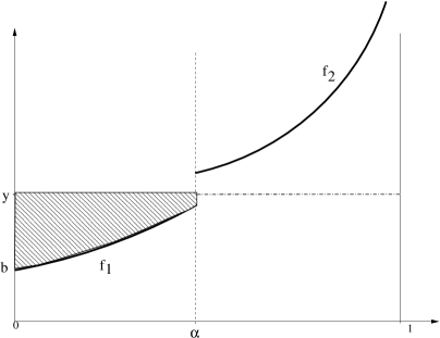
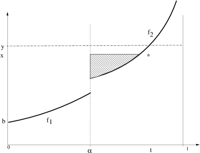
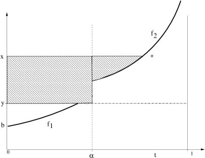
Figure 1(a) provides a graphical description of the stopping rule $\tau$. For $t\leq\alpha$, a decision maker stops if a particle $(t,x)$ with $x\leq y$ and $x\leq f_{1}(t)$ is observed, while for $t>\alpha$, the threshold $f_{2}$ is applied. Figure 1(a) shows one realization of $Y$, where $y<f_{1}(\alpha)$. The decision whether to stop with the first $(t,x)$ such that $x\leq f_{1}(t)$ and $t\leq\alpha$ depends on $y$ only if $t\in(f_{1}^{-1}(y),\alpha]$. Figure 1(b) provides an example where $y>f_{1}(t)$ for all $t\leq\alpha$. In this case, the decision maker stops with the first $(t,x)$, such that $0\leq t\leq\alpha$ and $x\leq f_{1}(t)$, if any such $(t,x)$ exists.

To obtain the risk $\mathbb{E}\left[R(\tau,X)\right]$, we consider the conditional risk $\mathbb{E}\left[R(\tau,X)|Y=y\right]$ and integrate out $y$. To do this, we define

$$F_{1}(t,y) := \int_{0}^{t}\left(f_{1}(s)\wedge y\right)ds\ ,\ \ \ F_{2}(t):=\int_{\alpha}^{t}f_{2}(s)ds\ ,\text{ and }$$ (3)

$$S_{1}(x) := \int_{0}^{x}\left(f_{1}^{-1}(z)\wedge\alpha\right)dz=\alpha x-F_{1}(\alpha,x)\ ,\$$ (4)

where $f_{1}^{-1}(z)$ = 0 for $z<f_{1}(0)$. Furthermore,

$$S_{2}(x) := \int_{0}^{x}\left(f_{2}^{-1}(z)-\alpha\right)dz\ ,\$$ (5)

where $f_{2}^{-1}(z)=\alpha$ for $z<f_{2}(\alpha)$. By the properties of the planar Poisson process the probability that the area bounded by the horizontal line with height $y$ and the graph of $f_{1}$ for the time interval $[0,\alpha]$ is empty is $e^{-S_{1}(y)}$; see the shaded area in Figure 1(b). Hence, the density of $Y$ is

$$\mathbb{P}\left(Y\in dy\right) = \left[\frac{d}{dy}\left(1-e^{-S_{1}(y)}\right)\right]dy=e^{-S_{1}(y)}\left(f_{1}^{-1}(y)\wedge\alpha\right)dy\ .\$$ (6)

By the definition of $Y$, $\mathbb{P}\left(Y\in dy\right)>0$, for $y>f_{1}(0)$ and zero else. Given $\{Y=y\}$, the conditional joint density of $(\tau,X)$ is

$$\mathbb{P}\left((\tau,X)\in(dt,dx)|Y=y\right) = \begin{cases}e^{-F_{1}(t,y)}dt\ dx&0\leq t\leq\alpha,\ \ \ 0\leq x\leq f_{1}(t)\wedge y\ ,\\ e^{-F_{1}(\alpha,y)-F_{2}(t)}dt\ dx&\alpha<t\leq 1,\ \ \ 0\leq x\leq f_{2}(t)\ .\end{cases}$$ (7)

By means of the density (7), we obtain the conditional probability $\mathbb{P}\left(\tau>t|Y=y\right)=e^{-F_{1}(t,y)}$, for $t\leq\alpha$, and $\mathbb{P}\left(\tau>t|Y=y\right)=e^{-F_{1}(\alpha,y)-F_{2}(t)}$, for $\alpha<t\leq 1$. Splitting the time at $\alpha$, the two components of the risk given $Y=y$ are computed as

$$\mathbb{E}\left[R(\tau,X)\mathbf{1}_{(\tau\leq\alpha)}|Y=y\right] = \int_{0}^{\alpha}e^{-F_{1}(t,y)}\left(\int_{0}^{f_{1}(t)\wedge y}\left(1+x(1-t)\right)\ dx\right)\ dt\ \text{ and }$$

$$\mathbb{E}\left[R(\tau,X)\mathbf{1}_{(\tau>\alpha)}|Y=y\right] = \int_{\alpha}^{1}e^{-F_{1}(\alpha,y)-F_{2}(t)}\left[\int_{0}^{f_{2}(t)\wedge y}\left(1+x(1-t)\right)\ dx+\int_{f_{2}(\alpha)}^{f_{2}(t)}S_{2}(x)\ dx\right.$$ (8)

$$+\left.\int_{f_{2}(t)\wedge y}^{f_{2}(t)}\left(2+x(1-t)+(x-y)\alpha\right)\ dx\right]\ dt\ .$$

For $t\leq\alpha$, the integrand of the inner integral describes the conditional expected loss contribution when we stop at $(t,x)$. In this case, the relative rank of $(t,x)$ is $1$ and the conditional expected loss of $(t,x)$ is $1$ plus the expected number of atoms in the south-east of $(t,x)$. That is, $1+x(1-t)$. An example for such a $(t,x)$ is provided by “$*$” in Figure 1(a). For $t\geq\alpha$, we have to account for atoms in the area above the curve $f_{2}(s)$, $\alpha<s\leq t$ and below the level obtained by $x$. In the Figures 1(c) and 1(d) this corresponds to the almost triangular shaded area. Formally, the size of this area is $S_{2}(x)$, where $S_{2}(x)=0$, for $x\leq f_{2}(\alpha)$ and $S_{2}(x)>0$, for $x>f_{2}(\alpha)$. In particular, Figure 1(c) shows $S_{2}(x)$, for some $x>f_{2}(\alpha)$. Figures 1(c) and 1(d) describe two generic cases where a decision maker stops at $(t,x)$ with $t>\alpha$. Figure 1(c) describes the case $y>x$. The loss coming from the past is described by the shaded almost triangular area. The conditional expected loss is $1+x(1-t)+S_{2}(x)$. $1$ accounts for the particle itself and $x(1-t)$ for the expected loss in the future, which is the size of the area in the south-east of the particle $(t,x)$. Next, Figure 1(d) describes the case where $y\leq x$. In this case, the loss coming from the past is described by the shaded almost triangular area and the shaded rectangular area. The conditional expected loss is $2+x(1-t)+S_{2}(x)+(x-y)\alpha$. $2$ accounts for the particle itself and the particle $(t^{\prime},y)$, such that $y$ is the realization of $Y$. In addition, $x(1-t)$ accounts for the expected loss in the future. Last but not least, $F_{1}(t,y)$ and $F_{2}(t)$ measure the size of areas below $f_{1}(s)\wedge y$, where $0\leq s\leq t$, and $f_{2}(s)$, where $\alpha<s\leq t$. $S_{1}(y)$ measures to the difference of the size of the area of the rectangle described by the points $(0,0)$, $(\alpha,0)$, $(\alpha,f_{1}(\alpha)\wedge y)$ and $(0,f_{1}(\alpha)\wedge y)$ and the size of the area below the graph $\{\left(t,f_{1}(t)\wedge y\right):\ 0\leq t\leq\alpha\}$. The shaded area in Figure 1(b) provides an example for this area.

Next, we work with $f_{1}(t)=\frac{b}{1-t}$ and $f_{2}(t)=\frac{c}{1-t}$. For these functions, we were able to obtain the conditional expected losses $\mathbb{E}\left[R(\tau,X)\mathbf{1}_{(\tau\leq\alpha)}|Y=y\right]$ and $\mathbb{E}\left[R(\tau,X)\mathbf{1}_{(\tau>\alpha)}|Y=y\right]$, as well as the expected loss $\mathbb{E}\left[R(\tau,X)\right]=\int_{b}^{\infty}\left(\mathbb{E}\left[R(\tau,X)\mathbf{1}_{(\tau\leq\alpha)}|Y=y\right]+\mathbb{E}\left[R(\tau,X)\mathbf{1}_{(\tau\leq\alpha)}|Y=y\right]\right)e^{-S_{1}(y)}\left(f_{1}^{-1}(y)\wedge\alpha\right)dy$ in closed form by using the Mathematica 8.0 package.

To minimize $\mathbb{E}\left[R(\tau,X)\right]$ the parameters $\alpha$, $b$ and $c$ have to be chosen optimally. By numerical tools we observed that the value of the loss function is approximately minimized with $(\alpha_{*},b_{*},c_{*})=(0.34328,1.82571,2.00000)$. With these parameters we calculated an expected loss of $2.32614$.

Remark 1.

To check the above results we performed various simulation studies. We observe that our rule with $(\alpha_{*},b_{*},c_{*})=(0.34328,1.82571,2.00000)$ dominates the rule of Tamaki, (2004), where $(\alpha_{T},b_{T},c_{T})=(0.42,1.95,1.95)$, as well as the threshold rule presented in Gnedin, (2007), where $(\alpha_{G},b,c_{G})=(0,b,1.9469)$ and $b>0$ is arbitrary, in the mean. For this threshold rule the expected rank is $1+\frac{c_{G}}{2}+\frac{1}{c_{G}^{2}-1}=2.3318$.

At the end of their paper, Assaf and Samuel-Cahn, (1996) mentioned in Remark 6.2 that they tried a rule that would be in retrospect the $n$-period analogue of our rule, but with $b=c$ (as already mentioned, this rule has been investigated by Tamaki, (2004), where a value of $2.33044$, with $\alpha_{T}=0.42$ and $b_{T}=c_{T}=1.95$, has been obtained in closed form). That is, they tried thresholds, where in the beginning fraction of time $\gamma$ the additional condition of stopping only with relative rank $1$ is imposed, and then a threshold rule is used for the remaining time. However, they left the thresholds at $\min\{2/(n-k+1),1\}$, for $k=1,\dots,n$ (these thresholds had been known to be good approximations for thresholds of the optimal threshold rule for large enough $n$).

Assaf and Samuel-Cahn, (1996) reported that “the improvement is however very small, and even with $10,000$ simulations the standard error is too large to determine whether the improvement is real.” Also in our simulation runs (with 50,000 steps), we observed that the standard errors are large compared to the improvements obtained with our rule and the rule of Tamaki, (2004), which also implies that a reliable comparison of rules can hardly be performed by means of a simulation analysis.

In addition, we inserted the parameters $(\alpha_{T},b_{T},c_{T})$ and $(\alpha_{G},b,c_{G})$ into our closed form expression obtained for $\mathbb{E}\left[R(\tau,X)\right]$. For the threshold rule, the difference between the number we get by inserting the corresponding parameters into the expression obtained for $\mathbb{E}\left[R(\tau,X)\right]$ and the number we get by means of $1+\frac{c_{G}}{2}+\frac{1}{c_{G}^{2}-1}$ is smaller than $4\cdot 10^{-8}$. For $(\alpha_{T},b_{T},c_{T})$ we obtained $2.33045$ instead of $2.33044$ derived by Tamaki, (2004). That is, up to a numerical error, the expected losses obtained in Tamaki, (2004) and Gnedin, (2007) can also be replicated by means of the closed form expression in this article.

(a) Stopping Rule $\tau$. $f_{1}=\frac{b}{1-t}$, $f_{2}=\frac{c}{1-t}$.

(b) Area between $y$ and and the graph of $f_{1}(t)$.

(c) Loss components, $y>f_{2}(t)$ is a realizations of $Y$.

(d) Loss components, $y<f_{2}(t)$ is a realiations of $Y$.

Figure 1: The stopping rule $\tau$ and loss components.

Appendix A Mathematica Code

The following pages present the Mathematica code used to obtain the expected loss $\mathbb{E}\left[R(\tau,X)\right]$:

See pages 1-15 of meiersoegner_mathematicadocument.pdf

References

- Assaf and Samuel-Cahn, (1996) Assaf, D. and Samuel-Cahn, E. (1996). The secretary problem: Minimizing the expected rank with i.i.d. random variables. Advances in Applied Probability, 28(3):828–852.
- Bruss, (2005) Bruss, F. T. (2005). What is known about Robbins’ problem? Journal of Applied Probability, 42(1):108–120.
- Bruss and Ferguson, (1993) Bruss, F. T. and Ferguson, T. S. (1993). Minimizing the expected rank with full information. Journal of Applied Probability, 30(3):616–626.
- Bruss and Ferguson, (1996) Bruss, F. T. and Ferguson, T. S. (1996). Half-prophets and Robbins’ problem of minimizing the expected rank. In Lecture Notes in Statistics, pages 1–17. Springer.
- Bruss and Delbaen, (2001) Bruss, T. F. and Delbaen, F. (2001). Optimal rules for the sequential selection of monotone subsequences of maximum expected length. Stochastic Processes and their Applications, 96(2):313–342.
- Bruss and Swan, (2009) Bruss, T. F. and Swan, Y. C. (2009). A continuous-time approach to Robbins’ problem of minimizing the expected rank. Journal of Applied Probability, 46(1):1–18.
- Gnedin and Iksanov, (2011) Gnedin, A. and Iksanov, A. (2011). Moments of random sums and Robbins’ problem of optimal stopping. Journal of Applied Probability, 48(4):1197–1199.
- Gnedin, (1996) Gnedin, A. V. (1996). On the full-information best-choice problem. Journal of Applied Probability, 33:678–687.
- Gnedin, (2004) Gnedin, A. V. (2004). Best choice from the planar poisson process. Stoch. Proc. Appl, pages 317–354.
- Gnedin, (2007) Gnedin, A. V. (2007). Optimal stopping with rank-dependent loss. Journal of Applied Probability, 44:996–1011.
- Swan, (2011) Swan, Y. (2011). A contribution to the study of Robbins’ problem. Memoire de l’Acadamie Royale des Siences, des Lettres et des Beaux-Arts.
- Tamaki, (2004) Tamaki, M. (2004). The PPP approach to Robbins’ problem of minimizing the expected rank. RIMS Kokyuroku, 1383:130–139.