Quantum-enhanced microscopy with binary-outcome photon counting

Abstract

Polarized light microscopy using path-entangled $N$-photon states (i.e., the N00N states) has been demonstrated to surpass the shot-noise limit at very low light illumination. However, the microscopy images suffer from divergence of phase sensitivity, which inevitably reduces the image quality. Here, we show that due to experimental imperfections, such a singularity also takes place in the microscopy that uses twin-Fock states of light for illumination. We propose two schemes to completely eliminate this singularity: (i) locking the phase shift sensed by the beams at the optimal working point, by using a spatially dependent offset phase; (ii) a combination of two binary-outcome photon counting measurements, one with a fixed offset phase and the other without any offset phase. Our observations remain valid for any kind of binary-outcome measurement and may open the way for quantum-enhanced microscopy with high $N$ photon states.

I Introduction

Light microscopy at low light illumination is desirable to avoid damaging the specimen (e.g., the biological samples) Brida ; Taylor ; Lemos ; Ono ; Israel . At very low light level, it might be more efficient to use nonclassical light for illumination, such as twin beams from a parametric down-converted light Brida and amplitude squeezed light Taylor . Recently, polarized light microscopy using path-entangled $N$-photon states (i.e., the N00N states) $\sim(|N,0\rangle+|0,N\rangle)$ was demonstrated to enlarge the contribution of each photon to the image contrast Ono ; Israel , where $|m,n\rangle\equiv|m\rangle_{H}\otimes|n\rangle_{V}$ denotes the product of photon Fock states of two orthogonal polarization modes $H$ and $V$. From binary-outcome photon counting Ono ; Israel , it was found that the birefringence phase shift of a sample $\phi(x,y)$ can be estimated beyond the shot-noise limit, i.e., the phase sensitivity $\delta\phi(x,y)<1/\sqrt{N}$. However, the phase sensitivity diverges at certain values of phase shift, which in turn reduces the quality of microscopy images Israel .

Compared with the N00N states, the twin-Fock states $|n,n\rangle$ are easier to prepare and more robust against photon loss HB ; FWSun ; GYXiang10 ; Xiang . Recently, it was shown that the visibility of the 6-photon count rate could reach $\sim 94\%$ Xiang , significantly better than that of a five-photon N00N state Afek . In addition, the achievable phase sensitivity can surpass that of the N00N states with a binary-outcome photon counting Xiang . Similar to Ref. Israel , however, we will show that quantum-enhanced microscopy illuminated by the twin-Fock state of the light (or any finite-$N$ input state) also suffers from the divergence of the phase sensitivity. To remedy this problem, we propose a scheme to lock the phase shift sensed by the beams at the optimal working point using three estimators nearby, as illustrated schematically by Fig. 1(a). We further show that a combination of two binary-outcome photon counting, one with a fixed offset phase and the other without any offset phase, also works to remove the singularity. Our results can be generalized to any kind of binary-outcome measurement that has been widely adopted in quantum metrology Bollinger ; Dowling ; Gerry ; Cohen ; Brivio ; Distante ; XMFeng , and recently in quantum-enhanced microscopy Ono ; Israel .

II Binary-outcome photon counting using twin-Fock states of light

As illustrated schematically in Fig. 1(a), we consider a quantum-enhanced microscopy illuminated by the twin-Fock states of light $|n,n\rangle$ HB ; FWSun ; GYXiang10 ; Xiang , with the number of photons $N=2n$. The microscopy images can be constructed from the coincidence photon counting at the output ports Ono ; Israel . Theoretically, the conditional probability for detecting $n_{1}$ photons in the $H$ polarization mode and $n_{2}$ photons in the $V$ polarization mode is given by

$$P(n_{1},n_{2}|\theta)=\left|\langle n_{1},n_{2}|e^{-i[\varphi+\phi(x,y)]J_{y}}|n,n\rangle\right|^{2},$$ (1)

where $\varphi$ is a controllable offset phase, $\phi(x,y)$ is the spatially dependent phase shift caused by the birefringence of the polarized beams inside the sample Israel , and $\theta(x,y)\equiv\varphi+\phi(x,y)$. The phase accumulation $\exp(-i\theta J_{y})$ can be implemented with a polarization Mach-Zehnder interferometer Yurke ; Sanders95 ; Kim98 , corresponding to a rotation around the $y$-component of the Stokes vector $\boldsymbol{J}=(a_{H}^{\dagger},a_{V}^{\dagger})\boldsymbol{\sigma}(a_{H},a_{V})^{T}/2$, where $a_{H}$ ($a_{V}$) is the annihilation operator of the polarization mode $H$ ($V$), and $\boldsymbol{\sigma}$ denotes the Pauli operator.

The photon detection event $n_{1}=n_{2}=n$ is of interest FWSun ; GYXiang10 ; Xiang and is denoted as the outcome “$+$”. This is indeed a projection measurement, or equivalently, a binary-outcome measurement (see Appendix A). The output signal is $\langle\mu(\theta)\rangle\equiv\langle\psi(\theta)|\mu|\psi(\theta)\rangle=P(n,n|\theta)$, where $\mu=|n,n\rangle\langle n,n|$ and $|\psi(\theta)\rangle=\exp(-i\theta J_{y})|\psi_{\mathrm{in}}\rangle$. For each given phase shift $\theta\in(-\pi,\pi)$, after $\mathcal{N}$ binary-outcome measurements, the signal is measured by the count rate $P(n,n|\theta)\simeq\mathcal{N}_{+}/\mathcal{N}$, where $\mathcal{N}_{+}$ is the occurrence number of the event $n_{1}=n_{2}=n$. In Fig. 1(c), we show the statistical average of $\mathcal{N}_{+}/\mathcal{N}$ and its standard deviation (the circles and the bars) obtained from numerical simulation: first we generate $\mathcal{N}$ random numbers $\{\xi_{1},\xi_{2},...,\xi_{\mathcal{N}}\}$ Pezze&Smerzi uniformly distributed within $[0,1]$, then we obtain the occurrence number $\mathcal{N}_{+}$ as the number of counts for $\xi$ to lie within the interval $[0,P(n,n|\theta)]$. Here, to take the experimental imperfections into account, we have replaced $P(n,n|\theta)$ with $a_{0}P(n,n|\theta)+b_{0}$, with $a_{0}$ and $b_{0}$ related to the imperfect visibility and reduced peak height at the phase origin, respectively (see Appendix B). As depicted in Fig. 1(c), the averaged signal, fitted by $P_{\mathrm{fit}}(n,n|\theta)$, show multifold oscillations and the first dark fringe appears at $\theta_{\mathrm{dark}}\simeq\pi/2$, $\arccos(\sqrt{1/3})$, and $\arctan(\sqrt{2/3})$, from the top to the bottom.

Figure 1: (a) Polarized light microscopy with a feedback offset phase. (b) Quasi-probability distributions of the input $|n,n\rangle$ and the output $\exp(-i\theta J_{y})|n,n\rangle$ on the Poincaré sphere, where $\theta=\varphi+\phi(x,y)$. (c) Statistical average of the count rate (red circles) and its standard deviation (bars) from $\mathcal{N}=100$ measurements and $20$ repetitions. (d) Phase uncertainty of the maximum likelihood estimator (red circles) and the phase sensitivity (blue solid) using $P_{\mathrm{fit}}(n,n|\theta)$. The red dashed line: the sensitivity with the exact $P(n,n|\theta)$. Horizontal grid lines: shot-noise limit $1/\sqrt{N}$ and $\delta\theta_{\mathrm{QCRB}}$ for $N=2n=2$, $4$, $6$.

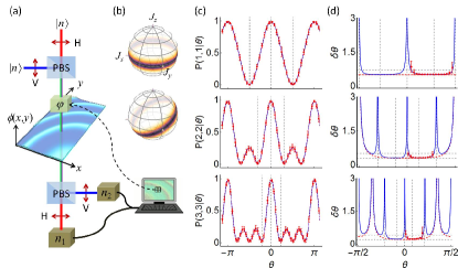
The microscopy images can be reconstructed from the inversion phase estimator Israel , which is a solution of the equation $P(n,n|\theta)=\mathcal{N}_{+}/\mathcal{N}$ (see Appendix A). To avoid the phase ambiguity Pezze ; Higgins ; Berry , we assume that true value of the phase shift lies within a monotonic regime of $P(n,n|\theta)$, e.g., $\theta\in(0,\theta_{\mathrm{dark}})$. The image quality is determined by the phase uncertainty $\delta\theta=\Delta\mu/|\partial\langle\mu(\theta)\rangle/\partial\theta|=1/\sqrt{F(\theta)}$, where, for a single-shot measurement, the fluctuations of signal $(\Delta\mu)^{2}\equiv\langle\mu^{2}\rangle-\langle\mu\rangle^{2}=P(n,n|\theta)[1-P(n,n|\theta)]$ and $F(\theta)$ is the classical Fisher information of the binary-outcome photon counting measurements (see Appendix A). In Fig. 1(d), we plot the phase sensitivity as a function of $\theta$, using the exact (fitted) expression of $P(n,n|\theta)$. For the exact cases (the red dashed lines), the sensitivity reaches minimum at $\theta=0$ FWSun . Due to the experimental imperfections, however, the best sensitivity occurs at $\theta_{\min}\simeq 0.88$, $0.37$, and $0.26$ ($\sim 15^{\circ}$ Xiang ), from the top to the bottom, as depicted by the blue solid lines of Fig. 1(d).

At the optimal working point $\theta_{\min}$, the sensitivity can surpass the shot-noise limit by an enhancement factor $\eta=1/(\sqrt{N}\delta\theta_{\min})\simeq 1.39$ (for $N=2$), $1.61$ ($N=4$), and $1.85$ ($N=6$). Theoretically, the enhancement factor can be predicted by calculating the quantum Fisher information of a phase-encoded state $\exp(-i\theta G)|\psi_{\mathrm{in}}\rangle$ Helstrom ; Braunstein ; Giovannetti , where $G$ is a hermitian operator that encodes a phase shift on the input state $|\psi_{\mathrm{in}}\rangle$. The optimal choice of $G$ is fully determined by quantum correlation of the input state Kitagawa ; Wineland ; Ma ; Toth ; Lucke . For a twin-Fock state, the quasi-probability distribution spreads along the equator of the Poincaré sphere; see Fig. 1(b). This observation suggests that the phase generator can take the form $G=J_{x}\cos\alpha+J_{y}\sin\alpha$ for arbitrary $\alpha$ ($=\pi/2$ in Eq. (1)), which results in the quantum Fisher information $F_{Q}=N(N+2)/2$ and hence the quantum Cramér-Rao bound $\delta\theta_{\mathrm{QCRB}}=1/\sqrt{F_{Q}}\simeq\sqrt{2}/N$. Therefore, the enhancement factor is given by $\eta=1/(\sqrt{N}\delta\theta_{\mathrm{QCRB}})=\sqrt{(N+2)/2}$.

The sensitivity diverges at certain values of $\theta$ (e.g., $\theta=0$, $\pm\theta_{\mathrm{dark}}$). This is because at those points, the slope of the signal $\partial\langle\mu(\theta)\rangle/\partial\theta=0$, but $\Delta\mu\neq 0$, so that $\delta\theta\rightarrow\infty$ (see also Appendix B). Such a singularity could take place for any finite-$N$ input state, e.g., a single-photon state $|1,0\rangle$ and the multi-photon N00N states Israel . For a general binary-outcome measurement, we show that the inversion estimator is indeed the same as the asymptotically optimal maximum likelihood estimator (MLE) Fisher , so the same divergence also occurs for the MLE (see Appendix A). This problem can not be completely avoided even when all the $(N+1)$ outcomes are taken into account.

III Simulated microscopy images

To reconstruct the microscopy images, one first calibrates the interferometer (with no sample present, as done in Ref Israel ) to obtain the averaged signal $P_{\mathrm{fit}}(+|\theta)$ as a function of the phase shift $\theta$. Next, at each spatial point of the sample, one performs the binary-outcome measurements for $\mathcal{N}$ times to record the occurrence frequency for the detection event of interest, and then inverts the averaged signal $P_{\mathrm{fit}}(+|\theta)=\mathcal{N}_{+}(x,y)/\mathcal{N}$ to obtain the inversion estimator $\theta_{\mathrm{est}}(x,y)$. If an offset phase $\varphi$ is applied before the sample, then the estimator becomes $\phi_{\mathrm{est}}(x,y)=\theta_{\mathrm{est}}(x,y)-\varphi$ Israel , where the offset phase $\varphi$ is chosen such that the total phase shift $\theta=\varphi+\phi(x,y)\in[\theta_{\min},\theta_{\mathrm{dark}})$ senrange .

The birefringence phase shift used here is $\phi(x,y)=0.1+0.437\cos^{6}[2(x-\pi/2)^{2}+y^{2}]\in(0.1,0.537]$, which can be discretized into pixels $(i,j)$, with $i,j=0,1,2,\cdots$. At each pixel, performing the photon-counting measurements for $\mathcal{N}$ times and inverting the signal, one can obtain the inversion estimator $\phi_{\mathrm{est}}(i,j)=\theta_{\mathrm{est}}(i,j)-\varphi$, where $\theta_{\mathrm{est}}$ is a solution to $P_{\mathrm{fit}}(+|\theta)=\mathcal{N}_{+}(i,j)/\mathcal{N}$. For each input twin-Fock state, $P_{\mathrm{fit}}(+|\theta)$ has been obtained from the calibration of the interferometer (see the blue solid lines of Fig. 1(c), and also Appendix B), and $\mathcal{N}_{+}(i,j)$ denotes the occurrence number of the outcome “$+$” at the pixel $(i,j)$.

To simulate the microscopy illuminated by a classical light, we consider a single-photon state $|1,0\rangle$ as the input and treat the detection event $n_{1}=1$ and $n_{2}=0$ as the outcome “$+$”, which occurs with probability $P(+|\theta)=\cos^{2}(\theta/2)$. Photon counting over the other outcome gives $P(-|\theta)=\sin^{2}(\theta/2)$, as demonstrated recently by Israel et al Israel . Both of them exhibit the same phase dependence as that of a coherent-state input light $|\alpha\rangle\otimes|0\rangle$ Distante ; XMFeng .

Figure 2 shows the simulated microscopy images using the inversion estimator $\phi_{\mathrm{est}}(i,j)$ for the input twin-Fock states $|n,n\rangle$ with $n=N/2=1,2,3$, and that of the single-photon state $|1,0\rangle$. To keep exactly $600$ photons at each pixel, we use the number of measurements $\mathcal{N}=600$ (a), $300$ (b), $150$ (c), and $100$ (d). From Fig. 2(d), one can note that for the $6$-photon state $|3,3\rangle$, the simulated microscopy image is less accurate at some spatial points (see the speckles). This is because the sensed phase shift $\theta=\varphi+\phi(i,j)\sim\theta_{\mathrm{dark}}$, at which the phase sensitivity diverges. Similar phenomenon takes place for the triphoton N00N state Israel , and also for any finite-$N$ photon state.

Figure 2: Simulated microscopy images ($30\times 60$ pixels) reconstructed from the phase estimator $\phi_{\mathrm{est}}(i,j)$ for the single-photon state (a), and the twin-Fock states with $N=2n=2$ (b), $4$ (c), and $6$ (d). The number of photons at each pixel $\mathcal{N}\times N=600$. Within the area enclosed by the green solid lines, the phase shift sensed by the beams is almost optimal, and numerical simulation of the local standard deviation from $20$ repetitions gives $\mathrm{LSD}_{|1,0\rangle}=0.0413$, $\mathrm{LSD}_{|1,1\rangle}=0.0297$, $\mathrm{LSD}_{|2,2\rangle}=0.0253$, and $\mathrm{LSD}_{|3,3\rangle}=0.022$, indicating $\mathrm{LSD}_{|1,0\rangle}/\mathrm{LSD}_{|n,n\rangle}\approx\sqrt{(N+2)/2}$.

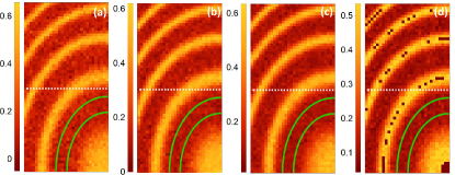
The image quality is improved with the quantum source of the light as long as the sensed phase shift is far from the singular points Israel . To quantify such a improvement, we calculate standard deviation of $\phi_{\mathrm{est}}(i,j)$ within a local area enclosed by the green solid lines of Fig. 2, as denoted by $\mathrm{LSD}_{|\psi_{\mathrm{in}}\rangle}$. Similar to Ref. Israel , we focus on the relative noise $\mathrm{LSD}_{|1,0\rangle}/\mathrm{LSD}_{|n,n\rangle}$, which gives a measure of the improvement in the image quality beyond the classical illumination. From each image of Fig. 2, one can extract $\mathrm{LSD}_{|\psi_{\mathrm{in}}\rangle}$ and hence the relative noise. Taking $20$ pictures for each input state, we obtain $\mathrm{LSD}_{|1,0\rangle}/\mathrm{LSD}_{|n,n\rangle}=1.39$ (for $n=N/2=1$), $1.63$ ($n=2$), and $1.88$ ($n=3$), in agreement with the enhancement factor $\eta$.

IV Phase locking to the optimal working point

Due to the divergence of the phase sensitivity, the sensing range of the quantum-enhance microscopy becomes narrow, especially when a higher-$N$ nonclassical state is injected. In order to remedy this problem, we propose a scheme to control the offset phase at each spatial point of the sample according to three estimators nearby, as illustrated schematically by Fig. 1(a).

The basic idea is to insert a spatially dependent offset phase $\varphi(i,j)$, such that the total phase sensed by the beams is close to the optimal working point: $\theta(i,j)\equiv\varphi(i,j)+\phi(i,j)\sim\theta_{\min}$. To determine the offset phase, we need some prior information to the unknown phase $\phi(i,j)$ before the measurements. Quantum measurements with adaptive feedback maximizes the information gain in subsequent measurements and have been experimentally shown to be a powerful technique to achieve the precision beyond the shot-noise limit GYXiang10 ; Higgins . However, application of the existing feedback-based phase estimation (see e.g., Ref. Berry2000 ) in the microscopy is generally very challenging. For our binary-outcome measurements, a global feedback strategy for $\mathcal{N}_{\mathrm{tot}}$ measurements requires solving a set of nonlinear equations with $2^{\mathcal{N}_{\mathrm{tot}}+1}-1$ unknown variables Berry2000 . Recently, Hentschel and Sanders Sanders proposed an approximate scheme that reduces the number of unknown variables to $\sim O(\mathcal{N}_{\mathrm{tot}})$. Here we are interested in estimating the values of the phases at all the pixels of the sample, which typically requires $\mathcal{N}_{\mathrm{tot}}=\mathcal{N}\times N_{\mathrm{pixels}}\sim 10^{6}$, where $N_{\mathrm{pixels}}$ denotes total number of pixels. In this case, even the approximate strategy becomes formidable.

We present a simple but effective scheme that adjusts the offset phase after every $\mathcal{N}$ measurements per pixel. Specially, we first estimate the true value of phase shift at the pixel $(0,0)$, e.g., $\phi_{\mathrm{est}}(0,0)\simeq 0.1\mathrm{rad}$. From the starting point, we can obtain all the estimators by adjusting the offset phase as illustrated in Fig. 3(a) and (b). For instance, to estimate $\phi(1,0)$, we adjust the offset phase as $\varphi(1,0)=$ $\theta_{\min}-\phi_{\mathrm{est}}(0,0)$, which ensures the phase locking to the optimal working point $\theta(1,0)=\varphi(1,0)+\phi(1,0)\simeq\theta_{\min}$, provided $\phi(1,0)\simeq\phi_{\mathrm{est}}(0,0)$. With this offset phase, one performs $\mathcal{N}$ measurements at the pixel $(1,0)$ to obtain a local phase estimator $\phi_{\mathrm{est}}(1,0)=\theta_{\mathrm{est}}-\varphi(1,0)$, where $\theta_{\mathrm{est}}$ is a solution to $P_{\mathrm{fit}}(+|\theta)=\mathcal{N}_{+}(1,0)/\mathcal{N}$. Similarly, one can obtain the estimator $\phi_{\mathrm{est}}(0,1)$. To estimate $\phi(1,1)$, we use the three estimators in a rectangle and adjust the offset phase to $\varphi(1,1)=\theta_{\min}-[\phi_{\mathrm{est}}(0,1)+\phi_{\mathrm{est}}(0,0)+\phi_{\mathrm{est}}(1,0)]/3$, which helps to lock $\theta(1,1)=\varphi(1,1)+\phi(1,1)$ at the pixel $(1,1)$ to the optimal working point $\theta_{\min}$. Repeating the above procedures, one can measure the phase of all the pixels over the entire sample.

Figure 3: Two steps of the phase locking (a) and (b), the simulated microscopy image for the input 6-photon state $|3,3\rangle$ (c), and the true value of phase shift (d). In (a), the offset phase is tuned as $\varphi(i,0)=\theta_{\min}-\phi_{\mathrm{est}}(i-1,0)$, and $\varphi(0,j)=\theta_{\min}-\phi_{\mathrm{est}}(0,j-1)$; in (b), it becomes $\varphi(i,j)=\theta_{\min}-[\phi_{\mathrm{est}}(i-1,j)+\phi_{\mathrm{est}}(i,j-1)+\phi_{\mathrm{est}}(i-1,j-1)]/3$. In (c) $\mathcal{N}=100$ to keep exactly $600$ photons at each pixel. The inset in (d): the simulated estimators at the pixel $y=30$ as a function of $x$ (blue solid) and that of the true value of phase shift (red dashed).

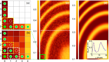
In Fig. 3(c), we show the microscopy image for the 6-photon state $|3,3\rangle$ using the phase locking method. The main advantage of this method is that the singular points (i.e., the speckles) disappear. Furthermore, compared with previous adaptive feedback schemes GYXiang10 ; Berry2000 ; Sanders that adjusts a controllable phase after each single measurement, our scheme updates the offset phase every $\mathcal{N}$ measurements. This costs much less computational resources, while it can still improve the image quality significantly. The overall quality of the image can be quantified by the root-mean-square error, i.e., $\mathrm{RMSE}=\sqrt{\sum_{i,j}[\phi_{\mathrm{est}}(i,j)-\phi(i,j)]^{2}/N_{\mathrm{pixels}}}$, which approaches the optimal value of the standard deviation $\mathrm{LSD}_{|3,3\rangle}=0.022$, as depicted in Fig. 2(d). This observation implies that at most of the pixels, the phase shift sensed by the beams is optimal.

V Combination of two binary-outcome measurements

The phase locking scheme requires control of the feedback phase after every $\mathcal{N}$ measurements at each pixel. To further reduce the cost, one can use a fixed offset phase $\varphi$ (as implemented experimentally in Ref. Israel ) and then perform two sequences of binary-outcome photon counting measurements: one sequence with the offset phase $\varphi$ and the other sequence without any offset phase. Then we combine all the measurement results to obtain the MLE and hence the microscopy images, i.e., $\phi_{\mathrm{mle}}(i,j)$.

Following Ref. Israel , let us begin with the calibration the interferometer using different known values of phase shift $\phi$ and a fixed offset phase $\varphi$ for each input state. Performing $\mathcal{N}_{1}$ measurements without the offset phase, one can obtain the occurrence number $\mathcal{N}_{1}^{(+)}$ for the outcome $n_{1}=n_{2}=n$. In the presence of the offset phase, one performs another $\mathcal{N}_{2}$ measurements over the output state $\exp[-i(\phi+\varphi)J_{y}]|n,n\rangle$ to obtain the occurrence number $\mathcal{N}_{2}^{(+)}$. In the upper panel of Fig. 4, we plot the averaged count rates $\mathcal{N}_{1}^{(+)}/\mathcal{N}_{1}$ and $\mathcal{N}_{2}^{(+)}/\mathcal{N}_{2}$ (the circles) as functions of $\phi$ and fit them as $P_{\mathrm{fit}}(+|\phi)$ (the blue solid) and $P_{\mathrm{fit}}(+|\varphi+\phi)$ (the red dashed), respectively.

Figure 4: Simulated count rates (a)-(c) and uncertainty of the MLE (d)-(f) for $\varphi=-0.3\times\theta_{\mathrm{dark}}$ and $\mathcal{N}_{1}=\mathcal{N}_{2}=\mathcal{N}/2$, where $N\times\mathcal{N}=1200$ is fixed for the input states $|1,1\rangle$ (left), $|2,2\rangle$ (middle), and $|3,3\rangle$ (right). Red dashed lines in (d)-(f): the phase sensitivity $1/\sqrt{F(\phi)}$, with the locations of $\theta_{\mathrm{dark}}$ indicated by the vertical lines; Blue solid lines: the sensitivity with the total Fisher information (see text). The inset: statistical average of $\phi_{\mathrm{mle}}$ as a function of $\phi$ for $20$ repetitions.

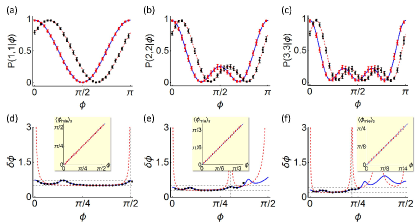
Next, we perform the above binary-outcome photon counting at each pixel of the sample for totally $\mathcal{N}$ ($=\mathcal{N}_{1}+\mathcal{N}_{2}$) measurements to retrieve $\phi_{\mathrm{mle}}$ that maximizes the likelihood function:

$$\mathcal{L}(\phi)\!\! \varpropto \!\!\left[P_{\mathrm{fit}}\left(+|\varphi+\phi\right)\right]^{\mathcal{N}_{2}^{(+)}}\left[1-P_{\mathrm{fit}}\left(+|\varphi+\phi\right)\right]^{\mathcal{N}_{2}-\mathcal{N}_{2}^{(+)}}$$ (2)

$$\times\left[P_{\mathrm{fit}}\left(+|\phi\right)\right]^{\mathcal{N}_{1}^{(+)}}\left[1-P_{\mathrm{fit}}\left(+|\phi\right)\right]^{\mathcal{N}_{1}-\mathcal{N}_{1}^{(+)}},$$

where the occurrence numbers $\mathcal{N}_{1}^{(+)}$ and $\mathcal{N}_{2}^{(+)}$ are spatially dependent, containing phase information of the sample. At each pixel $(i,j)$, the phase estimator $\phi_{\mathrm{mle}}$ and its uncertainty $\sigma$ can be obtained by numerically finding the peak of the likelihood function and the $68.3\%$ confidence interval around the peak Pezze&Smerzi . The inset of Figs. 4(d)-(f) shows statistical average of the estimator $\langle\phi_{\mathrm{mle}}\rangle_{s}=\phi$, indicating that $\phi_{\mathrm{mle}}$ is unbiased for $\phi\in(0,\theta_{\mathrm{dark}})$. Interestingly, we find that the averaged phase uncertainty per measurement $\sqrt{\mathcal{N}}\langle\sigma\rangle_{s}$ (the circles) follows the lower bound of the phase sensitivity $\delta\phi\!=\!\sqrt{\mathcal{N}}/\sqrt{F_{\mathrm{tot}}(\phi)}$ (the blue solid lines), where $F_{\mathrm{tot}}(\phi)=\mathcal{N}_{1}F(\phi)+\mathcal{N}_{2}F(\phi+\varphi)$ is the total Fisher information of all the two sequences of binary-outcome measurements and $F(\phi)$ is the Fisher information of a single sequence of the measurements (see Appendix A, Eq. (6)). Obviously, the singularity of $\delta\phi$ can be completely eliminated by a suitable choice of the offset phase $\varphi$ (which maximizes the total Fisher information), in sharp contrast to the previous result Israel ; senrange .

In Fig. 4, we show that with a fixed offset phase $\varphi=-0.3\times\theta_{\mathrm{dark}}$ for each input twin-Fock state, the unbiased estimator $\phi_{\mathrm{mle}}$ does not show any singularity and its uncertainty can surpass the shot-noise limit as $\phi$ increases up to $\sim\theta_{\mathrm{dark}}$. It is therefore useful for estimating the phase information of a sample at the sub-shot-noise limit through $\phi_{\mathrm{mle}}(i,j)$.

VI Conclusion

In summary, we have investigated theoretically the binary-outcome photon counting and its potential applications in quantum-enhanced microscopy using the input twin-Fock states of light. Our results show that the inversion estimator is the same to the asymptotically optimal maximum likelihood estimator. Both estimators may suffer from a divergent uncertainty that reduces the quality of the microscopy images. To remedy this problem, we propose a simple method to lock the phase shift sensed by the beams at the optimal working point with a spatially dependent offset phase. The overall image quality outperforms the case of classical light illumination by a factor $\sim\sqrt{(N+2)/2}$. We further show that a combination of two sequences of binary-outcome photon counting measurements, one sequence with a fixed offset phase and the other sequence without any offset phase, also works to remove the singularity. Our results remain valid for any kind of binary-outcome measurement and pave the way for realistic implementations of quantum-enhanced microscopy that uses high-$N$ nonclassical states of the light.

Appendix A Phase estimators for a general binary-outcome measurement

In the following, we introduce the concept of binary-outcome measurement and present the details of our numerical simulations.

Binary-outcome measurements have been widely adopted in quantum metrology Bollinger ; Dowling ; Gerry ; Cohen ; Brivio ; Distante ; XMFeng , and recently in quantum-enhanced microscopy Ono ; Israel . As the simplest measurement scheme, the output signal can be expressed as

$$\langle\mu(\theta)\rangle=\sum_{i=\pm}\mu_{i}P\left(i|\theta\right)\approx\sum_{i=\pm}\mu_{i}\frac{\mathcal{N}_{i}}{\mathcal{N}},$$ (3)

where $\mathcal{N}_{\pm}/\mathcal{N}$ denotes the occurrence frequency of the outcome $\mu_{\pm}$, measured by the normalized coincidence rate with a finite number of photon counts $\mathcal{N}=\mathcal{N}_{+}+\mathcal{N}_{-}$. For the input twin-Fock states $|n,n\rangle$ FWSun ; GYXiang10 ; Xiang , the specific detection event $n_{1}=n_{2}=n$ is of interest and can be treated as the outcome “$+$” and the others as “$-$”, with the conditional probability $P(+|\theta)\equiv P(n,n|\theta)$ and hence $P(-|\theta)=1-P(+|\theta)$. Taking $\mu_{+}=+1$ and $\mu_{-}=0$, the signal becomes $\langle\mu(\theta)\rangle=P(+|\theta)=P(n,n|\theta)$, as expected. Similarly, the parity detection gives two outcome $\pm 1$, according to even or odd number of photons being detected at one port of the interferometer Bollinger ; Dowling ; Gerry ; Cohen . Recently, quantum-enhanced microscopy with a two-photon N00N state has been demonstrated by counting odd number of photons Ono . For a measurement with continuous-variable outcome, one can also realize a binary-outcome measurement by dividing the date into two bins Distante . These cases are indeed binary-outcome measurement XMFeng .

For any kind of binary-outcome measurement, the inversion estimator $\theta_{\mathrm{est}}$ can be obtained by inverting the averaged signal, which is indeed a solution of Eq. (3), or equivalently $P(+|\theta)=\mathcal{N}_{+}/\mathcal{N}$, independently from the measured values $\mu_{\pm}$. According to the error propagation, the uncertainty of $\theta_{\mathrm{est}}$ depends on the fluctuations of signal $\Delta\mu=(\mu_{+}-\mu_{-})\Delta\mathcal{N}_{+}/\mathcal{N}$, with $\Delta\mathcal{N}_{+}=\sqrt{\mathcal{N}P(+|\theta)P(-|\theta)}$ being standard deviation of a binomial distribution:

$$\mathcal{L}(\theta;\mathcal{N}_{+})=\binom{\mathcal{N}}{\mathcal{N}_{+}}\left[P\left(+|\theta\right)\right]^{\mathcal{N}_{+}}\left[P\left(-|\theta\right)\right]^{\mathcal{N}_{-}},$$ (4)

where $\binom{n}{k}$ is the binomial coefficient, $P(+|\theta)+P(-|\theta)=1$, and hence $\sum_{\mathcal{N}_{+}}\mathcal{L}(\theta;\mathcal{N}_{+})=[P(+|\theta)+P(-|\theta)]^{\mathcal{N}}=1$. On the other hand, from Eq. (3), we obtain the slope of signal $\partial\langle\mu(\theta)\rangle/\partial\theta=(\mu_{+}-\mu_{-})\partial P(+|\theta)/\partial\theta$, which, together with $\Delta\mu$, gives the phase uncertainty

$$\delta\theta=\frac{\Delta\mu}{\left|\partial\langle\mu(\theta)\rangle/\partial\theta\right|}=\frac{\sqrt{P\left(+|\theta\right)P\left(-|\theta\right)}}{\sqrt{\mathcal{N}}\left|\partial P\left(+|\theta\right)/\partial\theta\right|}=\frac{1}{\sqrt{\mathcal{N}F(\theta)}},$$ (5)

where, for a single-shot measurement, the classical Fisher information is given by

$$F(\theta)=\sum_{i=\pm}\frac{1}{P\left(i|\theta\right)}\left[\frac{\partial P\left(i|\theta\right)}{\partial\theta}\right]^{2}.$$ (6)

Our above results indicate that for any binary-outcome measurements with $\mathcal{N}\gg 1$, the simplest data processing based on inverting the averaged signal always saturates the Cramér-Rao lower bound XMFeng . This is somewhat counter intuitive since, according to Fisher’s theorem Fisher , this bound is saturable by maximum likelihood estimator (MLE) as the number of measurements $\mathcal{N}\gg 1$. To understand it, we further investigate the MLE by finding a value of $\theta$ that maximizes Eq. (4); Hereinafter, denoted by $\theta_{\mathrm{mle}}$. When $\mathcal{N}_{\pm}\sim O(\mathcal{N})\gg 1$, the binomial distribution of $\mathcal{L}(\theta;\mathcal{N}_{+})$ becomes normal

$$\mathcal{L}(\theta;\mathcal{N}_{+})\varpropto\exp\left(-\frac{\left[\mathcal{N}_{+}-\mathcal{N}P\left(+|\theta\right)\right]^{2}}{2(\Delta\mathcal{N}_{+})^{2}}\right),$$ (7)

which indicates that the MLE $\theta_{\mathrm{mle}}$ also satisfy the equation $P(+|\theta)=\mathcal{N}_{+}/\mathcal{N}$, the same to that of $\theta_{\mathrm{est}}$.

The phase estimator $\theta_{\mathrm{mle}}$ and its uncertainty can be obtained by maximizing Eq. (4). To avoid the phase ambiguity Pezze ; Higgins ; Berry , we introduce prior knowledge about the true value of $\theta$ by assuming the prior probability $P(\theta)=1$ for $\theta\in(0,\theta_{\mathrm{dark}})$, and $0$ outside, where $\theta_{\mathrm{dark}}$ denotes the location of the first dark fringe; see the vertical dashed lines in Fig. 1(c). Next, we fit the phase distribution as a Gaussian around its peak Pezze&Smerzi , i.e.,

$$\mathcal{P}(\theta|\mathcal{N}_{+})=CP(\theta)\mathcal{L}(\theta;\mathcal{N}_{+})\propto\exp\left[-\frac{(\theta-\theta_{\mathrm{mle}})^{2}}{2\sigma^{2}}\right],$$

where $C$ is a normalized factor, and $\sigma$ is $68.3\%$ confidence interval of the Gaussian around $\theta_{\mathrm{mle}}$, given by

$$\sigma\simeq\sqrt{\frac{C}{|\partial^{2}\mathcal{P}(\theta|\mathcal{N}_{+})/\partial\theta^{2}|_{\theta=\theta_{\mathrm{mle}}}}}.$$ (8)

The above results remain valid for any input state of the probes and is independent from any specific form of the noise. For the input twin-Fock states, the averaged phase uncertainty of the MLE, i.e., $\sqrt{\mathcal{N}}\langle\sigma\rangle_{s}$ (the circles of Fig. 1(d)), shows a good agreement with the sensitivity per measurement $1/\sqrt{F(\theta)}$ (the blue solid line), where $\langle(...)\rangle_{s}\equiv\sum_{i=1}^{M}(...)_{i}/M$ denotes the statistical average for $M$ repetition of measurements.

Appendix B Numerical simulations

We consider a single-photon state $|1,0\rangle$ as the input to simulate the microscopy with a classical illumination Ono ; Israel . It is easy to obtain the conditional probability for detecting a single photon in the horizontal polarization mode and vacuum in the vertical polarization mode, i.e., $P(1,0|\theta)=|\langle 1,0|\exp(-i\theta J_{y})|1,0\rangle|^{2}=\cos^{2}(\theta/2)$. If we treat the detection event $n_{1}=1$ and $n_{2}=0$ as the outcome “$+$”, and the others as “$-$”, then this is indeed a binary-outcome photon counting measurement, with the output signal $\langle\mu(\theta)\rangle=P(+|\theta)=\cos^{2}(\theta/2)$. From Eq. (5), we immediately obtain the phase sensitivity $\delta\theta=1/\sqrt{\mathcal{N}F(\theta)}$, where the classical Fisher information is given by

$$F(\theta)=\frac{1}{P\left(+|\theta\right)[1-P\left(+|\theta\right)]}\left[\frac{\partial P\left(+|\theta\right)}{\partial\theta}\right]^{2}=1,$$ (9)

which is independent from the true value of phase shift $\theta$.

In real experiment, e.g., Ref. Israel , the achievable sensitivity depends on $\theta$, arising from the detection efficiency, the photon loss, the imperfect visibility, and so on. To take the experimental imperfections into account, we first rewrite Eq. (1) in the main text as

$$P\left(n_{1},n_{2}|\theta\right)\rightarrow\frac{2hV}{1+V}P\left(n_{1},n_{2}|\theta\right)+\frac{h(1-V)}{1+V},$$ (10)

where the peak height $h$ and the visibility $V$, as shown in Table 1, can be determined by the photon-counting measurement. Next, we randomly choose $\mathcal{N}$ values of the outcomes according to $P(n_{1},n_{2}|\theta)$ for each a given $\theta$ Pezze&Smerzi . Specially, for the input $|1,0\rangle$, we generate $\mathcal{N}$ random numbers $\{\xi_{1},\xi_{2},...,\xi_{\mathcal{N}}\}$, where $\xi_{k}\in[0,1]$ for $k=1$, $2$, …, $\mathcal{N}$. If $0\leq\xi_{k}<P(1,0|\theta)$, we set $\xi_{k}=+1$, otherwise, $\xi_{k}=0$, then the number of “$+1$” can be used to simulate the occurrence number of the event $n_{1}=1$ and $n_{2}=0$, denoted as $\mathcal{N}_{+}$. Finally, for each a given $\theta\in(-\pi,\pi)$, we repeat the above simulations for $M$ times to obtain the averaged signal $\langle\mathcal{N}_{+}\rangle_{s}/\mathcal{N}$ and fit it as $P_{\mathrm{fit}}(1,0|\theta)$.

Table 1: For the single-photon state $|1,0\rangle$ and the twin-Fock states $|n,n\rangle$ with $n=N/2=1$, $2$, and $3$, the parameters used in the simulations.

$N$		1		2		4		6
$V$, $h$		0.994, 0.99		0.983, 0.985		0.97, 0.98		0.94, 0.975

In Fig. 5, we numerically simulate the binary-outcome photon counting for the input state $|1,0\rangle$, using the parameters in Table 1. For $\mathcal{N}=100$ and $M=20$, we obtain $P_{\mathrm{fit}}(1,0|\theta)=aP(1,0|\theta)+b$, with $a=0.988$ and $b=0.00396$. Substituting it into the first result of Eq. (9), we further obtain the phase sensitivity per measurement $\sqrt{\mathcal{N}}\delta\theta=1/\sqrt{F(\theta)}$; see the blue solid line. The optimal working point for phase sensing is $\theta_{\min}=1.7371\sim\pi/2$ and the best sensitivity $1/\sqrt{F(\theta_{\min})}=1.0116\sim 1$, as predicted by Eq. (9). Our results coincide quite well with the experimental data of Ref. Israel , where the signal $P(0,1|\theta)=\sin^{2}(\theta/2)$ was measured. Using $P_{\mathrm{fit}}(1,0|\theta)$, we also calculate the phase uncertainty of the MLE, i.e., $\sqrt{\mathcal{N}}\langle\sigma\rangle_{s}$ (the circles), which shows a good agreement with the sensitivity (the blue solid line).

To simulate the twin-Fock experiments FWSun ; GYXiang10 ; Xiang , we first write down exact results of the signal for the input states $|1,1\rangle$, $|2,2\rangle$, and $|3,3\rangle$, given by $P(1,1|\theta)=\cos^{2}(\theta)$, $P(2,2|\theta)=[1+3\cos(2\theta)]^{2}/16$ FWSun ; GYXiang10 , and $P(3,3|\theta)=[3\cos(\theta)+5\cos(3\theta)]^{2}/64$ Xiang , respectively. Next, we generate $\mathcal{N}$ random numbers according to Eq. (10) with the parameters in Table 1. The averaged signal and the associated phase sensitivity are shown in Fig. 1(c) and (d).

Figure 5: Statistical average of $\mathcal{N}_{+}/\mathcal{N}$ (a) and $\sqrt{\mathcal{N}}\sigma$ (b) for the single-photon input state, with the number of photon counts $\mathcal{N}=100$ and the number of repetitions $M=20$, where $\sigma$ is given by Eq. (8). Red dashed and blue solid lines: $P(1,0|\theta)$ and $P_{\mathrm{fit}}(1,0|\theta)$, and the associated sensitivities $1/\sqrt{F(\theta)}$. Vertical lines: locations of $\theta=0$, $\pm\theta_{\mathrm{dark}}$, and $\pm\theta_{\min}$. The horizontal lines in (b): the shot-noise limit $1/\sqrt{N}$ and the theoretical bound $\sqrt{2}/\sqrt{N(N+2)}$ for $N=1$.

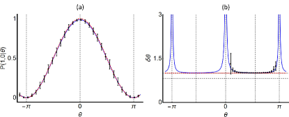
Note that the exact result of $P(+|\theta)$ and the choice of random numbers using Eq. (10) are unneccessary as long as the counts rate has been recorded in real experiment. Furthermore, the phase sensitivity diverges at certain values of $\theta$. Formally, this is because the slope of signal $\partial P(+|\theta)/\partial\theta=0$, but the variance of signal $(\Delta\mu)^{2}\propto P(+|\theta)[1-P(+|\theta)]\neq 0$. Here, the outcome “$+$” represents $n_{1}=1$ and $n_{2}=0$ for the input state $|1,0\rangle$; While for the twin-Fock states $|n,n\rangle$, it stands for the detection event $n_{1}=n_{2}=n$. Due to the experimental imperfections, the signal $P_{\mathrm{fit}}(+|\theta)\neq 0,1$ at certain values of phase shift (e.g., $\theta=0$, $\pm\theta_{\mathrm{dark}}$), so the variance of signal is nonvanishing at that points but the slope of signal is still vanishing, which leads to the singularity of the sensitivity.

References

- (1) G. Brida, M. Genovese, and I. R. Berchera, Nat. Photonics 4, 227 (2010).
- (2) M. A. Taylor, J. Janousek, V. Daria, J. Knittel, B. Hage, H.-A. Bachor, and W. P. Bowen, Nat. Photonics 7, 229 (2013).
- (3) G. B. Lemos, V. Borish, G. D. Cole, S. Ramelow, R. Lapkiewicz, and A. Zeilinger, Nature (London) 512, 409 (2014).
- (4) T. Ono, R. Okamoto, and S. Takeuchi, Nat. Commun. 4, 3426 (2013).
- (5) Y. Israel, S. Rosen, and Y. Silberberg, Phys. Rev. Lett. 112, 103604 (2014).
- (6) M. J. Holland and K. Burnett, Phys. Rev. Lett. 71, 1355 (1993).
- (7) F. W. Sun, B. H. Liu, Y. X. Gong, Y. F. Huang, Z.Y. Ou, and G. C. Guo, Europhys. Lett. 82, 24001 (2008).
- (8) G. Y. Xiang, B. L. Higgins, D. W. Berry, H. M. Wiseman, and G. J. Pryde, Nat. Photonics 5, 43 (2011).
- (9) G. Y. Xiang, H. F. Hofmann, and G. J. Pryde, Sci. Rep. 3, 2684 (2013).
- (10) I. Afek, O. Ambar, and Y. Silberberg, Science 328, 879 (2010).
- (11) J. J. Bollinger, W. M. Itano, D. J. Wineland, and D. J. Heinzen, Phys. Rev. A 54, R4649 (1996).
- (12) J. P. Dowling, Contemp. Phys. 49, 2 (2008); Y. Gao, C. F. Wildfeuer, P. M. Anisimov, H. Lee, and J. P. Dowling, J. Opt. Soc. Am. B 27, A170 (2010).
- (13) C. C. Gerry and J. Mimih, Contemp. Phys. 51, 497 (2010).
- (14) L. Cohen, D. Istrati, L. Dovrat, and H. S. Eisenberg, Opt. Express 22,11945 (2014).
- (15) D. Brivio, S. Cialdi, S. Vezzoli, B. T. Gebrehiwot, M. G. Genoni, S. Olivares, and M. G. A. Paris, Phys. Rev. A 81, 012305 (2010).
- (16) E. Distante, M. Ježek, and U. L. Andersen, Phys. Rev. Lett. 111, 033603 (2013).
- (17) X. M. Feng, G. R. Jin, and W. Yang, Phys. Rev. A 90, 013807 (2014).
- (18) B. Yurke, S. L. McCall, and J. R. Klauder, Phys. Rev. A 33, 4033 (1986).
- (19) B. C. Sanders and G. J. Milburn, Phys. Rev. Lett. 75, 2944 (1995).
- (20) T. Kim, O. Pfister, M. J. Holland, J. Noh, and J. L. Hall, Phys. Rev. A 57, 4004 (1998).
- (21) L. Pezzé, A. Smerzi, G. Khoury, J. F. Hodelin, and D. Bouwmeester, Phys. Rev. Lett. 99, 223602 (2007); L. Pezzé and A. Smerzi, ibid. 100, 073601 (2008).
- (22) L. Pezzé and A. Smerzi, Europhys. Lett. 78, 30004 (2007).
- (23) B. L. Higgins, D. W. Berry, S. D. Bartlett, H. M. Wiseman, and G. J. Pryde, Nature (London) 450, 393 (2007).
- (24) D. W. Berry, B. L. Higgins, S. D. Bartlett, M. W. Mitchell, G. J. Pryde, and H. M. Wiseman, Phys. Rev. A 80, 052114 (2009).
- (25) C. W. Helstrom, Quantum Detection and Estimation Theory (Academic, New York, 1976).
- (26) S. L. Braunstein and C. M. Caves, Phys. Rev. Lett. 72, 3439 (1994); S. L. Braunstein, C. M. Caves, and G. J. Milburn, Ann. Phys. (N.Y.) 247, 135 (1996).
- (27) V. Giovannetti, S. Lloyd, and L. Maccone, Nat. Photonics 5, 222 (2011).
- (28) M. Kitagawa and M. Ueda, Phys. Rev. A 47, 5138 (1993).
- (29) D. J. Wineland, J. J. Bollinger, W. M. Itano, and D. J. Heinzen, Phys. Rev. A 50, 67 (1994); D. Leibfried et al., Science 304, 1476 (2004).
- (30) J. Ma, X. Wang, C. P. Sun, and F. Nori, Phys. Rep. 509, 89 (2011).
- (31) L. Pezzé and A. Smerzi, Phys. Rev. Lett. 102, 100401 (2009); G. Tóth, Phys. Rev. A 85, 022322 (2012).
- (32) B. Lücke, M. Scherer, J. Kruse, L. Pezzé, F. Deuretzbacher, P. Hyllus, O. Topic, J. Peise, W. Ertmer, J. Arlt, L. Santos, A. Smerzi, and C. Klempt, Science 334, 773 (2011).
- (33) R. A. Fisher, Theory of statistical estimation, Proc. Cambridge Philos. Soc. 22, 700 (1925).
- (34) Using the method of Ref.[5], the sensing range of a quantum-enhanced microscopy is about , limited by the optimal work point for phase sensing and the location of dark fringe nearby, .
- (35) D. W. Berry and H. M. Wiseman, Phys. Rev. Lett. 85, 5098 (2000); D. W. Berry, H. M. Wiseman, and J. K. Breslin, Phys. Rev. A 63, 053804 (2001).
- (36) A. Hentschel and B. C. Sanders, Phys. Rev. Lett. 104, 063603 (2010).