Stimulated Brillouin scattering in metamaterials
Abstract
We compute the SBS gain for a metamaterial comprising a cubic lattice of dielectric spheres suspended in a background dielectric material. Theoretical methods are presented to calculate the optical, acoustic, and opto-acoustic parameters that describe the SBS properties of the material at long wavelengths. Using the electromagnetic and strain energy densities we accurately characterise the optical and acoustic properties of the metamaterial. From a combination of energy density methods and perturbation theory, we recover the appropriate terms of the photoelastic tensor for the metamaterial. We demonstrate that electrostriction is not necessarily the dominant mechanism in the enhancement and suppression of the SBS gain coefficient in a metamaterial, and that other parameters, such as the Brillouin linewidth, can dominate instead. Examples are presented that exhibit an order of magnitude enhancement in the SBS gain as well as perfect suppression.
I Introduction
Stimulated Brillouin Scattering (SBS) is a nonlinear opto-acoustic process by which an incident optical pump field generates an acoustic wave inside a dielectric material. The longitudinal acoustic wave compresses the medium periodically to form a diffraction grating, which scatters the incident field; due to the acoustic wave propagation, the scattered field is Doppler shifted to lower frequencies. This amplifies the beating between the Stokes field and the pump field, creating a self-reinforcing effect. Although SBS was theoretically predicted by Brillouin in 1922 Brillouin (1922), it was only after the advent of the laser in 1960 Maiman (1960) that it could be practically realised, with the first experimental paper in SBS following soon after in 1964 Chiao et al. (1964). More recently, research focus has been directed towards the design of practical, small-scale devices that exploit SBS, such as notch-filters, Brillouin lasers, and microwave sources Pant et al. (2014); Morrison et al. (2014); Kabakova et al. (2013); Eggleton et al. (2013). For such device applications, there is considerable interest in materials which exhibit strong SBS, as this allows improved power scaling and subsequently, smaller devices. At the same time, SBS is also regarded as a nuisance in the optical fibre community Peral and Yariv (1999) where SBS acts as a power limit for narrow linewidth signals sent through fibres, and hinders the observation of other nonlinear effects such as four-wave mixing Powers (2011) at power levels above the SBS threshold. Although there are established experimental procedures for overcoming SBS, such as frequency dithering Agrawal (1995), there is considerable interest in designer materials which exhibit intrinsically high, or in certain circumstances, intrinsically low SBS gain.
Here we examine the effects of subwavelength structuring on the intrinsic (bulk) SBS gain spectrum of a material. This work provides an in-depth analysis following our initial observations Smith et al. (2016) in which it was shown that considerable enhancement or complete suppression of the SBS gain can be achieved in a simple cubic lattice of spheres in a background material. In order to characterise the SBS properties of a metamaterial it is necessary to determine a combination of optical, acoustic, and opto-acoustic parameters that feature in the SBS gain spectrum expression Powers (2011); here we give a rigorous formalism whereby these parameters can be computed. To obtain the optical properties (the effective refractive index) we use a long-wavelength homogenisation procedure based on the optical energy density Bergman (1978). For independent validation, we also outline an equivalent procedure which uses the slope of the lowest band surface near the centre of the first Brillouin zone Movchan et al. (2002). To obtain the acoustic properties of the metamaterial we present a long-wavelength procedure, this time using the acoustic energy density, to determine the stiffness tensor and subsequently the longitudinal acoustic velocity for the metamaterial. The remaining acoustic parameters including the frequency shift and line width are obtained by incorporating acoustic damping as a perturbation to the acoustic wave equation. In this way we incorporate the effects of acoustic loss, which is critical to the SBS process, to leading order. The procedure for the opto-acoustic parameter (an element of the fourth-rank photoelastic tensor Newnham (2004)), whilst conceptually simple, is the most technically difficult to obtain and relies on a combination of optical homogenisation and acoustic boundary perturbations.
The solution procedure used makes very few assumptions on the mechanical and optical response of the material, assuming primarly that the constituents are linear elastic dielectric materials in a three-dimensional Bravais lattice configuration. We demonstrate the method for metamaterials comprising a three-dimensional cubic lattice of dielectric spheres embedded in a dielectric background, including simple cubic (sc) and face-centred cubic (fcc) configurations, with a single element per unit cell. These metamaterial designs are chosen not only due to their geometrical elegance, but because they possess closed form expressions in the dilute asymptotic limit, which can be used for numerical validation with suitable approximations. The theoretical framework outlined in the present work is relatively general and can be used to calculate the SBS properties of a wide class of metamaterials.
The outline of this paper is as follows: in Section II we present a brief overview of SBS in isotropic materials, outlining the key material and wave parameters necessary to determine the SBS gain. The following sections then consider techniques to determine these parameters for a metamaterial: In Section III we outline methods to determine the permittivity tensor, in Section IV we present techniques to determine the purely acoustic terms, and in Section V we investigate the photoelastic properties. This is followed in Section VI by a selection of numerical examples and a discussion in Section VII. Appendix A discusses the formal definition of the effective permittivity tensor and Appendix B is an extended comment on the numerical implementation for Section V.
II SBS in isotropic materials
We consider the theoretical framework for an electrostriction-driven backward SBS process in an optically and acoustically isotropic bulk material that exhibits negligible optical losses. Acoustic losses are assumed to be well-modelled through the inclusion of dynamic viscosity effects in the model (linear friction in continuum mechanics), and this is taken to be the dominant loss mechanism for acoustic problems Auld (1973). We also neglect a magnetic response in the metamaterial and additional nonlinear optical effects, such as four-wave mixing. In this setting, we define the total electric field as with
| (1) |
where are the amplitudes, the wave numbers, the angular frequencies of the incident pump field and scattered (Stokes) field, respectively, and is the speed of light in vacuum. The system that describes the intensities of the incident pump and Stokes field takes the form Agrawal (1995); Peral and Yariv (1999); Kobyakov et al. (2010)
| (2a) | ||||
| (2b) | ||||
where , is the vacuum permittivity, and is the refractive index. The SBS power gain spectrum is given by Kobyakov et al. (2010); Powers (2011)
| (3) |
where is the relevant component of the elasto-optic (photoelastic, or, Pockels) tensor for SBS in bulk media, denotes the Brillouin line width with respect to angular frequency, is the wavelength for frequency in vacuum, is the mass density, is the acoustic wave velocity, and is the acoustic wave frequency.
At the Brillouin resonance, a backwards travelling longitudinal acoustic wave is excited with angular frequency , phase velocity and acoustic wave vector . From conservation of momentum, and noting that , we have that
| (4a) | |||
| and subsequently from the dispersion relations for the optical and acoustic problems it follows that | |||
| (4b) | |||
To summarise, knowledge of the material density , the refractive index , the acoustic parameters , and , and the photoelastic tensor element , allows us to determine the bulk SBS power gain at a specified optical wavelength . For reference, a table of bulk material parameters for a range of common materials can be found in Smith et al. (2016). To the best of the authors knowledge, there is no general theoretical treatment of bulk SBS in anisotropic media, however Wolff et al. (2014) has examined SBS in cubic media.
III Optical properties
There are an extensive number of procedures which may be used to determine the optical properties of a composite material at long wavelengths Milton (2002). We outline two methods for determining the effective refractive index; the first having the advantage of being conceptually simple and numerically efficient, but is an indirect method and is only valid for dielectric metamaterials possessing cubic symmetry, and the second being a much more general tool which homogenises the material as opposed to describing wave propagation.
The first and most commonly used approach, is to consider the optical wave equation
| (5a) | |||
| with Bloch–Floquet boundary conditions on the edges of the fundamental cell | |||
| (5b) | |||
| and where the tangential components of and are continuous across all dielectric interfaces : | |||
| (5c) | |||
Here is the matrix representation of the relative permittivity tensor , denotes the magnetic field of the Bloch mode, is the normal vector to the boundary of the th inclusion, denotes the jump discontinuity in the field across the interface, is defined with respect to a conventional Cartesian basis, is the real lattice vector, and denotes the edges of the entire fundamental cell. For a cubic lattice for , and is the period.
The optical boundary value problem described by (5a)-(5c) is then numerically solved for a Bloch vector sufficiently close to the point, i.e. . Using the lowest angular eigenfrequency the effective refractive index is obtained via
| (6) |
This procedure only applies to cubic metamaterials, and is an indirect method for characterising the optical properties of the medium. This is because the refractive index describes wave propagation whereas the permittivity is an intrinsic material property. Such a shortcoming can easily be overcome by considering an alternative procedure; a modification of the method outlined in Bergman (1978) which we term an energy density method. We introduce this procedure by considering the approach for a metamaterial of cubic symmetry. As before, it requires that we solve (5a)-(5c) for a wave vector close to , except we now compute the volume-averaged electromagnetic energy density
| (7a) | |||
| where is the volume of the Wigner-Seitz cell Kittel (2005). This quantity is then equated to an effective energy density ansatz | |||
| (7b) | |||
| to obtain the scalar effective permittivity | |||
| (7c) | |||
Since our cubic metamaterial comprises dielectric media and is examined in the long wavelength limit, we take throughout and so follows immediately. We remark that there is no difference in the numerical result obtained using either (6) or (7c) . The equivalence of the two effective medium methods outlined in this section can be found in Appendix A, where it is shown that the equivalence holds provided is parallel to a principal axis vector. The primary motivation for using (7c) can be found in later sections, when we require the effective permittivity tensor for the metamaterial under an applied strain. When the metamaterial is strained the symmetry class changes, and subsequently a generalisation of (7c) is required. By evaluating the permittivity tensor directly, we avoid the added step of reverse engineering the effective permittivity tensor from multiple scalar refractive index values.
The generalisation of (7c) for other lattice configurations takes the form
| (8) |
where denotes principal dielectric constants Born and Wolf (1999). These constants are defined with respect to the principal dielectric axes of the metamaterial. In order to obtain an invertible linear system for the three unknown , we consider three different Bloch vectors near the point that are parallel to the principal dielectric axes of the metamaterial. Once the principal permittivities are obtained, the effective permittivity tensor is obtained via a change of basis operation, as the effective permittivity is defined with respect to the Cartesian coordinate axes. For cubic and tetragonal metamaterials, for example, it can be shown that . Note that the principal dielectric axes of monoclinic and triclinic metamaterials cannot be predicted a priori and in such instances this procedure cannot be used.
IV mechanical properties
Next we consider the mechanical parameters of our metamaterial, and proceed with the simplest of these; determining the material density, which is given by simple volume averaging. Explicitly, given the filling fraction of the inclusion material in the background material, the density is given by
| (9) |
where denote the mass densities of the inclusion and background material, respectively.
We now compute the acoustic phase velocity at long wavelengths, where in the absence of acoustic loss, the governing equation is Auld (1973)
| (10a) | |||
| where denotes the mechanical displacement from equilibrium, is the fourth-rank stiffness tensor, is the strain tensor, (defined as the symmetric gradient of the displacement: ), the symbol denotes the inner product between a fourth- and second-rank tensor, and we consider time harmonic solutions of the form . (10a) is solved with the Bloch condition | |||
| (10b) | |||
| which is defined with respect to the acoustic Bloch vector , and assuming continuity of the mechanical displacement field and vanishing normal stress across all mechanical interfaces | |||
| (10c) | |||
where denotes the stress tensor. It is from the boundary-value problem described in (10a)–(10c) above that we determine the phase velocity for the longitudinal acoustic wave excited by SBS in a metamaterial. A conventional approach, which is valid when the material is structured to form a cubic crystal, is to simply consider an acoustic wave vector at the SBS resonance and use the angular frequency corresponding to the approximately longitudinal mode, to obtain
| (11) |
This method (which implicitly assumes that is also sufficiently close to the point) is only applicable to highly symmetric problems, and accordingly, a more general approach is required.
The procedure we consider here is analogous to that used for determining the effective permittivity in Section III, except we now consider the elastodynamic energy density to determine the effective fourth-rank stiffness tensor for the metamaterial. For a given acoustic Bloch vector we compute the volume-averaged strain energy density
| (12a) | |||
| and equate this to an effective strain energy density ansatz | |||
| (12b) | |||
| to obtain the system | |||
| (12c) | |||
Assuming symmetric stress and strain tensors, reversible deformations, and a metamaterial with cubic symmetry, the total number of unknown coefficients is reduced from 81 to 3 (these are , , and ) making the calculation in (12c) above tractable.
Having determined the coefficients, expressions for the acoustic phase velocities (quasi-longitudinal , quasi-shear and pure shear ) follow from the acoustic dispersion equation of an isotropic, cubic material. For any cubic material with an acoustic wave vector oriented along a crystal axis we have Auld (1973)
| (13) |
where the longitudinal wave speed is the velocity term present in the SBS gain coefficient.
We now evaluate the two remaining mechanical parameters necessary to evaluate the SBS gain coefficient in (3) for a metamaterial: the Brillouin frequency shift and Brillouin line width . These parameters are obtained by incorporating the effects of mechanical loss into (10a) above. In general terms, the inclusion of loss alters the eigenvalues of the acoustic wave equation to make them complex-valued, with the frequency shift and line width given by the real and imaginary components of the appropriate eigenvalue (see (15) below). For an SBS process, the acoustic mode is purely longitudinal and so we consider the acoustic frequency which lies on the first longitudinal band surface at the resonant acoustic wave vector . We begin by assuming that mechanical losses can be modelled, at least to leading order, by including phonon viscosity effects in our model. Subsequently, is replaced by in the acoustic wave equation (10a) where denotes the fourth-rank dynamic phonon viscosity tensor. Provided for all indices, we treat the effect of phonon viscosity as a perturbation to the acoustic frequencies of the lossless mechanical problem. If we take the dot product of (10a) with and integrate over the unit cell, the eigenvalues take the form where
| (14) |
The Brillouin frequency shift and the acoustic damping are obtained from the longitudinal acoustic frequency by simply evaluating a square root to obtain
| (15) |
Note that we have used the convention of examining complex frequency and real Bloch vector, which follows from our representation of the SBS gain coefficient in (3) (for a formalism in terms of the incident wave vector, see Wolff et al. (2015)).
V Photoelastic properties
In this section we determine the photoelastic tensor element present in the gain spectrum expression (3). The photoelastic tensor of a material is implicitly defined via
| (16) |
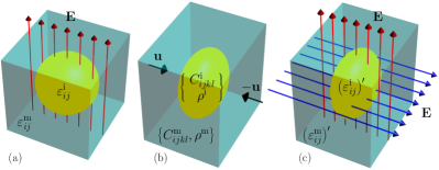
where denotes the change in the inverse relative permittivity tensor and denotes the fourth-rank photoelastic tensor. The procedure we use to determine for a cubic metamaterial is presented schematically in Figure 1 and we outline this in detail.
First, we compute the effective inverse permittivity tensor for the unstrained unit cell (Figure 1(a)).
Second, we compress the unit cell by imposing displacements on the cell boundary to obtain the strained unit cell and the internal strain field (Figure 1(b)). We solve the acoustic wave equation (10a) in the static limit with the boundary conditions
| (17) |
where denote the faces of the cubic cell with normal vectors and is the positive-valued amplitude of the imposed displacement. These boundary conditions give a strain across the unit cell of . Under this compression, the inclusion geometries inside the cell are deformed and the constituent permittivity tensors are now anisotropic following (16). For example, in the background material we have
| (18) |
Third, we return to the procedure outlined in Section III and compute the effective permittivity for the strained cell with strained constituent permittivities (Figure 1(c)). A cubic crystal under an strain possesses tetragonal symmetry, and so the strained permittivity tensor is uniaxial. Subsequently, two subwavelength Bloch vectors are necessary to calculate the effective tensor (8). Comparing the change in inverse permittivity tensors for the imposed strain gives
| (19) |
We remark that for cubic crystals there are only three free parameters in the full photoelastic tensor, and the structure of the tensor means that only one simple strain need be considered to recover the effective photoelastic term for the SBS gain (3).
In the event that all 36 elements of the photoelastic tensor are required, further imposed displacement fields must be considered. For example, the component can be obtained by applying an strain which corresponds to the boundary conditions
however care must be taken to correctly determine the principal axes of the sheared cell.
VI Numerical results
To illustrate the procedure outlined in previous sections, we consider simple cubic (sc) and face-centred cubic (fcc) lattices of spheres in a background material, with one sphere per lattice site. We emphasise that these configurations are chosen as they admit closed-form expressions in the dilute limit, which is useful for independent validation Smith et al. (2015). However, our method applies generally to all periodic structures for which an effective and can be obtained. Due to complexities in numerical implementation (see Appendix B) we restrict our attention to filling fractions below the dense packing limit; explicitly, we consider the range for sc lattices and for fcc lattices. The dense packing limit is for an sc lattice and for an fcc lattice, below which the filling fractions are given explicitly by
| (20) |
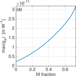
where denotes the radius of the spherical inclusions and the period of the cubic lattice. Above the dense packing limit, the filling fraction can be easily evaluated numerically. In the figures that follow, the SBS gain coefficient is obtained by specifying in (3) to give
| (21) |
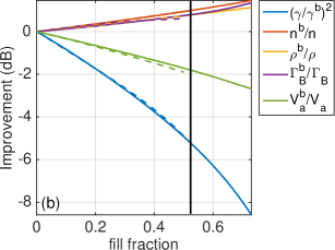
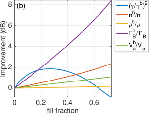
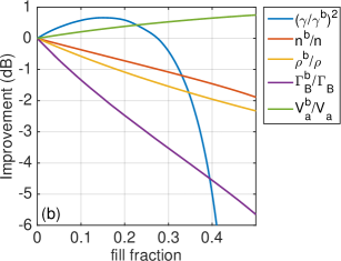
where denotes the electrostrictive stress. We also examine the contribution from each term in (21) as the filling fraction is changed by considering:
| (22) |
where the superscript denotes the bulk parameter value for the background material. In this way, the contribution from each term to the enhancement, or suppression, of the SBS gain coefficient can be straightforwardly determined by simply adding the value given by each curve at a specified filling fraction.
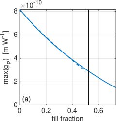
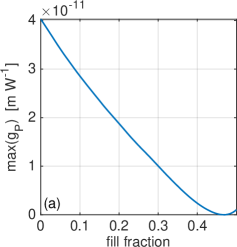
In Figure 2a, we show the gain coefficient as a function of filling fraction, for an sc and fcc lattice of SiO2 spheres in an otherwise uniform As2S3 background. In this figure, we observe that the suppression of the gain coefficient is almost entirely independent of the lattice configuration for . This suggests that the result is independent of any lattice configuration (including random), since the metamaterial structuring is both optically and acoustically subwavelength. At we achieve a suppression of the background gain coefficient and at (fcc) we achieve a suppression of 82%. As a result, the power threshold for SBS in As2S3 has been raised considerably. Note that when calculating these percentages we have used at , which is within 10% of experimentally obtained values for the gain coefficient in As2S3 waveguides Pant et al. (2011). A solid black vertical line is shown at which marks the dense packing threshold for sc lattices of spheres.
In Figure 2b we determine the contribution from each term present in (21), as seen in (22), and observe that reduced electrostriction is the primary mechanism behind the suppressed gain coefficient, followed by the increased longitudinal acoustic velocity. All other terms work to enhance the gain coefficient, however the electrostriction and acoustic velocity terms outstrip these contributions to suppress the gain coefficient overall. The solid curves denote results for the fcc lattice and broken lines denote an sc lattice, where as in Figure 2a, the difference is negligible between the two lattice types over .
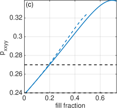
Although Figure 2b demonstrates suppression in the electrostriction parameter for SiO2 spheres in As2S3, the photoelastic constant is actually increasing, as can be seen in Figure 2c. Here, we superimpose the result for sc (dashed blue curve) and fcc (solid blue curve) lattices, where dashed horizontal black lines denote the intrinsic for the constituent materials. It is immediately apparent that the photoelastic constant for the metamaterial is not given by a simple mixing of the two constituent values, but instead, also includes a strong artificial photoelasticity contribution Smith et al. (2015) that arises due to the different mechanical responses of the constituent media. As in the preceding figures, the difference between the sc and fcc lattice configurations is minor, and the value of at is extremely close to the maximum value obtained for at . The explanation for the suppressed electrostriction parameter lies in the reduced effective index of the two materials; although the effective photoelastic term is increasing strongly, the effective permittivity is decreasing at a faster rate, and so suppressed electrostriction results overall.
In Figure 3a, we show the maximum gain coefficient for an fcc lattice of SiO2 spheres in Si, which shows a monotonically increasing SBS gain coefficient from at to at , and corresponds to more than one order of magnitude enhancement (an enhancement of 13.3 compared to the background value). Referring to Figure 3b, it is immediately apparent that electrostriction is not the primary mechanism for the enhancement in the gain coefficient, it is instead the Brillouin linewidth. Given that our earlier work Smith et al. (2016) suggests electrostriction is the force majeure behind the enhancement and suppression of the gain coefficient, this is an important demonstration that all terms in (21) must be calculated in order to determine the SBS properties of a composite material, and that it is incorrect in general to rely on the electrostriction alone. In this example, the electrostriction achieves a maximum of at , returning to the electrostriction value for the background material at . Over the range all terms contribute positively to enhance the gain coefficient, after which the electrostriction acts to suppress the gain coefficient.
The final example we consider is an sc lattice of GaAs spheres in SiO2 as shown in Figure 4. Here, the gain coefficient is completely suppressed at a filling fraction of and can be attributed to a perfectly vanishing photoelastic parameter. In this example, the increased linewidth acts as the primary mechanism behind the suppression of SBS from , after which the vanishing electrostriction term dominates. From Figure 4b, we observe that the electrostriction reaches a maximum of at before returning to the background material value at and ultimately reaching a zero near . The only parameter that consistently works against the suppression of the SBS gain is the acoustic velocity. Note that at we have which differs by from experimental data for the gain coefficient in fused silica waveguides Abedin (2005).
VII Discussion
We have presented a rigorous procedure for determining all material and wave propagation parameters that feature in the SBS gain coefficient for a metamaterial. This involves intensive numerical calculations for the optical properties, mechanical properties, and photoelastic properties present in (3). The implementation of routines to evaluate these parameters is complicated, as discussed in Appendix B, but have been successfully used to demonstrate both enhancement and suppression of the SBS gain coefficient in composite media. We have demonstrated that for arrays of spheres, the SBS gain is independent of the cubic lattice configuration, provided the metamaterial is optically and acoustically subwavelength. Also, we have shown that electrostriction does not always completely determine the behaviour of the SBS gain coefficient; the Brillouin linewidth is shown to play an important role for certain material combinations.
The methods will enable researchers to characterise the SBS properties of exotic metamaterials, which may open promising new paths for opto-acoustics and SBS. Materials with enhanced or suppressed gain coefficients are of particular interest for on-chip applications.
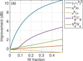
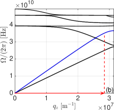
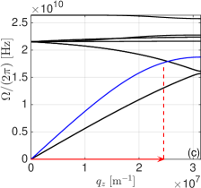
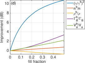
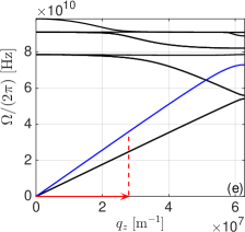
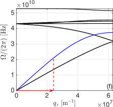
We note that the quasi-static assumptions necessary for a number of steps in our procedure require that we have a sufficiently large number of unit cells per optical and acoustic wavelength in the material. It is only in this setting that the descriptions presented in this paper are valid. To demonstrate this point we include Figure 5 where results for an sc lattice of As2S3 spheres in Si for and can be found. In Figure 5a we observe that the acoustic parameter decreases at first, to reach a local minimum at , before increasing in a predictable manner. The explanation for this behaviour can be found in Figures 5b and 5c where we compute the acoustic band structure at and filling fractions. The high effective refractive index for these structures means that the magnitude of the SBS resonant wave vector is large. Consequently, the acoustic wave vector is no longer sufficiently close to the point and so results are incorrect. Reducing the lattice period to for example, scales the band structure of the material such that the acoustic wave vector is then within a neighbourhood of where effective acoustic parameters can be computed (Figures 5d–5f). Note that if the period of the lattice is sufficiently large, then and we exit the first Brillouin zone, potentially giving rise to acoustic Umklapp scattering.
We also remark that considerable care must be taken to ensure the symmetry properties of effective material tensors are correctly characterised: the symmetry of the underlying lattice (i.e., cubic), the symmetry of the inclusion geometry, or structure inside the cell, and the symmetry of the constituent tensors (i.e., the permittivity or stiffness tensor), are all relevant in determining the symmetry of the effective tensor.
Although not directly required for evaluating the SBS gain coefficient, the viscosity tensor for a metamaterial can also be evaluated using energy density methods. In order to determine this tensor we use the dissipative power, which represents the rate of energy loss in the material, in place of the acoustic energy density (12a). The dissipative power is given by , or , which amounts to a careful scaling of the approach used to determine .
Acknowledgements
This work was supported by the Australian Research Council (CUDOS Centre of Excellence, CE110001018).
Appendix A Definition of the permittivity tensor
In this section we discuss the relationship between the methods outlined here for characterising the optical properties of the structured material; the energy density method for the effective permittivity, and using the slope of the first band surface near the point to retrieve the effective refractive index.
We begin by considering the electromagnetic energy density differential Landau et al. (1984)
| (23) |
from which the electric displacement is given by
| (24) |
which assumes no perturbation to the field (no change to the magnetic susceptibility). Using the definition of the energy density where is the Poynting vector and the group velocity Auld (1973), it follows from (24) that
| (25) |
where denotes a Cartesian basis vector. Next we assume that the material exhibits a linear optical response
| (26) |
where for simplicity, we consider an isotropic and homogeneous material which admits
| (27) |
where is the phase velocity. Thus, the permittivity of an isotropic material is given by the inverse product of the group and phase velocities of the medium. In the long wavelength limit and so it follows that . For an anisotropic and homogeneous material the energy density method works when the unit vector is oriented along one of the principal axes of the permittivity tensor. Along other directions this treatment fails, which is obvious considering the complex geometries of the isofrequency contours for optically biaxial media, for example.
Appendix B Numerical implementation of the effective photoelasticity method
All results presented in the present work were obtained using COMSOL . We emphasise that COMSOL was not developed with this application in mind, and so we outline the procedure to obtain for a cubic metamaterial, following the schematic in Figure 1.
Step (a): the procedure for calculating the effective permittivity of an unstrained unit cell is straightforward. Implementing an ‘Eigenfrequency Study’ inside the ‘RF module’ for gives a desired set of eigenfrequencies, and we compute (7c) using the electric field mode corresponding to the smallest genuine eigenvalue (note the TE and TM modes are degenerate along in the vicinity of the point). There are two issues when using the standard solver; the first is that an estimate for the lowest eigenfrequency must be specified. Even after specifying this shift, the lowest eigenvalues are often spurious modes that must be discarded. The second issue is that the Bloch vector cannot be arbitrarily small; we recommend specifying where is a small parameter, and scaling the small parameter until is sufficiently close to the point (for example, ). As mentioned in Section III, the optical wave equation (5a) for the full cell imposes Bloch conditions on all boundaries of the unit cell , however the convergence of eigenfrequencies using the full cell is slow and requires considerable computational power. Convergence can be significantly accelerated by using a reduced unit cell geometry.
Specifically, if we consider metamaterials with cubic symmetry and principal axes parallel to a Cartesian basis vector (i.e., ) then we can exploit the symmetry of the problem in order to reduce our computational domain and thereby accelerate convergence. In other words, we halve the geometry of the unit cell in each of the remaining Cartesian basis vector directions (i.e., and ), leaving of the original cell. Depending on whether the TE or TM polarised solutions are sought, we impose PEC conditions on the edges of the reduced cell in one direction (i.e., on where denotes the boundary of the reduced cell) and PMC conditions in the remaining direction (i.e., on ), with Bloch conditions imposed on . Since we are sufficiently close to the point (i.e., ), the modes for both TE and TM polarisations are degenerate at long wavelengths. Accordingly, provided one reduced boundary has PMC conditions and the other has PEC, then the correct effective permittivity is obtained.
Step (b): The strained reduced unit cell and corresponding internal strain field are obtained through a Stationary Study of a linear elastic material in the Solid Mechanics module of COMSOL 4.4. We emphasize strongly that the calculation outlined here is one of a strain and not of a stress on a three-dimensional unit cell. Since the problem is symmetric for the simple strain we consider, the unit cell geometry can also be reduced, which formally restrict solutions to one symmetry class (i.e., longitudinal solutions). For the reduced unit cell, the boundary conditions in the reduced directions (i.e., on and ) are vanishing normal displacement . To induce an strain, we impose the displacements (17) on . From the longitudinal mode a strain tensor can be computed inside the unit cell. This strain field is exported as several text files for each domain, along with the domain number. We then import these data files into MATLAB so that the strained permittivity tensor inside each deformed domain can be calculated as in (18). The meshing for this problem must exploit all possible symmetries to ensure numerical stability in Step (c). Note that an artificial boundary must be introduced at and the mesh for all boundaries with must be identical.
Individual text files corresponding to each domain are generated in MATLAB, which contain the strained permittivity tensor as a function of discretized coordinates inside each domain. This is done to ensure the permittivity tensor is uniquely and correctly assigned in Step (c) without encountering interpolation issues across domain boundaries. We remark that the strained unit cell geometry can only be exported when ‘Geometric Nonlinearity’ is included in the model. With this functionality enabled, the strained unit cell is exported as a deformed mesh file using the ‘Remesh deformed configuration’ option (as an mphtxt file). The geometric nonlinearity will calculate different stress and strain tensors and so care must be taken to use the Engineering strain tensor for our analysis, as this corresponds to the linear theory treatment presented here. In practice, there is little difference between the linear and nonlinear strain tensors for unit cells that are strongly subwavelength and subject to small strains.
Step (c): This repeats the processes outlined in Step (a), except that we import the geometry (the mphtxt file) and define all six elements of the permittivity tensor in each domain using interpolated functions. Even if the strained unit cell is computed with an extremely dense mesh, it is still often necessary to ‘repair’ the geometry, until COMSOL recognises the correct number of boundaries and domains. This is a nontrivial step and the ‘repair tolerance’ must be carefully chosen. Once all six permittivity tensor elements are imported and defined inside each and every domain as interpolated functions, these must then be assigned to a ‘Material’ for each domain. Solving the optical wave equation (5a) for the reduced and strained cell configuration, we obtain the first linear equation of the two equations necessary to determine the effective permittivity tensor (see (8)). To obtain the second linear equation using a reduced cell geometry, it is necessary to solve the optical wave equation problem for . Accordingly, we use the Geometry tools in COMSOL to delete half of the existing cell geometry, copy the remaining geometry, and then reflect the copied geometry about to obtain the appropriate reduced cell. Assigning Materials classes to the reflected domains using where appropriate, and imposing PMC and PEC conditions on the reduced directions ( and ), we obtain the final eigenvalue problem. Solving this for we evaluate (8) once more to obtain the second linear equation, and subsequently the strained effective tensor.
References
- Brillouin (1922) L. Brillouin, Ann. Phys.(Paris) 17, 21 (1922).
- Maiman (1960) T. Maiman, Nature 187, 493 (1960).
- Chiao et al. (1964) R. Chiao, C. Townes, and B. Stoicheff, Phys. Rev. Lett. 12, 592 (1964).
- Pant et al. (2014) R. Pant, D. Marpaung, I. V. Kabakova, B. Morrison, C. G. Poulton, and B. J. Eggleton, Laser Photonics Rev. 8, 653 (2014).
- Morrison et al. (2014) B. Morrison, D. Marpaung, R. Pant, E. Li, D.-Y. Choi, S. Madden, B. Luther-Davies, and B. J. Eggleton, Opt. Comm. 313, 85 (2014).
- Kabakova et al. (2013) I. V. Kabakova, R. Pant, D.-Y. Choi, S. Debbarma, B. Luther-Davies, S. J. Madden, and B. J. Eggleton, Opt. Lett. 38, 3208 (2013).
- Eggleton et al. (2013) B. J. Eggleton, C. G. Poulton, and R. Pant, Adv. Opt. Photonics 5, 536 (2013).
- Peral and Yariv (1999) E. Peral and A. Yariv, IEEE J. Quantum Elect. 35, 1185 (1999).
- Powers (2011) P. E. Powers, Fundamentals of nonlinear optics (CRC Press, Boca Raton, 2011).
- Agrawal (1995) G. P. Agrawal, Nonlinear fiber optics, 2nd ed. (Academic press, San Diego, 1995).
- Smith et al. (2016) M. J. A. Smith, B. T. Kuhlmey, C. M. de Sterke, C. Wolff, M. Lapine, and C. G. Poulton, Opt. Lett. 41, 2338 (2016).
- Bergman (1978) D. J. Bergman, Phys. Rep. 43, 377 (1978).
- Movchan et al. (2002) A. B. Movchan, N. V. Movchan, and C. G. Poulton, Asymptotic models of fields in dilute and densely packed composites (World Scientific, 2002).
- Newnham (2004) R. E. Newnham, Properties of Materials: Anisotropy, Symmetry, Structure: Anisotropy, Symmetry, Structure (Oxford University Press, New York, 2004).
- Auld (1973) B. A. Auld, Acoustic fields and waves in solids (John Wiley & Sons, 1973).
- Kobyakov et al. (2010) A. Kobyakov, M. Sauer, and D. Chowdhury, Adv. Opt. Photonics 2, 1 (2010).
- Wolff et al. (2014) C. Wolff, R. Soref, C. Poulton, and B. Eggleton, Optics express 22, 30735 (2014).
- Milton (2002) G. W. Milton, The Theory of Composites (Cambridge University Press, Oxford, 2002).
- Kittel (2005) C. Kittel, Introduction to solid state physics (Wiley, 2005).
- Born and Wolf (1999) M. Born and E. Wolf, Principles of optics electromagnetic theory of propagation, 7th ed. (Cambridge University Press, 1999).
- Wolff et al. (2015) C. Wolff, M. J. Steel, B. J. Eggleton, and C. G. Poulton, Phys. Rev. A 92, 013836 (2015).
- Smith et al. (2015) M. J. A. Smith, B. T. Kuhlmey, C. M. de Sterke, C. Wolff, M. Lapine, and C. G. Poulton, Phys. Rev. B 91, 214102 (2015).
- Pant et al. (2011) R. Pant, C. G. Poulton, D. Y. Choi, H. Mcfarlane, S. Hile, E. Li, L. Thevenaz, B. Luther-Davies, S. J. Madden, and B. J. Eggleton, Opt. Expr. 19, 8285 (2011).
- Abedin (2005) K. S. Abedin, Opt. Expr. 13, 10266 (2005).
- Landau et al. (1984) L. D. Landau, E. Lifshitz, and L. Pitaevskii, Electrodynamics of continuous media, Vol. 8 (Pergamon Press, Oxford, 1984).