Yokohama to Ruby Valley : Around the World in 80 Years. II.

Abstract

We two had year-long research leaves in Japan, working together fulltime with several Japanese plus Tony De Groot back in Livermore and Harald Posch in Vienna. We summarize a few of the high spots from that very productive year ( 1989-1990 ), followed by an additional fifteen years’ work in Livermore, with extensive travel. Next came our retirement in Nevada in 2005, which has turned out to be a long-term working vacation. Carol narrates this part of our history together.

I To Yokohama from Livermore

I first met Bill in 1972 as a student in his graduate courses in Statistical Mechanics and Kinetic Theory. I had the welcome opportunity to work part time at the Lawrence Livermore National Laboratory (LLNL) as a “student employee” while enrolled in the PhD program at the Department of Applied Science (DAS) in the University of California at Davis-Livermore. Although I had selected a talented thesis advisor, John Killeen, who specialized in computational plasma physics, I recall thinking at the time that I would have enjoyed thesis research with Bill. His classes were both stimulating and challenging!

Sixteen years later I was a Group Leader for the National Magnetic Fusion Energy Computer Center (NMFECC) where innovations in computer hardware and software led to the first interactive operating system, to the first unclassified national network, and to the era of the Cray supercomputers. I taught scientists and engineers the implementation and use of algorithms on computers still in the design phase. By then my interests had broadened to include finite-element simulations.

I helped many plasma physicists to vectorize their software. One of them, a Professor Sumnesh Gupta from Lousiana State University, asked me to arrange a meeting with Bill during his visit. Bill is and was decisive. When I went to check on his meeting with Professor Gupta he asked me “How about dinner?” My reply was, “Are you serious ?” ! That was the beginning of our wonderful life-long partnership. We were married less than a year later.

In 1988 we visited Cornell. Bill met with Ben Widom and his chemistry colleagues while I met with a group specializing in transputer-based parallel systems. The Crays were becoming prohibitively expensive and were nearing their speed limits. What we learned at Cornell was sufficiently exciting that on our return to Livermore we contacted another DAS PhD, Tony De Groot. His thesis research analyzed arrays of interconnected low-cost transputers with a fast network, providing a parallel architecture alternative to the vector parallelism used in the Cray supercomputers. Tony had a grant to build a prototype system with 64 processors and to demonstrate its speed for an interesting physics or engineering problem. Figure 1 shows a snapshot from the project. Tony’s work was a perfect match for our interests in a future with parallel computers, molecular dynamics, materials science, and continuum mechanics all linked together.

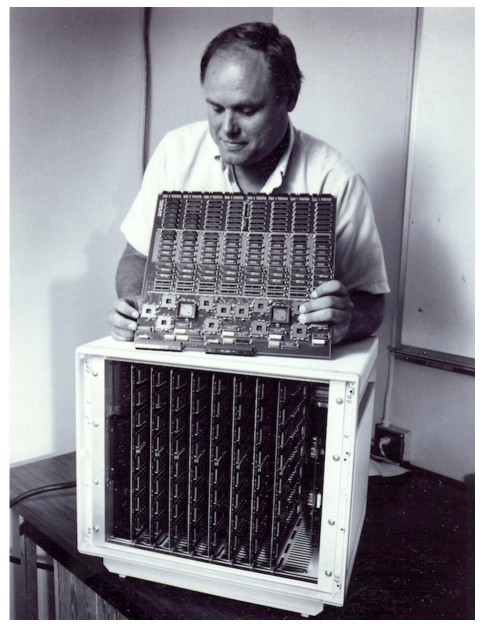
Figure 1: ( Systolic Processor with Reconfigurable Interconnection Network of Transputers ).

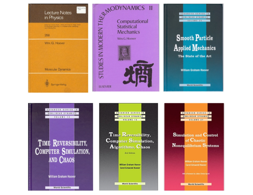
Figure 2: Bill has written six books. He completed the second book, Computational Statistical Mechanics, while we were in Japan. Harald Posch gave Bill the Boltzmann stamp and Shuichi Nosé furnished the kanji on the cover. The two-part kanji “entropy” combines those for “heat” and “divide”.

I.1 Research Leave, Sabbatical, and a Collaboration in Japan, 1989-1990

In 1989 it was time for Bill’s third Sabbatical Leave from DAS. Bill was invited to Japan to visit Shuichi Nosé at Keio University in Yokahama. I was invited to work with Professor Toshio Kawai, who headed up the same physics department. We both had supporting grants, Bill’s from the Japan Society for the Promotion of Science and mine a research and teaching grant from LLNL.

We spent the academic year 1989-1990 in Nosé’s Keio University laboratory. Officially I was working with Professor Kawai, who had an interest in statistical mechanics while Bill was working with Shuichi Nosé. But in reality we both worked together with Professor Taisuke Boku, a parallel-computing specialist, and a physicist Sigeo Ihara at Hitachi’s Kokubunji Laboratory. Our common interest was large-scale molecular dynamics problems involving plastic flow. This work was coordinated with several colleagues back at Livermore as well as Brad Holian at Los Alamos. Tony De Groot made the project possible. He successfully designed and built the SPRINT computer which he could run fulltime, at Cray speed, in his office.

We were also collaborating with Harald Posch in Wien on Lyapunov spectra for many-body chains and pendulab1 while writing a book on Computational Statistical mechanicsb2 . See Figure 2. Bill’s Son Nathan, who had married us back in Livermore, was working at Teradyne Tokyo, and accompanied by his Wife Megumi, throughout our research leaves in nearby Yokohama, leading to many Family get-togethers, often with our Japanese colleagues and their Families.

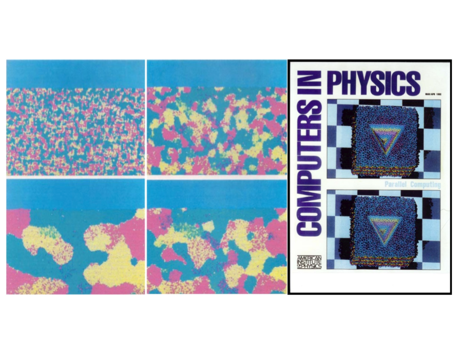
Figure 3: The left panel shows the annealing of an initially unstable square lattice using a combined Lennard-Jones and embedded-atom potential. This sample was used as the initial condition for modelling the indentation of copper. We simulated the indentation of silicon in three dimensions with both atomistic and planar-surface indentors. The speed of the million-atom simulation on the 64-processor SPRINT equalled the speed of a Cray-2. The picture shown on the right appeared on the cover of Computers in Physics in 1992 and illustrates the indentation of 373,248 silicon atoms.

I.2 Large-Scale Molecular Dynamics Simulations – “Plastic Flow”

Our biggest project in Japan involved a Baker’s dozen of physicists, engineers, and computer scientists. The goal was to model, visualize, and analyze million-atom two- and three-dimensional “plastic flows”, flows of solids in response to shear stress. The two-dimensional work allowed us to study the kinetics of grain formation during annealing. See Figure 3. The three-dimensional work modeled the indentation of silicon and ductile metals using angle-dependent and embedded-atom force models in the dynamics. All of this many-body work was carried out on Tony’s SPRINT computer. As fast as a CRAY, SPRINT was put together with $30,000 worth of transputers rather than $30,000,000 of CRAY hardware. This collaboration resulted in several papers over a six-year period, one of them with nine authors, three in Japan, three in Livermore, Brad at Los Alamos, plus Bill and meb3 ; b4 ; b5 . Late at night in the Kawai Lab Bill was writing his Computational Statistical Mechanics book with some help from me.

II Fifteen Years at the Livermore Laboratory, 1990-2005

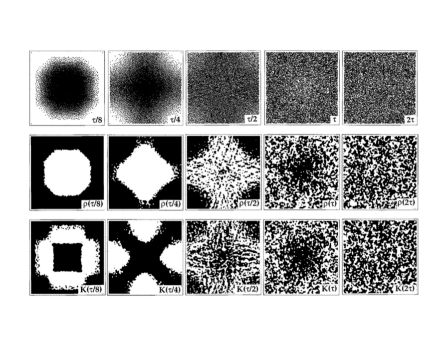
Figure 4: Snapshots of a 16,384 particle simulation of the four-fold adiabatic expansion of an ideal gas, using Lucy’s weight function with $h=6$. The individual particle locations, as well as grid-based contour representations of the density and kinetic energy, are shown at times of $(\tau/8),(\tau/4),(\tau/2),(\tau),(2\tau)$ where $\tau$ is the sound traversal time. The contour plots of the density ( middle row ) and the kinetic energy ( bottom row ) show above-average regions in white and below-average in blackb14 . The density change in expansion is from 1 to 0.25 .

The background of the 1980s was foundational for our research at Livermore : Howard Hanley’s 1982 Boulder Conference “Nonlinear Fluid Behavior”b6 ; Nosé’s two 1984 papersb7 ; b8 ; Bill’s followup “Nosé-Hoover” paperb9 ; and Giovanni Ciccotti and Bill’s 1985 Fermi Schoolb10 “Molecular-Dynamics Simulation of Statistical-Mechanical Systems”. These beginnings soon led to the discovery of the ubiquitous fractal distributions stemming from time-reversible simulations consistent with the Second Law of Thermodynamicsb11 . Bill and I, along with many of those in this room, as well as our hundreds of colleagues, have explored and analyzed thousands of different model systems so as to flesh out the connection of time-reversible microscopic mechanics with irreversible macroscopic thermodynamics and computational fluid dynamics.

The goal for this period was a consistent and comprehensive view of macroscopic and microscopic nonequilibrium systems. These were years of exploration and learning, applying dynamical-systems methods to small and large atomistic simulations. Gibbs’ phase-space description, augmented by feedback and constraints, relates entropy change to the action of thermostats extracting the irreversible heat generated by velocity or temperature gradients. Here we review a few examples. We consider macroscopic nonequilibria first, taking up an algorithm resembling molecular dynamics but developed in order to solve continuum problems, Smooth-Particle Applied Mechanics, SPAM.

II.1 The Structure of Smooth-Particle Applied Mechanics = SPAM

SPAM was developed in 1977 by Lucy and by Monaghan and Gingold at Cambridgeb12 ; b13 . They solved large-scale astrophysical problems by ascribing all of the many continuum properties ( density, velocity, energy, stress, heat flux . . . ) to a mesh-free set of moving particles. This same idea can be applied to traditional problems in computational fluid dynamics such as shockwave structure and Rayleigh-Bénard convection. It can also be merged with molecular dynamics, defining an equivalent continuum within which the moving particles serve as interpolation points. The key idea is the smooth-particle interpolation scheme : localized particle properties are patched together to generate global very smooth doubly-differentiable continuum fields. These fields are constructed by summing particle contributions with a weight function which has two continuous derivatives at the cutoff distance $h$ :

$$w_{\rm Lucy}(r<h)=C_{D}[\ 1+3(r/h)\ ][\ 1-(r/h)\ ]^{3}\ .$$

The range $h$ of the weight function is chosen to include a few dozen particles. For simplicity here we choose to use particles of unit mass. The normalization constant $C_{D}$ depends upon the dimensionality $D$ of the problem :

$$C_{1}=(5/4h)\ ;\ C_{2}=(5/\pi h^{2})\ ;\ C_{3}=(105/16\pi h^{3})\longleftrightarrow\int w{\rm dV}\equiv 1\ .$$

Though ( many ) other weight functions can be used Lucy’s is the simplest polynomial that satisfies the constraints of a smooth maximum with two vanishing derivatives at the maximum distance $h$ .

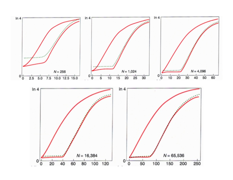
Figure 5: Time development of the “laboratory-frame” entropy ( upper curve ), “comoving” “Lagrangian-frame” entropy ( lower curve ), as well as a fixed-grid-based version of the comoving entropy ( dots ) for systems of 256, 1024, 4096, 16384, and 65536 particles. The time interval shown is one-half the sound traversal time in each case. The entropy range shown is $Nk\ln(4)$ in each case.

Fluid simulations solve ordinary differential equations for the three particle properties $\{\ r_{i},v_{i},e_{i}\ \}$ . From these and the gradients which can be derived from them by differentiation all the continuum properties $\{\ \rho(r),u(r),e(r),\sigma(r),Q(r),...\ \}$ follow :

$$\rho(r)=\sum_{i}w(r-r_{i})\ ;\ \rho(r)u(r)=\sum_{i}w(r-r_{i})v_{i}\ ;\ \rho(r)e(r)=\sum_{i}w(r-r_{i})e_{i}\ .$$

The continuity equation ,

$$(\partial\rho/\partial t)=-\nabla\cdot(\rho u)\longleftrightarrow\dot{\rho}=(\partial\rho/\partial t)+u\cdot\nabla\rho=-\rho\nabla\cdot u\ ,$$

is an identity with this approach. It is solved automatically by summing weight functions, leaving only the equations for $(\ \dot{r},\ \dot{v},\ \dot{e}\ )$ to solve for each particle. For a two-dimensional ideal gas, with $P=(\rho^{2}/2)=\rho e$ , the equation of motion is familiar :

$$\ddot{r}_{i}=\dot{v}_{i}=-\sum_{j}[\ (P/\rho^{2})_{i}+(P/\rho^{2})_{j}\ ]\nabla_{i}w_{ij}=-\sum_{j}\nabla_{i}w_{ij}\ .$$

These motion equations for the smooth particles are identical, isomorphic to those for a gas with the weak repulsive pairwise-additive potential $w(r)$ .

As a simple example of the applicability of SPAM to molecular dynamics, we consider the free expansion problem illustrated in Figures 4 and 5. As the motion proceeds, governed by $w(r)$ , this same smooth-particle weighting function can be used to define and measure the local values of the density, internal energy, kinetic energy, and ( local-equilibrium ) entropy fields of the expanding and equilibrating fluid. Let us demonstrate SPAM by applying it to a difficult problem, the four-fold adiabatic free expansion of a compressed gas into a closed periodic container.

II.2 Free Expansion with SPAM

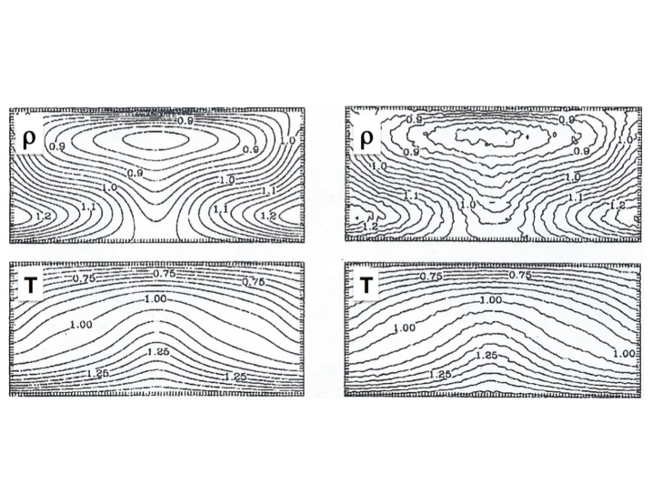
Figure 6: Rayleigh-Bénard rolls simulated with finite differences (left) and with SPAM (right) for a Rayleigh number of 10000. Upper panels are density contours and the lower panels are temperature contours. The temperatures at the top and bottom are respectively, 0.5 and 1.5 . The overall density is 1.0. The thermal diffusivity and kinematic viscosity are both chosen equal to 0.4 .

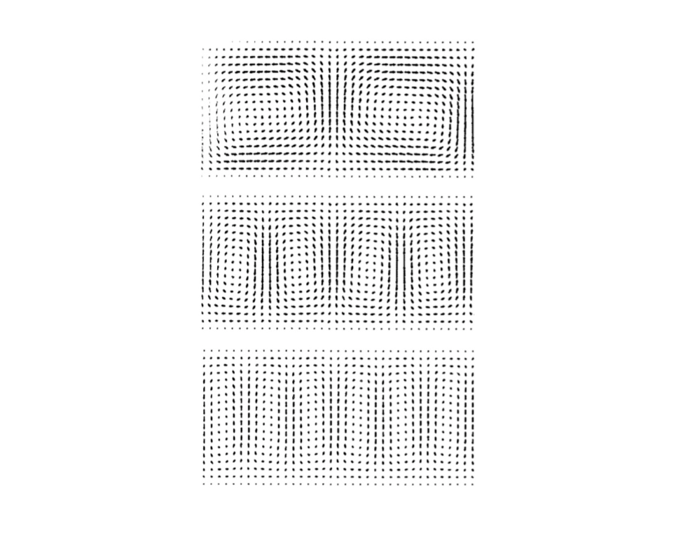
Figure 7: Two-roll, four-roll, and six-roll stationary flows for a two-dimensional ideal gas with $R=40,000$ and Prandtl number unity. Fully stationary two-roll solutions and four-roll solutions were obtained for meshes with 36x18, 72x36 and 144x72 nodes. The larger meshes show also six-roll solutions.

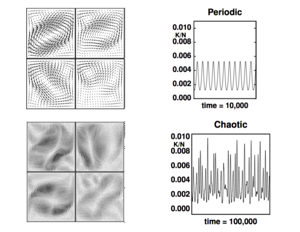
Figure 8: Morphology changes for high Rayleigh numbers. Harmonic morphology ( Top left ) of Rayleigh-Bénard rolls for a Rayleigh number of 160000. This solution uses an $80\times 80$ computational grid . Times shown are at one-eight of a perod. Chaotic morphology ( Bottom left ) for a Rayleigh number of 800000 using a $160\times 160$ computational grid. Time interval between the snapshots is 1000. The corresponding kinetic energies per particle are shown on the right side of the figure. See Section 4.11.2 of the fifth book of six shown in Figure 2.

With Harald and Vic Castillob14 ; b15 we used the motion-equation isomorphism to study the expansion of an ideal-gas fluid into a periodic volume four times larger than the original. See Figure 4. Our goal was better to understand the entropy increase associated with the expansion process, $Nk\ln(4)$ , where $k$ is Boltzmann’s constant. The ( equilibrium only ! ) entropy for the two-dimensional ideal gas is just $S=Nk\ln(e/\rho)$ .

Figure 4 shows five stages in the expansion process. At the top we see the particle locations. Below are the density and the kinetic energy. The white regions are above average and the black below. Three very significant points of interest were clarified by these simulations : [ 1 ] Equilibrium occurs quickly, in a time on the order of a sound traversal time; [ 2 ] The kinetic energy field, which contributes to the local energy and entropy, needs to be measured relative to the local stream velocity; and [ 3 ] Entropy must be evaluated using the local energy ( including the local fluctuating kinetic energy ) rather than the laboratory-frame energy. This last point becomes clear on looking at the time dependence of the two kinetic-energy calculations. Entropy increase ( in isentropic expansions ) doesn’t occur until the gas contacts its periodic images and begins the dissipation of mass motion into heat. See Figure 5 . The free expansion problemb14 ; b15 is particularly challenging for finite-element approaches due to its severe shear deformation and demonstrates the ability of SPAM to deal with interesting fluid mechanics problems. The simplicity of SPAM and its computer implementation make it an ideal teaching tool.

II.3 Rayleigh-Bénard Convection with SPAM

Another SPAM application is Rayleigh-Bénard convectionb16 ; b17 ; b18 . A fluid heated from below and subject to a gravitational field can exhibit several morphologies, depending upon the dimensionless Rayleigh Number. Again we choose a two-dimensional ideal gas. Here the system height is $H$ and the gravitational field strength is chosen consistent with constant density, $g=(k\Delta T/H)$ . The top-to-bottom temperature difference $\Delta T$ is equal to the mean temperature. The Rayleigh Number is ${\cal R}=(gH^{3}/\nu D)=10000$ . Here $\nu$ and $D$ are the kinematic viscosity and the thermal diffusivity. In Oyeon Kum’s PhD work he compared simulations with straightforward-but-tedious Eulerian continuum mechanics to SPAM. See Figure 6 for a two-roll solution which is stable at ${\cal R}=10000$ . At a higher value of the Rayleigh number, 40000 , three different stationary solutions of the continuum equations occurb17 ; b18 . See Figure 7.

Though maximum entropy or minimum entropy production have been touted as useful concepts in defining stability these examples show that there is no meaningful way to distinguish the relative stability ( as in thermodynamic phase stability ) of the different roll patterns. As the Rayleigh Number is increased through 90,000 the rolls begin regular vertical “harmonic” oscillations. Between 150,000 and 250,000 there are two separate solutions of the motion equations, one regular and harmonic, the other chaotic. See Figure 8. The harmonic solution transports heat a bit more efficiently than does its chaotic brotherb18 .

II.4 Lyapunov Instability and the Second Law of Thermodynamics

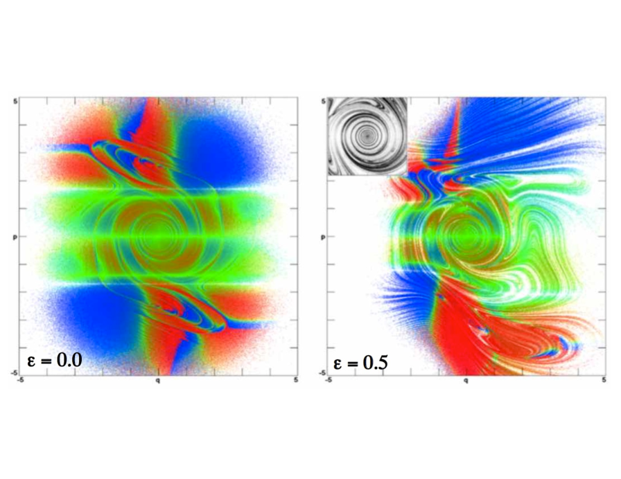
Figure 9: Penetrations of the $(\ q,p,0\ )$ plane for the chaotic and ergodic 0532 Model using an adaptive fourth-order Runge-Kutta integration with a timestep $dt\simeq 0.001$ . The red and blue points correspond to maximum and minimum values of the local Lyapunov exponent. The equilibrium $(\ \zeta=0\ )$ cross section at the left shows inversion symmetry, corresponding to viewing the oscillator in a mirror. The lack of symmetry about the horizontal $(\ p=0\ )$ axis shows that the exponents depend upon the past rather than the future. The nonequilibrium section ( $\epsilon=0.50$ ) shown to the right displays no symmetry at all and is multifractal. The black-and-white inset shows the cross-sectional density in the $2\times 2$ central region of the phase-plane section. $T=1+\epsilon\tanh(q)$ .

On the microscopic side our Lyapunov spectra project with Harald led us to dozens of studies of the effect of nonequilibrium conditions on the spectrumb19 . “Color” conductivity, where half the particles are accelerated to the right and the rest to the left, provided a particularly clear exampleb19 . Harald and Bill pointed out the simple shift of the Lyapunov spectrum in 1987b19 ; b20 . The Lyapunov spectrum of instability exponents shifts to more negative values with the sum of all exponents equal to the rate at which entropy is extracted from the system by deterministic thermostat forces. Similar results were obtained for a variety of shear flows and heat flows in systems with a variety of boundary conditions.

In every case nonequilibrium steady states occupy zero-volume fractal attractors in phase space ( meaning that the total volume of the cells in phase space containing any given fraction of the measure goes to zero as the small-cell limit is approached ). This fact demonstrates the extreme rarity of nonequilibrium states. The time reversibility of the motion equations shows that the dynamically unstable repellor is likewise of zero volume. The symmetry breaking revealed by these simulations shows that only those flows satisfying the Second Law of Thermodynamics are observableb20 .

Exactly the same mechanism for irreversibility from reversible motion equations can be seen in small systems. Even a single harmonic oscillator, exposed to a variable temperature $T(q)=1+\epsilon\tanh(q)$ can generate a chaotic heat flow and concentrate its stationary distribution on a fractal strange attractor. The “0532 Model”, which Bill mentionedb21 , incorporates “weak” control of $\langle\ (p^{2}/T)\ \rangle$ and $\langle\ (p^{4}/T^{2})\ \rangle$ and provides an ergodic canonical distribution for the harmonic oscillator, enforced by a single thermostat variable $\zeta$ :

$$\dot{q}=p\ ;\ \dot{p}=-q-\zeta[\ 0.05p+0.32(p^{3}/T)\ ]\ ;\ \dot{\zeta}=0.05[\ (p^{2}/T)-1\ ]+0.32[\ (p^{4}/T^{2})-3(p^{2}/T)\ ]\ .$$

Bill showed the stationary phase-space cross section for $(\ \epsilon=0\ )$ . Here Figure 9 shows the flux through the $(\ \zeta=0\ )$ phase-space plane for both the equilibrium flow and a nonequilibrium $(\ \epsilon=0.5\ )$ flow. The fractal character of the nonequilibrium section is clear. Notice also the symmetry breaking. Time reversal breaks the symmetry of the local Lyapunov exponent ( indicated by color ) as well as the mirror symmetry present at equilibrium but absent at nonequilibrium. In the nonequilibrium case the phase flow is from a repellor identical to the attractor except for the signs of $p$ and $\zeta$ . It is also the case that the rate of entropy production for the thermostated oscillator is equal to the rate of shrinkage of the phase volume $\otimes$ :

$$(\dot{S}/k)=\zeta[\ 0.05(p^{2}/T)+0.32(p^{4}/T^{2})\ ]\ ;\ (\dot{\otimes}/\otimes)=-\zeta[\ 0.05+0.96(p^{2}/T)\ ]$$

This is because the time average $\langle\ \zeta\dot{\zeta}\ \rangle\equiv 0$ implies that

$$\langle\ 0.05\zeta[\ (p^{2}/T)-1\ ]+0.32\zeta[\ (p^{4}/T^{2})-3(p^{2}/T)\ ]\rangle=0\ ,$$

or

$$\langle\ \zeta[\ 0.05(p^{2}/T)+0.32(p^{4}/T^{2})\ ]\ \rangle=\langle\ \zeta[\ 0.05+0.96(p^{2}/T)\ ]\ \rangle\ ,$$

so that the entropy production measured by the external thermostat is, when time averaged, precisely equal to the loss rate of Gibbs’ entropy in the nonequilibrium steady state.

Liouville’s Theorem turned out to be the most useful tool in understanding these ideasb9 . This flow equation for thermostated systems describes the phase-volume loss in terms of the friction coefficients imposing nonequilibrium constraints and in terms of the Lyapunov spectrum. Stationary flows satisfying the Second Law of Thermodynamics correspond to strange attractors, with shrinking phase volume. Flows violating the Law are both hard to find ( in the sense that they occupy zero phase volume ) and dynamically unstable ( in the sense that they have a positive unstable Lyapunov sum ) providing a mechanical analog for the Second Law of Thermodynamics directly from a determinstic time-reversible mechanics. Let us look at one particular manybody case, the $\phi^{4}$ model, which is both simple and profound.

II.5 The $\phi^{4}$ Model for Chaos and Fourier Heat Conduction

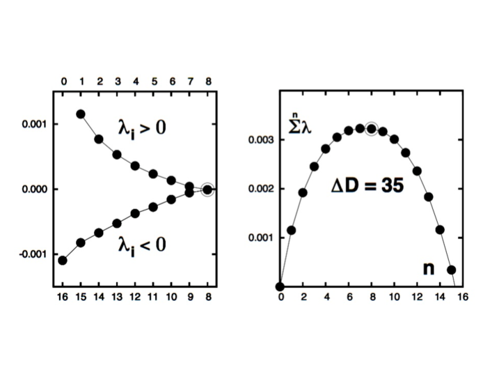
Figure 10: Lyapunov exponents ( left ) and their sums (right ), for a 24-particle $\phi^{4}$ chain with “cold” temperature $0.003$ and “hot” temperature $0.027$ . The dimensionality of the phase-space attractor is only 15 while the dimensionality of the entire phase space is 50.

Aoki and Kusnezov emphasized the utility of the $\phi^{4}$ model for statistical mechanics and explored its chaos and heat conductivity. It is a model of simplicityb23 ; b24 . Nearest-neighbor particles are joined by Hooke’s-Law springs. Each particle is also tethered to its lattice site with a quartic tether. The $\phi^{4}$ model Hamiltonian has kinetic, tether, and harmonic contributions :

$${\cal H}={\cal H}_{K}+{\cal H}_{t}+{\cal H}_{H}=\sum_{i}[\ (p_{i}^{2}/2)+(q_{i}^{4}/4)\ ]+\sum_{i<j}(q_{ij}^{2}/2)\ .$$

At low temperature there is no heat conductivity as energy can travel through a harmonic chain at the speed of sound. At high temperature there is no heat conductivity because the chain behaves as a system of independent quartic oscillators. But it turns out that the useful range of energies where the chain exhibits Fourier conductivity extends over about nine useful orders of magnitude in between !

In 2002 Harald and Bill studied the family of two-dimensional $\phi^{4}$ crystals ranging in size from $4\times 4$ to $12\times 12$ with boundary temperatures of 0.001 and 0.009. A fit to the data established that the dimensionality loss approaches 43 in the large-system limit while the phase space coordinates associated with thermostating are 5 for each thermostated particleb25 .

The one-dimensional case is more dramatic. In our most recent book we provided two more examples of largescale dimensionality loss using temperatures of 0.003 and 0.027. We found that the dimensionality of a 24-particle attractor in its 50-dimensional phase space was about 15. See Figure 10 . A 36-particle attractor in its 74-dimensional phase space had an attractor dimensionality of about 30. By 2005 we had a good understanding of many such simple models that illustrated the correspondence between microscopic fractal Lyapunov-unstable systems and phenomenological macroscopic fluid mechanics.

III Our Ongoing Working Vacation in Ruby Valley Nevada

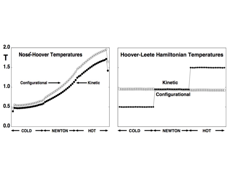
Figure 11: Kinetic and configurational temperature profiles for a 60-particle $\phi^{4}$ chain with the configurational temperatures shown as open circles. The temperatures on the left are solutions for the Nosé-Hoover equations of motion. The particle temperatures are averages over a billion-timestep simulation with $dt=0.01$ using a fourth-order Runge-Kutta integrator. Simulations with longer chains are in agreement with Aoki and Kusnezov’s work b23 ; b24 . The temperatures on the right correspond to using the Hoover-Leete Lagrangian/Hamiltonian thermostat to maintain the kinetic energies of the 20-particle cold and hot regions. Despite the successful thermostating of the reservoirs there is no heat flow. The Hoover-Leete configurational temperatures are nearly constant, and are equilibrated with the 20 Newtonian particles in the center of the $\phi^{4}$ chain. This simulation included a billion timesteps with $dt=0.001$ .

Bill spent much of my last “work” year in Livermore ( 2005 ) building us a new home in Ruby Valley just a couple of miles from the crest of the Ruby Mountains. Ruby Valley is a close-knit ranching community in northeastern Nevada. The cows, mostly Aberdeen Angus, outnumber the people by orders of magnitude and the telephone “book” is a single page, distributed annually at Christmas along with copies of a Christmas Card from each valley Family. Communication is vital to research. With airplanes and the internet we have continued our active research life in Ruby Valley. The cooperative and supportive nature of science is clear to us as we number our collaorators at well over 100 with at least that many more colleagues. Heat flow, ergodicity, chaos, and shockwaves have been our main research activities in Ruby Valley, along with related trips to Austria, Australia, England, Japan, Mexico, Poland, Russia, and Spainb26 ; b27 .

III.1 Hamiltonian Thermostats Do Not Promote Heat Flow

One of our earliest findings in Ruby Valley illustrates a shortcoming of Hamiltonian mechanics. It cannot describe steady heat flow. We happened on this finding in 2007b28 and revisited it in 2013b29 in response to unjustified claims for a “Hamiltonian thermostat” which turned out to be misleading and worthless. We have favored deterministic thermostating and the kinetic definition of temperature ever since Bill Ashurst’s work in the early 1970s. We thought it would be instructive to compare heat transport with the simple Nosé-Hoover thermostat to heat transport with straightforward Hamiltonian thermostats.

We considered three varieties of Hamiltonian thermostatsb30 , Nosé’s, which reproduces the entire canonical distribution, and two Lagrange-multiplier approaches leading to Hamiltonians which constrain the kinetic or the configurational temperatures of selected degrees of freedom. We found generally that Hamiltonian mechanics is incompatible with heat flow. If a cold thermostat extracts heat while a hot thermostat provides it, both at the same rate $\dot{Q}$ the system’s steady-state entropy change is negative ! :

$$\dot{S}=-(\dot{Q}/T_{\rm cold})+(\dot{Q}/T_{\rm hot})\simeq-(\dot{Q}\Delta T/T^{2})<0\ .$$

Here $\dot{Q}>0$ is the ( time-averaged ) rate at which heat flows both in and out of the system. Gibbs’ relation linking entropy to phase volume $S=k\ln(\otimes)$ suggests that any steady heat flow implies a loss of phase volume and is incompatible with Liouville’s Theorem. So the question is : What actually happens if the two heat reservoirs are modelled by Hamiltonian mechanics ? To find out we tried connecting several types of Hamiltonian thermostats to a Newtonian system in a sandwich fashion. The thermostats considered included : [ 1 ] Nosé’s original Hamiltonianb7 ; b8 , [ 2 ] the “Hoover-Leete” Hamiltonianb30 which constrains the kinetic energy to a fixed constant :

$${\cal H}_{HL}=2\sqrt{K(p)K(\dot{q})}-K(\dot{q})+\Phi\longrightarrow\dot{q}=p\sqrt{K(\dot{q})/K(p)}\longrightarrow K(\dot{q})\ {\rm constant}\ ,$$

and [ 3 ] a Hamiltonian which constrains the configurational temperature to a fixed constant. The configurational temperatureb31 folows from an integration by parts in the canonical ensemble:

$$\int(\nabla{\cal H})^{2}e^{-{\cal H}/kT}dq=kT\int\nabla^{2}{\cal H}e^{-{\cal H}/kT}dq\rightarrow kT=\frac{\langle\ (\nabla{\cal H})^{2}\ \rangle}{\langle\ \nabla^{2}{\cal H}\ \rangle}\ .$$

An extremely interesting thing happens when any one of these three Hamiltonian thermostats is applied to the $\phi^{4}$ heat-transfer problem. There is no heat flow ! Figure 11 illustrates a typical case, with the thermostated kinetic temperature in the hot and cold regions having the specified cold and hot values but with no current at all flowing through the Newtonian regions separating the two reservoirs. These problems make the point that any nonequilibrium simulation of heat flow with molecular dynamics is necessarily intrinsically nonHamiltonian. This conclusion is surprising, as was also the fractal nature of nonequilibrium distribution functions which came to light some thirty years ago in low-dimensional simulations of nonequilibrium transport in phase spaces of three or four space dimensions.

III.2 Shockwaves Revisited

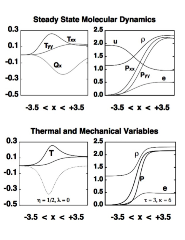
Figure 12: Molecular dynamics profiles (top) of mechanical and thermal variables generated with Lucy’s one-dimensional weight function $w(r<h=3)=(5/12)[\ 1+r\ ][\ 1-(r/3)\ ]^{3}$ . Mechanical and thermal variables (bottom) for a one-dimensional shockwave using the triangular-lattice “cold” curve, an allocation of the work and heat to $T_{xx}$ , and a tensor thermal conductivity with a thermal relaxation time of 3 . For details see Reference 27.

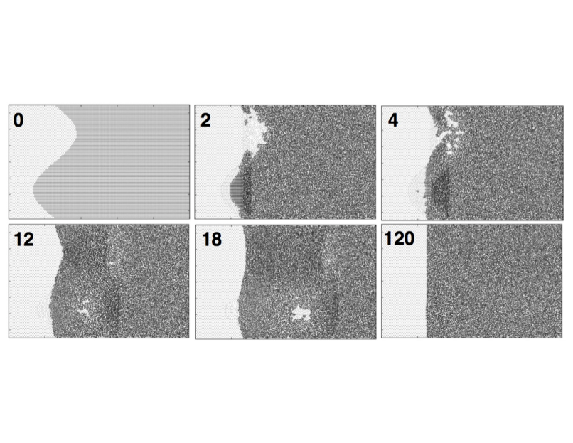
Figure 13: Evolution of a sinusoidal shockwave toward planarity. Snapshots distinguish particles with lower and higher densities than average. The window shown has length 100 with a periodic vertical height of $40\sqrt{3}$ . “Cold” stress-free material at the left has the close-packed triangular-lattice structure with a nearest-neighbor spacing of unity. “Hot” fluid at the right has twice that density. Particle motion is left-to-right with input speed twice the hot-fluid exit speed. Snapshot times appear in the upper left corners. Notice the low-density tensile waves in the third, fourth, and fifth frames. The pair potential is short-ranged : $\phi(r<1)=(10/\pi)(1-r)^{3}$ . The window shown moves at the shock velocity.

Bill’s early work on shockwaves was published in the Fall of 1967 in a summary of work at the Livermore Laboratory presented by Bill’s group leader Russ Duff at a meeting on the “Behavior of Dense Media Under High Dynamic Pressure” in Parisb32 . Ten years later Klimenko and Dremin published dynamical studiesb33 of two dense-fluid shockwaves for a model of argon. Ten years after that Brad Holian and Galen Straub at Los Alamos collaborated with Bill and Bill Moran to study a 400-kilobar shockwave in a model of argon, just below the pressure and temperature at which the fluid ionizesb34 . Thirty years later with Paco Uribeb26 ; b27 we carried out studies confronting a detailed model capable of matching the physical effects observed with molecular dynamics : [ 1 ] a large disparity between the longitudinal and transverse temperatures, [ 2 ] a time delay in the response of stress to strain and heat flux to a thermal gradient, and [ 3 ] a partition of heat and work into separate longitudinal and transverse components. These features are capable of describing the far-from-equilibrium states found in strong fluid shockwaves.

In correlating the results of molecular dynamics simulations with continuum models the smooth-particle averaging is invaluable. With SPAM averaging it was possible to establish the stability of planar shockwaves in two-dimensional systems as is shown in Figure 13. Throughout we have observed marked differences between the longitudinal and transverse temperatures as well as a time delay between the strain rate and the shear stress and between the temperature gradient(s) and the heat flux. With Paco Uribe in Mexico we were able to formulate and implement a detailed model capable of describing all of these effects. It is interesting that unless the delay time is brief, on the order of a collision time, the constitutive model becomes unstable.

III.3 Thermostats and India

In 2014 Bill received an interesting paper to review for The Journal of Chemical Physicsb35 . The authors, Baidurya Bhattacharya and his student Puneet Patra had the clever idea of thermostating both the kinetic and the configurational temperatures simultaneously. Bill thought this was a fine idea and wrote to them that he enjoyed their paper and was looking forward to its publication. The rapid-fire emails that followed soon led to the appearance of Baidurya in Ruby Valley for a visit, and then in 2015 to a visit with his Family, which makes regular trips to the United States in the summers. This led to a very productive collaboration and friendship.

We’ll be traveling to Kharagpur in December for some lectures at Professor Bhattacharya’s Institute, which we hope will turn out to be yet another book. This meeting led, though indirectly, to solving a problem that had puzzled Bill for 30 years : how to thermostat an ergodic canonical harmonic oscillator with a single thermostat variable. The Patra-Bhattacharya idea led first to simultaneous weak control of coordinates and momenta and finally to weak control of two kinetic-energy moments. Several specific examples proved ergodicity for the oscillator and the simple pendulum, but not ( so far ) for the quartic potential. This same work also led us into collaborations with Clint Sprott ( University of Wisconsin-Madison ), a wonderful colleague who has furnished many stimulating ideas as well as his graphical expertise which is illustrated here in Figure 9.

III.4 Moral

We are grateful to you all for your support, collaborations, friendship, and love over the years. Thanks for your attention to our reminiscences. Bill specially wants to thank Berni Alder for his participation here and for his extending a helping hand in so many ways that were crucial to the good life Bill and Carol have enjoyed so far. We urge those of you who are younger to reflect on your good fortune in being a part of our progress in understanding the world around us. Finally, we offer our thanks to Karl Travis and Fernando Bresme for their thoughtfulness and skill in organizing this meeting at Sheffield: “Advances in Theory and Simulation of Nonequilibrium Systems”.

References

- (1) W. G. Hoover, C. G. Hoover, and H. A. Posch, “Lyapunov Instability of Pendula, Chains and Strings”, Physical Review A 41, 2999-3004 (1990).
- (2) W. G. Hoover, Computational Statistical Mechanics (Elsevier, Amsterdam, 1991).
- (3) W. G. Hoover, A. J. De Groot, C. G. Hoover, I. F. Stowers, T. Kawai, B. L. Holian, T. Boku, S. Ihara, and J. Belak, “Large-Scale Elastic-Plastic Indentation Simulations via Molecular Dynamics”, Physical Review A 42, 5844-5853 (1990).
- (4) J. S. Kallman, W. G. Hoover, C. G. Hoover, A. J. De Groot, S. Lee, and F. Wooten, “Molecular Dynamics of Silicon Indentation”, Physical Review B 47, 7705-7709 (1993).
- (5) J. S. Kallman, A. J. De Groot, C. G. Hoover, W. G. Hoover, S. M. Lee, and F. Wooten, “Visualization Techniques for Molecular Dynamics”, IEEE Computer Graphics and Applications 15, 72-77 (November, 1995).
- (6) H. J. M. Hanley, Nonlinear Fluid Behavior, Proceedings of a 1982 Conference in Boulder, Colorado, published as Physica 118A, 1-454 (1983).
- (7) S. Nosé, “A Molecular Dynamics Method for Simulations in the Canonical Ensemble”, Molecular Physics 52, 255-268 (1984).
- (8) S. Nosé, “A Unified Formulation of the Constant Temperature Molecular Dynamics”, The Journal of Chemical Physics 81, 511-519 (1984).
- (9) W. G. Hoover, “Canonical Dynamics: Equilibrium Phase-Space Distributions”, Physical Review A 31, 1695-1697 (1985).
- (10) G. Ciccotti and W. G. Hoover, Molecular Dynamics Simulations of Statistical Mechanical Systems, Proceedings of the 1985 Enrico Fermi International School of Physics at Varenna (Elsevier, New York, 1986), 622 pages.
- (11) B. L. Holian, W. G. Hoover, and H. A. Posch, “Second-Law Irreversibility of Reversible Mechanical Systems” = “Resolution of Loschmidt’s Paradox: the Origin of Irreversible Behavior in Reversible Atomistic Dynamics”, Physical Review Letters 59, 10-13 (1987).
- (12) L. B. Lucy, “A Numerical Approach to the Testing of the Fission Hypothesis”, Astronomical Journal 82, 1013-1024 (1977).
- (13) J. J. Monaghan, “Smoothed Particle Hydrodynamics”, Annual Review of Astronomy and Astrophysics 30, 543-574 (1992).
- (14) Wm. G. Hoover and H. A. Posch, “Entropy Increase in Confined Free Expansions via Molecular Dynamics and Smooth-Particle Applied Mechanics”, Physical Review E 59, 1770-1776 (1999).
- (15) Wm. G. Hoover, H. A. Posch, V. M. Castillo, and C. G. Hoover, “Computer Simulation of Irreversible Expansions via Molecular Dynamics, Smooth Particle Applied Mechanics, Eulerian, and Lagrangian Continuum Mechanics”, Journal of Statistical Physics 100, 313-326 (2000).
- (16) O. Kum, W. G. Hoover, and H. A. Posch, “Viscous Conducting Flows with Smooth-Particle Applied Mechanics”, Physical Review E 52, 4899-4908 (1995).
- (17) V. M. Castillo, Wm. G. Hoover, and C. G. Hoover, “Coexisting Attractors in Compressible Rayleigh-Bénard Flow”, Physical Review E 55, 5546-5550 (1997).
- (18) V. M. Castillo and Wm. G. Hoover, “Entropy Production and Lyapunov Instability at the Onset of Turbulent Convection”, Physical Review E 58, 7350-7354 (1998).
- (19) W. G. Hoover and H. A. Posch, “Direct Measurement of Equilibrium and Nonequilibrium Lyapunov Spectra”, Physics Letters A 123, 227-230 (1987).
- (20) H. A. Posch and W. G. Hoover, “Chaotic Dynamics in Dense Fluids”, Liquids of Small Molecules, Proceedings of a Conference at Santa Trada, Calabria, Italy, presented on 22 September 1987 and available in the book of abstracts published by the European Physical Society.
- (21) P. K. Patra, J. C. Sprott, W. G. Hoover and C. G. Hoover, “Deterministic Time-Reversible Thermostats : Chaos, Ergodicity, and the Zeroth Law of Thermodynamics”, Molecular Physics 113, 2863-2872 (2015).
- (22) K. Aoki and D. Kusnezov, “Bulk Properties of Anharmonic Chains in Strong Thermal Gradients: Nonequilibrium Theory”, Physics Letters A 265, 250-256 (2000).
- (23) K. Aoki and D. Kusnezov, “Nonequilibrium Steady States and Transport in the Classical Lattice Theory”, Physics Letters B 477, 348-354 (2000).
- (24) H. A. Posch and W. G. Hoover, “Large-System Phase-Space Dimensionality Loss in Stationary Heat Flows”, Physica D 187, 281-293 (2004).
- (25) W. G. Hoover and C. G. Hoover, Simulation and Control of Chaotic Nonequilibrium Systems (World Scientific, Singapore, 2015).
- (26) W. G. Hoover, C. G. Hoover, and F. J. Uribe, “Flexible Macroscopic Models for Dense-Fluid Shockwaves: Partitioning Heat and Work; Delaying Stress and Heat Flux; Two-Temperature Thermal Relaxation”, Proceedings of the International Summer School Conference: “Advanced Problems in Mechanics-2010” organized by the Institute for Problems in Mechanical Engineering of the Russian Academy of Sciences in Mechanics and Engineering under the patronage of the Russian Academy of Sciences = arXiv 1005.1525 (2010).
- (27) F. J. Uribe, W. G. Hoover, C. G. Hoover, “Maxwell and Cattaneo’s Time-Delay Ideas Applied to Shockwaves and the Rayleigh-Bénard Problem”, Computational Methods in Science and Technology 19, 5-12 (2013).
- (28) Wm. G. Hoover and C. G. Hoover, “Hamiltonian Dynamics of Thermostated Systems: Two-Temperature Heat-Conducting Chains”, Journal of Chemical Physics 126, 164113 (2007).
- (29) W. G. Hoover and C. G. Hoover, “Hamiltonian Thermostats Fail to Promote Heat Flow”, Communications in Nonlinear Science and Numerical Simulation 18, 3365-3372 (2013).
- (30) T. Leete, The Hamiltonian Dynamics of Constrained Lagrangian Systems (Master’s Thesis, West Virginia University, 1979).
- (31) K. P. Travis and C. Braga, “Configurational Temperature Control for Atomic and Molecular Systems”, The Journal of Chemical Physics 128, 014111 (2008) = arXiv 0709.1575.
- (32) R. E. Duff, W. H. Gust, E. B. Royce, M. Ross, A. C. Mitchell, R. N. Keeler, and W. G. Hoover, “Shockwave Studies in Condensed Media”, in Behavior of Dense Media Under High Dynamic Pressures (Gordon and Breach, New York, 1968).
- (33) V. Y. Klimenko and A. N. Dremin, “Structure of Shockwave Front in a Liquid” in Detonation, Chernogolovka, edited by O. N. Breusov et alii (Akademiya Nauk, Moscow, SSSR, 1978), pages 79-83.
- (34) B. L. Holian, W. G. Hoover, B. Moran, and G. K. Straub, “Shockwave Structure via Nonequilibrium Molecular Dynamics and Navier-Stokes Continuum Mechanics”, Physical Review A 22, 2798-2808 (1980).
- (35) P. K. Patra and B. Bhattacharya, “A Deterministic Thermostat for Controlling Temperature Using All Degrees of Freedom”, The Journal of Chemical Physics 140, 064106 (2014).