Understanding the internal structures of the $X(4140)$, $X(4274)$, $X(4500)$ and $X(4700)$

Abstract

We investigate the newly observed $X(4500)$ and $X(4700)$ based on the diquark-antidiquark configuration within the framework of QCD sum rules. Both of them may be interpreted as the $D$-wave $cs\bar{c}\bar{s}$ tetraquark states of $J^{P}=0^{+}$, but with opposite color structures, which is remarkably similar to the result obtained in Ref. Chen:2010ze that the $X(4140)$ and $X(4274)$ can be both interpreted as the $S$-wave $cs\bar{c}\bar{s}$ tetraquark states of $J^{P}=1^{+}$, also with opposite color structures. However, the extracted masses and these suggested assignments to these $X$ states do depend on these running quark masses where $m_{s}(2\mbox{ GeV})=95\pm 5$ MeV and $m_{c}(m_{c})=1.23\pm 0.09$ GeV. As a byproduct, the masses of the hidden-bottom partner states of the $X(4500)$ and $X(4700)$ are extracted to be both around 10.64 GeV, which can be searched for in the $\Upsilon\phi$ invariant mass distribution.

Introduction.—It is well known that our world is made from nucleons and electrons while nucleons are made from quarks and gluons. However, we still know little (not enough) on how quarks and gluons compose nucleons, which can be better understood by exploring exotic matter beyond the conventional quark model, such as glueballs, hybrids and multiquark states, etc. Agashe:2014kda ; Jaffe:2004ph ; Liu:2013waa ; Chen:2016qju . With significant experimental progress over the past decade, lots of multiquark candidates have been observed, including dozens of charmonium-like and bottomonium-like $XYZ$ states Agashe:2014kda and the hidden-charm pentaquark states $P_{c}(4380)$ and $P_{c}(4450)$ Aaij:2015tga . They are new blocks of QCD matter, and provide important hints to deepen our understanding of the non-perturbative quantum chromodynamics (QCD).

Very recently the LHCb Collaboration confirmed the $X(4140)$ and $X(4274)$ in the $J/\psi\phi$ invariant mass distribution and determined their spin-parity quantum numbers to be both $J^{P}=1^{++}$ lhcb . At the same time they investigated the high $J/\psi\phi$ mass region for the first time, where the results can be described as a nonresonant term plus two new $J^{P}=0^{++}$ resonances, named as the $X(4500)$ and $X(4700)$. Their masses and widths were measured to be:

$$X(4140):M=4146.5\pm 4.5^{+4.6}_{-2.8}\mbox{ MeV}\,,$$

$$~{}~{}~{}~{}~{}~{}~{}~{}~{}~{}~{}~{}~{}~{}\Gamma=83\pm 21^{+21}_{-14}\mbox{ MeV}\,,$$

$$X(4274):M=4273.3\pm 8.3^{+17.2}_{-3.6}\mbox{ MeV}\,,$$

$$~{}~{}~{}~{}~{}~{}~{}~{}~{}~{}~{}~{}~{}~{}\Gamma=56\pm 11^{+8}_{-11}\mbox{ MeV}\,,$$

$$X(4500):M=4506\pm 11^{+12}_{-15}\mbox{ MeV}\,,$$

$$~{}~{}~{}~{}~{}~{}~{}~{}~{}~{}~{}~{}~{}~{}\Gamma=92\pm 21^{+21}_{-20}\mbox{ MeV}\,,$$

$$X(4700):M=4704\pm 10^{+14}_{-24}\mbox{ MeV}\,,$$

$$~{}~{}~{}~{}~{}~{}~{}~{}~{}~{}~{}~{}~{}~{}\Gamma=120\pm 31^{+42}_{-33}\mbox{ MeV}\,.$$

The $X(4140)$ Aaltonen:2009tz and the $X(4274)$ Aaltonen:2011at were first reported by the CDF Collaboration in 2009 and 2011 respectively. Many theoretical explanations were proposed such as the $D_{s}^{*}\bar{D}_{s}^{*}$ and $D_{s}\bar{D}_{s0}(2317)$ molecular states Liu:2008tn ; Liu:2009ei ; Mahajan:2009pj ; Branz:2009yt ; Ding:2009vd ; Liu:2010hf ; Wang:2011uk ; Finazzo:2011he ; He:2011ed ; HidalgoDuque:2012pq , compact tetraquark states (diquark-antidiquark states) Stancu:2009ka ; Patel:2014vua , dynamically generated resonances Molina:2009ct ; Branz:2010rj , and coupled-channel effects Danilkin:2009hr ; vanBeveren:2009dc , etc.

Among these studies, the results obtained within the framework of QCD sum rules are significant  Chen:2010ze ; Albuquerque:2009ak ; Zhang:2009st ; Wang:2009ue ; Wang:2009ry , which method has been applied to studied many other multiquark candidates Chen:2006zh ; Chen:2015moa ; Chen:2016ymy . In 2010, Chen, et al. studied the vector and axial-vector charmonium-like states systematically in Ref.  Chen:2010ze , where they used the following two $J^{P}=1^{+}$ currents to perform QCD sum rule analyses ($a$ and $b$ are color indices):

$$J_{3\mu} = s^{T}_{a}C\gamma_{5}c_{b}(\bar{s}_{a}\gamma_{\mu}C\bar{c}^{T}_{b}+\bar{s}_{b}\gamma_{\mu}C\bar{c}^{T}_{a})$$

$$~{}~{}~{}~{}~{}~{}~{}~{}~{}~{}~{}~{}+s^{T}_{a}C\gamma_{\mu}c_{b}(\bar{s}_{a}\gamma_{5}C\bar{c}^{T}_{b}+\bar{s}_{b}\gamma_{5}C\bar{c}^{T}_{a})\,,$$

$$J_{4\mu} = s^{T}_{a}C\gamma_{5}c_{b}(\bar{s}_{a}\gamma_{\mu}C\bar{c}^{T}_{b}-\bar{s}_{b}\gamma_{\mu}C\bar{c}^{T}_{a})$$

$$~{}~{}~{}~{}~{}~{}~{}~{}~{}~{}~{}~{}+s^{T}_{a}C\gamma_{\mu}c_{b}(\bar{s}_{a}\gamma_{5}C\bar{c}^{T}_{b}-\bar{s}_{b}\gamma_{5}C\bar{c}^{T}_{a})\,,$$

which are constructed using diquark and antidiquark fields. There are altogether five diquark fields: $q^{T}_{a}Cq_{b}$, $q^{T}_{a}C\gamma_{5}q_{b}$, $q^{T}_{a}C\gamma_{\mu}q_{b}$, $q^{T}_{a}C\gamma_{\mu}\gamma_{5}q_{b}$ and $q^{T}_{a}C\sigma_{\mu\nu}q_{b}$ Chen:2006hy ; Chen:2007xr . Among them, the $S$-wave diquark fields $q_{a}^{T}C\gamma_{5}q_{b}$ and $q_{a}^{T}C\gamma_{\mu}q_{b}$ are favored Jaffe:2004ph ; Maiani:2004vq ; Kleiv:2013dta , which can be used to further construct the “good” and “bad” diquarks by demanding their color structure to be antisymmetric $[\mathbf{\bar{3}_{c}}]_{qq}$ (by simply adding a totally antisymmetric tensor $\epsilon^{abc}$) Jaffe:2004ph . The other three “worse” diquarks all contain $P$-wave components Jaffe:2004ph .

The current $J_{4\mu}$ defined in Eq. (Understanding the internal structures of the $X(4140)$, $X(4274)$, $X(4500)$ and $X(4700)$) has the antisymmetric color structure $[\mathbf{\bar{3}_{c}}]_{cs}\otimes[\mathbf{3_{c}}]_{\bar{c}\bar{s}}$. Hence, this interpolating current consists of one “good” diquark and one “bad” antidiquark, and is the most favored one among all the $J^{P}=1^{+}$ currents. Its extracted mass is $4.07\pm 0.10$ GeV Chen:2010ze , consistent with the experimental mass of the $X(4140)$ Agashe:2014kda . The current $J_{3\mu}$ defined in Eq. (Understanding the internal structures of the $X(4140)$, $X(4274)$, $X(4500)$ and $X(4700)$) consists of one similar diquark and one similar antidiquark, but having the symmetric color structure $[\mathbf{6_{c}}]_{cs}\otimes[\mathbf{\bar{6}_{c}}]_{\bar{c}\bar{s}}$. Hence, it is less favored but still better than other currents containing “worse ”diquarks Jaffe:2004ph . Its extracted mass is $4.22\pm 0.10$ GeV Chen:2010ze , consistent with the experimental mass of the $X(4274)$ Agashe:2014kda .

The P-wave vector tetraquark states were discussed extensively in Ref. Lebed:2016yvr . There also exist investigations of the scalar tetraquark states. In Refs. Albuquerque:2009ak ; Zhang:2009st ; Wang:2009ue ; Wang:2009ry three groups studied the scalar $D^{*}_{s}\bar{D}^{*}_{s}$ molecular state through the current composed of two vector meson fields

$$J_{D^{*}_{s}\bar{D}^{*}_{s}}(x)=\bar{c}_{a}(x)\gamma_{\mu}s_{a}(x)\bar{s}_{b}(x)\gamma^{\mu}c_{b}(x)\,.$$ (3)

Two of the three groups obtained similar results using $J_{D^{*}_{s}\bar{D}^{*}_{s}}$, $4.14\pm 0.09$ GeV  Albuquerque:2009ak and $4.13\pm 0.10$ GeV  Zhang:2009st . The extracted mass is $3.91\pm 0.10$ GeV with the $D_{s}\bar{D}_{s}$ current  Zhang:2009st

$$J_{D_{s}\bar{D}_{s}}(x)=\bar{c}_{a}(x)\gamma_{5}s_{a}(x)\bar{s}_{b}(x)\gamma_{5}c_{b}(x)\,.$$ (4)

The third group extracted a significantly larger mass $4.43\pm 0.16$ GeV Wang:2009ue ; Wang:2009ry , which is significantly larger than the $D_{s}^{*}\bar{D}_{s}^{*}$ threshold, 4.22 GeV.

The $X(4500)$ and $X(4700)$ have masses significantly larger than the $X(4140)$ and $X(4274)$ of $J^{P}=1^{+}$. They can be good candidates of the $D$-wave tetraquark states of $J^{P}=0^{+}$, whose possible angular momenta are $\{[cs]_{s=1}$ $[\bar{c}\bar{s}]_{s=1};L=S=2,J=0\}$. Hence, the “good” diquark of $S=0$ can not be used, but they can still be composed by the “bad” diquark of $S=1$, $\epsilon^{abc}q_{a}^{T}C\gamma_{\mu}q_{b}$. We also need the $P$-wave “bad” diquark field $\epsilon^{abc}q^{T}_{a}C\gamma_{\mu_{1}}D_{\mu_{2}}q_{b}$ and the $D$-wave “bad” diquark field $\epsilon^{abc}q^{T}_{a}C\gamma_{\mu_{1}}D_{\mu_{2}}D_{\mu_{3}}q_{b}$, as well as their partners having the symmetric color structure $[\mathbf{6_{c}}]_{qq}$.

In this work we will show that the $X(4500)$ and $X(4700)$ can be both interpreted as $D$-wave tetraquark states with the quark content $cs\bar{c}\bar{s}$ and $J^{P}=0^{+}$: the $X(4500)$ consists of one $D$-wave “bad” diquark and one $S$-wave “bad” antidiquark, having the antisymmetric color structure $[\mathbf{\bar{3}_{c}}]_{cs}\otimes[\mathbf{3_{c}}]_{\bar{c}\bar{s}}$; the $X(4700)$ consists of one similar $D$-wave diquark and one similar $S$-wave antidiquark, but having the symmetric color structure $[\mathbf{6_{c}}]_{cs}\otimes[\mathbf{\bar{6}_{c}}]_{\bar{c}\bar{s}}$.

These two interpretations are remarkably similar to those obtained in Ref. Chen:2010ze that the $X(4140)$ and $X(4274)$ can be both interpreted as $S$-wave tetraquark states with the quark content $cs\bar{c}\bar{s}$ and $J^{P}=0^{+}$: the $X(4140)$ consists of one $S$-wave “good” diquark and one $S$-wave “bad” antidiquark, having the antisymmetric color structure $[\mathbf{\bar{3}_{c}}]_{cs}\otimes[\mathbf{3_{c}}]_{\bar{c}\bar{s}}$; the $X(4274)$ consists of two similar $S$-wave diquarks, but having the symmetric color structure $[\mathbf{6_{c}}]_{cs}\otimes[\mathbf{\bar{6}_{c}}]_{\bar{c}\bar{s}}$.

To examine these interpretations, we investigate the bottom partner states of the $X(4500)$ and $X(4700)$, and extract their masses to be both around 10.64 GeV. We propose to search for them in the $\Upsilon\phi$ invariant mass distribution with the running of LHC at 13 TeV and forthcoming BelleII. If the above interpretations of the $X(4140)$, $X(4274)$, $X(4500)$ and $X(4700)$ are correct, their dual partner would be quite interesting, such as the $S$-wave scalar and the $D$-wave axial-vector $cs\bar{c}\bar{s}$ tetraquark states, consisting of two “bad” diquarks with both symmetric and antisymmetric color structures. All their related studies, both experimentally and theoretically, can deepen our understanding of the non-perturbative QCD. Especially, our present study can be helpful to improve our understanding of the internal structures of exotic hadrons.

Interpretation of the $X(4500)$ and $X(4700)$.—As the first step, we use the $S/P/D$-waves “axial-vector” diquarks of $S=1$ to construct the $D$-wave $cs\bar{c}\bar{s}$ tetraquark currents of $J^{P}=0^{+}$. There are two possible ways. One way is to use the combination of one $P$-wave diquark and one $P$-wave antidiquark:

$$J_{1\pm} = c_{a}^{T}C\gamma_{\mu_{1}}[D_{\mu_{3}}s_{b}](\bar{c}_{a}\gamma_{\mu_{2}}C[D^{\dagger}_{\mu_{4}}\bar{s}_{b}^{T}]\pm\bar{c}_{b}\gamma_{\mu_{2}}C[D^{\dagger}_{\mu_{4}}\bar{s}_{a}^{T}])$$ (5)

$$\times\left(g^{\mu_{1}\mu_{3}}g^{\mu_{2}\mu_{4}}+g^{\mu_{1}\mu_{4}}g^{\mu_{2}\mu_{3}}-g^{\mu_{1}\mu_{2}}g^{\mu_{3}\mu_{4}}/2\right)\,,$$

where $J_{1+}$ has the symmetric color structure $[\mathbf{6_{c}}]_{cs}\otimes[\mathbf{\bar{6}_{c}}]_{\bar{c}\bar{s}}$, and $J_{1-}$ has the antisymmetric color structure $[\mathbf{\bar{3}_{c}}]_{cs}\otimes[\mathbf{3_{c}}]_{\bar{c}\bar{s}}$; they both have $l_{cs}=l_{\bar{c}\bar{s}}=1$ and $s_{cs}=s_{\bar{c}\bar{s}}=1$, and their total momenta are $L=S=2$ and $J=0$.

The other way is to use the combination of one $D$-wave diquark and one $S$-wave antidiquark:

$$J_{2\pm} = c_{a}^{T}C\gamma_{\mu_{1}}[D_{\mu_{3}}D_{\mu_{4}}s_{b}](\bar{c}_{a}\gamma_{\mu_{2}}C\bar{s}_{b}^{T}\pm\bar{c}_{b}\gamma_{\mu_{2}}C\bar{s}_{a}^{T})$$ (6)

$$\times\left(g^{\mu_{1}\mu_{3}}g^{\mu_{2}\mu_{4}}+g^{\mu_{1}\mu_{4}}g^{\mu_{2}\mu_{3}}-g^{\mu_{1}\mu_{2}}g^{\mu_{3}\mu_{4}}/2\right)\,,$$

where $J_{2+}$ has the symmetric color structure $[\mathbf{6_{c}}]_{cs}\otimes[\mathbf{\bar{6}_{c}}]_{\bar{c}\bar{s}}$, and $J_{2-}$ has the antisymmetric color structure $[\mathbf{\bar{3}_{c}}]_{cs}\otimes[\mathbf{3_{c}}]_{\bar{c}\bar{s}}$; they both have $l_{cs}=2$, $l_{\bar{c}\bar{s}}=0$ and $s_{cs}=s_{\bar{c}\bar{s}}=1$, and their total momenta are also $L=S=2$ and $J=0$.

The $D$-wave tetraquark currents can also be constructed by using the $S/P/D$-waves mesonic fields,

$$J_{1}^{\prime} = \bar{c}_{a}\gamma_{\mu_{1}}[D_{\mu_{3}}s_{a}][D^{\dagger}_{\mu_{4}}\bar{s}_{b}]\gamma_{\mu_{2}}c_{b}$$

$$~{}~{}~{}\times\left(g^{\mu_{1}\mu_{3}}g^{\mu_{2}\mu_{4}}+g^{\mu_{1}\mu_{4}}g^{\mu_{2}\mu_{3}}-g^{\mu_{1}\mu_{2}}g^{\mu_{3}\mu_{4}}/2\right)\,,$$

$$J_{2}^{\prime} = \bar{c}_{a}\gamma_{\mu_{1}}[D_{\mu_{3}}D_{\mu_{4}}s_{a}]\bar{s}_{b}\gamma_{\mu_{2}}c_{b}$$

$$~{}~{}~{}\times\left(g^{\mu_{1}\mu_{3}}g^{\mu_{2}\mu_{4}}+g^{\mu_{1}\mu_{4}}g^{\mu_{2}\mu_{3}}-g^{\mu_{1}\mu_{2}}g^{\mu_{3}\mu_{4}}/2\right)\,.$$

These currents have the color structure $[\mathbf{1_{c}}]_{\bar{c}s}\otimes[\mathbf{1_{c}}]_{\bar{s}c}$. Moreover, the color-octet quark-antiquark pairs can also be used to construct the tetraquark currents having the hidden-color structure $[\mathbf{8_{c}}]_{\bar{c}s}\otimes[\mathbf{8_{c}}]_{\bar{s}c}$. We will not investigate such currents in the present study, but note that we can use the Fierz and color rearrangements to relate the local diquark-antiquark and dimeson currents (see Refs. Chen:2016qju ; Chen:2006hy ; Chen:2007xr for detailed discussions).

In the following we use the currents $J_{i\pm}$ ($i=1,2$) to study the $D$-wave $cs\bar{c}\bar{s}$ tetraquark states of $J^{P}=0^{+}$, denoted as $X$, using the method of QCD sum rules, which provides a model-independent method to study nonperturbative problems in strong interaction physics Shifman:1978bx ; Reinders:1984sr ; Nielsen:2009uh ; colangelo ; Narison:2002pw . We need to deal with the two derivative operators inside $J_{i\pm}$, which has been applied to study the $D$ and $F$-wave heavy-light mesons Zhou:2014ytp ; Zhou:2015ywa ; Chen:2011qu . $J_{i\pm}$ couples to $X$ through

$$\langle 0|J|X\rangle=f_{X}\,.$$ (9)

Then the two-point correlation function can be written as

$$\Pi(p^{2}) =i\int d^{4}xe^{ip\cdot x}\langle 0|T[J(x)J^{{\dagger}}(0)]|0\rangle\,,$$ (10)

which can be calculated in the QCD operator product expansion (OPE) up to certain order in the expansion, and then matched with a hadronic parametrization to extract information about $X$.

At the hadron level, Eq. (10) can be written as

$$\Pi(p^{2})={\frac{1}{\pi}}\int^{\infty}_{s_{<}}\frac{{\rm Im}\Pi(s)}{s-p^{2}-i\varepsilon}ds\,,$$ (11)

where $s_{<}$ is the physical threshold. We define its imaginary part as the spectral function $\rho(s)$, and evaluate it by inserting intermediate hadron states $\sum_{n}|n\rangle\langle n|$

$$\rho(s)\equiv\frac{1}{\pi}{\rm Im}\Pi(s) = \sum_{n}\delta(s-M^{2}_{n})\langle 0|\eta|n\rangle\langle n|{\eta^{\dagger}}|0\rangle$$ (12)

$$= f_{X}^{2}\delta(s-m_{X}^{2})+\mbox{continuum}\,,$$

where we only take into account the lowest-lying resonance $|X\rangle$, and $m_{X}$ and $f_{X}$ are its mass and coupling constant, respectively.

We can also evaluate the spectral density $\rho(s)$ at the quark and gluon level via the QCD operator product expansion. In this work we evaluate it up to dimension ten, including the perturbative term, the quark condensate $\langle\bar{s}s\rangle$, the gluon condensate $\langle g_{s}^{2}GG\rangle$, the quark-gluon mixed condensates $\langle g_{s}\bar{s}\sigma Gs\rangle$ and $\langle g_{s}\bar{s}\sigma Gs\rangle^{2}$. The full expressions are lengthy and will not be shown here. We have also calculated the condensates $\langle\bar{s}s\rangle^{2}$ and $\langle\bar{s}s\rangle\langle g_{s}\bar{s}\sigma Gs\rangle$, which can be important in sum rule studies Chen:2010ze . However, both of them vanish when the currents $J_{i\pm}$ ($i=1\cdots 2$) are used.

After performing the Borel transform at both the hadron and QCD levels, we can express the two-point correlation function as

$$\Pi^{(all)}(M_{B}^{2})\equiv\mathcal{B}_{M_{B}^{2}}\Pi(p^{2})=\int^{\infty}_{s_{<}}e^{-s/M_{B}^{2}}\rho(s)ds\,.$$ (13)

Then assuming the contribution from continuum states can be approximated well by the OPE spectral density above a threshold value $s_{0}$ (duality)

$$\Pi(s_{0},M_{B}^{2})=\int^{s_{0}}_{s_{<}}e^{-s/M_{B}^{2}}\rho(s)ds\,,$$ (14)

we finally arrive at the sum rule relation:

$$M^{2}_{X}(s_{0},M_{B}) = {\int^{s_{0}}_{s_{<}}e^{-s/M_{B}^{2}}\rho(s)sds\over\int^{s_{0}}_{s_{<}}e^{-s/M_{B}^{2}}\rho(s)ds}\,.$$ (15)

To perform numerical analysis, we use the following QCD parameters of quark masses and various QCD condensates Agashe:2014kda ; colangelo ; Narison:2002pw ; Eidemuller:2000rc ; Gimenez:2005nt ; Jamin:2002ev ; Ioffe:2002be ; Ovchinnikov:1988gk :

$$\langle\bar{q}q\rangle=-(0.24\pm 0.01)^{3}\mbox{ GeV}^{3}\,,$$

$$\langle\bar{s}s\rangle=(0.8\pm 0.1)\times\langle\bar{q}q\rangle\,,$$

$$\langle g_{s}^{2}GG\rangle=(0.48\pm 0.14)\mbox{ GeV}^{4}\,,$$

$$\langle g_{s}\bar{s}\sigma Gs\rangle=-M_{0}^{2}\times\langle\bar{s}s\rangle\,,$$ (16)

$$M_{0}^{2}=0.8\mbox{ GeV}^{2}\,,$$

$$m_{s}(2\mbox{ GeV})=95\pm 5\mbox{ MeV}\,,$$

$$m_{c}(m_{c})=1.23\pm 0.09\mbox{ GeV}\,,$$

in which $\overline{m}_{s}$ and $\overline{m}_{c}$ are the “running masses” of the strange and charm quarks in the $\overline{\rm MS}$ scheme. We note that there is an additional minus sign in mixed condensates due to the different definition of the coupling constant $g_{s}$ compared to that in Ref. Reinders:1984sr .

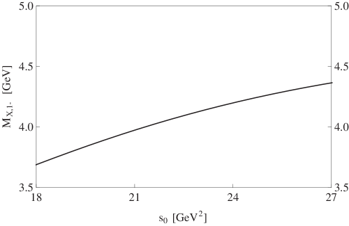
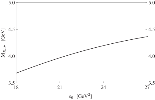
Figure 1: Variations of $M_{X}$ with respect to the threshold value $s_{0}$, when the Borel mass $M_{B}$ is fixed to be $M_{B}^{2}=2.0$ GeV², obtained using the currents $J_{1-}$ (left) and $J_{1+}$ (right).

There are two free parameters in Eq. (15): the threshold value $s_{0}$ and the Borel mass $M_{B}$. The QCD sum rule prediction of the hadron mass $M_{X}$ is only significant and reliable in suitable regions of the parameter space $(s_{0},M_{B}^{2})$.

First we fix $M_{B}^{2}=2.0$ GeV² and investigate the $s_{0}$ dependence. The mass curves obtained using $J_{1-}$ and $J_{1+}$ (consisting of one $P$-wave diquark and one $P$-wave antidiquark) are shown in Fig. 1. We find that their results are similar to each other, i.e., the evaluated masses $M_{X,1\pm}$ monotonically increase with $s_{0}$. We do not want conclude that this is “bad” sum rule results, but it seems difficult to extract the hadron mass $M_{X}$ using these two currents. Hence, we shall not discuss $J_{1-}$ and $J_{1+}$ any more.

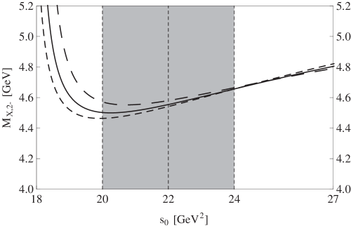
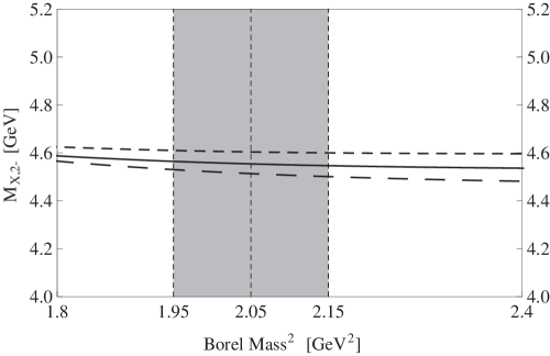
Figure 2: The variation of $M_{X}$ with respect to the threshold value $s_{0}$ (left) and the Borel mass $M_{B}$ (right), calculated using the current $J_{2-}$ of $J^{P}=0^{+}$. In the left figure, the long-dashed, solid and short-dashed curves are obtained by fixing $M_{B}^{2}=1.85$, $2.05$ and $2.25$ GeV², respectively. In the right figure, the long-dashed, solid and short-dashed curves are obtained for $s_{0}=21$, $22$ and $23$ GeV², respectively.

The results obtained using $J_{2-}$ and $J_{2+}$ (consisting of one $D$-wave diquark and one $S$-wave antidiquark) are also similar to each other but different from $J_{1\pm}$, i.e., the obtained masses $M_{X,2\pm}$ both have a mass plateau, where the $s_{0}$ dependence is the weakest Narison:1996fm ; Chen:2010ze . We use the current $J_{2-}$ as an example and show the mass curves in the left panel of Fig. 2 as a function of the threshold value $s_{0}$. We notice that the $s_{0}$ dependence is the weakest around $s_{0}\sim 20$ GeV², and the $M_{B}$ dependence is the weakest around $s_{0}\sim 24$ GeV². Accordingly, we choose the region $20$ GeV${}^{2}\leq s_{0}\leq 24$ GeV² as our working region, where the $s_{0}$ and $M_{B}$ dependence is both acceptable. This is our first criterion to determine $s_{0}$, i.e., the $s_{0}$ and $M_{B}$ stability.

After fixing $s_{0}$, we use two extra criteria to constrain the Borel mass $M_{B}$: a) to insure the convergence of the OPE series, we require that the mixed condensate $\langle g_{s}\bar{s}\sigma Gs\rangle$ be less than 30% to determine its lower limit $M_{B}^{min}$ (the contribution from the highest condensate $\langle g_{s}\bar{s}\sigma Gs\rangle^{2}$ is negligible, so we do not use it in this criterion):

$$\mbox{Convergence (CVG)}\equiv\left|\frac{\Pi_{\langle g_{s}\bar{s}\sigma Gs\rangle}(\infty,M_{B})}{\Pi(\infty,M_{B})}\right|\leq 30\%\,;$$ (17)

b) to insure that the one-pole parametrization in Eq. (12) is valid, we require that the pole contribution (PC) be larger than 20% to determine the upper limit on $M_{B}^{2}$:

$$\mbox{PC}\equiv\frac{\Pi(s_{0},M_{B})}{\Pi(\infty,M_{B})}\geq 20\%\,.$$ (18)

The small pole contribution is due to the large powers of $s$ in the spectral function (see other sum rule analyses for the six-quark state $d^{*}(2380)$ Chen:2014vha and the $F$-wave heavy mesons Zhou:2015ywa ).

Using these two criteria we obtain the working region of the Borel mass to be $1.95$ GeV${}^{2}<M_{B}^{2}<2.15$ GeV² for the current $J_{2-}$ with $s_{0}=22$ GeV² (there exist Borel windows only when $s_{0}\geq 22$ GeV²). The variation of $M_{X}$ with respect to the Borel mass $M_{B}$ is shown in the right panel of Fig. 2, where the mass curves are very stable not only inside this Borel window but also in a larger nearby area.

Together we obtain the working regions for the current $J_{2-}$ to be $20$ GeV${}^{2}\leq s_{0}\leq 24$ GeV² and $1.95$ GeV${}^{2}<M_{B}^{2}<2.15$ GeV², where $M_{X}$ can be extracted to be:

$$M_{X,2-}=4.55^{+0.19}_{-0.13}\mbox{ GeV}\,,$$ (19)

Here the central value corresponds to $M_{B}^{2}=2.05$ GeV² and $s_{0}=22$ GeV², and the uncertainty comes from the Borel mass $M_{B}$, the threshold value $s_{0}$, the strange and charm quark masses, and the various condensates. This value is consistent with the experimental mass of the $X(4500)$ lhcb , supporting it to be a $D$-wave $cs\bar{c}\bar{s}$ tetraquark state of $J^{P}=0^{+}$. It consists of one $D$-wave “bad” diquark and one $S$-wave “bad” antidiquark, having the antisymmetric color structure $[\mathbf{\bar{3}_{c}}]_{cs}\otimes[\mathbf{3_{c}}]_{\bar{c}\bar{s}}$.

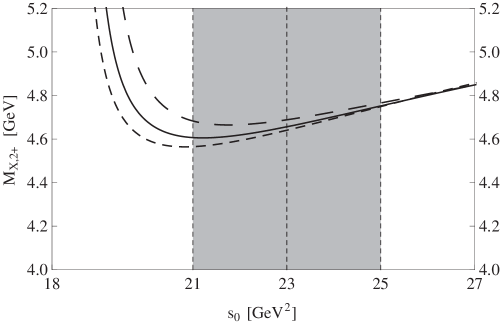
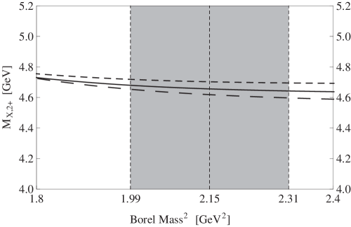
Figure 3: The variation of $M_{X}$ with respect to the threshold value $s_{0}$ (left) and the Borel mass $M_{B}$ (right), calculated using the current $J_{2+}$ of $J^{P}=0^{+}$. In the left figure, the long-dashed, solid and short-dashed curves are obtained by fixing $M_{B}^{2}=1.95$, $2.15$ and $2.35$ GeV², respectively. In the right figure, the long-dashed, solid and short-dashed curves are obtained for $s_{0}=22$, $23$ and $24$ GeV², respectively.

The partner of the $X(4500)$ having the symmetric color structure, $[\mathbf{6_{c}}]_{cs}\otimes[\mathbf{\bar{6}_{c}}]_{\bar{c}\bar{s}}$, can be investigated using the current $J_{2+}$. We use this current to perform sum rule analyses, and show the obtained mass $M_{X,2+}$ in Fig. 3 as a function of $s_{0}$ and $M_{B}$. We find that the $s_{0}$ dependence is the weakest around $s_{0}\sim 21$ GeV², and the $M_{B}$ dependence is the weakest around $s_{0}\sim 25$ GeV². Accordingly, we fix our working regions to be $21$ GeV${}^{2}\leq s_{0}\leq 25$ GeV² and $1.99$ GeV² $\leq M_{B}^{2}\leq 2.31$ GeV², where the $s_{0}$ and $M_{B}$ dependence is both acceptable. The mass can be extracted to be

$$M_{X,2+}=4.66^{+0.20}_{-0.14}\mbox{ GeV}\,,$$ (20)

where the central value corresponds to $M_{B}^{2}$ = 2.15 GeV² and $s_{0}=23$ GeV². We find that there exist Borel windows only when $s_{0}\geq 22$ GeV², which threshold value is the same as that for $J_{2-}$. However, if we choose $s_{0}=22$ GeV², the Borel window would be quite narrow ($1.99$ GeV² $\leq M_{B}^{2}\leq 2.03$ GeV²), but the mass extracted would not change much ($M_{X,2+}=4.66^{+0.36}_{-0.19}\mbox{ GeV}$). The value listed in Eq. (20) is consistent with the experimental mass of the $X(4700)$ lhcb , suggesting that it can also be interpreted as a $D$-wave $cs\bar{c}\bar{s}$ tetraquark state of $J^{P}=0^{+}$. It consists of one $D$-wave diquark and one $S$-wave antidiquark, having the symmetric color structure $[\mathbf{6_{c}}]_{cs}\otimes[\mathbf{\bar{6}_{c}}]_{\bar{c}\bar{s}}$.

Conclusion and Discussions.— To summarize, we have used the method of QCD sum rule to investigate the $X(4500)$ and $X(4700)$ of $J^{P}=0^{+}$ based on the diquark-antidiquark configuration within the framework of QCD sum rules. We find that the $X(4500)$ and $X(4700)$ can be both interpreted as $D$-wave tetraquark states with the quark content $cs\bar{c}\bar{s}$ and $J^{P}=0^{+}$: the $X(4500)$ consists of one $D$-wave “bad” diquark and one $S$-wave “bad” antidiquark, with the antisymmetric color structure $[\mathbf{\bar{3}_{c}}]_{cs}\otimes[\mathbf{3_{c}}]_{\bar{c}\bar{s}}$; the $X(4700)$ consists of similar diquarks, but with the symmetric color structure $[\mathbf{6_{c}}]_{cs}\otimes[\mathbf{\bar{6}_{c}}]_{\bar{c}\bar{s}}$. These two interpretations are remarkably similar to those obtained in Ref. Chen:2010ze that the $X(4140)$ and $X(4274)$ can be both interpreted as $S$-wave $cs\bar{c}\bar{s}$ tetraquark states of $J^{P}=0^{+}$, but with opposite color structures.

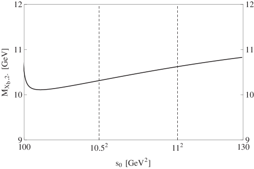
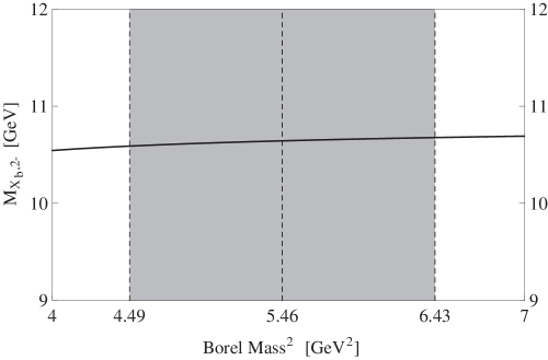
Figure 4: The variation of $M_{X}$ with respect to the threshold value $s_{0}$ (left) and the Borel mass $M_{B}$ (right), calculated using the current $J_{2-}(bs\bar{b}\bar{s})$ of $J^{P}=0^{+}$. In the left figure, the Borel mass $M_{B}$ is fixed to be $M^{2}_{B}=5.0$ GeV². In the right figure, the threshold value $s_{0}$ is fixed to be $s_{0}=11^{2}$ GeV², and the Borel window is $4.49$ GeV² $\leq M_{B}^{2}\leq 6.43$ GeV².

The possible decay channels of the $X(4500)$ and $X(4700)$ can be investigated by performing the Fierz and color rearrangements on the currents $J_{2\pm}$ and changing them to mesonic-mesonic structures Chen:2016qju ; Chen:2006hy ; Chen:2007xr :

$$J_{2\pm} \rightarrow \Bigg{(}\big{[}\bar{s}_{a}\gamma_{\mu_{1}}c_{b}\big{]}\big{[}\bar{c}_{a}\gamma_{\mu_{2}}D_{\mu_{3}}D_{\mu_{4}}s_{b}\pm\{a\leftrightarrow b\}\big{]}$$

$$\oplus\big{[}\bar{s}_{a}\gamma_{\mu_{1}}\gamma_{5}c_{b}\big{]}\big{[}\bar{c}_{a}\gamma_{\mu_{2}}\gamma_{5}D_{\mu_{3}}D_{\mu_{4}}s_{b}\pm\{a\leftrightarrow b\}\big{]}$$

$$\oplus\big{[}\bar{s}_{a}\sigma_{\mu_{1}\rho}c_{b}\big{]}\big{[}\bar{c}_{a}\sigma_{\mu_{2}\rho}D_{\mu_{3}}D_{\mu_{4}}s_{b}\pm\{a\leftrightarrow b\}\big{]}\Bigg{)}$$

$$\times\left(g^{\mu_{1}\mu_{3}}g^{\mu_{2}\mu_{4}}+g^{\mu_{1}\mu_{4}}g^{\mu_{2}\mu_{3}}-g^{\mu_{1}\mu_{2}}g^{\mu_{3}\mu_{4}}/2\right)\,.$$

Besides these structures, their similar/relevant $[\bar{s}s][\bar{c}c]$ structures are also possible. Accordingly, we obtain the possible decay channels of the $X(4500)$ and $X(4700)$ to be $S$-wave $D_{s}^{*+}D_{s}^{*-}$, $D_{s}^{*+}D_{s1}^{*-}(2860)$, $D_{s}^{*+}D_{s3}^{*-}(2860)$, $J/\psi\phi$, $J/\psi\phi_{3}(1850)$, $P$-wave $D_{s}^{*+}D_{s0}^{*-}$, $D_{s}^{*+}D_{s1}^{-}$, $D_{s}^{*+}D_{s2}^{*-}$, and $D$-wave $D_{s}^{*+}D_{s}^{*-}$ and $J/\psi\phi$, etc. The $X(4500)$ and $X(4700)$ were observed by LHCb in the $J/\psi\phi$ channel, which probably contain both $S$-wave and $D$-wave components. However, the overlap of the $S$-wave $J/\psi\phi$ channel (as well as the $S$-wave $D_{s}^{*+}D_{s}^{*-}$ channel) and the $J_{2\pm}$ (containing the $D$-wave antidiquark) is quite small, which makes the widths of the $X(4500)$ and $X(4700)$ not very large.

To examine these interpretations, we have also studied the bottom partners of the $X(4500)$ and $X(4700)$ by simply replacing charm quarks to be bottom quarks. We evaluate their masses using the bottom quark mass $m_{b}(m_{b})=4.20\pm 0.07$ GeV in the $\overline{\rm MS}$ scheme Chen:2010ze ; Agashe:2014kda . We show the mass obtained using $J_{2-}(bs\bar{b}\bar{s})$ in Fig. 4 as a function of the threshold values $s_{0}$ and the Borel mass $M_{B}$. There is a mass plateau around $s_{0}\sim 10^{2}$ GeV², but it depends on the bottom quark mass, which has large uncertainty Agashe:2014kda . We choose $s_{0}=11^{2}$ GeV² Chen:2010ze (there exist Borel windows when $s_{0}\geq 10.5^{2}$ GeV²), and the mass obtained is around 10.64 GeV. The mass obtained using $J_{2+}(bs\bar{b}\bar{s})$ is also around 10.64 GeV. We propose to search for them in the $\Upsilon\phi$ invariant mass distribution with the running of LHC at 13 TeV and forthcoming BelleII.

Besides the above dependence on the bottom quark mass, the extracted masses of the $X(4500)$ and $X(4700)$ in the present work also depend on the running strange and charm quark masses, which further depend on the energy scale. Therefore, our results still have some extra theoretical uncertainties not included in Eqs. (19) and (20), and more theoretical and experimental studies are necessary to understand their internal structures. Especially, the determination/confirmation of their spin-parity quantum numbers in experiments can be essential. We also note that the $X(4140)$, $X(4274)$, $X(4500)$ and $X(4700)$ can have many partner states. If their interpretations in this letter are correct, their dual partner states would be quite interesting, such as the $S$-wave scalar and the $D$-wave axial-vector tetraquark states with the quark content $cs\bar{c}\bar{s}$. Especially in the diquark-antidiquark configuration, the $S$-wave scalar $cs\bar{c}\bar{s}$ tetraquark state consisting of two “bad” diquarks is the dual partner state of both the $X(4140)$ (by replacing one “good” diquark by one “bad” diquark) and the $X(4500)$ (as its ground state), which may also exist.

To end this paper, we note that we can also use the $S/P/D$-waves diquarks and antidiquarks to construct many other states, and we plan to use QCD sum rules to systematically study them. Although QCD sum rule studies can not predict their existence, our studies can still be helpful to experimental searching of new exotic hadrons.

References

(1)
W. Chen and S. L. Zhu,
Phys. Rev. D 83, 034010 (2011).
(2)
K. A. Olive et al. [Particle Data Group Collaboration],
Review of Particle Physics,
Chin. Phys. C 38, 090001 (2014).
(3)
R. L. Jaffe,
Phys. Rept. 409, 1 (2005).
(4)
X. Liu,
Chin. Sci. Bull. 59, 3815 (2014).
(5)
H. X. Chen, W. Chen, X. Liu and S. L. Zhu,
Phys. Rept. 639, 1 (2016).
(6)
R. Aaij et al. [LHCb Collaboration],
Phys. Rev. Lett. 115, 072001 (2015).
(7)
R. Aaij et al. [LHCb Collaboration], arXiv:1606.07895 [hep-ex];
R. Aaij et al. [LHCb Collaboration], arXiv:1606.07898 [hep-ex];
Talk given by T. Skwarnicki, on behalf of the LHCb Collaboration at Meson2016, see http://meson.if.uj.edu.pl/indico/event/3/session/1/contribution/ 16/material/slides/0.pdf;
Talk given by T. Britton, on behalf of the LHCb Collaboration at APS April Meeting 2016, see https://absuploads.aps.org/presentation.cfm?pid=11733.
(8)
T. Aaltonen et al. [CDF Collaboration],
Phys. Rev. Lett. 102, 242002 (2009).
(9)
T. Aaltonen et al. [CDF Collaboration],
arXiv:1101.6058 [hep-ex].
(10)
X. Liu, Z. G. Luo, Y. R. Liu and S. L. Zhu,
Eur. Phys. J. C 61, 411 (2009).
(11)
X. Liu and S. L. Zhu,
Phys. Rev. D 80, 017502 (2009)
Erratum: [Phys. Rev. D 85, 019902 (2012)].
(12)
N. Mahajan,
Phys. Lett. B 679, 228 (2009).
(13)
T. Branz, T. Gutsche and V. E. Lyubovitskij,
Phys. Rev. D 80, 054019 (2009).
(14)
G. J. Ding,
Eur. Phys. J. C 64, 297 (2009).
(15)
X. Liu, Z. G. Luo and S. L. Zhu,
Phys. Lett. B 699, 341 (2011)
Erratum: [Phys. Lett. B 707, 577 (2012)].
(16)
Z. G. Wang,
Int. J. Mod. Phys. A 26, 4929 (2011).
(17)
S. I. Finazzo, M. Nielsen and X. Liu,
Phys. Lett. B 701, 101 (2011).
(18)
J. He and X. Liu,
Eur. Phys. J. C 72, 1986 (2012).
(19)
C. Hidalgo-Duque, J. Nieves and M. P. Valderrama,
Phys. Rev. D 87, 076006 (2013).
(20)
F. Stancu,
J. Phys. G 37, 075017 (2010).
(21)
S. Patel, M. Shah and P. C. Vinodkumar,
Eur. Phys. J. A 50, 131 (2014).
(22)
R. Molina and E. Oset,
Phys. Rev. D 80, 114013 (2009).
(23)
T. Branz, R. Molina and E. Oset,
Phys. Rev. D 83, 114015 (2011).
(24)
I. V. Danilkin and Y. A. Simonov,
Phys. Rev. D 81, 074027 (2010).
(25)
E. van Beveren and G. Rupp,
arXiv:0906.2278 [hep-ph].
(26)
R. M. Albuquerque, M. E. Bracco and M. Nielsen,
Phys. Lett. B 678, 186 (2009).
(27)
J. R. Zhang and M. Q. Huang,
J. Phys. G 37, 025005 (2010).
(28)
Z. G. Wang,
Eur. Phys. J. C 63, 115 (2009).
(29)
Z. G. Wang, Z. C. Liu and X. H. Zhang,
Eur. Phys. J. C 64, 373 (2009).
(30)
H. X. Chen, A. Hosaka and S. L. Zhu,
Phys. Lett. B 650, 369 (2007).
(31)
H. X. Chen, W. Chen, X. Liu, T. G. Steele and S. L. Zhu,
Phys. Rev. Lett. 115, 172001 (2015).
(32)
H. X. Chen, D. Zhou, W. Chen, X. Liu and S. L. Zhu,
Eur. Phys. J. C 76, 602 (2016).
(33)
H. X. Chen, A. Hosaka and S. L. Zhu,
Phys. Rev. D 74, 054001 (2006).
(34)
H. X. Chen, A. Hosaka and S. L. Zhu,
Phys. Rev. D 76, 094025 (2007).
(35)
L. Maiani, F. Piccinini, A. D. Polosa and V. Riquer,
Phys. Rev. D 71, 014028 (2005).
(36)
R. T. Kleiv, T. G. Steele, A. Zhang and I. Blokland,
Phys. Rev. D 87, 125018 (2013).
(37)
R. F. Lebed and A. D. Polosa,
Phys. Rev. D 93, 094024 (2016).
(38)
M. A. Shifman, A. I. Vainshtein and V. I. Zakharov,
Nucl. Phys. B 147, 385 (1979).
(39)
L. J. Reinders, H. Rubinstein and S. Yazaki,
Phys. Rept. 127, 1 (1985).
(40)
M. Nielsen, F. S. Navarra and S. H. Lee,
Phys. Rept. 497, 41 (2010).
(41)
P. Colangelo and A. Khodjamirian, “At the Frontier of
Particle Physics/Handbook of QCD” (World Scientific,
Singapore, 2001), Volume 3, 1495.