Finding Low-Rank Solutions via Non-Convex Matrix Factorization, Efficiently and Provably

Abstract

A rank-$r$ matrix $X\in\mathbb{R}^{m\times n}$ can be written as a product $UV^{\top}$, where $U\in\mathbb{R}^{m\times r}$ and $V\in\mathbb{R}^{n\times r}$. One could exploit this observation in optimization: e.g., consider the minimization of a convex function $f(X)$ over rank-$r$ matrices, where the set of rank-$r$ matrices is modeled via the factorization $UV^{\top}$. Though such parameterization reduces the number of variables, and is more computationally efficient (of particular interest is the case $r\ll\min\{m,n\}$), it comes at a cost: $f(UV^{\top})$ becomes a non-convex function w.r.t. $U$ and $V$.

We study such parameterization for optimization of generic convex objectives $f$, and focus on first-order, gradient descent algorithmic solutions. We propose the Bi-Factored Gradient Descent (BFGD) algorithm, an efficient first-order method that operates on the $U,V$ factors. We show that when $f$ is (restricted) smooth, BFGD has local sublinear convergence, and linear convergence when $f$ is both (restricted) smooth and (restricted) strongly convex. For several key applications, we provide simple and efficient initialization schemes that provide approximate solutions good enough for the above convergence results to hold.

1 Introduction

We study matrix problems of the form:

$$\underset{X\in\mathbb{R}^{m\times n}}{\text{minimize}} f(X),$$ (1)

where the minimizer $X^{\star}\in\mathbb{R}^{m\times n}$ is rank-$r^{\star}$ ($r^{\star}\leq\min\left\{m,n\right\}$), or approximately low rank, i.e., $\|X^{\star}-X^{\star}_{r^{\star}}\|_{F}$ is sufficiently small, for $X^{\star}_{r^{\star}}$ being the best rank-$r^{\star}$ approximation of $X^{\star}$. In our discussions, $f$ is a differentiable convex function; further assumptions on $f$ will be described later in the text. Note, in particular, that in the absence of further assumptions, $X^{\star}$ may not be unique.

Specific instances of (1), where the solution is assumed low-rank, appear in several applications in diverse research fields; a non-exhaustive list includes factorization-based recommender systems [89, 86, 38, 14, 63, 54], multi-label classification tasks [3, 15, 28, 78, 97, 101], dimensionality reduction techniques [88, 33, 60, 95, 49, 74], density matrix estimation of quantum systems [1, 48, 61], phase retrieval applications [26, 96], sensor localization [18, 99] and protein clustering [77] tasks, image processing problems [5], as well as applications in system theory [44], just to name a few. Thus, it is critical to devise user-friendly, efficient and provable algorithms that solve (1), taking into consideration such near low-rank structure of $X^{\star}$.

While, in general, imposing a low-rankness may result in an NP-hard problem, (1) with a rank-constraint can be solved in polynomial-time for numerous applications, where $f$ has specific structure. A prime—and by now well-known—example of this is the matrix sensing/matrix completion problem [24, 85, 54] (we discuss this further in Section 1.1). There, $f$ is a least-squares objective function and the measurements satisfy the appropriate restricted isometry/incoherence assumptions. In such a scenario, the optimal low-rank $X^{\star}$ can be recovered in polynomial time, by solving (1) with a rank-constraint [55, 13, 9, 70, 65, 91], or by solving its convex nuclear-norm relaxation, as in [72, 12, 22, 11, 32, 105].

In view of the above and although such algorithms have attractive convergence rates, they directly manipulate the $n\times n$ variable matrix $X$, which in itself is computationally expensive in the high-dimensional regime. Specifically, each iteration in these schemes typically requires computing the top-$r$ singular value/vectors of the matrix. As $n$ scales, these computational demands at each iteration can be prohibitive.

Optimizing over factors. In this paper, we follow a different path: a rank-$r$ matrix $X\in\mathbb{R}^{m\times n}$ can be written as a product of two matrices $UV^{\top}$, where $U\in\mathbb{R}^{m\times r}$ and $V\in\mathbb{R}^{n\times r}$. Based on this premise, we consider optimizing $f$ over the $U$ and $V$ space. Particularly, we are interested in solving (1) via the parametrization:

$$\underset{U\in\mathbb{R}^{m\times r},~{}V\in\mathbb{R}^{n\times r}}{\text{minimize}} f(UV^{\top})\quad\quad\quad\text{where $r\leq\mathrm{rank}(X^{\star})\leq\left\{m,~{}n\right\}$}.$$ (2)

Note that characterizations (2) and (1) are equivalent in the case $\text{rank}(X^{\star})=r$. Observe that such parameterization leads to a very specific kind of non-convexity in $f$. Even more importantly, proving convergence for these settings becomes a harder task, due to the bi-linearity of the variable space.

Motivation. Our motivation for studying (2) originates from large-scale problem instances: when $r$ is much smaller than $\min\{m,n\}$, factors $U\in\mathbb{R}^{m\times r}$ and $V\in\mathbb{R}^{n\times r}$ contain far fewer variables to maintain and optimize, than $X=UV^{\top}$. Thus, by construction, such parametrization also makes it easier to update and store the iterates $U,V$.

Even more importantly, observe that $UV^{\top}$ reformulation automatically encodes the rank constraint. Standard approaches, that operate in the original variable space, either enforce the $\mathrm{rank}(X)\leq r$ constraint at every iteration or involve a nuclear-norm projection. Doing so requires computing a truncated SVD per iteration, which can get cumbersome in large-scale settings. In stark contrast, working with $f(UV^{\top})$ replaces singular value computation per iteration with matrix-matrix multiplication operations. Thus, such non-conventional approach turns out to be a more practical and realistic option, when the dimension of the problem is large. We defer this discussion to Section 6.1 for some empirical evidence of the above.

Our contributions. While the computational gains are apparent, such bi-linear reformulations $X=UV^{\top}$often lack theoretical guarantees. Only recently, there have been attempts in providing answers to when and why such non-convex approaches perform well in practice, in the hope that they might provide a new algorithmic paradigm for designing faster and better algorithms; see [57, 4, 93, 107, 31, 16, 106, 90, 108, 59].

As we describe below and in greater detail in Section 1.2, our work is more general, addressing important settings that could not (as far as we know) be treated by the previous literature. Our contributions can be summarized as follows:

• We study a gradient descent algorithm on the non-convex formulation given in (2) for non-square matrices. We call this Bi-Factored Gradient Descent (BFGD). Recent developments (cited above, and see Section 1.2 for further details) rely on properties of $f$ for special cases [90, 93, 108, 106], and their convergence results seem to rely on this special structure. In this work, we take a more generic view of such factorization techniques, closer to results in convex optimization. We provide local convergence guarantees for general smooth (and strongly convex) $f$ objectives.

• In particular, when $f$ is only (restricted) smooth, we show that a simple lifting technique leads to a local sublinear rate convergence guarantee, using results from that of the square and PSD case [16]. Moreover, we provide a simpler and improved proof than [16], which requires a weaker initial condition.

• When $f$ is both (restricted) strongly convex and smooth, results from the PSD case do not readily extend. In such cases, of significant importance is the use of a regularizer in the objective, that restricts the geometry of the problem at hand. Here, we improve upon [93, 108, 104]—where such a regularizer was used only for the cases of matrix sensing/completion and robust PCA—and solve a different formulation that lead to local linear rate convergence guarantees. Our proof technique proves a significant generalization: using any smooth and strongly convex regularizer on the term $(U^{\top}U-V^{\top}V)$, with optimum at zero, one can guarantee linear convergence.

• Our theory is backed up with extensive experiments, including affine rank minimization (Section 6.3), compressed noisy image reconstruction from a subset of image pixels (Section 6.4), and 1-bit matrix completion tasks (Section 6.5). Overall, our proposed scheme shows superior recovery performance, as compared to state-of-the-art approaches, while being $(i)$ simple to implement, $(ii)$ scalable in practice and, $(iii)$ versatile to various applications.

1.1 When Such Optimization Criteria Appear in Practice?

In this section, we describe some applications that can be modeled as in (2). The list includes criteria with $(i)$ smooth and strongly convex objective $f$ (e.g., quantum state tomography from a limited set of observations and compressed image de-noising), and $(ii)$ just smooth objective $f$ (e.g., 1-bit matrix completion and logistic PCA). For all cases, we succinctly describe the problem and provide useful references on state-of-the-art approaches; we restrict our discussion on first-order, gradient schemes. Some discussion regarding recent developments on factorized approaches is deferred to Section 1.2. Section 6 provides specific configuration of our algorithm, for representative tasks, and make a comparison with state of the art.

1.1.1 Matrix Sensing Applications

Matrix sensing (MS) problems have gained a lot of attention the past two decades, mostly as an extension of Compressed Sensing [39, 10] to matrices; see [45, 85]. The task involves the reconstruction of an unknown and low-rank ground truth matrix $X^{\star}$, from a limited set of measurements. The assumption on low-rankness depends on the application at hand and often is natural: e.g., in background subtraction applications, $X^{\star}$ is a collection of video frames, stacked as columns, where the “action” from frame to frame is assumed negligible [25, 98]; in (robust) principal component analysis [29, 25], we intentionally search for a low-rank representation of the data; in linear system identification, the low rank $X^{\star}$ corresponds to a low-order linear, time-invariant system [76]; in sensor localization, $X^{\star}$ denotes the matrix of pairwise distances with rank-dependence on the, usually, low-dimensional space of the data [58]; in quantum state tomography, $X^{\star}$ denotes the density state matrix of the quantum system and $X^{\star}$ is designed to be rank-1 (pure state) or rank-$r$ (almost pure state), for $r$ relatively small [1, 46, 61].

In a non-factored form, MS is expressed via the following criterion:

$$\underset{X\in\mathbb{R}^{m\times n}}{\text{minimize}} f(X):=\tfrac{1}{2}\cdot\|y-\mathcal{A}(X)\|_{2}^{2}$$ (3)

subject to $$\text{rank}(X)\leq r,$$

where usually $m\neq n$ and $r\ll\min\{m,~{}n\}$. Here, $y=\mathcal{A}\left(X^{\star}\right)+\varepsilon\in\mathbb{R}^{p}$ contains the (possibly noisy) samples, where $p\ll m\cdot n$. Key role in recovering $X^{\star}$ plays the sampling operator $\mathcal{A}$: it can be a Gaussian-based linear map [45, 85], a Pauli-based measurement operator, used in quantum state tomography applications [75], a Fourier-based measurement operator, which leads to computational gains in practice due to their structure [64, 85], or even a permuted and sub-sampled noiselet linear operator, used in image and video compressive sensing applications [98].

Critical assumption for $\mathcal{A}$ that renders (3) a polynomially solvable problem, is the restricted isometry property (RIP) for low-rank matrices [23]:

Definition 1.1 (Restricted Isometry Property (RIP)).

A linear map $\mathcal{A}$ satisfies the $r$-RIP with constant $\delta_{r}$, if

$$(1-\delta_{r})\|X\|_{F}^{2}\leq\|\mathcal{A}(X)\|_{2}^{2}\leq(1+\delta_{r})\|X\|_{F}^{2},$$

is satisfied for all matrices $X\in\mathbb{R}^{n\times n}$ such that $\text{rank}(X)\leq r$.

It turns out linear maps that satisfy Definition 1.1 also satisfy the (restricted) smoothness and strong convexity assumptions [80]; see Theorem 2 in [30] and Section 2 for their definition.

State-of-the-art approaches. The most popularized approach to solve this problem is through convexification: [43, 85, 24] show that the nuclear norm $\|\cdot\|_{*}$ is the tightest convex relaxation of the non-convex $\text{rank}(\cdot)$ constraint and algorithms involving nuclear norm have been shown to be effective in recovering low-rank matrices. This leads to:

$$\underset{X\in\mathbb{R}^{n\times p}}{\text{minimize}} f(X) \|X\|_{*}\leq t,$$ subject to (4)

and its regularized variant:

$$\underset{X\in\mathbb{R}^{n\times p}}{\text{minimize}} f(X)+\lambda\cdot\|X\|_{*}.$$ (5)

Efficient implementations include Augmented Lagrange Multiplier (ALM) methods [72], convex conic solvers like the TFOCS software package [12] and, convex proximal and projected first-order methods [22, 11]. However, due to the nuclear norm, in most cases these methods are binded with full SVD computations per iteration, which constitutes them impractical in large-scale settings.

From a non-convex perspective, algorithms that solve (3) in a non-factored form include SVP and Randomized SVP algorithms [55, 13], Riemannian Trust Region Matrix Completion algorithm (RTRMC) [19], ADMiRA [70] and the Matrix ALPS framework [65, 91].

In all cases, algorithms admit fast linear convergence rates. Moreover, the majority of approaches assumes a first-order oracle: information of $f$ is provided through its gradient $\nabla f(X)$. For MS, $\nabla f(X)=-2\mathcal{A}^{*}\left(y-\mathcal{A}(X)\right)$, which requires $O({\rm T}_{\text{map}})$ complexity, where ${\rm T}_{\text{map}}$ denotes the time required to apply linear map (or its adjoint $\mathcal{A}^{*}$) $\mathcal{A}$. Formulations (3)-(5) require at least one top-$r$ SVD calculation per iteration; this translates into additional $O(mnr)$ complexity.

Motivation for factorizing (3). Problem (3) can be factorized as follows:

$$\underset{U\in\mathbb{R}^{n\times r},V\in\mathbb{R}^{p\times r}}{\text{minimize}} f(UV^{\top}):=\tfrac{1}{2}\cdot\|y-\mathcal{A}(UV^{\top})\|_{2}^{2}.$$ (6)

For this case and assuming a first-order oracle, the gradient of $f$ with respect to $U$ and $V$ can be computed respectively as $\nabla_{U}f(UV^{\top}):=\nabla f(X)V$ and $\nabla_{V}f(UV^{\top}):=\nabla f(X)^{\top}U$, respectively. This translates into $2\cdot O({\rm T}_{\text{map}}+mnr)$ time complexity. However, one avoids performing any SVD calculations per iteration, which in practice is considered a great computational bottleneck, even for moderate $r$ values. Thus, if there exist linearly convergent algorithms for (6), intuition indicates that one could obtain computational gains.

1.1.2 Logistic PCA and Low-Rank Estimation on Binary Data

Finding a low-rank approximation of binary matrices has gain a lot of interest recently, due to the wide appearance of categorical responses in real world applications [88, 33, 60, 95, 49, 74]. While regular linear principal component analysis (PCA) is still applicable for binary or categorical data, $(i)$ the way data are pre-processed (e.g., centering data before applying PCA), and/or $(ii)$ the least-squares objective in PCA, constitute it a natural choice for real-valued data, where observations are assumed to follow a Gaussian distribution. [92, 36] propose generalized versions of PCA for other type of data sets: In the case of binary data, this leads to Logistic Principal Component Analysis (Logistic PCA), where each binary data vector is assumed to follow the multivariate Bernoulli distribution, parametrized by the principal components that live in a $r$-dimensional subspace. Moreover, collaborative filtering on binary data and network sign prediction tasks have shown that standard least-squares loss functions perform poorly, while generic logistic loss optimization shows more interpretable and promising results.

To rigorously formulate the problem, let $Y\in\left\{0,1\right\}^{m\times n}$ be the observed binary matrix, where each of the $m$ rows stores a $n$-dimensional binary feature vector. Further, assume that each entry $Y_{ij}$ is drawn from a Bernoulli distribution with mean $q_{ij}$, according to: $\mathbb{P}\left[Y_{ij}~{}|~{}q_{ij}\right]=q_{ij}^{Y_{ij}}\cdot(1-q_{ij})^{1-Y_{ij}}$. Define the log-odds parameter $X_{ij}=\log\left(\tfrac{q_{ij}}{1-q_{ij}}\right)$ and the logistic function $\sigma(X_{ij})=\left(1+e^{-X_{ij}}\right)^{-1}$. Then, we equivalently have $\mathbb{P}\left[Y_{ij}~{}|~{}X_{ij}\right]=\sigma(X_{ij})^{Y_{ij}}\cdot\sigma(-X_{ij})^{1-Y_{ij}}$, or in matrix form,

$$\mathbb{P}\left[Y~{}|~{}X\right]=\prod_{ij}\sigma(X_{ij})^{Y_{ij}}\cdot\sigma(-X_{ij})^{1-Y_{ij}},$$

where we assume independence among entries of $Y$. The negative log-likelihood for log-odds parameter $X$ is given by:

$$f(X):=-\sum_{ij}\left(Y_{ij}\cdot\log\sigma(X_{ij})+\left(1-Y_{ij}\right)\cdot\log\sigma(-X_{ij})\right).$$

Assuming a compact, i.e., low-rank, representation for the latent variable $X$, we end up with the following optimization problem:

$$\underset{X\in\mathbb{R}^{m\times n}}{\text{minimize}} f(X):=-\sum_{ij}\left(Y_{ij}\cdot\log\sigma(X_{ij})+\left(1-Y_{ij}\right)\cdot\log\sigma(-X_{ij})\right)$$ (7)

subject to $$\text{rank}(X)\leq r;$$

observe that the objective criterion is just a smooth convex loss function.

State-of-the-art approaches. In [33], the authors consider the problem of sign prediction of edges in a signed network and cast it as a low-rank matrix completion problem: In order to model sign inconsistencies between the entries of binary matrices, the authors consider more appropriate loss functions to minimize, among which is the logistic loss. The proposed algorithmic solution follows (stochastic) gradient descent motions; however, no guarantees are provided. [60] utilizes logistic PCA for collaborative filtering on implicit feedback data (page clicks and views, purchases, etc.): to find a local minimum, an alternating gradient descent procedure is used—further, the authors use AdaGrad [42] to adaptively update the gradient descent step size, in order to reduce the number of iterations for convergence. A similar alternating gradient descent approach is followed in [88], with no known theoretical guarantees.

Motivation for factorizing (7). Following same arguments as before, in logistic PCA and logistic matrix factorization problems, we often assume that the observation binary matrix is generated as the sign operation on a linear factored model: $\texttt{sign}(UV^{T})$. Parameterized by the latent factors $U,V$, we obtain the following optimization criterion:

$$\underset{U\in\mathbb{R}^{m\times r},~{}V\in\mathbb{R}^{n\times r}}{\text{minimize}} f(UV^{\top}):=-\sum_{ij}\left(Y_{ij}\cdot\log\sigma(U_{i}V_{j}^{\top})+\left(1-Y_{ij}\right)\cdot\log\sigma(-U_{i}V_{j}^{\top})\right),$$ (8)

where $U_{i}$, $V_{j}$ represent the $i$-th and $j$-th row of $U$ and $V$, respectively.

1.2 Related Work

As it is apparent from the discussion above, this is not the first time such transformations have been considered in practice. Early works on principal component analysis [34, 87] and non-linear estimation procedures [102], use this technique as a heuristic; empirical evaluations show that such heuristics work well in practice [86, 50, 6]. [20, 21] further popularized these ideas for solving SDPs: their approach embeds the PSD and linear constraints into the objective and applies low-rank variable re-parameterization. While the constraint considered here is of different nature—i.e, rank constraint vs. PSD constraint—the motivation is similar: in SDPs, by representing the solution as a product of two factor matrices, one can remove the positive semi-definite constraint and thus, avoid computationally expensive projections onto the PSD cone.

We provide an overview of algorithms that solve instances of (2); for discussions on methods that operate on $X$ directly, we defer the reader to [2, 54, 65] for more details; see also Table 1 for an overview of the discussion below. We divide our discussion into two problem settings: $(i)$ $X^{\star}$ is square and PSD and, $(ii)$ $X^{\star}$ is non-square.

Algo.		$X$		$UU^{\top}$		$UV^{\top}$		Rate		Function $f$
[56]		✓		✗		✗		Linear		MS
[91]		✓		✗		✗		Linear		MS
[65]		✓		✗		✗		Linear		MS
[53]		✗		✓		✗		Sublinear		MS
[69]		✗		✓		✗		Sublinear		Convex $f$
[31]		✗		✓		✗		(Sub)linear		Generic $f^{\dagger}$
[16]		✗		✓		✗		(Sub)linear		Convex $f$
[54]		✗		✓		✓		Sublinear		Convex $f$
[93]		✗		✓		✓		Linear		MS
[107]		✗		✓		✓		Linear		MS
[52]		✗		✓		✓		Linear		MC
[56]		✗		✓		✓		Linear		MC, MS
[90]		✗		✓		✓		Linear		MC
[106]		✗		✓		✓		Linear		Strongly convex $f$
This work		✗		✓		✓		(Sub)linear		Convex $f$

Table 1: Summary of selected non-convex solvers for low-rank inference problems. $X$, $UU^{\top}$, and $UV^{\top}$ denote the setting the algorithm works at; $X$ means that no factorization is considered. “Rate” describes the convergence rate; “(Sub)linear” denotes that both sublinear and linear rates are proved, depending on the nature of $f$. “Function $f$” denotes the problems cases covered by each algorithm: “MS” and “MC” stand for matrix sensing and completion, respectively; “Convex $f$” corresponds to standard smooth and strongly convex functions $f$. For the case of [31], “Generic $f^{\dagger}$” corresponds to a specific class of functions that can be even concave but should satisfy specific conditions; see [31].

Square and PSD $X^{\star}$. A rank-$r$ matrix $X\in\mathbb{R}^{n\times n}$ is PSD if and only if it can be factored as $X=UU^{\top}$ for some $U\in\mathbb{R}^{n\times r}$. This is a special case of the problem discussed above, where $m=n$ and (1) includes a PSD constraint. Thus, after the re-parameterization, (2) takes the form:

$$\underset{U\in\mathbb{R}^{n\times r}}{\text{minimize}} f(UU^{\top})\quad\quad\quad\text{where $r=\text{rank}(X^{\star})\leq n$}.$$ (9)

Several recent works have studied (9). For the special case where $f$ is a least-squares objective for an underlying linear system, [93] and [107] propose gradient descent schemes that function on the factor $U$. Both studies employ careful initialization (performing few iterations of SVP [55] for the former and, using a spectral initialization procedure—as in [27]—for the latter) and step size selection, in order to prove convergence. However, their analysis is designed only for least-squares instances of $f$. Some results and discussion on their step size selection/initialization and how it compares with this work are provided in Section 6.

The work of [31] proposes a first-order algorithm for (9), where $f$ is more generic. The algorithmic solution proposed can handle additional constraints on the factors $U$; the nature of these constraints depends on the problem at hand. The authors present a broad set of exemplars for $f$—matrix completion and sensing, as well as sparse PCA, among others. For each problem, a set of assumptions need to be satisfied; i.e., faithfulness, local descent, local Lipschitz and local smoothness conditions; see [31] for more details. Under such assumptions and with proper initialization, one can prove convergence with $O(\nicefrac{{1}}{{\varepsilon}})$ or $O(\log(\nicefrac{{1}}{{\varepsilon}}))$ rate, depending on the nature of $f$, and for problems that even fail to be locally convex.

[16] proposes Factored Gradient Descent (FGD) algorithm for (9). FGD is also a first-order scheme; key ingredient for convergence is a novel step size selection that can be used for any $f$, as long as it is (restricted) gradient Lipschitz continuous; when $f$ is further (restricted) strongly convex, their analysis lead to faster convergence rates. Using proper initialization, this is the first paper that provably solves (9) for general convex functions $f$ and under common convex assumptions. An extension of these ideas to some constrained cases can be found in [82].

To summarize, most of these results guarantee convergence—up to linear rate—on the factored space, starting from a “good” initialization point and employing a carefully selected step size.

Non-square $X^{\star}$. [56] propose AltMinSense, an alternating minimization algorithm for matrix sensing and matrix completion problems. This is one of the first works to prove linear convergence in solving (2) for the MS model. [52] improves upon [56] for the case of reasonably well-conditioned matrices. Their algorithm handles problem cases with bad condition number and gaps in their spectrum [103]. Recently, [93] extended the Procrustes Flow algorithm to the non-square case, where gradient descent, instead of exact alternating minimization, is utilized. [108] extended the first-order method of [31] for matrix completion to the rectangular case. All the studies above focus on the case of least-squares objective $f$.

[90] generalize the results in [56, 52]: the authors show that, under common incoherence conditions and sampling assumptions, most first-order variants (e.g., gradient descent, alternating minimization schemes and stochastic gradient descent, among others) indeed converge to the low-rank ground truth $X^{\star}$. Both the theory and the algorithm proposed are restricted to the matrix completion objective.

Recently, [106]—based on the inexact first-order oracle, previously used in [8]—proved that linear convergence is guaranteed if $f(UV^{\top})$ is strongly convex over either $U$ and $V$, when the other is fixed. While the technique applies for generic $f$ and for non-square $X$, the authors provide algorithmic solutions only for matrix completion / matrix sensing settings. Furthermore, their algorithm requires QR-decompositions after each update of $U$ and $V$; this is required in order to control the notion of inexact first order oracle.

2 Preliminaries

Notation. For matrices $X,Y\in\mathbb{R}^{m\times n}$, $\left\langle X,Y\right\rangle=\operatorname{\textsc{Tr}}\left(X^{\top}Y\right)$ represents their inner product. We use $\left\|X\right\|_{F}$ and $\sigma_{1}(X)$ for the Frobenius and spectral norms of a matrix, respectively; we also use $\|X\|_{2}$ to denote spectral norm. Moreover, we denote as $\sigma_{i}(X)$ the $i$-th singular value of $X$. For a rank-$r$ matrix $X=UV^{\top}$, the gradient of $f$ w.r.t. $U$ and $V$ is $\nabla f(UV^{\top})V$ and $\nabla f(UV^{\top})^{\top}U$, respectively. With a slight abuse of notation, we will also use the terms $\nabla_{U}f(UV^{\top}):=\nabla f(UV^{\top})V$ and $\nabla_{V}f(UV^{\top}):=\nabla f(UV^{\top})^{\top}U$.

Given a matrix $X$, we denote its best rank-$r$ approximation with $X_{r}$; $X_{r}$ can be computed in polynomial time via the SVD. For our discussions from now on and in an attempt to simplify our notation, we denote the optimum point we search for as $X^{\star}_{r}$, both $(i)$ in the case where we intentionally restrict our search to obtain a rank-$r$ approximation of $X^{\star}$—while $\text{rank}(X^{\star})>r$—and $(i)$ in the case where $X^{\star}\equiv X^{\star}_{r}$, i.e., by default, the optimum point is of rank $r$.

An important issue in optimizing $f$ over the factored space is the existence of non-unique possible factorizations for a given $X$. Since we are interested in obtaining a low-rank solution in the original space, we need a notion of distance to the low-rank solution $X^{\star}_{r}$ over the factors. Among infinitely many possible decompositions of $X^{\star}_{r}$, we focus on the set of “equally-footed” factorizations [93]:

$$\mathcal{X}^{\star}_{r}=\Big{\{} \left(U^{\star},V^{\star}\right):~{}U^{\star}\in\mathbb{R}^{m\times r},V^{\star}\in\mathbb{R}^{n\times r},$$

$$\quad\quad\quad\quad\quad U^{\star}{V^{\star}}^{\top}=X^{\star}_{r},\sigma_{i}(U^{\star})=\sigma_{i}(V^{\star})=\sigma_{i}(X^{\star}_{r})^{1/2},\forall i\in[r]\Big{\}}.$$ (10)

Note that $(U^{\star},V^{\star})\in\mathcal{X}^{\star}_{r}$ if and only if the pair can be written as $U^{\star}=A^{\star}\Sigma^{\star 1/2}R,~{}V^{\star}=B^{\star}\Sigma^{\star 1/2}R$, where $A^{\star}\Sigma^{\star}B^{\star}$ is the singular value decomposition of $X^{\star}_{r}$, and $R\in\mathbb{R}^{r\times r}$ is an orthogonal matrix.

Given a pair $(U,V)$, we define the distance to $X^{\star}_{r}$ as:

$${\rm{\textsc{Dist}}}\left(U,V;X^{\star}_{r}\right)=\min_{(U^{\star},V^{\star})\in\mathcal{X}^{\star}_{r}}\left\|{\begin{bmatrix}U\\ V\end{bmatrix}-\begin{bmatrix}U^{\star}\\ V^{\star}\end{bmatrix}}\right\|_{F}.$$

Assumptions. We consider applications that can be described $(i)$ either by restricted strongly convex functions $f$ with gradient Lipschitz continuity, or $(ii)$ by convex functions $f$ that have only Lipschitz continuous gradients. We state these standard definitions below.

Definition 2.1.

Let $f:\mathbb{R}^{m\times n}\rightarrow\mathbb{R}$ be a convex differentiable function. Then, $f$ is gradient Lipschitz continuous with parameter $L$ (or $L$-smooth) if:

$$\left\|\nabla f\left(X\right)-\nabla f\left(Y\right)\right\|_{F}\leq L\cdot\left\|X-Y\right\|_{F},$$ (11)

$\forall X,Y\in\mathbb{R}^{m\times n}.$

Definition 2.2.

Let $f:\mathbb{R}^{m\times n}\rightarrow\mathbb{R}$ be convex and differentiable. Then, $f$ is $\mu$-strongly convex if:

$$f(Y)\geq f(X)+\left\langle\nabla f\left(X\right),Y-X\right\rangle+\tfrac{\mu}{2}\left\|Y-X\right\|_{F}^{2},$$ (12)

$\forall X,Y\in\mathcal{X}\subseteq\mathbb{R}^{m\times n}$.

The Factored Gradient Descent (FGD) algorithm. Part of our contributions is inspired by the work of [16], where the FGD algorithm is proposed. For completeness, we describe here the problem they consider and the proposed algorithm. [16] considers the problem:

$$\underset{X\in\mathbb{R}^{n\times n}}{\text{minimize}} f(X), X\succeq 0,$$ subject to

and proposes the following first-order recursion for its solution:

$$U_{t+1}=U_{t}-\eta\cdot\nabla f(U_{t}U_{t}^{\top})\cdot U_{t}.$$

Key property in their analysis is the positive semi-definiteness of the feasible space. For a proper initialization and step size, [16] show sublinear and linear convergence rates towards optimum, depending on the nature of $f$.

3 The Bi-Factored Gradient Descent (BFGD) Algorithm

In this section, we provide an overview of the Bi-Factored Gradient Descent (BFGD) algorithm for two problem settings in (1): $(i)$ $f$ being a $L$-smooth convex function and, $(ii)$ $f$ being $L$-smooth and $\mu$-strongly convex. For both cases, we assume a good initialization point $X_{0}=U_{0}V_{0}^{\top}$ is provided; for a discussion regarding initialization, see Section 5. Given $X_{0}$ and under proper assumptions, we further describe the theoretical guarantees that accompany BFGD.

As introduced in Section 1, BFGD is built upon non-convex gradient descent over each factor $U$ and $V$, written as

$$U_{t+1}=U_{t}-\eta\cdot\nabla_{U}f(U_{t}V_{t}^{\top}), \quad V_{t+1}=V_{t}-\eta\cdot\nabla_{V}f(U_{t}V_{t}^{\top}).$$ (13)

When $f$ is convex and smooth, BFGD follows exactly the motions in (13); in the case where $f$ is also strongly convex, BFGD is based on a different set of recursions, which we discuss in more detail in the rest of the section.

3.1 Reduction to FGD: When $f$ is Convex and $L$-Smooth

In [54], the authors describe a simple technique to transform problems similar to (1) into problems where we look for a square and PSD solution. The key idea is to lift the problem and introduce a stacked matrix of the two factors, as follows:

$$W=\begin{bmatrix}U\\ V\end{bmatrix}\in\mathbb{R}^{(m+n)\times r},$$

and optimize over a new function $\hat{f}:\mathbb{R}^{(m+n)\times(m+n)}\to\mathbb{R}$ defined as

$$\hat{f}\left(WW^{\top}\right)=\hat{f}\left(\begin{bmatrix}UU^{\top}&UV^{\top}\\ VU^{\top}&VV^{\top}\end{bmatrix}\right)=f(UV^{\top}).$$

Following this idea, one can utilize algorithmic solutions designed only to work on square and PSD-based instances of (1), where $f$ is just $L$-smooth. Here, we use the Factored Gradient Descent (FGD) algorithm of [16] on the $W$-space, as follows:

$$W_{t+1}=W_{t}-\eta\cdot\nabla_{W}\hat{f}(W_{t}W_{t}^{\top}).$$ (14)

Then, it is easy to verify the following remark:

Remark 1.

Define

$$\hat{f}\left(\begin{bmatrix}A&B\\ C&D\end{bmatrix}\right)=\frac{1}{2}f(B)+\frac{1}{2}f(C^{\top})$$

for $A\in\mathbb{R}^{m\times m}$, $B\in\mathbb{R}^{m\times n}$, $C\in\mathbb{R}^{n\times m}$, $D\in\mathbb{R}^{n\times n}$. Then FGD for minimizing $\hat{f}(WW^{\top})$ with the stacked matrix $W=[U^{\top},V^{\top}]^{\top}\in\mathbb{R}^{(m+n)\times r}$ is equivalent to (13).

A natural question is whether this reduction gives a desirable convergence behavior. Since FGD solves for a different function $\hat{f}$ from the original $f$, the convergence analysis depends also on $\hat{f}$. When $f$ is convex and smooth, we can rely on the result from [16].

Proposition 3.1.

If $f$ is convex and $L$-smooth, then $\hat{f}$ is convex and $\tfrac{L}{2}$-smooth.

Proof.

For any $Z_{1}=\begin{bmatrix}A_{1}&B_{1}\\ C_{1}&D_{1}\end{bmatrix},Z_{2}=\begin{bmatrix}A_{2}&B_{2}\\ C_{2}&D_{2}\end{bmatrix}\in\mathbb{R}^{(m+n)\times(m+n)}$, we have

$$\left\|\nabla\hat{f}(Z_{1})-\nabla\hat{f}(Z_{2})\right\|_{F} =\left\|\begin{bmatrix}0&\tfrac{1}{2}\cdot\nabla f(B_{1})\\ \tfrac{1}{2}\cdot\nabla f(C_{1}^{\top})^{\top}&0\end{bmatrix}-\begin{bmatrix}0&\tfrac{1}{2}\cdot\nabla f(B_{2})\\ \tfrac{1}{2}\cdot\nabla f(C_{2}^{\top})^{\top}&0\end{bmatrix}\right\|_{F}$$

$$=\tfrac{1}{2}\cdot\sqrt{\left\|\nabla f(B_{1})-\nabla f(B_{2})\right\|_{F}^{2}+\left\|\nabla f(C_{1}^{\top})-\nabla f(C_{2}^{\top})\right\|_{F}^{2}}$$

$$\leq\tfrac{L}{2}\cdot\sqrt{\left\|B_{1}-B_{2}\right\|_{F}^{2}+\left\|C_{1}-C_{2}\right\|_{F}^{2}}$$

$$\leq\tfrac{L}{2}\cdot\|Z_{1}-Z_{2}\|_{F}$$

where the first inequality follows from the $L$-smoothness of $f$. ∎

Based on the above proposition, we use FGD to solve (2) with $\hat{f}$: its procedure is exactly (13), with a different step size:

$$\eta \leq\frac{1}{20L\left\|{\begin{bmatrix}U_{0}\\ V_{0}\end{bmatrix}}\right\|_{2}^{2}+3\|\nabla f(U_{0}V_{0}^{\top})\|_{2}}.$$ (15)

While one can rely on the sublinear convergence analysis from [16], we provide a new guarantee with a weaker initial condition; see Section 4.

3.2 Using BFGD when $f$ is $L$-Smooth and Strongly Convex

Assume $f$ function satisfies both properties in Definitions 2.1 and 2.2. In this case, we cannot simply rely on the lifting technique as above since $\hat{f}$ is clearly not strongly convex. Instead, we consider a slight variation, where we appropriately regularize the objective and force the solution pair $(\widehat{U},\widehat{V})$ to be “balanced”. This regularization is based on the set of optimal pairs $(U^{\star},V^{\star})$ in $\mathcal{X}^{\star}_{r}$, as defined in (10). In particular, given $\mathcal{X}^{\star}_{r}$, the equivalent optimization problem that “forces” convergence to balanced $(U^{\star},V^{\star})$ is as follows:

$$\underset{U\in\mathbb{R}^{m\times r},~{}V\in\mathbb{R}^{n\times r}}{\text{minimize}} f(UV^{\top})+\lambda\cdot g(U^{\top}U-V^{\top}V),$$ (16)

where $g:\mathbb{R}^{r\times r}\to\mathbb{R}$ is an additional convex regularizer. We require:

• $g$ is convex and minimized at zero point; i.e., $\nabla g(0)=0$.

• The gradient, $\nabla g(U^{\top}U-V^{\top}V)\in\mathbb{R}^{r\times r}$ , is symmetric for any such pair.

• $g$ is $\mu_{g}$-strongly convex and $L_{g}$-smooth.

Under such assumptions, the addition of $g$ in the objective just restricts the set of optimum points to be “balanced”, i.e., the minimizer of (16) minimizes also (2).

The necessity of the regularizer. As we show next, the theoretical guarantees of BFGD heavily depend on the condition number of the pair $(U^{\star},V^{\star})$ the algorithm converges to. In particular, one of the requirements of BFGD is that every estimate $U_{t}$ (resp. $V_{t}$) be “relatively close” to the convergent point $U^{\star}$ (resp. $V^{\star}$), such that their distance $\|U_{t}-U^{\star}\|_{F}$ is bounded by a function of $\sigma_{r}(U^{\star})$, for all $t$. Then, it is easy to observe that, for arbitrarily ill-conditioned $(U^{\star},V^{\star})\in\mathcal{X}_{r}^{*}$, such a condition might not be easily satisfied by BFGD per iteration, unless we “force” the sequence of estimates $(U_{t},V_{t}),~{}\forall t,$ to converge to a better conditioned pair $(U^{\star},V^{\star})$. This is the key role of regularizer $g$: it guarantees putative estimates $U_{t}$ and $V_{t}$ are not too ill-conditioned, per iteration.

An example of $g$ is the Frobenius norm (weighted by $\mu/2$), as proposed in [93]. Other examples are sums of element-wise (at least) $\mu_{g}$-strongly convex and (at most) $L_{g}$-gradient Lipschitz functions (of the form $g(X)=\sum_{i,j}g_{ij}(X_{ij})$) with the optimum at zero. However, any other user-friendly $g$ can be selected, as long as it satisfies the above conditions. We show in this paper that any such regularizer results provably in convergence, with attractive convergence rate; see Section 6.2 for a toy example where the addition of $g$ leads to faster convergence rate in practice.

The BFGD algorithm. BFGD is a first-order, gradient descent algorithm for (16), that operates on the factored space $(U,V)$ in an alternating fashion. Principal components of BFGD is a proper step size selection and a “decent” initialization point. BFGD can be considered as the non-squared extension of FGD algorithm in [16], which is specifically designed to solve problems as in (2), for $U=V$ and $m=n$. The key differences with FGD though, other than the necessity of a regularizer $g$, are:

• Our analysis leads to provable convergence results in the non-square case. Such a result cannot be trivially obtained from [16].

• The main recursion followed is different in the two schemes: in the non-squared case, we update the left and right factors $(U,~{}V)$ with a different rule, according to which:

  $$U_{t+1} =U_{t}-\eta\left(\nabla_{U}f(U_{t}V_{t}^{\top})+\lambda\cdot\nabla_{U}g(U_{t}^{\top}U_{t}-V_{t}^{\top}V_{t})\right),$$

  $$V_{t+1} =V_{t}-\eta\left(\nabla_{V}f(U_{t}V_{t}^{\top})+\lambda\cdot\nabla_{V}g(U_{t}^{\top}U_{t}-V_{t}^{\top}V_{t})\right).$$

  The parameter $\lambda>0$ is arbitrarily chosen.

• Due to this new update rule, a slightly different and proper step size selection should be devised for BFGD. Our step size is selected as follows:

  $${}\eta\leq\frac{1}{12\cdot\max\left\{L,~{}L_{g}\right\}\cdot\left\|{\begin{bmatrix}U_{0}\\ V_{0}\end{bmatrix}}\right\|_{2}^{2}}.$$ (17)

  Compared to the step size proposed in [16] (which is of the same form with (15)), our analysis drops the dependence to $\|\nabla f(\cdot)\|_{2}$ at the denominator. This is leads to a faster computed step size and highlights the non-necessity of this term for proof of convergence, i.e., the presence of the $\|\nabla f(\cdot)\|_{2}$ term is sufficient but not necessary.

Algorithm 1 BFGD for smooth and strongly convex $f$

1:  Input: Function $f$, target rank $r$, # iterations $T$.

2:  Set initial values for $U_{0},V_{0}$

3:  Set step size $\eta$ as in (17).

4:  for $t=0$ to $T-1$ do

5:     $U_{t+1}=U_{t}-\eta\left(\nabla_{U}f(U_{t}V_{t}^{\top})-\lambda\cdot\nabla_{U}g(U_{t}^{\top}U_{t}-V_{t}^{\top}V_{t})\right)$

6:     $V_{t+1}=V_{t}-\eta\left(\nabla_{V}f(U_{t}V_{t}^{\top})-\lambda\cdot\nabla_{V}g(U_{t}^{\top}U_{t}-V_{t}^{\top}V_{t})\right)$

7:  end for

8:  Output: $X=U_{T}V_{T}^{\top}$.

The scheme is described in Algorithm 1. As shown in the next section, constant step size (17) is sufficient to lead to attractive convergence rates for BFGD, for $f$ $L$-smooth and $\mu$-strongly convex.

4 Local Convergence for BFGD

This section includes the main theoretical guarantees of BFGD, both for the cases of just smooth $f$, and $f$ being smooth and strongly convex. To provide such local convergence results, we assume that there is a known “good” initialization which ensures the following.

Assumption A1. Define $\kappa=\tfrac{\max\{L,L_{g}\}}{\min\{\mu,\mu_{g}\}}$ where $\mu_{g}$ and $L_{g}$ are the strong convexity and smoothness parameters of $g$, respectively. Then, we assume we are provided with a “good” initialization point $X_{0}=U_{0}V_{0}^{\top}$ such that:

$${\rm{\textsc{Dist}}}(U_{0},V_{0};X^{\star}_{r}) \leq\tfrac{\sqrt{2}\cdot\sigma_{r}(X^{\star}_{r})^{1/2}}{10\sqrt{\kappa}}\quad\quad\quad\quad\quad\text{(Strongly convex and smooth }f\text{)}.$$

$$\text{{For the case where }}f$$ is just smooth, we assume:

$${\rm{\textsc{Dist}}}(U_{0},V_{0};X^{\star}_{r}) \leq\tfrac{\sqrt{2}\cdot\sigma_{r}(X^{\star}_{r})^{1/2}}{10}\quad\quad\quad\quad\quad\text{(Smooth $f$)}.$$

For our analysis, we will use the following step size assumptions:

$$\widehat{\eta} \leq\frac{1}{8\max\{L,L_{g}\}\cdot\left\|{\begin{bmatrix}U_{t}\\ V_{t}\end{bmatrix}}\right\|_{2}^{2}}~{}\quad\quad\quad\quad\quad\quad\text{(Strongly convex and smooth }f\text{)},$$ (18)

$$\widehat{\eta} \leq\frac{1}{15L\left\|{\begin{bmatrix}U_{t}\\ V_{t}\end{bmatrix}}\right\|_{2}^{2}+3\|\nabla f(U_{t}V_{t}^{\top})\|_{2}}~{}\quad\quad\quad\text{(Smooth $f$)}.$$ (19)

While these step sizes are different than the ones we use in practice, there is a constant-fraction connection between $\widehat{\eta}$ and $\eta$.

Lemma 4.1.

Let $(U_{0},V_{0})$ be such that Assumption A1 is satisfied. Then, (18) holds if (17) is satisfied, and (19) holds if (15) is satisfied.

The proof is provided in the Appendix A. By this lemma, our analysis below is equivalent—up to constants—to that if we were using the original step size $\eta$ of the algorithm. However, for clarity reasons and ease of exposition, we use $\widehat{\eta}$ below.

For the case of strongly convex $f$, both Assumption A1 and the step size depends on the strong convexity and smoothness parameters of $g$. When $\mu$ and $L$ are known a priori, this dependency can be removed since one can choose $g$ such that at least $\mu$-restricted strongly convex and at most $L$-smooth. Then, $\kappa$ becomes the condition number of $f$, and the step size depends only on $L$.

4.1 Linear Local Convergence Rate when $f$ is $L$-Smooth and $\mu$-Strongly Convex

The following theorem proves that, under proper initialization, BFGD admits linear convergence rate, when $f$ is both $L$-smooth and $\mu$-restricted strongly convex.

Theorem 4.2.

Suppose that $f$ is $L$-smooth and $\mu$-restricted strongly convex and regularizer $g$ is $L_{g}$-smooth and $\mu_{g}$-restricted strongly convex. Define $\mu_{\min}:=\min\left\{\mu,\mu_{g}\right\}$ and $L_{\max}:=\max\left\{L,L_{g}\right\}$. Denote the unique minimizer of $f$ as $X^{\star}\in\mathbb{R}^{m\times n}$ and assume that $X^{\star}$ is of arbitrary rank. Let $\widehat{\eta}$ be defined as in (18). If the initial point $(U_{0},V_{0})$ satisfies Assumption A1, then BFGD algorithm in Algorithm 1 converges linearly to $X^{\star}_{r}$, within error $O\left(\sqrt{\frac{\kappa}{\sigma_{r}(X^{\star}_{r})}}\left\|{X^{\star}-X^{\star}_{r}}\right\|_{F}\right)$, according to the following recursion:

$${\rm{\textsc{Dist}}}(U_{t+1},V_{t+1};X^{\star}_{r})^{2}\leq\gamma_{t}\cdot{\rm{\textsc{Dist}}}(U_{t},V_{t};X^{\star}_{r})^{2}+\widehat{\eta}L\left\|{X^{\star}-X^{\star}_{r}}\right\|_{F}^{2},$$ (20)

for every $t\geq 0$, where the contraction parameter $\gamma_{t}$ satisfies:

$$\gamma_{t}=1-\widehat{\eta}\cdot\tfrac{\mu_{\min}\cdot\sigma_{r}(X^{\star}_{r})}{8} \geq 1-\tfrac{\mu_{\min}}{17\cdot L_{\max}}\cdot\tfrac{\sigma_{r}(X^{\star}_{r})}{\sigma_{1}(X^{\star}_{r})}>0.$$

The proof is provided in Section B. The theorem states that if $X^{\star}$ is (approximately) low-rank, the iterates converge to a close neighborhood of $X^{\star}_{r}$.

The above result can also be expressed w.r.t. the function value $f(UV^{\top})$, as follows:

Corollary 4.3.

Under the same initial condition with Theorem 4.2, Algorithm (1) satisfies the following recursion w.r.t. the distance of function values from the optimal point:

$$f(U_{t}V_{t}^{\top})-f(X^{\star})\leq\gamma^{t}\cdot\sigma_{1}(X^{\star})\cdot\left(f(U_{0}V_{0}^{\top})-f(X^{\star})\right)+\frac{\sqrt{\mu L}}{\sigma_{r}(X^{\star})}\left\|{X^{\star}-X^{\star}_{r}}\right\|_{F}^{2}.$$

4.2 Local Sublinear Convergence

In Section 3.1, we showed that a lifting technique can reduce our problem (2) to a rank-constrained semidefinite program, and applying FGD from [16] is exactly BFGD (13). While the sublinear convergence guarantee of FGD can also be applied to our problem, we provide an improved result.

Theorem 4.4.

Suppose that $f$ is $L$-smooth with a minimizer $X^{\star}\in\mathbb{R}^{m\times n}$. Let $\hat{X}_{r}$ be any target rank-$r$ matrix, and let $\widehat{\eta}$ be defined as in (19). If the initial point $X_{0}=U_{0}V_{0}^{\top}$, $U_{0}\in\mathbb{R}^{m\times r}$ and $V_{0}\in\mathbb{R}^{n\times r}$, satisfies Assumption A1, then FGD converges with rate $O(1/T)$ to a tolerance value according to:

$$f(U_{T}V_{T}^{\top})-f(U^{\star}{V^{\star}}^{\top})=\hat{f}(W_{T}W_{T}^{\top})-\hat{f}(W^{\star}{W^{\star}}^{\top})\leq\frac{10\cdot{\rm{\textsc{Dist}}}(U_{0},V_{0};X^{\star}_{r})^{2}}{\eta T}$$

Theorem 4.4 guarantees a local sublinear convergence with a looser initial condition. While [16] requires $\min_{R\in O(r)}\left\|{W-W^{\star}R}\right\|_{F}\leq\frac{\sigma_{r}^{2}(W^{\star})}{100\sigma_{1}^{2}(W^{\star})}\cdot\sigma_{r}(W^{\star})$, our result requires that the initial distance to the $W^{\star}$ is merely a constant factor of $\sigma_{r}(W^{\star})$.

5 Initialization

In this section, we present initialization procedures for the case where $f$ is strongly convex and smooth. Our main theorem guarantees linear convergence in the factored space given that the initial point $(U_{0},V_{0})$ is within a ball around the closest target factors, with radius $O(\kappa^{-1/2}\sigma_{r}(X^{\star}_{r})^{1/2})$. To find such a solution, we propose an extension of the initialization in [16].

Lemma 5.1.

Consider an initial solution $U_{0}V_{0}^{\top}$ which is the best rank-$r$ approximation of

$$X_{0}=-\tfrac{1}{L}\nabla f(0)$$ (21)

Then we have

$$\left\|{U_{0}V_{0}^{\top}-X^{\star}_{r}}\right\|_{F} \leq 2\sqrt{2\left(1-\tfrac{1}{\kappa}\right)}\left\|{X^{\star}}\right\|_{F}+2\left\|{X^{\star}-X^{\star}_{r}}\right\|_{F}$$

Combined with Lemma 5.14 in [93], which transforms a good initial solution from the original space to the factored space, the following corollary gives one sufficient condition for global convergence of BFGD with the SVD of (21) as initialization.

Corollary 5.2.

If

$$\left\|{X^{\star}-X^{\star}_{r}}\right\|_{F}\leq\frac{\sigma_{r}(X^{\star})}{100\sqrt{\kappa}},\quad\kappa\leq 1+\frac{\sigma_{r}(X^{\star}_{r})^{2}}{4608\cdot\left\|{X^{\star}_{r}}\right\|_{F}^{2}}$$

then the initial solution

$$U_{0}=A_{0}\Sigma_{0}^{1/2},~{}V_{0}=B_{0}\Sigma_{0}^{1/2}$$

where $A_{0}\Sigma_{0}B_{0}$ is the SVD of $-\frac{1}{L}\nabla f(0)$ satisfies the initial condition of Theorem 4.2.

Corollary 5.2 requires weaker conditions than [16] in order Theorem 4.2 be transformed to global guarantees. While our theoretical results can only guarantee global convergence for a well-conditioned problem ($\kappa$ close to one), we show in the experiments that the algorithm performs well in practice where the sufficient conditions are yet to be satisfied.

6 Experiments

In this section, we first provide comparison results regarding the actual computational complexity of SVD and matrix-matrix multiplication procedures; while such comparison is not thoroughly complete, it provides some evidence about the gains of optimizing over $U,V$ factors, in lieu of SVD-based rank-$r$ approximations. We also describe a toy example that highlights the effect of the regularizer $g$ in convergence rates, for strongly convex and smooth $f$. Next, we provide extensive results on the performance of BFGD, as compared with state of the art, for the following problem settings: $(i)$ affine rank minimization, where the objective is smooth and (restricted) strongly convex, $(ii)$ image denoising/recovery from a limited set of observed pixels, where the problem can be cast as a matrix completion problem, and $(iii)$ 1-bit matrix completion, where the objective is just smooth convex. In all cases, the task is to recover a low rank matrix from a set of observations, where our machinery naturally applies.

6.1 The Complexity of SVD and Matrix-Matrix Multiplication in Practice

To provide an idea of how matrix-matrix multiplication scales, in comparison with truncated SVD, we compare it with some state-of-the-art SVD subroutines: $(i)$ the Matlab’s svds subroutine, based on ARPACK software package [71], $(ii)$ a collection of implicitly-restarted Lanczos methods for fast truncated SVD and symmetric eigenvalue decompositions (irlba, irlbablk, irblsvds) [7] , $(iii)$ the limited memory block Krylov subspace optimization for computing dominant SVDs (LMSVD) [73], and $(iv)$ the PROPACK software package [68]. We consider random realizations of matrices in $\mathbb{R}^{m\times n}$ (w.l.o.g., assume $m=n$), for varying values of $m$. For SVD computations, we look for the best rank-$r$ approximation, for varying values of $r$. In the case of matrix-matrix multiplication, we record the time required for the computation of 2 matrix-matrix multiplications of matrices $\mathbb{R}^{m\times m}$ and $\mathbb{R}^{m\times r}$, which is equivalent with the computational complexity required in our scheme, in order to avoid SVD calculations. All experiments are performed in a Matlab environment.

Figure 1 (left panel) shows execution time results for the algorithms under comparison, as a function of the dimension $m$. Rank $r$ is fixed to $r=100$. While both SVD and matrix multiplication procedures are known to have $O(m^{2}r)$ complexity, it is obvious that the latter on dense matrices is at least two-orders of magnitude faster than the former. In Table 2, we also report the approximation guarantees of some faster SVD subroutines, as compared to svds: while irblablk seems to be faster, it returns a very rough approximation of the singular values, when $r$ is relatively large. Similar findings are depicted in Figures 1 (middle and right panel).

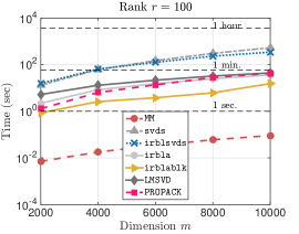
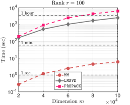
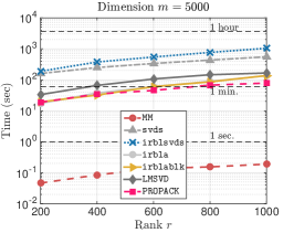
Figure 1: Comparison of SVD procedures versus Matrix Matrix (MM) multiplication. Left panel: Varying dimension $m$ and constant rank $r=100$. Middle panel: Similar to left panel where $m$ scales larger and we focus on a subset of SVD algorithms that can scale up. Right panel: Varying rank values and constant dimension $m=5\cdot 10^{3}$.

Algorithms		Error $\tfrac{\|\widehat{\Sigma}-\Sigma^{\star}\|_{F}}{\|\Sigma^{\star}\|_{F}}$, where $\Sigma^{\star}$ is diagonal matrix with top $r$ singular values from svds.
$\widehat{\Sigma}$		$m=2\cdot 10^{3}$		$m=4\cdot 10^{3}$		$m=6\cdot 10^{3}$		$m=8\cdot 10^{3}$		$m=10^{4}$
irblsvds		3.63e-15		4.33e-09		8.11e-11		4.79e-12		5.82e-10
irbla		6.00e-15		9.01e-07		1.05e-04		2.99e-04		7.29e-04
irblablk		1.48e+03		1.67e+03		1.24e+03		1.45e+03		7.91e+11
LMSVD		2.14e-14		4.49e-12		3.94e-11		1.33e-10		7.30e-10
PROPACK		4.10e-12		2.46e-10		1.63e-12		7.90e-12		3.55e-11

Table 2: Approximation errors of singular values, in the form $\tfrac{\|\widehat{\Sigma}-\Sigma^{\star}\|_{F}}{\|\Sigma^{\star}\|_{F}}$. Here, $\widehat{\Sigma}$ denote the diagonal matrix, returned by SVD subroutines, containing $r$ top singular values; we use svds to compute the reference matrix $\Sigma^{\star}$, that contains top-$r$ singular values of the input matrix. Observe that some algorithms deviate singificantly from the “ground-truth”: this is due to either early stopping (only a subset of singular values could be computed) or due to accumulating approximation error.

6.2 The Role of Regularizer $g$

In this section, we provide a simple example that illustrates the role of the regularizer $g$. As discussed in Section 3.2, $g$ forces our algorithm to converge to a well-conditioned factorization of $X^{\star}$. This regularizer not only enables us to control and guarantee convergence of BFGD, but also provides a better convergence rate, as we know next.

Figure 2 (left panel) shows the convergence behavior of BFGD, when $f$ and $f+g$ is used, with an ill-conditioned initial point $(U_{0},V_{0})$. It is obvious from the convergence plot that adding the regularizer results into faster convergence to an optimum. This difference in convergence rate is due to dependency on the condition numbers of $U^{\star}$ and $V^{\star}$ that the algorithm converges to. As shown in Figure 2 (right panel), the algorithm converges to a well-conditioned factorization of $X^{\star}$, while the condition number is not forced to decrease when there is no regularizer.

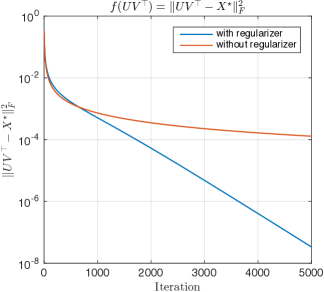
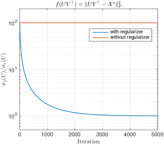
Figure 2: $f(UV^{\top})=\left\|{UV^{\top}-X^{\star}}\right\|_{F}^{2}$, where $X^{\star}=U^{\star}{V^{\star}}^{\top}\in\mathbb{R}^{100\times 100}$, and $U^{\star},V^{\star}\in\mathbb{R}^{100\times 10}$ are orthonormal. The initial point is an ill-conditioned (in particular $\sigma_{1}(U_{0})/\sigma_{r}(U_{0})=\sigma_{1}(V_{0})/\sigma_{r}(V_{0})=10^{2}$) pair of $X_{0}$ near $X^{\star}$. Left panel: Convergence behaviors of BFGD with a regularizer $g=\tfrac{1}{4}\left\|{U^{\top}U-V^{\top}V}\right\|_{F}^{2}$ and without any regularizer. Right panel: The ratios $\sigma_{1}(U)/\sigma_{r}(U)$ over iterations.

6.3 Affine Rank Minimization Using Noiselet Linear Maps

In this task, we consider the problem of affine rank minimization. In particular, we observe unknown $X^{\star}$ through a limited set of observations $y\in\mathbb{R}^{p}$, that satisfy:

$$y=\mathcal{A}\left(X^{\star}\right),$$ (22)

where $X^{\star}\in\mathbb{R}^{m\times n},~{}p\ll m\cdot n$, and $\mathcal{A}:\mathbb{R}^{m\times n}\rightarrow\mathbb{R}^{p}$ is a given linear map. The task is to recover $X^{\star}$, using $\mathcal{A}$ and $y$. Here, we use permuted and sub-sampled noiselets for the linear operator $\mathcal{A}$, due to their efficient implementation [98]; similar results can be obtained for $\mathcal{A}$ being a subsampled Fourier linear operator or, even, a random Gaussian linear operator. For the purposes of this experiment, the ground truth $X^{\star}$ is synthetically generated as the multiplication of two tall matrices, $U^{\star}\in\mathbb{R}^{m\times r}$ and $V^{\star}\in\mathbb{R}^{n\times r}$, such that $X^{\star}=U^{\star}V^{\star\top}$ and $\|X^{\star}\|_{F}=1$. Both $U^{\star}$ and $V^{\star}$ contain random, independent and identically distributed (i.i.d.) Gaussian entries, with zero mean and unit variance.

List of algorithms. We compare the following state-of-the-art algorithms: $(i)$ the Singular Value Projection (SVP) algorithm [55], a non-convex, projected gradient descent algorithm for (3), with constant step size selection (we study the case where $\mu=\nicefrac{{1}}{{3}}$, as it is the one that showed the best performance in our experiments), $(ii)$ the SparseApproxSDP extension to non-square cases for (5) in [54], based on [53], where a putative solution is refined via rank-1 updates from the gradient, $(iii)$ the matrix completion algorithm in [90], which we call GuaranteedMC, where the objective is (6), $(iv)$ the Procrustes Flow algorithm in [93] for (6), and $(v)$ the BFGD algorithm.

Implementation details. To properly compare the algorithms in the above list, we preset a set of parameters that are common. In all experiments, we fix the number of observations in $y$ to $p=C\cdot n\cdot r$, where $n\geq m$ in our cases, and for varying values of $C$. All algorithms in comparison are implemented in a Matlab environment, where no mex-ified parts present, apart from those used in SVD calculations; see below.

In all algorithms, we fix the maximum number of iterations to $T=4000$, unless otherwise stated. We use the same stopping criteria for the majority of algorithms as:

$$\frac{\|X_{t}-X_{t-1}\|_{F}}{\|X_{t}\|_{F}}\leq\rm{tol},$$ (23)

where $X_{t},~{}X_{t-1}$ denote the current and the previous estimates in the $X$ space and $\rm{tol}:=5\cdot 10^{-6}$. For SVD calculations, we use the lansvd implementation in PROPACK package [68]. For fairness, we modified all the algorithms so that they exploit the true rank $r$; however, we observed that small deviations from the true rank result in relatively small degradation in terms of the reconstruction performance.

In the implementation of BFGD, we set $g$ to be $\tfrac{1}{16}\cdot\|U^{\top}U-V^{\top}V\|_{F}^{2}$, as suggested in [93], for ease of comparison. Moreover, for our implementation of Procrustes Flow, we set the constant step size as $\mu:=\tfrac{2}{187}\cdot\{\tfrac{1}{\|U_{0}\|_{F}^{2}},\tfrac{1}{\|V_{0}\|_{F}^{2}\|}\}$, as suggested in [93]. We use the implementation of [90], with random initialization (unless otherwise stated) and regularization type soft, as suggested by their implementation. In [54], we require an upper bound on the nuclear norm of $X^{\star}$; in our experiments we assume we know $\|X^{\star}\|_{*}$, which requires a full SVD calculation. Moreover, for our experiments, we set the curvature constant for the SparseApproxSDP implementation to its true value $C_{f}=1$.

For initialization, we consider the following settings: $(i)$ random initialization, where $X_{0}=U_{0}V_{0}^{\top}$ for some randomly selected $U_{0}$ and $V_{0}$ such that $\|X_{0}\|_{F}=1$, and $(ii)$ specific initialization, as suggested in each of the papers above. Our specific initialization is based on the discussion in Section 5, where $X_{0}=\mathcal{P}_{r}(-\frac{1}{L}\nabla f(0))$. Algorithms SVP, SparseApproxSDP and the solver in [90] work with random initialization. For the initialization phase of [93], we consider two cases: $(i)$ the condition number $\kappa$ is known, where according to Theorem 3.3 in [93], we require $T_{\text{init}}:=\lceil 3\log(\sqrt{r}\cdot\kappa)+5\rceil$ SVP iterations, and $(ii)$ the condition number $\kappa$ is unknown, where we use Lemma 3.4 in [93].

Results using random initialization. Figure 3 depicts the convergence performance of the above algorithms w.r.t. total execution time. Top row corresponds to the case $m=n=1024$, bottom row to the case $m=2048,~{}n=4096$. For all cases, we fix $r=50$; from left to right, we decrease the number of available measurements, by decreasing the constant $C$. BFGD shows the best performance, compared to the rest of the algorithms. It is notable that BFGD performs better than SVP, by avoiding SVD calculations and employing a better step size selection. For this setting, GuaranteedMC converges to a local minimum while SparseApproxSDP and Procrustes Flow show close to sublinear convergence rate.

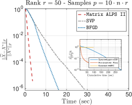
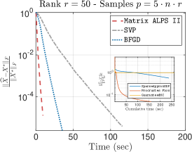
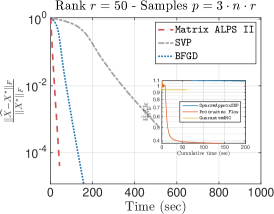
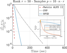
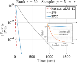
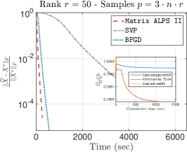
Figure 3: Convergence performance of algorithms under comparison w.r.t. $\tfrac{\|\widehat{X}-X^{\star}\|_{F}}{\|X^{\star}\|_{F}}$ vs. the total execution time. Top row corresponds to dimensions $m=n=1024$; bottom row corresponds to dimensions $m=2048,~{}n=4096$. Details on problem configuration are given on plots’ title. For all cases, we used $\mathcal{A}$ as noiselets and $r=50$.

To further show how the performance of each algorithms scales as dimension increases, we provide aggregated results in Tables 3-4. Observe that BFGD is one order of magnitude faster than the rest non-convex factorization algorithms. Table 5 shows the median time per iteration, spent by each algorithm, for both problem instances and $C=3$. Observe that SVP requires one order of magnitude more time to complete one iteration, mostly due to the SVD step. In stark contrast, all factorization-based approaches spend less time per iteration, as was expected by the discussion in Section 6.1.

		$r=50$, $C=10$				$r=50$, $C=5$				$r=50$, $C=3$
Algorithm		$\tfrac{\|\widehat{X}-X^{\star}\|_{F}}{\|X^{\star}\|_{F}}$		Total time		$\tfrac{\|\widehat{X}-X^{\star}\|_{F}}{\|X^{\star}\|_{F}}$		Total time		$\tfrac{\|\widehat{X}-X^{\star}\|_{F}}{\|X^{\star}\|_{F}}$		Total time
SVP		6.8623e-07		29.0563		3.7511e-06		115.9088		5.7362e-04		517.5673
Procrustes Flow		8.6546e-03		291.0442		5.4418e-01		236.4496		1.0831e+00		223.2486
SparseApproxSDP		1.5616e-02		223.1522		4.9298e-02		158.5459		3.8444e-01		141.5906
GuaranteedMC		9.2570e-01		95.5135		9.3168e-01		260.8471		9.3997e-01		59.4259
BFGD		7.0830e-07		16.2818		2.3199e-06		35.3988		1.1575e-05		157.6610

Table 3: Summary of comparison results for reconstruction and efficiency. Here, $m=n=1024$, resulting into $1,048,576$ variables to optimize, and $\mathcal{A}$ is a noiselet-based subsampled linear map. The number of samples $p$ satisfies $p=C\cdot n\cdot r$ for various values of constant $C$. Time reported is in seconds.

		$r=50$, $C=10$				$r=50$, $C=5$				$r=50$, $C=3$
Algorithm		$\tfrac{\|\widehat{X}-X^{\star}\|_{F}}{\|X^{\star}\|_{F}}$		Total time		$\tfrac{\|\widehat{X}-X^{\star}\|_{F}}{\|X^{\star}\|_{F}}$		Total time		$\tfrac{\|\widehat{X}-X^{\star}\|_{F}}{\|X^{\star}\|_{F}}$		Total time
SVP		1.4106e-06		349.7021		5.6928e-06		1144.7489		1.4110e-04		4703.2012
Procrustes Flow		2.1174e-01		1909.4748		8.7944e-01		1653.7020		1.1088e+00		1692.7454
SparseApproxSDP		1.4268e-02		1484.2220		2.8839e-02		1187.5287		1.7544e-01		1165.4210
GuaranteedMC		1.0114e+00		69.2279		1.0465e+00		53.1636		1.1147e+00		78.2304
BFGD		6.9736e-07		103.8387		1.7946e-06		195.5111		6.6787e-06		561.8248

Table 4: Summary of comparison results for reconstruction and efficiency. Here, $m=2048,~{}n=4096$, resulting into $8,388,608$ variables to optimize, and $\mathcal{A}$ is a noiselet-based subsampled linear map. The number of samples $p$ satisfies $p=C\cdot n\cdot r$ for various values of constant $C$. Time reported is in seconds.

		$m=n=1024$, $C=3$		$m=2048,~{}n=4096$, $C=3$
Algorithm		Median time per iter.		Median time per iter.
SVP		1.604e-01		1.040e+00
Procrustes Flow		5.871e-02		4.525e-01
SparseApproxSDP		3.407e-02		3.001e-01
GuaranteedMC		7.142e-02		4.059e-01
BFGD		5.337e-02		3.981e-01

Table 5: Median time per iteration. Time reported is in seconds.

Results using specific initialization. In this case, we study the effect of initialization in the convergence performance of each algorithm. To do so, we focus only on the factorization-based algorithms: Procrustes Flow, GuaranteedMC, and BFGD. We consider two problem cases: $(i)$ all these schemes use our initialization procedure, and $(ii)$ each algorithm uses its own suggested initialization procedure. The results are depicted in Tables 6-7, respectively.

Using our initialization procedure for all algorithms, we observe that both Procrustes Flow and GuaranteedMC schemes can compute an approximation $\widehat{X}$ such that $\tfrac{\|\widehat{X}-X^{\star}\|_{F}}{\|X^{\star}\|_{F}}>10^{-1}$. In contrast, our approach achieves a solution $\widehat{X}$ that is close to the stopping criterion, i.e., $\tfrac{\|\widehat{X}-X^{\star}\|_{F}}{\|X^{\star}\|_{F}}\approx 10^{-6}$.

		$m=n=1024$, $C=10$, $r=50$				$m=n=1024$, $C=10$, $r=5$
Algorithm		$\tfrac{\|\widehat{X}-X^{\star}\|_{F}}{\|X^{\star}\|_{F}}$		Total time		$\tfrac{\|\widehat{X}-X^{\star}\|_{F}}{\|X^{\star}\|_{F}}$		Total time
Procrustes Flow		2.2703e+01		281.2095		4.0432e+01		192.0993
GuaranteedMC		9.2570e-01		96.8512		4.7646e-01		2.4792
BFGD		3.7055e-06		52.5205		8.1246e-06		65.4926

Table 6: Summary of results of factorization algorithms using our proposed initialization.

Using different initialization schemes per algorithm, the results are depicted in Table 7. We remind that GuaranteedMC is designed for matrix completion tasks, where the linear operator is a selection mask of the entries. Observe that Procrustes Flow’s performance improves significantly by using their proposed initialization: the idea is to perform SVP iterations to get to a good initial point; then switch to non-convex factored gradient descent for low per-iteration complexity. However, this initialization is computationally expensive: Procrustes Flow might end up performing several SVP iterations. This can be observed e.g., in the case $m=n=1024,~{}r=5$ and comparing the results in Tables 6-7: for this case, Procrustes Flow performs $T=4000$ iterations when our initialization is used and spends $\sim 200$ seconds, while in Table 7 it performs $T\ll 4000$ iterations, at least $20\%$ of them using SVP, and consumes $\sim 2000$ seconds.

		$m=n=1024$, $C=10$, $r=50$				$m=n=1024$, $C=10$, $r=5$
Algorithm		$\tfrac{\|\widehat{X}-X^{\star}\|_{F}}{\|X^{\star}\|_{F}}$		Total time		$\tfrac{\|\widehat{X}-X^{\star}\|_{F}}{\|X^{\star}\|_{F}}$		Total time
Procrustes Flow		3.2997e-05		390.6830		8.5741e-04		2017.7942
GuaranteedMC		9.2570e-01		114.9332		1.0114e+00		68.1775
BFGD		3.6977e-06		64.2690		3.1471e-06		74.2345
		$m=2048,n=4096$, $C=10$, $r=50$				$m=2048,n=4096$, $C=10$, $r=5$
Algorithm		$\tfrac{\|\widehat{X}-X^{\star}\|_{F}}{\|X^{\star}\|_{F}}$		Total time		$\tfrac{\|\widehat{X}-X^{\star}\|_{F}}{\|X^{\star}\|_{F}}$		Total time
Procrustes Flow		4.9896e-02		265.2787		4.2263e-02		1497.6867
GuaranteedMC		4.7646e-01		4.0752		1.0302e+00		35.0559
BFGD		8.1381e-06		83.3411		5.8428e-06		379.1430

Table 7: Summary of results of factorization algorithms using each algorithm’s proposed initialization.

6.4 Image Denoising as Matrix Completion Problem

In this example, we consider the matrix completion setting for an image denoising task: In particular, we observe a limited number of pixels from the original image and perform a low rank approximation based only on the set of measurements—similar experiments can be found in [65, 100]. We use real data images: While the true underlying image might not be low-rank, we apply our solvers to obtain low-rank approximations.

Figures 4-6 depict the reconstruction results for three image cases. In all cases, we compute the best $100$-rank approximation of each image (see e.g., the top middle image in Figure 4, where the full set of pixels is observed) and we observe only the $35\%$ of the total number of pixels, randomly selected—a realization is depicted in the top right plot in Figure 4. Given a fixed common tolerance level and the same stopping criterion as before, the top rows of Figures 4-6 show the recovery performance achieved by a range of algorithms under consideration—the peak signal to noise ration (PSNR), depicted in dB, corresponds to median values after 10 Monte-Carlo realizations. Our algorithm shows competitive performance compared to simple gradient descent schemes as SVP and Procrustes Flow, while being a fast and scalable solver. Table 8 contains timing results from 10 Monte Carlo random realizations for all image cases.

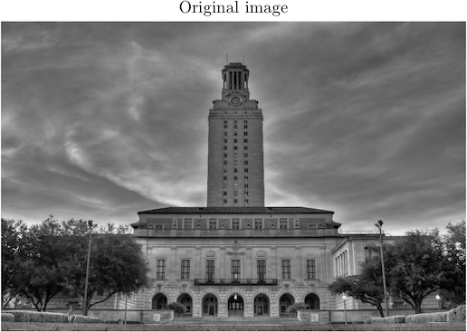
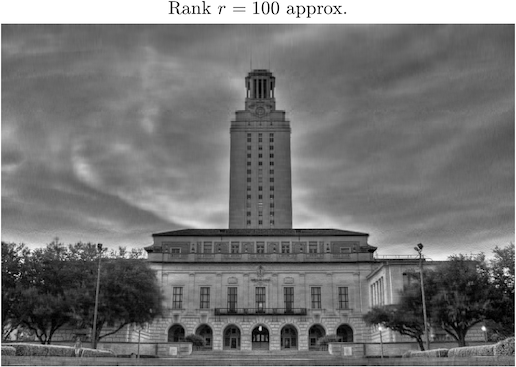
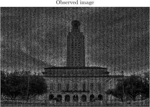
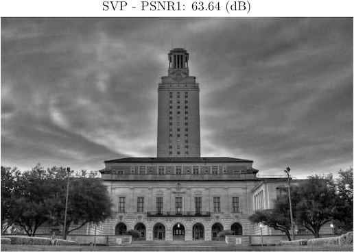
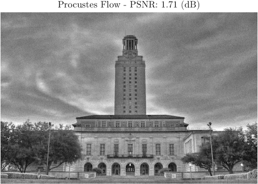
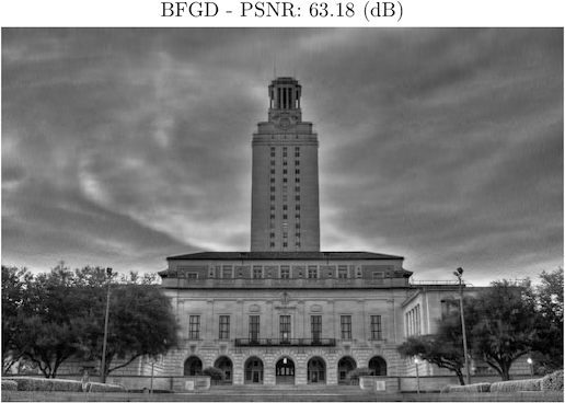
Figure 4: Reconstruction performance in image denoising settings. The image size is $2845\times 4266$ ($12,136,770$ pixels) and the approximation rank is preset to $r=100$. We observe 35% of the pixels of the true image. We depict the median reconstruction error with respect to the true image in dB over 10 Monte Carlo realizations.

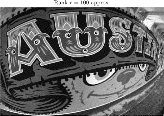
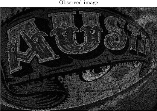
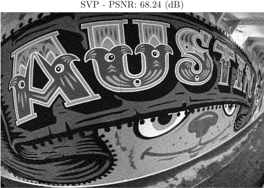
Figure 5: Reconstruction performance in image denoising settings. The image size is $3309\times 4963$ ($16,422,567$ pixels) and the approximation rank is preset to $r=100$. We observe 30% of the pixels of the true image. We depict the median reconstruction error with respect to the true image in dB over 10 Monte Carlo realizations.

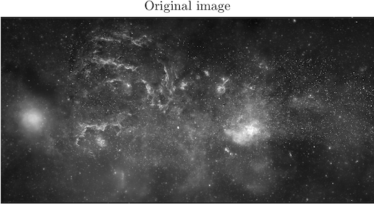
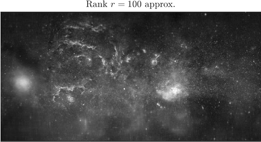
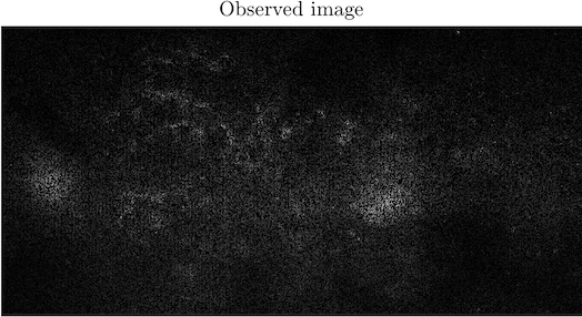
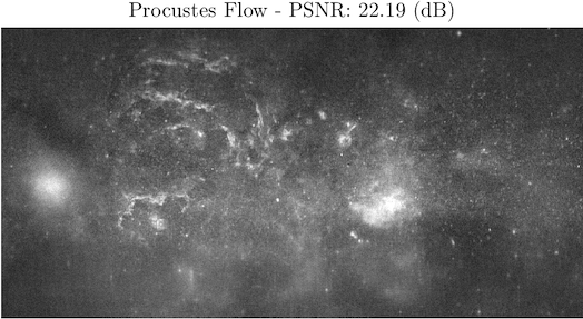
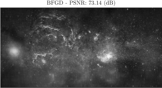
Figure 6: Reconstruction performance in image denoising settings. The image size is $4862\times 9725$ ($47,282,950$ pixels) and the approximation rank is preset to $r=100$. We observe 30% of the pixels of the true image. We depict the median reconstruction error with respect to the true image in dB over 10 Monte Carlo realizations.

		Time (sec.)
Algorithm		UT Campus		Graffiti		Milky way
SVP		5224.1		4154.9		7921.4
Procrustes Flow		5383.4		6501.4		12806.3
BFGD		4062.4		3155.9		9119.6

Table 8: Summary of execution time results for the problem of image denoising. Timings correspond to median values on 10 Monte Carlo random instantiations.

6.5 1-bit Matrix Completion

For this task, we repeat the experiments in [37] and compare BFGD with their proposed schemes. The observational model we consider here satisfies the following principles: We assume $X^{\star}\in\mathbb{R}^{m\times n}$ is an unknown low rank matrix, satisfying $\|X^{\star}\|_{\infty}\leq\alpha,~{}\alpha>0$, from which we observe only a subset of indices $\Omega\subset[m]\times[n]$, according to the following rule:

$$Y_{i,j}=\left\{\begin{array}[]{ll}+1&\mbox{with probability }\sigma(X^{\star}_{i,j})\\ -1&\mbox{with probability }1-\sigma(X^{\star}_{i,j})\end{array}\right.\quad\quad\text{for }(i,j)\in\Omega.$$ (26)

Similar to classic matrix completion results, we assume $\Omega$ is chosen uniformly at random, e.g., we assume $\Omega$ follows a binomial model, as in [37]. Two natural choices for $\sigma$ function are: $(i)$ the logistic regression model, where $\sigma(x)=\tfrac{e^{x}}{1+e^{x}}$, and $(ii)$ the probit regression model, where $\sigma(x)=1-\Phi(-x/\sigma)$ for $\Phi$ being the cumulative Gaussian distribution function. Both models correspond to different noise assumptions: in the first case, noise is modeled according to the standard logistic distribution, while in the second case, noise follows standard Gaussian assumptions. Under this model, [37] propose two convex relaxation algorithmic solutions to recover $X^{\star}$: $(i)$ the convex maximum log-likelihood estimator under nuclear norm and infinity norm constraints:

$$\underset{X\in\mathbb{R}^{m\times n}}{\text{minimize}} f(X),$$ (27)

subject to $$\|X\|_{*}\leq\alpha\sqrt{rmn},~{}~{}\|X\|_{\infty}\leq\alpha,$$

and $(ii)$ the the convex maximum log-likelihood estimator under only nuclear norm constraints. In both cases, $f(X)$ satisfies the expression in (7). [37] proposes a spectral projected-gradient descent method for both these criteria; in the case where only nuclear norm constraints are present, SVD routines compute the convex projection onto norm balls, while in the case where both nuclear and infinity norm constraints are present, [37] propose a alternating-direction method of multipliers (ADMM) solution, in order to compute the joint projection onto these sets.

Synthetic experiments. We synthetically construct $X^{\star}\in\mathbb{R}^{m\times n}$, where $m=n=100$, such that $X^{\star}=U^{\star}V^{\star\top}$, where $U^{\star}\in\mathbb{R}^{m\times r}$, $V^{\star}\in\mathbb{R}^{n\times r}$ for $r=1$. The entries of $U^{\star}$, $V^{\star}$ are drawn i.i.d. from $\text{Uni}\left[-\tfrac{1}{2},~{}\tfrac{1}{2}\right]$. Moreover, according to [37], we scale $X^{\star}$ such that $\|X^{\star}\|_{\infty}=1$. Then, we observe $Y\in\mathbb{R}^{m\times n}$ according to (26), where $|\Omega|=\tfrac{1}{4}\cdot mn$. we consider the probit regression model with additive Gaussian noise, with variance $\sigma^{2}$.

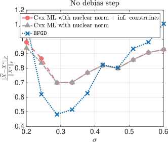
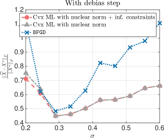
Figure 7: Comparison of 1-bit matrix procedures. Left panel: Output of (27) is not projected onto rank-$r$ set. Right panel: Output of (27) is projected onto rank-$r$ set.

Figure 7 depicts the recovery performance of BFGD, as compared to variants of (27) in [37]. We consider their performance over different noise levels w.r.t. the normalized Frobenius norm distance $\tfrac{\|\widehat{X}-X^{\star}\|_{F}}{\|X^{\star}\|_{F}}$. As noted in [37], the performance of all algorithms is poor when $\sigma$ is too small or too large, while in between, for moderate noise levels, we observe better performance for all approaches.

By default, in all problem settings, we observe that the estimate of (27) is not of low rank: to compute the closest rank-$r$ approximation to that, we further perform a debias step via truncated SVD. The effect of the debias step is better illustrated in Figure 7, focusing on the differences between left and right plot: without such step, BFGD has a better performance in terms of $\tfrac{\|\widehat{X}-X^{\star}\|_{F}}{\|X^{\star}\|_{F}}$, within the “sweet” range of noise levels, compared to the convex analog in (27). Applying the debias step, both approaches have comparable performance, with that of (27) being slightly better.

Perhaps somewhat surprisingly, the performance of BFGD, in terms of estimating the correct sign pattern of the entries, is better than that of [37], even with the debias step. Figure 8 (left panel) illustrates the observed performances for various noise levels.

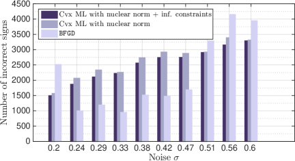
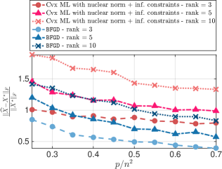
Figure 8: Left panel: Comparison of 1-bit matrix procedures w.r.t. sign pattern estimation. Right panel: Recovery of $X^{\star}$ from $p=C\cdot n^{2}$ measurements. $X^{\star}$ is designed to be low rank: $r=3,5$ and $10$. x-axis represents $C$ for various values.

Finally, we study the performance of the algorithms under consideration as a function of the number of measurements, for fixed settings of dimensions $m=n=200$ and noise level $\sigma=0.244$. By the discussion above, such noise level leads to good performance from all schemes. We considered matrices $X^{\star}$ with rank $r\in\left\{3,~{}5,~{}10\right\}$ and generate $p=C\cdot n^{2}$, over a wide range of $0<C<1$. Figure 8 (right panel) shows the performance of BFGD and the approach for (27) in [37], in terms of the relative Frobenius norm of the error. All approaches do poorly when there are only $p<0.35\cdot n^{2}$ measurements, since this is near the noiseless information-theoretic limit. For higher numbers of measurements, the non-convex approach in BFGD returns more reasonable solutions and outperforms convex approaches, taking advantage of the prior knowledge on low-rankness of the solution.

Recommendation system using the MovieLens data set. We compare 1-bit matrix completion solvers on the 100k MovieLens data set. To do so, we repeat the experiment in Section 4.3 of [37]: we use the MovieLens 100k, which consists of 100k movie ratings, from 1000 users on 1700 movies. Each user entry denotes the movie rating, ranging from 1 to 5. To convert this data set into 1-bit measurements, we convert these ratings to binary observations by comparing each rating to the average rating for the entire data set (which is approximately 3.5), according to [37]. To evaluate the performance of the algorithms, we assume part of the observed ratings as unobserved (5k of them) and check if the estimate of $X^{\star}$, $\widehat{X}$, predicts the sign of these ratings. We perform ML estimation using logistic function $\sigma(x)=\tfrac{e^{x}}{1+e^{x}}$ in $f$.

We compare the following algorithms: $(i)$ the spectral projected gradient descent (SPG) implementation of (27) in [37] for 1-bit matrix completion, $(ii)$ the standard matrix completion implementation TFOCS [12], where we observe the unquantized data set (actual values), $(iii)$ BFGD for various values of rank parameter $r$. The results are shown Table 9 over 10 Monte Carlo realizations (i.e., we randomly selected 5k ratings as test sets and solved the problem for different runs of the algorithms). The values in Table 9 denote the accuracy in predicting whether the unobserved ratings are above or below the average rating of 3.5. BFGD shows competitive performance, compared to convex approaches. Moreover, setting the parameter $r$ is an “easier” and more intuitive task: our algorithm administers precise control on the rankness of the solution, which might lead to further interpretation of the results. Convex approaches lack of this property: the mapping between the regularization parameters and the number of rank-1 components in the extracted solution is highly non-linear. At the same time, BFGD shows much faster convergence to a good solution, which constitutes it a preferable algorithmic solution for large scale applications.

		Ratings (%)										Overall (%)		Time (sec)
Algorithm		1		2		3		4		5
SPG ($\alpha\sqrt{r}=0.32$)		73.7		68.4		52.5		74.9		91.0		71.3		79.5
SPG ($\alpha\sqrt{r}=4.64$)		77.2		71.0		58.5		72.5		86.9		71.8		213.4
SPG ($\alpha\sqrt{r}=10.00$)		76.2		71.3		58.3		71.0		85.7		71.0		491.8
TFOCS		70.4		69.4		59.2		39.1		59.4		64.8		42.3
BFGD ($r=3$)		79.4		74.5		56.9		72.5		88.2		72.2		25.4
BFGD ($r=5$)		79.0		72.4		56.8		71.6		86.2		71.2		27.5
BFGD ($r=10$)		77.6		75.0		57.5		70.5		84.1		70.9		30.3

Table 9: Summary of results for the problem of 1-bit matrix completio on MovieLens data set. Individual and overall ratings correspond to percentages of signs correctly estimated (+1 corresponds to original rating above 3.5, -1 corresponds to original rating below 3.5). Timings correspond to median values on 10 Monte Carlo random instantiations.

Appendix A Appendix

Proof of (18)$\Rightarrow$(17) Let $R^{\star}_{t}$ be the $r\times r$ orthogonal matrix such that ${\rm{\textsc{Dist}}}(U_{t},V_{t};X^{\star}_{r})=\left\|{W_{t}-W^{\star}R^{\star}_{t}}\right\|_{F}$. By the triangle inequality, we have

$$\|W_{t}\|_{2} =\|W_{t}-W^{\star}R^{\star}_{t}+W^{\star}R_{t}^{\star}\|_{2}\stackrel{{\scriptstyle(i)}}{{\leq}}\|W^{\star}R^{\star}_{t}\|_{2}+\|W_{t}-W^{\star}R^{\star}_{t}\|_{2}$$

$$\stackrel{{\scriptstyle(ii)}}{{\leq}}\|W^{\star}\|_{2}+\tfrac{\sqrt{2}\sigma_{r}\left(X^{\star}_{r}\right)^{\nicefrac{{1}}{{2}}}}{10}$$

$$\stackrel{{\scriptstyle(iii)}}{{\leq}}\|W^{\star}\|_{2}+\tfrac{\sigma_{r}\left(W^{\star}\right)}{10}$$

$$\leq\tfrac{11}{10}\cdot\|W^{\star}\|_{2}$$ (28)

where $(i)$ is due to triangle inequality, $(ii)$ is due to Assumption A.1 $(iii)$ is due to the fact that $\sqrt{2}\cdot\sigma_{r}(X^{\star}_{r})^{\nicefrac{{1}}{{2}}}=\sigma_{r}(W^{\star})$ and $\kappa\geq 1$. The above bound holds for every $t=0,1,\ldots$.

On the other hand, we have:

$$\|W_{0}\|_{2} =\|W_{0}-W^{\star}R^{\star}_{t}+W^{\star}R^{\star}\|_{2}\stackrel{{\scriptstyle(i)}}{{\geq}}\|W^{\star}R^{\star}_{t}\|_{2}-\|W_{0}-W^{\star}R^{\star}_{t}\|_{2}$$

$$\geq\|W^{\star}\|_{2}-\tfrac{\sqrt{2}\sigma_{r}\left(X^{\star}_{r}\right)^{\nicefrac{{1}}{{2}}}}{10}$$

$$\geq\|W^{\star}\|_{2}-\tfrac{\sigma_{1}\left(W^{\star}\right)}{10}$$

$$\geq\tfrac{9}{10}\cdot\|W^{\star}\|_{2}$$ (29)

Combining (A) and (A), we obtain:

$$\|W_{t}\|_{2}\leq\tfrac{11}{10}\cdot\|W^{\star}\|_{2}\leq\tfrac{11}{9}\|W_{0}\|_{2}\Longrightarrow\tfrac{81}{121}\cdot\|W_{t}\|_{2}^{2}\leq\|W_{0}\|_{2}^{2}$$

and, finally,

$$\tfrac{1}{8\cdot\max\{L,~{}L_{g}\}\cdot\|W_{t}\|_{2}^{2}}=\tfrac{1}{8\cdot\tfrac{121}{81}\cdot\max\{L,~{}L_{g}\}\cdot\tfrac{81}{121}\cdot\|W_{t}\|_{2}^{2}}\geq\tfrac{1}{12\cdot\max\{L,~{}L_{g}\}\cdot\|W_{0}\|_{2}^{2}}$$

$\blacksquare$

Proof of (19)$\Rightarrow$(15) We have

$$\|\nabla f(U_{t}V_{t}^{\top})\|_{2} \leq\|\nabla f(U_{0}V_{0}^{\top})\|_{2}+\|\nabla f(U_{t}V_{t}^{\top})-\nabla f(U_{0}V_{0}^{\top})\|_{2}$$

$$\stackrel{{\scriptstyle(i)}}{{\leq}}\|\nabla f(U_{0}V_{0}^{\top})\|_{2}+L\|U_{t}V_{t}^{\top}-U_{0}V_{0}^{\top}\|_{F}$$

$$\stackrel{{\scriptstyle(ii)}}{{\leq}}\|\nabla f(U_{0}V_{0}^{\top})\|_{2}+L\|U_{t}V_{t}^{\top}-U^{\star}{V^{\star}}^{\top}\|_{F}+L\|U_{0}V_{0}^{\top}-U^{\star}{V^{\star}}^{\top}\|_{F}$$ (30)

where $(i)$ is due to the fact that $f$ is $L$-smooth and, $(ii)$ holds by adding and subtracting $U^{\star}V^{\star\top}$ and then applying triangle inequality. To bound the last two terms on the right hand side, we observe:

$$\|U_{t}V_{t}^{\top}-U^{\star}{V^{\star}}^{\top}\|_{F} =\|U_{t}V_{t}^{\top}-U^{\star}RV_{t}^{\top}+U^{\star}RV_{t}^{\top}-U^{\star}RR^{\top}{V^{\star}}^{\top}\|_{F}$$

$$\stackrel{{\scriptstyle(i)}}{{\leq}}\left\|{U^{\star}R}\right\|_{2}\cdot\left\|{V_{t}-V^{\star}R}\right\|_{F}+\left\|{V_{t}}\right\|_{2}\cdot\left\|{U_{t}-U^{\star}R}\right\|_{F}$$

$$\leq\left(\left\|{U^{\star}}\right\|_{2}+\left\|{V_{t}}\right\|_{2}\right)\cdot{\rm{\textsc{Dist}}}(U_{t},V_{t};X^{\star}_{r})$$

$$\stackrel{{\scriptstyle(ii)}}{{\leq}}\frac{21}{10}\cdot\left\|{W^{\star}}\right\|_{2}\cdot\frac{\sigma_{r}(W^{\star})}{10}$$

$$\leq\frac{7}{10}\cdot\left\|{W_{0}}\right\|_{2}^{2}$$

where $(i)$ is due to the triangle and Cauchy-Schwartz inequalities, $(ii)$ is by Assumption A1 and (A). Similarly, one can show that $\|U_{0}V_{0}^{\top}-U^{\star}{V^{\star}}^{\top}\|_{F}\leq\frac{7}{10}\cdot\left\|{W_{0}}\right\|_{2}^{2}$. Thus, (30) becomes:

$$\|\nabla f(U_{0}V_{0}^{\top})\|_{2}\geq\|\nabla f(U_{t}V_{t}^{\top})\|_{2}-\frac{3L}{2}\left\|{W_{0}}\right\|_{2}^{2}$$ (31)

Applying (A), (A), and the above bound, we obtain the desired result. $\blacksquare$

Appendix B Appendix

For clarity, we omit the subscript $t$, and use $(U,~{}V)$ to denote the current estimate and $(U^{+},V^{+})$ the next estimate. Further, we abuse the notation by denoting $\nabla g\triangleq\nabla g(U^{\top}U-V^{\top}V)$, where the gradient is taken over both $U$ and $V$. We denote the stacked matrices of $(U,V)$ and their variants as follows:

$$W=\begin{bmatrix}U\\ V\end{bmatrix},~{}W^{+}=\begin{bmatrix}U^{+}\\ V^{+}\end{bmatrix},~{}W^{\star}=\begin{bmatrix}U^{\star}\\ V^{\star}\end{bmatrix}.$$

Observe that $W,W^{+},W^{\star}\in\mathbb{R}^{(m+n)\times r}$. Then, the main recursion of BFGD in Algorithm 1 can be succinctly written as

$${W}^{\scalebox{0.7}{+}}=W-\widehat{\eta}\nabla_{W}(f+\tfrac{1}{2}g),$$

where

$$\nabla_{W}(f+\tfrac{1}{2}g)=\begin{bmatrix}\nabla_{U}f(UV^{\top})+\tfrac{1}{2}\nabla_{U}g\\ \nabla_{V}f(UV^{\top})+\tfrac{1}{2}\nabla_{V}g\\ \end{bmatrix}=\begin{bmatrix}\nabla f(UV^{\top})V+\tfrac{1}{2}U\nabla g\\ \nabla f(UV^{\top})^{\top}U-\tfrac{1}{2}V\nabla g\\ \end{bmatrix}.$$

In the above formulations, we use as regularizer of $g$ function $\lambda=\tfrac{1}{2}$.

Our discussion below is based on the Assumption A.1, where:

$${\rm{\textsc{Dist}}}(U,V;X^{\star}_{r})\leq\frac{\sqrt{2}\cdot\sigma_{r}(X^{\star}_{r})^{1/2}}{10\sqrt{\kappa}}=\frac{\sigma_{r}(W^{\star})}{10\sqrt{\kappa}},$$ (32)

holds for the current iterate. The last equality is due to the fact that $\sigma_{r}(W^{\star})=\sqrt{2}\cdot\sigma_{r}(X^{\star}_{r})^{1/2}$, for $(U^{\star},V^{\star})$ with “equal footing”. For the initial point $(U_{0},V_{0})$, (32) holds by the assumption of the theorem. Since the right hand side is fixed, (32) holds for every iterate, as long as ${\rm{\textsc{Dist}}}(U,V;X^{\star}_{r})$ decreases.

To show this, let $R\in O_{r}$ be the minimizing orthogonal matrix such that ${\rm{\textsc{Dist}}}(U,V;X^{\star}_{r})=\left\|{W-W^{\star}R}\right\|_{F}$; here, $O_{r}$ denotes the set of $r\times r$ orthogonal matrices such that $R^{\top}R=I$. Then, the decrease in distance can be lower bounded by

$${\rm{\textsc{Dist}}}(U,V;X^{\star}_{r})^{2} -{\rm{\textsc{Dist}}}({U}^{\scalebox{0.7}{+}},{V}^{\scalebox{0.7}{+}};X^{\star}_{r})^{2}$$

$$=\left\|{W-W^{\star}R}\right\|_{F}^{2}-\min_{Q\in O_{r}}\left\|{W^{+}-W^{\star}Q}\right\|_{F}^{2}$$

$$\geq\left\|{W-W^{\star}R}\right\|_{F}^{2}-\left\|{W^{+}-W^{\star}R}\right\|_{F}^{2}$$

$$=2\widehat{\eta}\cdot\left\langle\nabla_{W}(f+\tfrac{1}{2}g),W-W^{\star}R\right\rangle-\widehat{\eta}^{2}\cdot\left\|{\nabla_{W}(f+\tfrac{1}{2}g)}\right\|_{F}^{2}$$ (33)

where the last equality is obtaining by substituting $W^{+}$, according to its definition above. To bound the first term on the right hand side, we use the following lemma; the proof is provided in Section B.

Lemma B.1 (Descent lemma).

Suppose (32) holds for $W$. Let $\mu_{\min}=\min\left\{\mu,~{}\mu_{g}\right\}$ and $L_{\max}=\max\left\{L,~{}L_{g}\right\}$ for $(\mu,L)$ and $(\mu_{g},L_{g})$ the strong convexity and smoothness parameters pairs for $f$ and $g$, respectively. Then, the following inequality holds:

$$\left\langle\nabla_{W}(f+\tfrac{1}{2}g),W-W^{\star}R\right\rangle \geq\tfrac{\mu_{\min}\cdot\sigma_{r}(W^{\star})^{2}}{20}\left\|{W-W^{\star}R}\right\|_{F}^{2}+\tfrac{1}{4L_{\max}}\left\|{\nabla f(UV^{\top})}\right\|_{F}^{2}$$

$$+\tfrac{1}{16L_{\max}}\left\|{\nabla g}\right\|_{F}^{2}-\tfrac{L}{2}\left\|{X^{\star}-X^{\star}_{r}}\right\|_{F}^{2}$$ (34)

For the second term on the right hand side of (B), we obtain the following upper bound:

$$\left\|{\nabla_{W}(f+\tfrac{1}{2}g)}\right\|_{F}^{2} =\left\|\begin{bmatrix}\nabla f(UV^{\top})V+\tfrac{1}{2}U\nabla g\\ \nabla f(UV^{\top})^{\top}U-\tfrac{1}{2}V\nabla g\\ \end{bmatrix}\right\|_{F}^{2}$$

$$=\left\|{\nabla f(UV^{\top})V+\tfrac{1}{2}U\nabla g}\right\|_{F}^{2}+\left\|{\nabla f(UV^{\top})^{\top}U-\tfrac{1}{2}V\nabla g}\right\|_{F}^{2}$$

$$\stackrel{{\scriptstyle(a)}}{{\leq}}2\left\|{\nabla f(UV^{\top})V}\right\|_{F}^{2}+\tfrac{1}{2}\left\|{U\nabla g}\right\|_{F}^{2}+2\left\|{\nabla f(UV^{\top})^{\top}U}\right\|_{F}^{2}+\tfrac{1}{2}\left\|{V\nabla g}\right\|_{F}^{2}$$

$$=2\left\|{\nabla f(UV^{\top})V}\right\|_{F}^{2}+2\left\|{\nabla f(UV^{\top})^{\top}U}\right\|_{F}^{2}+\tfrac{1}{2}\left\|{W\nabla g}\right\|_{F}^{2}$$

$$\stackrel{{\scriptstyle(b)}}{{\leq}}2\left\|{\nabla f(UV^{\top})}\right\|_{F}^{2}\cdot\left(\left\|{U}\right\|_{2}^{2}+\left\|{V}\right\|_{2}^{2}\right)+\tfrac{1}{2}\left\|{W}\right\|_{2}^{2}\left\|{\nabla g}\right\|_{F}^{2}$$

$$\stackrel{{\scriptstyle(c)}}{{\leq}}\left(4\left\|{\nabla f(UV^{\top})}\right\|_{F}^{2}+\tfrac{1}{2}\left\|{\nabla g}\right\|_{F}^{2}\right)\cdot\left\|{W}\right\|_{2}^{2},$$ (35)

where $(a)$ follows from the fact $\left\|{A+B}\right\|_{F}^{2}\leq 2\left\|{A}\right\|_{F}^{2}+2\left\|{B}\right\|_{F}^{2}$, $(b)$ is due to the fact $\left\|{AB}\right\|_{F}\leq\left\|{A}\right\|_{F}\cdot\left\|{B}\right\|_{2}$, and $(c)$ follows from the observation that $\left\|{U}\right\|_{2},\left\|{V}\right\|_{2}\leq\left\|{W}\right\|_{2}$.

Plugging (B.1) and (B) in (B), we get

$${\rm{\textsc{Dist}}}(U,V;X^{\star}_{r})^{2} -{\rm{\textsc{Dist}}}({U}^{\scalebox{0.7}{+}},{V}^{\scalebox{0.7}{+}};X^{\star}_{r})^{2}$$

$$\geq 2\widehat{\eta}\cdot\left\langle\nabla_{W}(f+\tfrac{1}{2}g),W-W^{\star}R\right\rangle-\widehat{\eta}^{2}\cdot\left\|{\nabla_{W}(f+\tfrac{1}{2}g)}\right\|_{F}^{2}$$

$$\geq\tfrac{\widehat{\eta}\cdot\mu_{\min}\cdot\sigma_{r}(W^{\star})^{2}}{10}{\rm{\textsc{Dist}}}(U,V;X^{\star}_{r})^{2}-\widehat{\eta}L\left\|{X^{\star}-X^{\star}_{r}}\right\|_{F}^{2}$$

$$=\tfrac{\widehat{\eta}\cdot\mu_{\min}\cdot\sigma_{r}(X^{\star}_{r})}{5}{\rm{\textsc{Dist}}}(U,V;X^{\star}_{r})^{2}-\widehat{\eta}L\left\|{X^{\star}-X^{\star}_{r}}\right\|_{F}^{2}$$

where we use the fact that $\sigma_{r}(W^{\star})=\sqrt{2}\cdot\sigma_{r}(X^{\star}_{r})^{1/2}$.

The above lead to the following recursion:

$${\rm{\textsc{Dist}}}({U}^{\scalebox{0.7}{+}},{V}^{\scalebox{0.7}{+}};X^{\star}_{r})^{2}\leq\gamma_{t}\cdot{\rm{\textsc{Dist}}}(U,V;X^{\star}_{r})^{2}+\widehat{\eta}L\left\|{X^{\star}-X^{\star}_{r}}\right\|_{F}^{2},$$

where $\gamma_{t}=1-\tfrac{\widehat{\eta}\cdot\mu_{\min}\cdot\sigma_{r}(X^{\star}_{r})}{5}$. By the definition of $\widehat{\eta}$ in (18), we further have:

$$\gamma_{t} =1-\tfrac{\mu_{\min}\cdot\sigma_{r}(X^{\star}_{r})}{40\cdot L_{\max}\cdot\|W\|_{2}^{2}}$$

$$\stackrel{{\scriptstyle(i)}}{{\geq}}1-\tfrac{\mu_{\min}\cdot\sigma_{r}(X^{\star}_{r})}{40\cdot L_{\max}\cdot\tfrac{100}{81}\cdot\|W^{\star}\|_{2}^{2}}$$

$$\stackrel{{\scriptstyle(ii)}}{{\geq}}1-\tfrac{\mu_{\min}}{17\cdot L_{\max}}\cdot\tfrac{\sigma_{r}(X^{\star}_{r})}{\sigma_{1}(X^{\star}_{r})}$$

where $(i)$ is by using (A) that connects $\|W\|_{2}$ with $\|W^{\star}\|_{2}$ as $\|W\|_{2}\geq\tfrac{9}{10}\|W^{\star}\|_{2}$, and $(ii)$ is due to the fact $\|W^{\star}\|_{2}=\sqrt{2}\cdot\sigma_{1}(X^{\star}_{r})^{1/2}$. $\blacksquare$

B.1. Proof of Lemma B.1

Before we step into the proof, we require a few more notations for simpler presentation of our ideas. We use another set of stacked matrices $Y=\begin{bmatrix}U\\ -V\end{bmatrix},~{}Y^{\star}=\begin{bmatrix}U^{\star}\\ -V^{\star}\end{bmatrix}.$ The error of the current estimate from the closest optimal point is denoted by the following $\Delta_{\times}$ matrix structures:

$$\Delta_{U}=U-U^{\star}R,\quad\Delta_{V}=V-V^{\star}R,\quad\Delta_{W}=W-W^{\star}R,\quad\Delta_{Y}=Y-Y^{\star}R.$$

For our proof, we can write

$$\left\langle\nabla_{W}(f+\tfrac{1}{2}g),W-W^{\star}R\right\rangle =\underbrace{\left\langle\nabla f(UV^{\top})V,U-U^{\star}R\right\rangle+\left\langle\nabla f(UV^{\top})^{\top}U,V-V^{\star}R\right\rangle}_{(A)}$$

$$\quad\quad\quad\quad\quad\quad\quad\quad\quad\quad\quad+\tfrac{1}{2}\cdot\left(\underbrace{\left\langle U\nabla g,U-U^{\star}R\right\rangle-\left\langle V\nabla g,V-V^{\star}R\right\rangle}_{(B)}\right)$$

For (A), we have

$$(A) =\left\langle\nabla f(UV^{\top})V,U-U^{\star}R\right\rangle+\left\langle\nabla f(UV^{\top})^{\top}U,V-V^{\star}R\right\rangle$$

$$=\left\langle\nabla f(UV^{\top}),UV^{\top}-U^{\star}{V^{\star}}^{\top}\right\rangle+\left\langle\nabla f(UV^{\top}),\Delta_{U}\Delta_{V}^{\top}\right\rangle$$ (36)

$$\geq\frac{\mu}{2}\underbrace{\left\|{UV^{\top}-U^{\star}{V^{\star}}^{\top}}\right\|_{F}^{2}}_{(A1)}+\frac{1}{2L}\underbrace{\left\|{\nabla f(UV^{\top})}\right\|_{F}^{2}}_{(A2)}-\frac{L}{2}\underbrace{\left\|{X^{\star}-X^{\star}_{r}}\right\|_{F}^{2}}_{(A3)}-\underbrace{\left\|{\nabla f(UV^{\top})}\right\|_{2}\cdot\left\|{\Delta_{W}}\right\|_{F}^{2}}_{(A4)}$$

where, for the second term in (36), we use the fact that

$$\left\langle\nabla f(UV^{\top}),\Delta_{U}\Delta_{V}^{\top}\right\rangle\geq-\left|\left\langle\nabla f(UV^{\top}),\Delta_{U}\Delta_{V}^{\top}\right\rangle\right|=-\left|\left\langle\nabla f(UV^{\top})\Delta_{V},\Delta_{U}\right\rangle\right|,$$

the Cauchy-Schwarz inequality and the fact that $\|\Delta_{U}\|_{F},\|\Delta_{V}\|_{F}\leq\|\Delta_{W}\|_{F}$; the first term in (36) follows from:

$$\left\langle\nabla f(UV^{\top}),UV^{\top}-U^{\star}{V^{\star}}^{\top}\right\rangle\stackrel{{\scriptstyle(i)}}{{\geq}}f(UV^{\top})-f(U^{\star}{V^{\star}}^{\top})+\frac{\mu}{2}\left\|{UV^{\top}-U^{\star}{V^{\star}}^{\top}}\right\|_{F}^{2}$$

$$\stackrel{{\scriptstyle(ii)}}{{=}}(f(UV^{\top})-f(X^{\star}))-(f(U^{\star}{V^{\star}}^{\top})-f(X^{\star}))+\frac{\mu}{2}\left\|{UV^{\top}-U^{\star}{V^{\star}}^{\top}}\right\|_{F}^{2}$$

$$\stackrel{{\scriptstyle(iii)}}{{\geq}}\frac{1}{2L}\left\|{\nabla f(UV^{\top})}\right\|_{F}^{2}-\frac{L}{2}\left\|{X^{\star}-U^{\star}{V^{\star}}^{\top}}\right\|_{F}^{2}+\frac{\mu}{2}\left\|{UV^{\top}-U^{\star}{V^{\star}}^{\top}}\right\|_{F}^{2}.$$

where $(i)$ is due to the $\mu$-strong convexity of $f$, $(ii)$ is by adding and subtracting $f(X^{\star})$; observe that $f(X^{\star})=f(U^{\star}{V^{\star}}^{\top})$ if and only if $\text{rank}(X^{\star})=r$, and $(iii)$ is due to the $L$-smoothness of $f$ and the fact that $\nabla f(X^{\star})=0$ (for the middle term), and due to the inequality [81, eq. (2.1.7)] (for the first term):

$$f(X)+\langle\nabla f(X),Y-X\rangle+\tfrac{1}{2L}\cdot\|\nabla f(X)-\nabla f(Y)\|_{F}^{2}\leq f(Y).$$ (37)

For (B), we have

$$(B) =\left\langle Y\nabla g,W-W^{\star}R\right\rangle=\left\langle\nabla g,Y^{\top}W-Y^{\top}W^{\star}R\right\rangle$$

$$=\tfrac{1}{2}\left\langle\nabla g,Y^{\top}W-R^{\top}{Y^{\star}}^{\top}W^{\star}R\right\rangle+\tfrac{1}{2}\left\langle\nabla g,Y^{\top}W-2Y^{\top}W^{\star}R+R^{\top}{Y^{\star}}^{\top}W^{\star}R\right\rangle$$

$$\stackrel{{\scriptstyle(a)}}{{=}}\tfrac{1}{2}\left\langle\nabla g,Y^{\top}W\right\rangle+\tfrac{1}{2}\left\langle\nabla g,Y^{\top}W-Y^{\top}W^{\star}R-R^{\top}{Y^{\star}}^{\top}W+R^{\top}{Y^{\star}}^{\top}W^{\star}R\right\rangle$$

$$=\frac{1}{2}\left\langle\nabla g,U^{\top}U-V^{\top}V\right\rangle+\frac{1}{2}\left\langle\nabla g,\Delta_{Y}^{\top}\Delta_{W}\right\rangle$$ (38)

$$\stackrel{{\scriptstyle(b)}}{{\geq}}\frac{\mu_{g}}{4}\underbrace{\left\|{U^{\top}U-V^{\top}V}\right\|_{F}^{2}}_{(B1)}+\frac{1}{4L_{g}}\underbrace{\left\|{\nabla g}\right\|_{F}^{2}}_{(B2)}-\frac{1}{2}\underbrace{\left\|{\nabla g}\right\|_{2}\cdot\left\|{\Delta_{W}}\right\|_{F}\cdot\left\|{\Delta_{Y}}\right\|_{F}}_{(B3)}$$

where $(a)$ follows from the “balance” assumption in $\mathcal{X}_{r}^{\star}$:

$${Y^{\star}}^{\top}W^{\star} ={U^{\star}}^{\top}U^{\star}-{V^{\star}}^{\top}V^{\star}=0,$$

for the first term, and the fact that $\nabla g$ is symmetric, and therefore

$$\left\langle\nabla g,Y^{\top}W^{\star}R\right\rangle =\left\langle\nabla g,R^{\top}{W^{\star}}^{\top}Y\right\rangle=\left\langle\nabla g,R^{\top}{Y^{\star}}^{\top}W\right\rangle,$$

for the second term; $(b)$ follows from the fact

$$\left\langle\nabla g,\Delta_{Y}^{\top}\Delta_{W}\right\rangle\geq-\left|\left\langle\nabla g,\Delta_{Y}^{\top}\Delta_{W}\right\rangle\right|=-\left|\left\langle\Delta_{Y}\nabla g,\Delta_{W}\right\rangle\right|,$$

and the Cauchy-Schwarz inequality on the second term in (38), and

$$\left\langle\nabla g,U^{\top}U-V^{\top}V\right\rangle \stackrel{{\scriptstyle(i)}}{{\geq}}g(U^{\top}U-V^{\top}V)-g(0)+\tfrac{\mu_{g}}{2}\left\|{U^{\top}U-V^{\top}V}\right\|_{F}^{2}$$

$$\stackrel{{\scriptstyle(ii)}}{{\geq}}\left\langle\nabla g(0),U^{\top}U-V^{\top}V\right\rangle+\tfrac{1}{2L_{g}}\left\|{\nabla g-\nabla g(0)}\right\|_{F}^{2}+\tfrac{\mu_{g}}{2}\left\|{U^{\top}U-V^{\top}V}\right\|_{F}^{2}$$

$$\stackrel{{\scriptstyle(iii)}}{{=}}\tfrac{1}{2L_{g}}\left\|{\nabla g}\right\|_{F}^{2}+\tfrac{\mu_{g}}{2}\left\|{U^{\top}U-V^{\top}V}\right\|_{F}^{2}$$

where $(i)$ follow from the strong convexity, $(ii)$ is due to (37), and $(iii)$ is by construction of $g$ where $\nabla g(0)=0$. Furthermore, (B1) can be bounded below as follows:

$$(B1) =\left\|{U^{\top}U-V^{\top}V}\right\|_{F}^{2}=\left\|{U^{\top}U}\right\|_{F}^{2}+\left\|{V^{\top}V}\right\|_{F}^{2}-2\left\langle U^{\top}U,V^{\top}V\right\rangle$$

$$=\left\|{UU^{\top}}\right\|_{F}^{2}+\left\|{VV^{\top}}\right\|_{F}^{2}-2\left\langle UV^{\top},UV^{\top}\right\rangle$$

$$=\left\langle WW^{\top},YY^{\top}\right\rangle$$

$$=\left\langle WW^{\top}-W^{\star}{W^{\star}}^{\top},YY^{\top}-Y^{\star}{Y^{\star}}^{\top}\right\rangle+\left\langle W^{\star}{W^{\star}}^{\top},YY^{\top}\right\rangle+\left\langle WW^{\top}-W^{\star}{W^{\star}}^{\top},Y^{\star}{Y^{\star}}^{\top}\right\rangle$$

$$\stackrel{{\scriptstyle(i)}}{{=}}\left\langle WW^{\top}-W^{\star}{W^{\star}}^{\top},YY^{\top}-Y^{\star}{Y^{\star}}^{\top}\right\rangle+\left\langle W^{\star}{W^{\star}}^{\top},YY^{\top}\right\rangle+\left\langle WW^{\top},Y^{\star}{Y^{\star}}^{\top}\right\rangle$$

$$\geq\left\langle WW^{\top}-W^{\star}{W^{\star}}^{\top},YY^{\top}-Y^{\star}{Y^{\star}}^{\top}\right\rangle$$

$$=\left\|{UU^{\top}-U^{\star}{U^{\star}}^{\top}}\right\|_{F}^{2}+\left\|{VV^{\top}-V^{\star}{V^{\star}}^{\top}}\right\|_{F}^{2}-2\left\|{UV^{\top}-U^{\star}{V^{\star}}^{\top}}\right\|_{F}^{2}$$

where $(i)$ is due to the fact that

$$\left\langle W^{\star}{W^{\star}}^{\top},Y^{\star}{Y^{\star}}^{\top}\right\rangle=\left\|{{Y^{\star}}^{\top}W^{\star}}\right\|_{F}^{2}=\left\|{{U^{\star}}^{\top}U^{\star}-{V^{\star}}^{\top}V^{\star}}\right\|_{F}^{2}=0$$

and the first inequality holds by the fact that the inner product of two PSD matrices is non-negative.

At this point, we have all the required components to compute the desired lower bound. Combining (A1) and (B1), we get

$$4(A1)+(B1) =\left\|{UU^{\top}-U^{\star}{U^{\star}}^{\top}}\right\|_{F}^{2}+\left\|{VV^{\top}-V^{\star}{V^{\star}}^{\top}}\right\|_{F}^{2}+2\left\|{UV^{\top}-{U^{\star}}{V^{\star}}^{\top}}\right\|_{F}^{2}$$

$$=\left\|{WW^{\top}-W^{\star}{W^{\star}}^{\top}}\right\|_{F}^{2}\geq\frac{4\sigma_{r}(W^{\star})^{2}}{5}\left\|{\Delta_{W}}\right\|_{F}^{2},$$

where, in order to obtain the last inequality, we borrow the following Lemma by [93]:

Lemma B.2.

For any $W,W^{\star}\in R^{(m+n)\times r}$, with $\Delta_{W}=W-W^{\star}R$ for some orthogonal matrix $R\in\mathbb{R}^{r\times r}$, we have:

$$\left\|{WW^{\top}-W^{\star}{W^{\star}}^{\top}}\right\|_{F}^{2}\geq 2\cdot\left(\sqrt{2}-1\right)\cdot\sigma_{r}(W^{\star})^{2}\cdot\left\|{\Delta_{W}}\right\|_{F}^{2}$$

For convenience, we further lower bound the right hand side of this lemma by: $2\cdot\left(\sqrt{2}-1\right)\cdot\sigma_{r}(W^{\star})^{2}\cdot\left\|{\Delta_{W}}\right\|_{F}^{2}\geq\frac{4\sigma_{r}(W^{\star})^{2}}{5}\left\|{\Delta_{W}}\right\|_{F}^{2}.$

Given the definitions of $\mu_{\min}$ and $L_{\max}$, we have:

$$(A)+\tfrac{1}{2}(B) \geq\tfrac{\mu}{2}(A1)+\tfrac{1}{2L}(A2)-\tfrac{L}{2}(A3)-(A4)+\tfrac{\mu_{g}}{8}(B1)+\tfrac{1}{8L_{g}}(B2)-\tfrac{1}{4}(B3)$$

$$\stackrel{{\scriptstyle(i)}}{{\geq}}\tfrac{\mu_{\min}}{8}\left(4(A1)+(B1)\right)+\tfrac{1}{2L_{\max}}(A2)+\tfrac{1}{8L_{\max}}(B2)-(A4)-\tfrac{1}{4}(B3)-\tfrac{L}{2}(A3)$$

$$\geq\tfrac{\mu_{\min}\cdot\sigma_{r}(W^{\star})^{2}}{10}\left\|{\Delta_{W}}\right\|_{F}^{2}+\tfrac{1}{2L_{\max}}\left\|{\nabla f(UV^{\top})}\right\|_{F}^{2}+\tfrac{1}{8L_{\max}}\left\|{\nabla g}\right\|_{F}^{2}$$

$$\quad\quad\quad\quad\quad\quad\quad\quad\quad\quad-\left\|{\nabla f(UV^{\top})}\right\|_{2}\left\|{\Delta_{W}}\right\|_{F}^{2}-\tfrac{1}{4}\left\|{\nabla g}\right\|_{F}\left\|{\Delta_{W}}\right\|_{F}\left\|{\Delta_{Y}}\right\|_{F}$$

$$\quad\quad\quad\quad\quad\quad\quad\quad\quad\quad-\tfrac{L}{2}\left\|{X^{\star}-X^{\star}_{r}}\right\|_{F}^{2}$$ (39)

where in $(i)$ we used the definitions of $\mu_{\min}$ and $L_{\max}$. Note that we have not used the condition (32). It follows from (32) that

$$\left\|{\nabla f(UV^{\top})}\right\|_{2}\cdot\left\|{\Delta_{W}}\right\|_{F}^{2} \leq\tfrac{\sigma_{r}(W^{\star})}{10\sqrt{\kappa}}\left\|{\nabla f(UV^{\top})}\right\|_{2}\cdot\left\|{\Delta_{W}}\right\|_{F}$$

$$\leq\tfrac{\mu_{\min}\cdot\sigma_{r}(W^{\star})^{2}}{25}\left\|{\Delta_{W}}\right\|_{F}^{2}+\tfrac{1}{4L_{\max}}\left\|{\nabla f(UV^{\top})}\right\|_{2}^{2}$$ (40)

and

$$\tfrac{1}{4}\left\|{\nabla g}\right\|_{2}\cdot\left\|{\Delta_{W}}\right\|_{F}\cdot\left\|{\Delta_{Y}}\right\|_{F} =\tfrac{1}{4}\left\|{\nabla g}\right\|_{2}\cdot\left\|{\Delta_{W}}\right\|_{F}^{2}$$

$$\leq\tfrac{\sigma_{r}(W^{\star})}{40\sqrt{\kappa}}\left\|{\nabla g}\right\|_{2}\cdot\left\|{\Delta_{W}}\right\|_{F}$$

$$\leq\tfrac{\mu_{\min}\cdot\sigma_{r}(W^{\star})^{2}}{100}\left\|{\Delta_{W}}\right\|_{F}^{2}+\tfrac{1}{16L_{\max}}\left\|{\nabla g}\right\|_{2}^{2}$$ (41)

where we use the AM-GM inequality. Plugging (40) and (41) in (B), it is easy to obtain:

$$(A)+\tfrac{1}{2}(B) \geq\tfrac{\mu_{\min}\cdot\sigma_{r}(W^{\star})^{2}}{20}\left\|{\Delta_{W}}\right\|_{F}^{2}+\tfrac{1}{4L_{\max}}\left\|{\nabla f(UV^{\top})}\right\|_{F}^{2}+\tfrac{1}{16L_{\max}}\left\|{\nabla g}\right\|_{F}^{2}-\tfrac{L}{2}\left\|{X^{\star}-X^{\star}_{r}}\right\|_{F}^{2}.$$

$\blacksquare$

Appendix C Appendix

The proof follows the same framework of the sublinear convergence proof in [16]. We use the following general lemma to prove the sublinear converegence.

Lemma C.1.

Suppose that a sequence of iterates $\{W_{t}\}_{t=0}^{T}$ satisfies the following conditions

$$f(W_{t}W_{t}^{\top})-f(W_{t+1}W_{t+1}^{\top}) \geq\alpha\cdot\left\|{\nabla_{W}f(W_{t}W_{t}^{\top})}\right\|_{F}^{2},$$ (42)

$$f(W_{t}W_{t}^{\top})-f(W^{\star}{W^{\star}}^{\top}) \leq\beta\cdot\left\|{\nabla_{W}f(W_{t}W_{t}^{\top})}\right\|_{F}$$ (43)

for all $t=0,\ldots,T-1$ and some values $\alpha,\beta>0$ independent of the iterates. Then it is guaranteed that

$$f(W_{T}W_{T}^{\top})-f(W^{\star}{W^{\star}}^{\top})\leq\frac{\beta^{2}}{\alpha\cdot T}$$

Proof.

Define $\delta_{t}=f(W_{t}W_{t}^{\top})-f(W^{\star}{W^{\star}}^{\top})$. If we get $\delta_{T_{0}}\leq 0$ at some $T_{0}<T$, the desired inequality holds because the first hypothesis guarantees $\{\delta_{t}\}_{t=0}^{T}$ to be non-increasing. Hence, we can only consider the time $t$ where $\delta_{t},\delta_{t+1}\geq 0$. We have

$$\delta_{t+1} \stackrel{{\scriptstyle(a)}}{{\leq}}\delta_{t}-\alpha\cdot\left\|{\nabla_{W}f(W_{t}W_{t}^{\top})}\right\|_{F}^{2}$$

$$\stackrel{{\scriptstyle(b)}}{{\leq}}\delta_{t}-\frac{\alpha}{\beta^{2}}\cdot\delta_{t}^{2}$$

$$\stackrel{{\scriptstyle(c)}}{{\leq}}\delta_{t}-\frac{\alpha}{\beta^{2}}\cdot\delta_{t}\cdot\delta_{t+1}$$

where (a) follows from the first hypothesis, (b) follows from the second hypothesis, (c) follows from that $\delta_{t+1}\leq\delta_{t}$ by the first hypothesis. Dividing by $\delta_{t}\cdot\delta_{t+1}$, we obtain

$$\frac{1}{\delta_{t+1}}-\frac{1}{\delta_{t}}\geq\frac{\alpha}{\beta^{2}}$$

Then we obtain the desired result by telescoping the above inequality. ∎

Now it suffices to show BFGD provides a sequence $\{W_{t}\}_{t=0}^{T}$ satisfies the hypotheses of Lemma C.1.

Obtaining (42) Although $f$ is non-convex over the factor space, it is reasonable to obtain a new estimate (with a carefully chosen steplength) which is no worse than the current one, because the algorithm takes a gradient step.

Lemma C.2.

Let $f$ be a $L$-smooth convex function. Moreover, consider the recursion in Let $X=WW^{\top}$ and ${X}^{\scalebox{0.7}{+}}={W}^{\scalebox{0.7}{+}}{{W}^{\scalebox{0.7}{+}}}^{\top}$ be two consecutive estimates of BFGD. Then

$$f(WW^{\top})-f({W}^{\scalebox{0.7}{+}}{{W}^{\scalebox{0.7}{+}}}^{\top})\geq\frac{3\eta}{5}\cdot\left\|{\nabla_{W}f(WW^{\top})}\right\|_{F}^{2}$$ (44)

Since we can fix the steplength $\eta$ based on the initial solution so that it is independent of the following iterates, we have obtained the first hypothesis of Lemma C.1.

Obtaining (43) Consider the following assumption.

$$\text{(A)}:\quad{\rm{\textsc{Dist}}}(U,V;X^{\star}_{r})=\min_{R\in O(r)}\left\|{W-W^{\star}R}\right\|_{F}\leq\frac{\sigma_{r}(W^{\star})}{10}$$

Trivially (A) holds for $U_{0}$ and $V_{0}$. Now we provide key lemmas, and then the convergence proof will be presented.

Lemma C.3 (Suboptimality bound).

Assume that (A) holds for $W$. Then we have

$$f(WW^{\top})-f(W^{\star}{W^{\star}}^{\top}) \leq\frac{7}{3}\cdot\left\|{\nabla_{W}f(WW^{\top})}\right\|_{F}\cdot{\rm{\textsc{Dist}}}(U,V;X^{\star}_{r})$$

Lemma C.4 (Descent in distance).

Assume that (A) holds for $W$. If

$$f({W}^{\scalebox{0.7}{+}}{{W}^{\scalebox{0.7}{+}}}^{\top})\geq f(W^{\star}{W^{\star}}^{\top}),$$

then

$${\rm{\textsc{Dist}}}({U}^{\scalebox{0.7}{+}},{V}^{\scalebox{0.7}{+}};X^{\star}_{r})\leq{\rm{\textsc{Dist}}}(U,V;X^{\star}_{r})$$

Combining the above two lemmas, we obtain

$$f(WW^{\top})-f(W^{\star}{W^{\star}}^{\top}) \leq\frac{7\cdot{\rm{\textsc{Dist}}}(U_{0},V_{0};X^{\star}_{r})}{3}\cdot\left\|{\nabla_{W}f(WW^{\top})}\right\|_{F}$$ (45)

Plugging (44) and (45) in Lemma C.1, we obtain the desired result. $\blacksquare$

C.1 Proof of Lemma C.2

The $L$-smoothness gives

$$f(WW^{\top})-f({W}^{\scalebox{0.7}{+}}{{W}^{\scalebox{0.7}{+}}}^{\top})$$

$$\geq\left\langle\nabla f(WW^{\top}),WW^{\top}-{W}^{\scalebox{0.7}{+}}{{W}^{\scalebox{0.7}{+}}}^{\top}\right\rangle-\frac{L}{2}\left\|{WW^{\top}-{W}^{\scalebox{0.7}{+}}{{W}^{\scalebox{0.7}{+}}}^{\top}}\right\|_{F}^{2}$$

$$=\left\langle\nabla f(WW^{\top}),(W-{W}^{\scalebox{0.7}{+}})W^{\top}+W(W-{W}^{\scalebox{0.7}{+}})^{\top}\right\rangle-\left\langle\nabla f(WW^{\top}),(W-{W}^{\scalebox{0.7}{+}})(W-{W}^{\scalebox{0.7}{+}})^{\top}\right\rangle$$

$$\quad-\frac{L}{2}\left\|{WW^{\top}-{W}^{\scalebox{0.7}{+}}{{W}^{\scalebox{0.7}{+}}}^{\top}}\right\|_{F}^{2}$$ (46)

For the first term, we have

$$\left\langle\nabla f(WW^{\top}),(W-{W}^{\scalebox{0.7}{+}})W^{\top}+W(W-{W}^{\scalebox{0.7}{+}})^{\top}\right\rangle =2\cdot\left\langle\nabla f(WW^{\top})W,W-{W}^{\scalebox{0.7}{+}}\right\rangle$$

$$=\eta\cdot\left\|{\nabla_{W}f(WW^{\top})}\right\|_{F}^{2}$$ (47)

Using the Cauchy-Schwarz inequality, the second term can be bounded as follows.

$$\left\langle\nabla f(WW^{\top}),(W-{W}^{\scalebox{0.7}{+}})(W-{W}^{\scalebox{0.7}{+}})^{\top}\right\rangle =\eta^{2}\cdot\left\langle\nabla f(WW^{\top}),\nabla_{W}f(WW^{\top})\cdot\nabla_{W}f(WW^{\top})^{\top}\right\rangle$$

$$=\eta^{2}\cdot\left\langle\nabla f(WW^{\top})\cdot\nabla_{W}f(WW^{\top}),\nabla_{W}f(WW^{\top})\right\rangle$$

$$\leq\eta^{2}\cdot\left\|{\nabla f(WW^{\top})\cdot\nabla_{W}f(WW^{\top})}\right\|_{F}\cdot\left\|{\nabla_{W}f(WW^{\top})}\right\|_{F}$$

$$\leq\eta^{2}\cdot\left\|{\nabla f(WW^{\top})}\right\|_{2}\cdot\left\|{\nabla_{W}f(WW^{\top})}\right\|_{F}^{2}$$ (48)

To bound the third term of (C.1), we have

$$\|WW^{\top}-{W}^{\scalebox{0.7}{+}}{{W}^{\scalebox{0.7}{+}}}^{\top}\|_{F} \leq\|WW^{\top}-W{{W}^{\scalebox{0.7}{+}}}^{\top}\|_{F}+\|W{{W}^{\scalebox{0.7}{+}}}^{\top}-{W}^{\scalebox{0.7}{+}}{{W}^{\scalebox{0.7}{+}}}^{\top}\|_{F}$$

$$\leq(\left\|{W}\right\|_{2}+\left\|{{W}^{\scalebox{0.7}{+}}}\right\|_{2})\cdot\|W-{W}^{\scalebox{0.7}{+}}\|_{F}$$

$$\leq\eta\cdot\left(2\left\|{W}\right\|_{2}+\eta\cdot\left\|{\nabla f(WW^{\top})}\right\|_{2}\cdot\left\|{W}\right\|_{2}\right)\cdot\|\nabla_{W}f(WW^{\top})\|_{F}$$

$$\leq\frac{7\eta}{3}\left\|{W}\right\|_{2}\cdot\|\nabla_{W}f(WW^{\top})\|_{F}$$ (49)

Plugging (C.1), (C.1), and (C.1) to (C.1), we obtain

$$f(WW^{\top})-f({W}^{\scalebox{0.7}{+}}{{W}^{\scalebox{0.7}{+}}}^{\top}) \geq\eta\cdot\left\|{\nabla_{W}f(UV^{\top})}\right\|_{F}^{2}\cdot\left(1-\eta\frac{17L\|W\|_{2}^{2}+3\|\nabla f(WW^{\top})\|_{2}}{3}\right)$$

$$\geq\frac{3\eta}{5}\cdot\left\|{\nabla_{W}f(UV^{\top})}\right\|_{F}^{2}$$

where the last inequality follows from the condition of the steplength $\eta$. This completes the proof. $\blacksquare$

C.2 Proof of Lemma C.3

We use the following lemma.

Lemma C.5 (Error bound).

Assume that (A) holds for $W$. Then

$$\left\langle\nabla f(WW^{\top}),\Delta_{W}\Delta_{W}^{\top}\right\rangle \leq\frac{1}{3}\cdot\left\|{\nabla_{W}f(UV^{\top})}\right\|_{F}\cdot{\rm{\textsc{Dist}}}(U,V;X^{\star}_{r})$$

Now the lemma is proved as follows.

$$f(WW^{\top})-f(W^{\star}{W^{\star}}^{\top}) \stackrel{{\scriptstyle(a)}}{{\leq}}\langle\nabla f(WW^{\top}),WW^{\top}-{W^{\star}}{W^{\star}}^{\top}\rangle$$

$$=\langle\nabla f(WW^{\top}),\Delta_{W}W^{\top}\rangle+\langle\nabla f(WW^{\top}),W\Delta_{W}^{\top}\rangle-\langle\nabla f(WW^{\top}),\Delta_{W}\Delta_{W}^{\top}\rangle$$

$$=2\langle\nabla f(WW^{\top})W,\Delta_{W}\rangle-\langle\nabla f(WW^{\top}),\Delta_{W}\Delta_{W}^{\top}\rangle$$

$$\stackrel{{\scriptstyle(b)}}{{\leq}}2\cdot\left\|{\nabla_{W}f(WW^{\top})}\right\|_{F}\cdot\left\|{\Delta_{W}}\right\|_{F}+|\langle\nabla f(WW^{\top}),\Delta_{W}\Delta_{W}^{\top}\rangle|$$

$$\stackrel{{\scriptstyle(c)}}{{\leq}}\frac{7}{3}\cdot\left\|{\nabla_{W}f(WW^{\top})}\right\|_{F}\cdot\left\|{\Delta_{W}}\right\|_{F}$$

(a) follows from the convexity of $f$, (b) follows from the Cauchy-Schwarz inequality, and (c) follows from Lemma C.5. $\blacksquare$

C.3 Proof of Lemma C.5

Define $Q_{W}$, $Q_{W^{\star}}$, and $Q_{\Delta_{W}}$ as the projection matrices of the column spaces of $W$, $W^{\star}$, and $\Delta_{W}=W-W^{\star}R$, respectively. We have

$$\left\langle\nabla f(WW^{\top}),\Delta_{W}\Delta_{W}^{\top}\right\rangle =\left\langle\nabla f(WW^{\top})Q_{\Delta_{W}},\Delta_{W}\Delta_{W}^{\top}\right\rangle$$

$$\stackrel{{\scriptstyle(a)}}{{\leq}}\left\|{\nabla f(WW^{\top})Q_{\Delta_{W}}}\right\|_{2}\cdot\left\|{\Delta_{W}}\right\|_{F}^{2}$$

$$\stackrel{{\scriptstyle(b)}}{{\leq}}\left(\left\|{\nabla f(WW^{\top})Q_{W}}\right\|_{2}+\left\|{\nabla f(WW^{\top})Q_{W^{\star}}}\right\|_{2}\right)\cdot\left\|{\Delta_{W}}\right\|_{F}^{2}$$

where (a) follows from the Cauchy-Schwarz inequality and the fact $\left\|{AB}\right\|_{F}\leq\left\|{A}\right\|_{2}\cdot\left\|{B}\right\|_{F}$, and (b) follows from that $W-W^{\star}$ lies on the column space spanned by $W$ and $W^{\star}$. To bound the terms in (LABEL:eqn:step2_errorbound), we obtain

$$\left\|{\nabla f(WW^{\top})Q_{W}}\right\|_{2} =\left\|{\nabla f(WW^{\top})WW^{\dagger}}\right\|_{2}\leq\frac{1}{\sigma_{r}(W)}\left\|{\nabla f(WW^{\top})W}\right\|_{2}$$

$$\leq\frac{10}{9\sigma_{r}(W^{\star})}\left\|{\nabla f(WW^{\top})W}\right\|_{2},$$

$$\left\|{\nabla f(WW^{\top})Q_{W^{\star}}}\right\|_{2} =\left\|{\nabla f(WW^{\top})W^{\star}{W^{\star}}^{\dagger}}\right\|_{2}\leq\frac{1}{\sigma_{r}(W^{\star})}\left\|{\nabla f(WW^{\top})W^{\star}}\right\|_{2},$$

$$\|\nabla f(WW^{\top})W^{\star}\|_{2} \leq\|\nabla f(WW^{\top})W\|_{2}+\|\nabla f(WW^{\top})\Delta_{W}\|_{2}$$

$$\leq\|\nabla f(WW^{\top})W\|_{2}+\left(\|\nabla f(WW^{\top})Q_{W}\|_{2}+\|\nabla f(WW^{\top})Q_{W^{\star}}\|_{2}\right)\cdot\left\|{\Delta_{W}}\right\|_{2}$$

$$\leq\frac{10}{9}\|\nabla f(WW^{\top})W\|_{2}+\frac{1}{10}\cdot\|\nabla f(WW^{\top})W^{\star}\|_{2},$$

$$\|\nabla f(WW^{\top})Q_{W^{\star}}\|_{2} \leq\frac{1}{\sigma_{r}(W^{\star})}\|\nabla f(WW^{\top})W^{\star}\|_{2}\leq\frac{5}{4\sigma_{r}(W^{\star})}\|\nabla f(WW^{\top})W\|_{2},$$

where $W^{\dagger}$ and ${W^{\star}}^{\dagger}$ are the Moore-Penrose pseudoinverses of $W$ and $W^{\star}$. Plugging the above into (LABEL:eqn:step2_errorbound), we get

$$\left\langle\nabla f(WW^{\top}),\Delta_{W}\Delta_{W}^{\top}\right\rangle \leq\frac{95}{36\sigma_{r}(W^{\star})}\cdot\left\|{\nabla f(WW^{\top})W}\right\|_{2}\cdot\left\|{\Delta_{W}}\right\|_{F}^{2}$$

$$\stackrel{{\scriptstyle(a)}}{{\leq}}\frac{1}{3}\cdot\left\|{\nabla f(WW^{\top})W}\right\|_{2}\cdot\left\|{\Delta_{W}}\right\|_{F}$$

where (a) follows from (A). $\blacksquare$

C.4 Proof of Lemma C.4

For this proof, we borrow a lemma from [16]. Although the assumption for the lemma is stronger than Assumption (A), but a slight modification of the proof leads to the following lemma from Assumption (A).

Lemma C.6 (Lemma C.2 of [16]).

Let Assumption (A) hold and $f(W^{+}{W^{+}}^{\top})\geq f(W^{\star}{W^{\star}}^{\top})$. Then the following lower bound holds:

$$\left\langle\nabla f(WW^{\top}),\Delta_{W}\Delta_{W}^{\top}\right\rangle\geq-\frac{\sqrt{2}}{\sqrt{2}-\frac{1}{10}}\cdot\frac{1}{10}\cdot\left|\left\langle\nabla f(WW^{\top}),WW^{\top}-W^{\star}{W^{\star}}^{\top}\right\rangle\right|.$$

We have

$${\rm{\textsc{Dist}}}(U,V;X^{\star}_{r})^{2}-{\rm{\textsc{Dist}}}({U}^{\scalebox{0.7}{+}},{V}^{\scalebox{0.7}{+}};X^{\star}_{r})^{2}$$

$$\geq\left\|{W-W^{\star}R}\right\|_{F}^{2}-\left\|{{W}^{\scalebox{0.7}{+}}-W^{\star}R}\right\|_{F}^{2}$$

$$=2\eta\left\langle\nabla_{W}f(WW^{\top}),\Delta_{W}\right\rangle-\eta^{2}\left\|{\nabla_{W}f(WW^{\top})}\right\|_{F}^{2}$$

$$=4\eta\left\langle\nabla f(WW^{\top})W,\Delta_{W}\right\rangle-\eta^{2}\left\|{\nabla_{W}f(WW^{\top})}\right\|_{F}^{2}$$

$$=2\eta\left\langle\nabla f(WW^{\top}),WW^{\top}-W^{\star}{W^{\star}}^{\top}\right\rangle+2\eta\left\langle\nabla f(WW^{\top}),\Delta_{W}\Delta_{W}^{\top}\right\rangle-\eta^{2}\left\|{\nabla_{W}f(WW^{\top})}\right\|_{F}^{2}$$

$$\stackrel{{\scriptstyle(a)}}{{\geq}}\frac{17\eta}{10}\left\langle\nabla f(WW^{\top}),WW^{\top}-W^{\star}{W^{\star}}^{\top}\right\rangle-\eta^{2}\left\|{\nabla_{W}f(WW^{\top})}\right\|_{F}^{2}$$

$$\stackrel{{\scriptstyle(b)}}{{\geq}}\frac{51\eta^{2}}{50}\left\|{\nabla_{W}f(WW^{\top})}\right\|_{F}^{2}-\eta^{2}\left\|{\nabla_{W}f(WW^{\top})}\right\|_{F}^{2}$$

$$\geq 0$$ (51)

where (a) follows from Lemma C.6, (b) follows from the convexity of $f$, the hypothesis of the lemma, and Lemma C.2 as follows.

$$\left\langle\nabla f(WW^{\top}),WW^{\top}-W^{\star}{W^{\star}}^{\top}\right\rangle \geq f(WW^{\top})-f(W^{\star}{W^{\star}}^{\top})$$

$$\geq f(WW^{\top})-f(W^{+}{W^{+}}^{\top})$$

$$\geq\frac{3\eta}{5}\cdot\left\|{\nabla_{W}f(WW^{\top})}\right\|_{F}^{2}$$

This completes the proof. $\blacksquare$

Appendix D Appendix

The triangle inequality gives that

$$\left\|{U_{0}V_{0}^{\top}-X^{\star}_{r}}\right\|_{F} \leq\left\|{U_{0}V_{0}^{\top}-X_{0}}\right\|_{F}+\left\|{X_{0}-X^{\star}}\right\|_{F}+\left\|{X^{\star}-X^{\star}_{r}}\right\|_{F}$$ (52)

Let us first obtain an upper bound on the first term. We have

$$\left\|{X_{0}-U_{0}V_{0}^{\top}}\right\|_{F} =\left\|\begin{bmatrix}\sigma_{r+1}(X_{0})\\ \vdots\\ \sigma_{\min\{m,n\}}(X_{0})\end{bmatrix}\right\|$$

$$\stackrel{{\scriptstyle(a)}}{{\leq}}\left\|\begin{bmatrix}\sigma_{r+1}(X^{\star})\\ \vdots\\ \sigma_{\min\{m,n\}}(X^{\star})\end{bmatrix}\right\|+\left\|\begin{bmatrix}\sigma_{r+1}(X_{0})-\sigma_{r+1}(X^{\star})\\ \vdots\\ \sigma_{\min\{m,n\}}(X_{0})-\sigma_{\min\{m,n\}}(X^{\star})\end{bmatrix}\right\|$$

$$=\left\|{X^{\star}-X^{\star}_{r}}\right\|_{F}+\sqrt{\sum_{i=r+1}^{\min\{m,n\}}(\sigma_{i}(X_{0})-\sigma_{i}(X^{\star}))^{2}}$$

$$\stackrel{{\scriptstyle(b)}}{{\leq}}\left\|{X^{\star}-X^{\star}_{r}}\right\|_{F}+\left\|{X_{0}-X^{\star}}\right\|_{F}$$

where (a) follows from the triangle inequality, and (b) is due to Mirsky’s theorem [79]. Plugging this bound into (52), we get

$$\left\|{U_{0}V_{0}^{\top}-X^{\star}_{r}}\right\|_{F} \leq 2\left\|{X_{0}-X^{\star}}\right\|_{F}+2\left\|{X^{\star}-X^{\star}_{r}}\right\|_{F}$$ (53)

Now we bound the first term of (53). We have

$$\left\|{X_{0}}\right\|_{F} =\frac{1}{L}\left\|{\nabla f(0)}\right\|_{F}=\frac{1}{L}\left\|{\nabla f(0)-\nabla f(X^{\star})}\right\|_{F}\stackrel{{\scriptstyle(a)}}{{\leq}}\left\|{0-X^{\star}}\right\|_{F}=\left\|{X^{\star}}\right\|_{F},$$

$$L\left\langle X_{0},X^{\star}\right\rangle =-\left\langle\nabla f(0),X^{\star}\right\rangle\stackrel{{\scriptstyle(b)}}{{\geq}}f(0)-f(X^{\star})+\frac{\mu}{2}\left\|{X^{\star}}\right\|_{F}^{2}\stackrel{{\scriptstyle(c)}}{{\geq}}\mu\left\|{X^{\star}}\right\|_{F}^{2}$$

where (a) follows from the $L$-smoothness, (b) and (c) follow from the $\mu$-strong convexity. Then it follows that

$$\left\|{X_{0}-X^{\star}}\right\|_{F}^{2} =\left\|{X_{0}}\right\|_{F}^{2}+\left\|{X^{\star}}\right\|_{F}^{2}-2\left\langle X_{0},X^{\star}\right\rangle\leq 2(1-\frac{\mu}{L})\left\|{X^{\star}}\right\|_{F}^{2}$$

Applying this inequality to (53), we get the desired inequality. $\blacksquare$

References

- Aaronson [2007] S. Aaronson. The learnability of quantum states. In Proceedings of the Royal Society of London A: Mathematical, Physical and Engineering Sciences, volume 463, pages 3089–3114. The Royal Society, 2007.
- Agarwal et al. [2010] A. Agarwal, S. Negahban, and M. Wainwright. Fast global convergence rates of gradient methods for high-dimensional statistical recovery. In Advances in Neural Information Processing Systems, pages 37–45, 2010.
- Agrawal et al. [2013] R. Agrawal, A. Gupta, Y. Prabhu, and M. Varma. Multi-label learning with millions of labels: Recommending advertiser bid phrases for web pages. In Proceedings of the 22nd international conference on World Wide Web, pages 13–24. International World Wide Web Conferences Steering Committee, 2013.
- Anandkumar and Ge [2016] A. Anandkumar and R. Ge. Efficient approaches for escaping higher order saddle points in non-convex optimization. In 29th Annual Conference on Learning Theory, pages 81–102, 2016.
- Andrews and Patterson III [1976] H. Andrews and C. Patterson III. Singular value decomposition (SVD) image coding. Communications, IEEE Transactions on, 24(4):425–432, 1976.
- Aravkin et al. [2014] A. Aravkin, R. Kumar, H. Mansour, B. Recht, and F. Herrmann. Fast methods for denoising matrix completion formulations, with applications to robust seismic data interpolation. SIAM Journal on Scientific Computing, 36(5):S237–S266, 2014.
- Baglama and Reichel [2005] J. Baglama and L. Reichel. Augmented implicitly restarted Lanczos bidiagonalization methods. SIAM Journal on Scientific Computing, 27(1):19–42, 2005.
- Balakrishnan et al. [2014] S. Balakrishnan, M. Wainwright, and B. Yu. Statistical guarantees for the EM algorithm: From population to sample-based analysis. arXiv preprint arXiv:1408.2156, 2014.
- Balzano et al. [2010] L. Balzano, R. Nowak, and B. Recht. Online identification and tracking of subspaces from highly incomplete information. In Communication, Control, and Computing (Allerton), 2010 48th Annual Allerton Conference on, pages 704–711. IEEE, 2010.
- Baraniuk [2007] R. Baraniuk. Compressive sensing. IEEE signal processing magazine, 24(4), 2007.
- Becker et al. [2011a] S. Becker, J. Bobin, and E. Candès. NESTA: A fast and accurate first-order method for sparse recovery. SIAM Journal on Imaging Sciences, 4(1):1–39, 2011a.
- Becker et al. [2011b] S. Becker, E. Candès, and M. Grant. Templates for convex cone problems with applications to sparse signal recovery. Mathematical Programming Computation, 3(3):165–218, 2011b.
- Becker et al. [2013] S. Becker, V. Cevher, and A. Kyrillidis. Randomized low-memory singular value projection. In 10th International Conference on Sampling Theory and Applications (Sampta), 2013.
- Bennett and Lanning [2007] J. Bennett and S. Lanning. The Netflix prize. In Proceedings of KDD cup and workshop, volume 2007, page 35, 2007.
- Bhatia et al. [2015] K. Bhatia, H. Jain, P. Kar, M. Varma, and P. Jain. Sparse local embeddings for extreme multi-label classification. In Advances in Neural Information Processing Systems, pages 730–738, 2015.
- Bhojanapalli et al. [2016a] S. Bhojanapalli, A. Kyrillidis, and S. Sanghavi. Dropping convexity for faster semi-definite optimization. In 29th Annual Conference on Learning Theory, pages 530–582, 2016a.
- Bhojanapalli et al. [2016b] S. Bhojanapalli, B. Neyshabur, and N. Srebro. Global optimality of local search for low rank matrix recovery. To appear in NIPS-16, arXiv preprint arXiv:1605.07221, 2016b.
- Biswas et al. [2006] P. Biswas, T.-C. Liang, K.-C. Toh, Y. Ye, and T.-C. Wang. Semidefinite programming approaches for sensor network localization with noisy distance measurements. IEEE transactions on automation science and engineering, 3(4):360, 2006.
- Boumal and Absil [2011] N. Boumal and P.-A. Absil. RTRMC: A Riemannian trust-region method for low-rank matrix completion. In Advances in neural information processing systems, pages 406–414, 2011.
- Burer and Monteiro [2003] S. Burer and R. Monteiro. A nonlinear programming algorithm for solving semidefinite programs via low-rank factorization. Mathematical Programming, 95(2):329–357, 2003.
- Burer and Monteiro [2005] S. Burer and R. Monteiro. Local minima and convergence in low-rank semidefinite programming. Mathematical Programming, 103(3):427–444, 2005.
- Cai et al. [2010] J. Cai, E. Candès, and Z. Shen. A singular value thresholding algorithm for matrix completion. SIAM Journal on Optimization, 20(4):1956–1982, 2010.
- Candes and Plan [2011] E. Candes and Y. Plan. Tight oracle inequalities for low-rank matrix recovery from a minimal number of noisy random measurements. Information Theory, IEEE Transactions on, 57(4):2342–2359, 2011.
- Candès and Recht [2009] E. Candès and B. Recht. Exact matrix completion via convex optimization. Foundations of Computational mathematics, 9(6):717–772, 2009.
- Candes et al. [2011] E. Candes, X. Li, Y. Ma, and J. Wright. Robust principal component analysis? Journal of the ACM (JACM), 58(3):11, 2011.
- Candes et al. [2015a] E. Candes, Y. Eldar, T. Strohmer, and V. Voroninski. Phase retrieval via matrix completion. SIAM Review, 57(2):225–251, 2015a.
- Candes et al. [2015b] E. Candes, X. Li, and M. Soltanolkotabi. Phase retrieval via Wirtinger flow: Theory and algorithms. Information Theory, IEEE Transactions on, 61(4):1985–2007, 2015b.
- Carneiro et al. [2007] G. Carneiro, A. Chan, P. Moreno, and N. Vasconcelos. Supervised learning of semantic classes for image annotation and retrieval. Pattern Analysis and Machine Intelligence, IEEE Transactions on, 29(3):394–410, 2007.
- Chandrasekaran et al. [2009] V. Chandrasekaran, S. Sanghavi, P. Parrilo, and A. Willsky. Sparse and low-rank matrix decompositions. In Communication, Control, and Computing, 2009. Allerton 2009. 47th Annual Allerton Conference on, pages 962–967. IEEE, 2009.
- Chen and Sanghavi [2010] Y. Chen and S. Sanghavi. A general framework for high-dimensional estimation in the presence of incoherence. In Communication, Control, and Computing (Allerton), 2010 48th Annual Allerton Conference on, pages 1570–1576. IEEE, 2010.
- Chen and Wainwright [2015] Y. Chen and M. Wainwright. Fast low-rank estimation by projected gradient descent: General statistical and algorithmic guarantees. arXiv preprint arXiv:1509.03025, 2015.
- Chen et al. [2014] Y. Chen, S. Bhojanapalli, S. Sanghavi, and R. Ward. Coherent matrix completion. In Proceedings of The 31st International Conference on Machine Learning, pages 674–682, 2014.
- Chiang et al. [2014] K.-Y. Chiang, C.-J. Hsieh, N. Natarajan, I. Dhillon, and A. Tewari. Prediction and clustering in signed networks: A local to global perspective. The Journal of Machine Learning Research, 15(1):1177–1213, 2014.
- Christoffersson [1970] A. Christoffersson. The one component model with incomplete data. Uppsala., 1970.
- Cohen et al. [2015] M. Cohen, J. Nelson, and D. Woodruff. Optimal approximate matrix product in terms of stable rank. arXiv preprint arXiv:1507.02268, 2015.
- Collins et al. [2001] M. Collins, S. Dasgupta, and R. Schapire. A generalization of principal components analysis to the exponential family. In Advances in neural information processing systems, pages 617–624, 2001.
- Davenport et al. [2014] M. Davenport, Y. Plan, E. van den Berg, and M. Wootters. 1-bit matrix completion. Information and Inference, 3(3):189–223, 2014.
- DeCoste [2006] D. DeCoste. Collaborative prediction using ensembles of maximum margin matrix factorizations. In Proceedings of the 23rd international conference on Machine learning, pages 249–256. ACM, 2006.
- Donoho [2006] D. Donoho. Compressed sensing. Information Theory, IEEE Transactions on, 52(4):1289–1306, 2006.
- Drineas and Kannan [2001] P. Drineas and R. Kannan. Fast Monte-Carlo algorithms for approximate matrix multiplication. In focs, page 452. IEEE, 2001.
- Drineas et al. [2006] P. Drineas, R. Kannan, and M. Mahoney. Fast Monte Carlo algorithms for matrices I: Approximating matrix multiplication. SIAM Journal on Computing, 36(1):132–157, 2006.
- Duchi et al. [2011] J. Duchi, E. Hazan, and Y. Singer. Adaptive subgradient methods for online learning and stochastic optimization. The Journal of Machine Learning Research, 12:2121–2159, 2011.
- Fazel [2002] M. Fazel. Matrix rank minimization with applications. PhD thesis, PhD thesis, Stanford University, 2002.
- Fazel et al. [2004] M. Fazel, H. Hindi, and S. Boyd. Rank minimization and applications in system theory. In American Control Conference, 2004. Proceedings of the 2004, volume 4, pages 3273–3278. IEEE, 2004.
- Fazel et al. [2008] M. Fazel, E. Candes, B. Recht, and P. Parrilo. Compressed sensing and robust recovery of low rank matrices. In Signals, Systems and Computers, 2008 42nd Asilomar Conference on, pages 1043–1047. IEEE, 2008.
- Flammia et al. [2012] S. Flammia, D. Gross, Y.-K. Liu, and J. Eisert. Quantum tomography via compressed sensing: Error bounds, sample complexity and efficient estimators. New Journal of Physics, 14(9):095022, 2012.
- Ge et al. [2016] R. Ge, J. Lee, and T. Ma. Matrix completion has no spurious local minimum. To appear in NIPS-16, arXiv preprint arXiv:1605.07272, 2016.
- Gross et al. [2010] D. Gross, Y.-K. Liu, S. Flammia, S. Becker, and J. Eisert. Quantum state tomography via compressed sensing. Physical review letters, 105(15):150401, 2010.
- Gupta and Singh [2015] N. Gupta and S. Singh. Collectively embedding multi-relational data for predicting user preferences. arXiv preprint arXiv:1504.06165, 2015.
- Haeffele et al. [2014] B. Haeffele, E. Young, and R. Vidal. Structured low-rank matrix factorization: Optimality, algorithm, and applications to image processing. In Proceedings of the 31st International Conference on Machine Learning (ICML-14), pages 2007–2015, 2014.
- Halko et al. [2011] N. Halko, P.-G. Martinsson, and J. Tropp. Finding structure with randomness: Probabilistic algorithms for constructing approximate matrix decompositions. SIAM review, 53(2):217–288, 2011.
- Hardt and Wootters [2014] M. Hardt and M. Wootters. Fast matrix completion without the condition number. In Proceedings of The 27th Conference on Learning Theory, pages 638–678, 2014.
- Hazan [2008] E. Hazan. Sparse approximate solutions to semidefinite programs. In LATIN 2008: Theoretical Informatics, pages 306–316. Springer, 2008.
- Jaggi and Sulovsk [2010] M. Jaggi and M. Sulovsk. A simple algorithm for nuclear norm regularized problems. In Proceedings of the 27th International Conference on Machine Learning (ICML-10), pages 471–478, 2010.
- Jain et al. [2010] P. Jain, R. Meka, and I. Dhillon. Guaranteed rank minimization via singular value projection. In Advances in Neural Information Processing Systems, pages 937–945, 2010.
- Jain et al. [2013] P. Jain, P. Netrapalli, and S. Sanghavi. Low-rank matrix completion using alternating minimization. In Proceedings of the 45th annual ACM symposium on Symposium on theory of computing, pages 665–674. ACM, 2013.
- Jain et al. [2015] P. Jain, C. Jin, S. Kakade, and P. Netrapalli. Computing matrix squareroot via non convex local search. arXiv preprint arXiv:1507.05854, 2015.
- Javanmard and Montanari [2013] A. Javanmard and A. Montanari. Localization from incomplete noisy distance measurements. Foundations of Computational Mathematics, 13(3):297–345, 2013.
- Jin et al. [2016] C. Jin, S. Kakade, and P. Netrapalli. Provable efficient online matrix completion via non-convex stochastic gradient descent. To appear in NIPS-16, arXiv preprint arXiv:1605.08370, 2016.
- Johnson [2014] C. Johnson. Logistic matrix factorization for implicit feedback data. Advances in Neural Information Processing Systems, 27, 2014.
- Kalev et al. [2015] A. Kalev, R. Kosut, and I. Deutsch. Quantum tomography protocols with positivity are compressed sensing protocols. Nature partner journals (npj) Quantum Information, 1:15018, 2015.
- Keshavan and Oh [2009] Raghunandan H Keshavan and Sewoong Oh. A gradient descent algorithm on the grassman manifold for matrix completion. arXiv preprint arXiv:0910.5260, 2009.
- Koren et al. [2009] Y. Koren, R. Bell, and C. Volinsky. Matrix factorization techniques for recommender systems. Computer, (8):30–37, 2009.
- Krahmer and Ward [2011] F. Krahmer and R. Ward. New and improved Johnson-Lindenstrauss embeddings via the restricted isometry property. SIAM Journal on Mathematical Analysis, 43(3):1269–1281, 2011.
- Kyrillidis and Cevher [2014] A. Kyrillidis and V. Cevher. Matrix recipes for hard thresholding methods. Journal of mathematical imaging and vision, 48(2):235–265, 2014.
- Kyrillidis et al. [2014] A. Kyrillidis, M. Vlachos, and A. Zouzias. Approximate matrix multiplication with application to linear embeddings. In Information Theory (ISIT), 2014 IEEE International Symposium on, pages 2182–2186. Ieee, 2014.
- Landgraf and Lee [2015] A. Landgraf and Y. Lee. Dimensionality reduction for binary data through the projection of natural parameters. arXiv preprint arXiv:1510.06112, 2015.
- Larsen [2004] R. Larsen. PROPACK-Software for large and sparse SVD calculations. Available online. URL http://sun. stanford. edu/rmunk/PROPACK, pages 2008–2009, 2004.
- Laue [2012] S. Laue. A hybrid algorithm for convex semidefinite optimization. In Proceedings of the 29th International Conference on Machine Learning (ICML-12), pages 177–184, 2012.
- Lee and Bresler [2010] K. Lee and Y. Bresler. ADMiRA: Atomic decomposition for minimum rank approximation. Information Theory, IEEE Transactions on, 56(9):4402–4416, 2010.
- Lehoucq et al. [1998] R. Lehoucq, D. Sorensen, and C. Yang. ARPACK users’ guide: solution of large-scale eigenvalue problems with implicitly restarted Arnoldi methods, volume 6. Siam, 1998.
- Lin et al. [2010] Z. Lin, M. Chen, and Y. Ma. The augmented Lagrange multiplier method for exact recovery of corrupted low-rank matrices. arXiv preprint arXiv:1009.5055, 2010.
- Liu et al. [2013] X. Liu, Z. Wen, and Y. Zhang. Limited memory block Krylov subspace optimization for computing dominant singular value decompositions. SIAM Journal on Scientific Computing, 35(3):A1641–A1668, 2013.
- Liu et al. [2016] Y. Liu, M. Wu, C. Miao, P. Zhao, and X.-L. Li. Neighborhood regularized logistic matrix factorization for drug-target interaction prediction. PLoS Computational Biology, 12(2):e1004760, 2016.
- Liu [2011] Y.-K. Liu. Universal low-rank matrix recovery from Pauli measurements. In Advances in Neural Information Processing Systems, pages 1638–1646, 2011.
- Liu and Vandenberghe [2009] Z. Liu and L. Vandenberghe. Interior-point method for nuclear norm approximation with application to system identification. SIAM Journal on Matrix Analysis and Applications, 31(3):1235–1256, 2009.
- Lu et al. [2005] F. Lu, S. Keles, S. Wright, and G. Wahba. Framework for kernel regularization with application to protein clustering. Proceedings of the National Academy of Sciences of the United States of America, 102(35):12332–12337, 2005.
- Makadia et al. [2008] A. Makadia, V. Pavlovic, and S. Kumar. A new baseline for image annotation. In Computer Vision–ECCV 2008, pages 316–329. Springer, 2008.
- Mirsky [1960] L. Mirsky. Symmetric gage functions and unitarily invariant norms. Quarterly Journal of Mathematics, 11:50–59, 1960.
- Negahban and Wainwright [2012] S. Negahban and M. Wainwright. Restricted strong convexity and weighted matrix completion: Optimal bounds with noise. The Journal of Machine Learning Research, 13(1):1665–1697, 2012.
- Nesterov [2004] Y. Nesterov. Introductory Lectures on Convex Optimization: A Basic Course. Springer, 2004.
- Park et al. [2016a] D. Park, A. Kyrillidis, S. Bhojanapalli, C. Caramanis, and S. Sanghavi. Provable Burer-Monteiro factorization for a class of norm-constrained matrix problems. arXiv preprint arXiv:1606.01316, 2016a.
- Park et al. [2016b] D. Park, A. Kyrillidis, C. Caramanis, and S. Sanghavi. Non-square matrix sensing without spurious local minima via the Burer-Monteiro approach. arXiv preprint arXiv:1609.03240, 2016b.
- Pearson [1901] K. Pearson. Principal components analysis. The London, Edinburgh, and Dublin Philosophical Magazine and Journal of Science, 6(2):559, 1901.
- Recht et al. [2010] B. Recht, M. Fazel, and P. Parrilo. Guaranteed minimum-rank solutions of linear matrix equations via nuclear norm minimization. SIAM review, 52(3):471–501, 2010.
- Rennie and Srebro [2005] J. Rennie and N. Srebro. Fast maximum margin matrix factorization for collaborative prediction. In Proceedings of the 22nd international conference on Machine learning, pages 713–719. ACM, 2005.
- Ruhe [1974] A. Ruhe. Numerical computation of principal components when several observations are missing. Univ., 1974.
- Schein et al. [2003] A. Schein, L. Saul, and L. Ungar. A generalized linear model for principal component analysis of binary data. In AISTATS, 2003.
- Srebro et al. [2004] N. Srebro, J. Rennie, and T. Jaakkola. Maximum-margin matrix factorization. In Advances in neural information processing systems, pages 1329–1336, 2004.
- Sun and Luo [2015] R. Sun and Z.-Q. Luo. Guaranteed matrix completion via nonconvex factorization. In IEEE 56th Annual Symposium on Foundations of Computer Science, FOCS 2015, pages 270–289, 2015.
- Tanner and Wei [2013] J. Tanner and K. Wei. Normalized iterative hard thresholding for matrix completion. SIAM Journal on Scientific Computing, 35(5):S104–S125, 2013.
- Tipping and Bishop [1999] M. Tipping and C. Bishop. Probabilistic principal component analysis. Journal of the Royal Statistical Society: Series B (Statistical Methodology), 61(3):611–622, 1999.
- Tu et al. [2016] S. Tu, R. Boczar, M. Soltanolkotabi, and B. Recht. Low-rank solutions of linear matrix equations via Procrustes flow. Proceedings of The 33rd International Conference on Machine Learning, pages 964–973, 2016.
- Ubaru and Saad [2016] S. Ubaru and Y. Saad. Fast methods for estimating the numerical rank of large matrices. In Proceedings of The 33rd International Conference on Machine Learning, pages 468–477, 2016.
- Verstrepen [2015] K. Verstrepen. Collaborative Filtering with Binary, Positive-only Data. PhD thesis, University of Antwerpen, 2015.
- Waldspurger et al. [2015] I. Waldspurger, A. d’Aspremont, and S. Mallat. Phase recovery, MaxCut and complex semidefinite programming. Mathematical Programming, 149(1-2):47–81, 2015.
- Wang et al. [2009] C. Wang, S. Yan, L. Zhang, and H.-J. Zhang. Multi-label sparse coding for automatic image annotation. In Computer Vision and Pattern Recognition, 2009. CVPR 2009. IEEE Conference on, pages 1643–1650. IEEE, 2009.
- Waters et al. [2011] A. Waters, A. Sankaranarayanan, and R. Baraniuk. SpaRCS: Recovering low-rank and sparse matrices from compressive measurements. In Advances in neural information processing systems, pages 1089–1097, 2011.
- Weinberger et al. [2007] K. Weinberger, F. Sha, Q. Zhu, and L. Saul. Graph Laplacian regularization for large-scale semidefinite programming. In Advances in Neural Information Processing Systems, pages 1489–1496, 2007.
- Wen et al. [2012] Z. Wen, W. Yin, and Y. Zhang. Solving a low-rank factorization model for matrix completion by a nonlinear successive over-relaxation algorithm. Mathematical Programming Computation, 4(4):333–361, 2012.
- Weston et al. [2011] J. Weston, S. Bengio, and N. Usunier. WSABIE: Scaling up to large vocabulary image annotation. In IJCAI, volume 11, pages 2764–2770, 2011.
- Wold and Lyttkens [1969] H. Wold and E. Lyttkens. Nonlinear iterative partial least squares (NIPALS) estimation procedures. Bulletin of the International Statistical Institute, 43(1), 1969.
- Wootters [2016] M. Wootters. Personal communication. 2016.
- Yi et al. [2016] X. Yi, D. Park, Y. Chen, and C. Caramanis. Fast algorithms for robust PCA via gradient descent. To appear in NIPS-16, arXiv preprint arXiv:1605.07784, 2016.
- Yurtsever et al. [2015] A. Yurtsever, Q. Tran-Dinh, and V. Cevher. A universal primal-dual convex optimization framework. In Advances in Neural Information Processing Systems 28, pages 3132–3140. 2015.
- Zhao et al. [2015] T. Zhao, Z. Wang, and H. Liu. A nonconvex optimization framework for low rank matrix estimation. In Advances in Neural Information Processing Systems 28, pages 559–567. 2015.
- Zheng and Lafferty [2015] Q. Zheng and J. Lafferty. A convergent gradient descent algorithm for rank minimization and semidefinite programming from random linear measurements. In Advances in Neural Information Processing Systems, pages 109–117, 2015.
- Zheng and Lafferty [2016] Q. Zheng and J. Lafferty. Convergence analysis for rectangular matrix completion using burer-monteiro factorization and gradient descent. arXiv preprint arXiv:1605.07051, 2016.