A threshold-force model for adhesion and mode I fracture

Abstract

We study the relation between a threshold-force based model at the microscopic scale and mode I fracture at the macroscopic scale in a system of discrete interacting springs. Specifically, we idealize the contact between two surfaces as that between a rigid surface and a collection of springs with long-range interaction and a constant tensile threshold force. We show that a particular scaling similar to that of crack-tip stress in Linear Elastic Fracture Mechanics leads to a macroscopic limit behavior. The model also reproduces the scaling behaviors of the JKR model of adhesive contact. We determine how the threshold force depends on the fracture energy and elastic properties of the material. The model can be used to study rough-surface adhesion.

1 Introduction

Adhesion plays an important role in many phenomena, especially at small length-scales where surface area to volume ratio is large [1, 2]. The JKR model [3] has been widely used to study adhesion [4, 5, 6]. Here, we show that, in a system of interacting springs, a tensile threshold-force criterion for each spring at the microscopic scale gives rise to fracture mechanics and JKR at a larger scale.

Specifically, we represent a surface using a system of discrete interacting springs with a tensile threshold force and use it to study the adhesive contact of surfaces. We find that a particular scaling of the threshold force with discretization size is necessary to make the macroscopic response independent of discretization. Remarkably, this scaling is exactly the same as that of crack-tip stress in Linear Elastic Fracture Mechanics ($1/\sqrt{r}$, where $r$ is the distance from the crack tip). The JKR adhesion model can also be seen from the perspective of fracture mechanics [7]. Using our model, we study the contact of a sphere with a rigid flat surface. The model reproduces two scalings of the JKR theory, the linear dependence of the maximum tensile force on fracture energy and radius of the sphere. This helps determine the threshold force in our model as a function of the fracture energy and elastic properties of the material.

The model formulation, algorithm for numerical implementation, and a validation through simulation of Hertzian contact are described in Section 2. Sections 3 and 4 present the connection to fracture mechanics and JKR theory. We conclude with suggestions for applications and further development of the model in Section 5.

2 Formulation

Consider the contact of two surfaces, one rough and deformable, the other flat and rigid. We represent the deformable surface with a set of springs as shown in Figure 1.

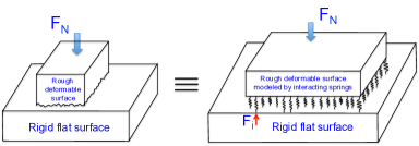
Figure 1: Contact of a rigid flat surface and a rough deformable one with the deformable surface modeled using a set of interacting springs. The only degree of freedom of the springs is normal to the interface.

Constitutive equations relate the deformations and forces of these springs. We prescribe that each spring in contact can sustain a maximum tensile force $F_{th}$. If the force on the spring exceeds $F_{th}$, it snaps out of contact and the force becomes zero. The governing equations are:

$$u_{i}=C_{ij}F_{j},\quad F_{i}\leq F_{th},\quad x_{i}\leq d,$$ (1)

where $u_{i}$ is the length change of the spring ‘i’, $F_{j}$ is the force on spring ‘j’, $C_{ij}$ is the compliance that captures the effect of the force at ‘j’ on an element at ‘i’, $F_{th}$ is the threshold force, $x_{i}=x^{0}_{i}+u_{i}$ is the length of the spring ‘i’ with undeformed length $x^{0}_{i}$, and dilatation $d$ is the distance between the two surfaces. The third expression in (1) is a kinematic constraint corresponding to the rigidity of the flat surface. The undeformed lengths $x^{0}_{i}$ can be used to approximate a desired surface geometry. The compliance $C_{ij}$ is derived from the superposition of the Boussinesq solution for a point force in a semi-infinite half space [8],

$$C_{ij}=\begin{cases}\frac{1-\nu}{2\pi G}\frac{1}{r_{ij}}&i\neq j,\\ \frac{1-\nu}{2\pi G}\frac{3.8}{\Delta}&i=j,\end{cases}$$ (2)

where $\nu,G$ are the Poisson’s ratio and shear modulus of the material, and $r_{ij}$ is the distance between springs ‘i’ and ‘j’, and $\Delta$ is the distance between two neighboring springs. $1/r_{ij}$ becomes singular at $i=j$ since $r_{ij}=0$. This singularity is regularized by assuming that $F_{i}$ is uniformly distributed over a square area with side $\Delta$. The displacements caused by such a pressure distribution was derived by Love [9]. This solution is very close to the Boussinesq solution even for neighboring springs but it is not singular for $i=j$. The case $i=j$ in Equation (2) means that a force at spring ‘i’ deforms it 3.8 times more than a neighboring one. Thus, in computing $u_{i}$ due to $F_{j}$, we use the Boussinesq solution for all $i\neq j$ and the Love solution for $i=j$. A brute-force computation of the $1/r_{ij}$ kernel becomes expensive for large systems. We use the Fast Multipole Method [10] to do this calculation faster. Similar models have been used to study contact, for example see [11] and references therein. Our contribution is the extension to adhesion.

Nondimensionalizing (1) and (2) using $L^{*}$ for length and $F^{*}$ for force, we get:

$$\bar{u}_{i}=\bar{C}_{ij}\bar{F}_{j},\quad\bar{F}_{i}\leq\bar{F}_{th},\quad\bar{x}_{i}\leq\bar{d}.$$ (3)

Setting $F^{*}=2\pi G{L^{*}}^{2}/(1-\nu)$,

$$\bar{C}_{ij}=\begin{cases}1/\bar{r}_{ij}&i\neq j,\\ 3.8/\bar{\Delta}&i=j.\end{cases}$$ (4)

2.1 Algorithm

The forces and the deformations of the springs are coupled through the elastic interactions. Thus, when a spring snaps out of contact, it changes the forces and deformations of neighboring and distant springs (which might then exceed their threshold force). Here, we describe the algorithm we use to simulate displacement-controlled (prescribed dilatation) loading/unloading of the surface.

Given current state $\bar{u}_{i}(\bar{t}),\bar{F}_{i}(\bar{t}),\bar{d}(\bar{t})$ and the set of springs in contact $\mathcal{I}_{c}$

repeat Take a time step $\bar{t}\to\bar{t}+\Delta\bar{t},\bar{d}^{\text{new}}\to\bar{d}+\Delta\bar{d}$

       repeat

             1. for $i=1,\dots,N$ do

                   if $i\in\mathcal{I}_{c}$, set $\bar{u}_{i}=\bar{d}^{\text{new}}-\bar{x}^{0}_{i}$; else, set $\bar{F}_{i}=0$

                  

            compute $\bar{F}_{i}$ for $i\in\mathcal{I}_{c}$ and $\bar{u}_{i}$ for $i\notin\mathcal{I}_{c}$ using the equation in (3) and Equation (4).

             2. for $i=1,\dots,N$ do

                   if $\bar{F}_{i}>\bar{F}_{th}$, set $\bar{F}_{i}=0$, remove $i$ from $\mathcal{I}_{c}$

                   if $\bar{x}^{0}_{i}+\bar{u}_{i}>\bar{d}^{\text{new}}$, add $i$ to $\mathcal{I}_{c}$

                   if one or both of above is true, go back to Step 1.

            

      until All conditions in (3) are met;

until $\bar{t}=\bar{T}$;

Algorithm 1 Algorithm to simulate evolution of the spring system for displacement-controlled loading/unloading.

2.2 Validation using Hertzian contact

To validate our formulation, we simulate Hertzian contact of a linear-elastic sphere of radius $1$ against a rigid flat surface. The two surfaces are initially apart, and the forces and deformations of all the springs are zero. We then decrease the dilatation and compute the evolution of the forces and deformations of the springs using the algorithm described above. The total macroscopic force is obtained as the sum of the spring forces. Compressive values of the force are shown as positive.

The model shows a surprisingly good match with the analytical solution (Figure 2). The elastic constants used in the analytical and numerical solutions are the same and no other parameters have been used in obtaining the numerical results.

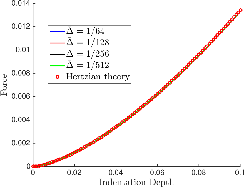
(a)

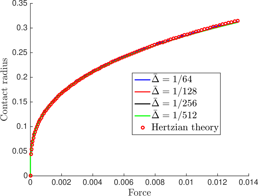
(b)

Figure 2: Comparison of analytical and numerical solutions (at different discretizations) for contact of a linear-elastic sphere against a rigid flat surface (a) indentation depth vs force, (b) force vs contact radius. The model shows a good match with the analytical results.

3 Adhesive contact

Let us now move to the adhesive contact of a sphere. The two surfaces are initially apart and the forces and deformations of all the springs are zero. We then do a displacement-controlled loading-unloading test. We first compress the two surfaces into contact (loading) and then pull them apart (unloading). The parameters used in this simulation are: radius of sphere = 1, $\bar{\Delta}=1/128,\bar{F}_{th}=2\times 10^{-5}$.

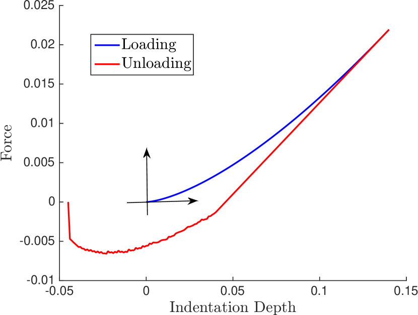
(a)

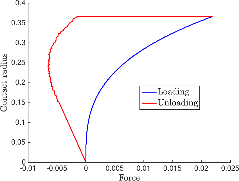
(b)

Figure 3: Loading-unloading test of an adhesive sphere against a rigid flat surface, variation of (a) force with indentation depth and (b) contact radius with force. Since the springs can sustain tension up to a threshold force, the force during unloading is different from that during loading. As we start pulling the surfaces apart, the force becomes tensile, the springs start breaking contact (wiggles in the curves), the force goes through a tensile maximum and eventually drops to zero. During unloading, the area initially remains constant and then starts decreasing as the springs snap off. The force and area drop to zero from a finite nonzero value as observed in some experiments [3].

The loading-unloading behavior is shown in Figure 3. During the loading phase (shown in blue), all springs are in compression and the system is exactly the same as in Hertzian contact. However, the unloading behavior (shown in red) is different and more interesting. Some of the springs are now in tension and thus at the same indentation depth, the total force is different from that during loading. The unloading curve is always lower (force more tensile) than the loading curve. As the surfaces are pulled apart, the springs that reach their threshold force break out of contact. This can be seen as wiggles in the unloading part of the curve (and they are present only in the unloading phase). Upon continued unloading, the total force reaches a tensile maximum. Since we are performing a displacement-controlled simulation, upon further unloading, the tensile force decreases from the maximum and drops to $0$ as all springs snap off (Figure 3(a)). If we did a force-controlled test, the entire contact would break and the force drop to zero at the maximum tensile force. During unloading, before the first spring breaks contact, the contact area remains constant even as the force becomes tensile (Figure 3(b)). As the springs start snapping, the area gradually decreases and goes to zero. Observe that in the final step, both force and contact area drop to zero from a finite nonzero value. This has been observed in experiments as well [3].

3.1 Macroscopic behavior is discretization dependent

Let us study how the numerical solution behaves as we discretize the sphere with more and more springs. We repeat the above simulations with $\bar{\Delta}=1/64,1/128,1/256$ (radius of sphere = 1, $\bar{F}_{th}=2\times 10^{-5}$). The response in the loading phase is the same as that in Hertzian contact (Section 2.2). During unloading, the behavior turns out to be discretization dependent (Figure 4). The maximum tensile force increases with decreasing $\bar{\Delta}$ (Figure 4(a)). The existence of dependence on discretization only during unloading suggests that $\bar{F}_{th}$ cannot be independent of the discretization size; it must decrease with decreasing $\bar{\Delta}$ for convergent macroscopic behavior. The question is, how should $\bar{F}_{th}$ vary with $\bar{\Delta}$?

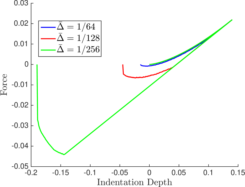
(a)

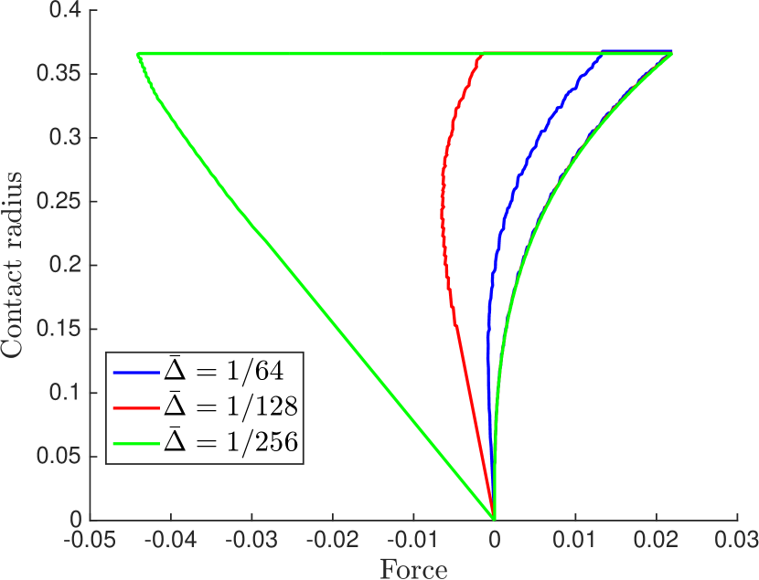
(b)

Figure 4: For the same threshold force, the unloading response depends on the discretization size. The results suggest that the threshold force must decrease with decreasing $\bar{\Delta}$ but what is the right dependence for convergent macroscopic behavior?

3.2 A scaling suggestive of Linear Elastic Fracture Mechanics (LEFM)

For the dependence of threshold force on the discretization size, we consider scalings of the form

$$\bar{F}_{th}=\bar{K}_{th}A^{\alpha},$$ (5)

where $A=\bar{\Delta}^{2}$ is the area of the contact represented by one spring, and $\bar{K}_{th}$ is a constant. Numerical experiments suggest that, for $\alpha=0.75$, the macroscopic behavior converges with decreasing $\bar{\Delta}$ (Figure 5).

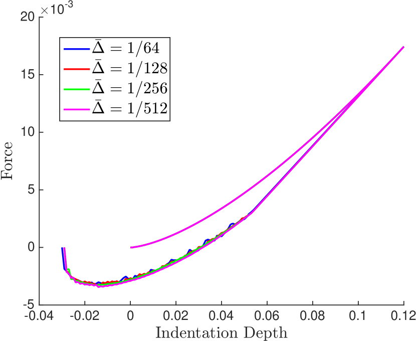
(a)

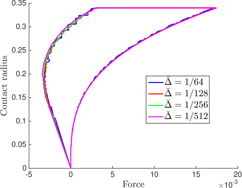
(b)

Figure 5: If the threshold force is scaled as $\bar{F}_{th}=\bar{K}_{th}A^{0.75}$ where $A=\bar{\Delta}^{2}$, the macroscopic behavior becomes independent of $\bar{\Delta}$ (in the above simulations, radius of sphere = 1, $\bar{K}_{th}=2\times 10^{-2}$). This scaling turns out to be analogous to the scaling of the critical stress near a crack tip in Linear Elastic Fracture Mechanics!

This appears puzzling at first, but a little calculation reveals an interesting connection with LEFM. The threshold force scales as

$$\bar{F}_{th}=\bar{K}_{th}A^{0.75}\implies\sigma_{th}=\bar{F}_{th}/A=\bar{K}_{th}A^{-0.25}$$ (6)

where $\sigma_{th}$ is the threshold stress. Using $A=\bar{\Delta}^{2}$,

$$\sigma_{th}=\frac{K_{th}}{\sqrt{\bar{\Delta}}}.$$ (7)

This scaling is suggestive of LEFM. There, the stress at the crack tip is given by (for mode I):

$$\sigma\propto\frac{K_{I}}{\sqrt{r}},$$ (8)

where $K_{I}$ is the mode I stress intensity factor and $r$ is the distance from the crack tip. The criterion for crack propagation is that the stress intensity factor at the crack tip should equal the critical stress intensity factor ($K_{IC}$),

$$K_{I}=K_{IC}\implies\sigma_{C}\propto\frac{K_{IC}}{\sqrt{r}},$$ (9)

where $\sigma_{C}$ is the critical stress (singular at the crack tip). Comparing equations (7) and (9), it is evident that, with $\alpha=0.75$, we have a scaling similar to LEFM with $\bar{K}_{th}$ serving the role of $K_{IC}$. Adhesive contact can be seen from the perspective of fracture mechanics with the area not in contact interpreted as an external crack [7]. This also explains the discretization-size dependence we saw in Figure 4. Without the $\alpha=0.75$ scaling (there $\alpha=0$), by changing $\bar{\Delta}$, we effectively changed $\bar{K}_{th}$ (or $K_{IC}$).

To further bolster this connection between the scaling (Equation (7)) and LEFM, we performed two kinds of tests. First, we did simulations with various other geometries and in each case found that the macroscopic response is discretization-size independent for $\alpha=0.75$ and dependent for $\alpha\neq 0.75$. Further, in our model, the elasticity is captured in the kernel $1/\bar{r}_{ij}$. If the scaling is related to LEFM, it must depend on this kernel. Simulations with other kernels, for example with only local interaction ($\bar{C}_{ij}=C_{0}\delta_{ij}$) or with only a few nearest-neighbor interactions, show that the scaling indeed depends on the kernel. When $\bar{C}_{ij}=C_{0}\delta_{ij}$, i.e., when there is no elastic interaction, the macroscopic response is $\bar{\Delta}$-dependent for $\alpha=0.75$ and independent for $\alpha=1$.

4 Can the model reproduce the JKR results?

Our model is JKR-like since the tensile forces act only within the contact area (as opposed to the DMT model where tensile forces act even outside the contact). Further, the JKR model can also be seen from the perspective of LEFM [7]. Let us further compare the two models. In the JKR model, the maximum tensile force $F_{\text{max}}$ is given by

$$F_{\text{max}}=\frac{3}{2}\pi\gamma R$$ (10)

where $\gamma$ is the fracture energy and $R$ is the radius of the sphere. The maximum force is linear in both the fracture energy and the radius. Let us check these scalings in our model.

We saw that in our model, $\bar{K}_{th}$ is like the critical stress intensity factor $K_{IC}$ in fracture mechanics (Equations (7) and (9)). In LEFM, the critical energy release rate for mode I is $G_{IC}\propto K_{IC}^{2}$. If this is the fracture energy $\gamma$, from Equation (10), and if the same scaling is to hold in our model, the maximum tensile force $\bar{F}_{\text{max}}$ must scale as $\bar{K}_{th}^{2}$. To check this, we repeated the simulations described earlier, increasing $\bar{K}_{th}$ from 0 to 0.04 in steps of 0.01 (radius of sphere = 1, $\bar{\Delta}=1/256$). We find that $\bar{F}_{\text{max}}$ does scale as $(\bar{K}_{th})^{2}$ (Figure 6(a)).

Further, $\bar{F}_{\text{max}}$ must increase linearly with the radius (Equation (10)). This is verified in Figure 6(b) where we show how the maximum tension varies with radius $(\bar{K}_{th}=0.04,\bar{\Delta}=1/256)$.

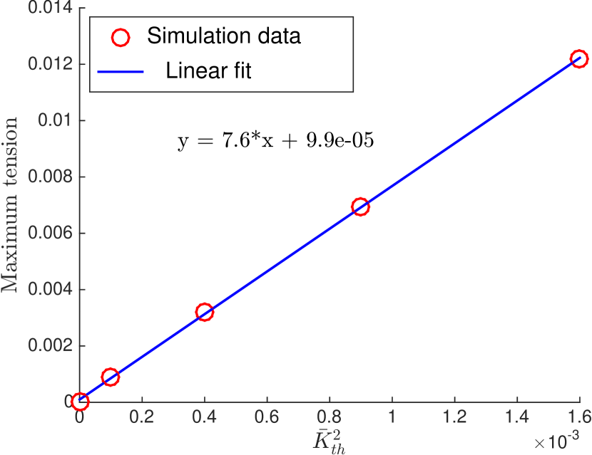
(a)

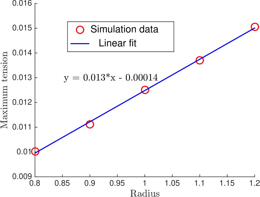
(b)

Figure 6: Scaling of the maximum tensile force with the (a) square of the parameter $\bar{K}_{th}$ and (b) radius. These scalings are the same as in the JKR model.

Our numerical experiments indicate that (Figure 6):

$$\bar{F}_{\text{max}}=7.6\bar{K}_{th}^{2}\bar{R}\implies F_{\text{max}}=\frac{7.6(1-\nu)}{2\pi G}K_{th}^{2}R$$ (11)

where $K_{th}$ has units of MPa $\sqrt{m}$, the same as that of $K_{IC}$ (see the nondimensionalization discussion). From equations 10 and 11,

$$\frac{7.6(1-\nu)}{2\pi G}K_{th}^{2}=\frac{3\pi\gamma}{2}\implies K_{th}=\pi\sqrt{\frac{3G\gamma}{7.6(1-\nu)}}.$$ (12)

This gives the threshold-force parameter $K_{th}$ in our model in terms of the fracture energy $\gamma$ and elastic properties $G,\nu$. Note that $K_{th}$ is a material property independent of the geometry. If $\gamma,G,\nu$ of a material are known, $K_{th}$ can be determined using Equation (12) and used in simulations for any surface geometry.

5 Conclusion

In a system of discrete springs, we study a threshold-force based model for adhesive contact and mode I fracture. Using a scaling of the threshold force with discretization size, we demonstrate the analogy between our model, fracture mechanics, and the JKR adhesion model. The advantage of the model presented here is that it is conceptually simple and easy to implement numerically. Possible applications of the model include studying rough-surface adhesion with long-range elastic interactions and calculation of stress intensity factors for various geometries for mode I fracture. Extension to modes II and III might be possible by adding horizontal degrees of freedom to the springs and using an appropriate kernel based on elasticity solutions. Time-dependent behavior such as viscoelasticity can be incorporated by making the interaction kernel time-dependent ($C_{ij}(t)$) based on solutions of a viscoelastic half-space boundary value problem. In this case, some of the elastic energy stored will be lost by viscoelastic dissipation and interesting rate effects might emerge.

References

- [1] Roya Maboudian and Roger T Howe. Critical review: adhesion in surface micromechanical structures. Journal of Vacuum Science & Technology B, 15(1):1–20, 1997.
- [2] AK Geim, SV Dubonos, IV Grigorieva, KS Novoselov, AA Zhukov, and S Yu Shapoval. Microfabricated adhesive mimicking gecko foot-hair. Nature materials, 2(7):461–463, 2003.
- [3] KL Johnson, K Kendall, and AD Roberts. Surface energy and the contact of elastic solids. Proceedings of the Royal Society of London. A. Mathematical and Physical Sciences, 324(1558):301–313, 1971.
- [4] KNG Fuller and DFRS Tabor. The effect of surface roughness on the adhesion of elastic solids. In Proceedings of the Royal Society of London A: Mathematical, Physical and Engineering Sciences, volume 345, pages 327–342. The Royal Society, 1975.
- [5] R.G Horn, J.N Israelachvili, and F Pribac. Measurement of the deformation and adhesion of solids in contact. Journal of Colloid and Interface Science, 115(2):480–492, February 1987.
- [6] Yeh-Shiu Chu, Sylvie Dufour, Jean Paul Thiery, Eric Perez, and Frederic Pincet. Johnson-Kendall-Roberts Theory Applied to Living Cells. Physical Review Letters, 94(2):028102, January 2005.
- [7] Daniel Maugis. Adhesion of spheres: the JKR-DMT transition using a Dugdale model. Journal of Colloid and Interface Science, 150(1):243–269, 1992.
- [8] Kenneth Langstreth Johnson and Kenneth Langstreth Johnson. Contact mechanics. Cambridge university press, 1987.
- [9] Augustus Edward Hough Love. The stress produced in a semi-infinite solid by pressure on part of the boundary. Philosophical Transactions of the Royal Society of London. Series A, Containing Papers of a Mathematical or Physical Character, pages 377–420, 1929.
- [10] Leslie Greengard and Vladimir Rokhlin. A fast algorithm for particle simulations. Journal of computational physics, 73(2):325–348, 1987.
- [11] Can K Bora, Michael E Plesha, and Robert W Carpick. A numerical contact model based on real surface topography. Tribology Letters, 50(3):331–347, 2013.