Onion-peeling Inversion of Stellarator Images

Abstract

An onion-peeling technique is developed for inferring the emissivity profile of a stellarator plasma from a two-dimensional image acquired through a CCD or CMOS camera. Each pixel in the image is treated as an integral of emission along a particular line-of-sight. Additionally, the flux surfaces in the plasma are partitioned into discrete layers, each of which is assumed to have uniform emissivity. If the topology of the flux surfaces is known, this construction permits the development of a system of linear equations that can be solved for the emissivity of each layer. We present initial results of this method applied to wide-angle visible images of the CNT stellarator plasma.

I Introduction

A number of well-established techniques exist for inferring plasma emission profiles based on line-of-sight measurements. The measurements are interpreted as line integrals of emission and are typically acquired in 1D or 2D arrays. This poses a question of “inverting” the acquired datasets into 2D or 3D maps, respectively, of plasma emissivity of the particle or wavelength of interest.

Tomography has succeeded at this in tokamaks Ingesson et al. (2008) and stellarators Sallander et al. (2000), primarily for X-ray and visible emission Gota et al. (2006); Asai et al. (2006). Tomography does not require knowledge of the flux surface geometry, although the geometry can constrain the tomography for better results. A disadvantage, though, is that it requires several cameras around the plasma.

Under the assumption of the flux surface geometry being perfectly known, a single camera is sufficient. If, additionally, the flux surfaces are axisymmetric, one can use the Abel transform Abel (1826); Dasch (1992). This is appropriate in quiescent tokamak and spherical tokamak plasmas.

In stellarators it is reasonable to assume a good knowledge of the flux surfaces, which are nearly entirely determined by external currents and are magnetohydrodynamically more quiescent than in tokamaks and sperical tokamaks. This is especially true when the ratio of kinetic pressure to magnetic pressure, $\beta$, is low: in that case, stellarator equilibria are easier to compute, faithful to experiments and magnetohydrodynamically stable. However, stellarator flux-surfaces are obviously not axisymmetric.

The onion peeling algorithm Dasch (1992) can be considered a generalization of the Abel inversion to non-axisymmetric problems. Onion peeling is used here to invert wide-angle visible images of a stellarator plasma for the first time. The work was performed at the CNT stellarator Pedersen et al. (2004) and takes advantage of a recent experimental and numerical study of its field errors Hammond et al. (2016), giving good confidence in the knowledge of its flux surfaces. The method is described in Sec.II. Sec.III is devoted to the “forward problem”: toy models of the emissivity profile are translated in the corresponding images expected to be acquired by the camera. The synthetic image corresponding to an edge-peaked profile is in best qualitative agreement with the actual experimental images. The inverse problem is solved in Sec.IV. The method is first tested with a glow discharge plasma for validation and then applied to a microwave-heated plasma.

II Method

The method used in this paper for reconstructing the emissivity profile relies on two principal assumptions. The first is that the plasma can be modeled as a set of nested discrete layers, each of which has a uniform emissivity. In the context of a toroidal magnetic confinement device, these layers are bounded by flux surfaces (Fig. 1). The second assumption is that the emissive layers contribute to the brightness of each camera pixel in proportion to the distance that the pixel’s line-of-sight travels through each layer.

With these assumptions in place, the brightness $p$ of each pixel is related to the emissivity of each layer by a system of linear equations,

$$b\mathbf{p}=L\mathbf{e},$$ (1)

where $p_{i}$ is brightness of the $i^{th}$ pixel, $b$ is a constant of proportionality, $L_{ij}$ is the total distance traveled by the $i^{th}$ pixel’s line-of-sight throught the $j^{th}$ layer, and $e_{j}$ is the emissivity of the $j^{th}$ layer. The elements of the matrix $L$ can be calculated based on knowledge of (1) the flux surfaces, (2) the camera’s position, orientation, and field of view, and (3) the positions of any obstacles (such as CNT’s in-vessel coils) obstructing the camera’s view of portions of the plasma. For the low-$\beta$ plasmas studied in CNT for this work, any differences from the measured vacuum flux surfaces were neglected.

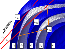
Figure 1: Schematic illustration of the onion-peeling method. The red lines represent lines-of-sight of two camera pixels whose brightness is denoted by $p_{1}$ and $p_{2}$. The lines-of-sight both travel through one or more layers of plasma, whose borders are shown as alternating blue and white surfaces. The lengths of the segments within the respective surfaces constitute the components of the $L$ matrix as defined in the text. Note that some components (like $L_{21}$ here) are actually due to the sum of two or more segments due to multiple crossings of a layer. The terms $e_{i}$ are the emissivities of each layer.

The pixel data tends to be noisy and can exhibit nontrivial correlations. Hence, if one is to reconstruct the emissivity profile based on pixel data, it is best to have many more pixels than layers to reconstruct. An unbiased estimator of the emissivity profile can then be expressed asJones and Finn (2006)

$$\mathbf{e}\approx\left(L^{T}C^{-1}L\right)^{-1}L^{T}C^{-1}~{}b\mathbf{p},$$ (2)

where $C$ is the covariance matrix for the pixel noise.

When the emissivity profile $\mathbf{e}$ is calculated in this way, it is informative to plug it back into Eq. 1 to synthesize an image $\mathbf{p}^{*}$ for comparison with the original image.

III Forward problem

As an initial proof-of-concept and a test of the reliability of the calculations of $L$, synthetic images were generated based on profiles that were specified a priori. $L$ was calculated to correspond to a camera view similar to that of the photograph shown in Fig. 2. The test profiles were given three basic functional forms: hollow (linearly increasing from core to edge), uniform, and peaked (linearly decreasing from core to edge).

These profiles and the resulting synthetic images are shown in Fig. 3. Of the three test profiles, the hollow one (Fig. 3b) has the best qualitative agreement with the photograph in Fig. 2, suggesting that the plasma in the photo (which is typical of the $\approx 1kW$ electron cyclotron resonant heating (ECRH) discharges studied in CNT) has greater visible emission at the edge than in the core. This is consistent with a higher rate of recombination reactions occurring in the colder edge.

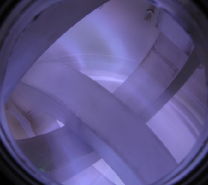
Figure 2: Photograph of a typical argon plasma in CNT heated with 1 kW ECRH with CNT’s two in-vessel coils in clear view.

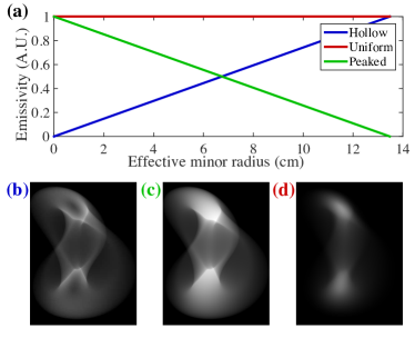
Figure 3: Simulated images of three synthetic profiles. (a) profiles; (b) image of hollow profile; (c) image of uniform profile; (d) image of peaked profile. The upper halves of of (b)-(d) approximate the field of view of the photo in Fig. 2.

IV Inversion of experimental images

IV.1 Image processing

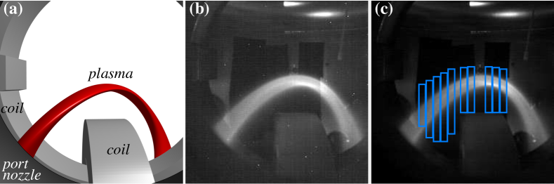
Figure 4: (a) Schematic of the key objects in the camera’s field of view. (b) Raw image of a typical glow discharge (Sect. IV.2). (c) The same image, after noise subtraction, with boxes indicating the regions where pixel data were used for reconstructions (Sect. IV.1).

Images used for profile reconstructions were acquired by a high-speed CMOS camera manufactured by Canadian Photonics. The camera was placed outside the vacuum chamber with a view through a fused silica window. The field of view is shown in Fig. 4. As Eq. 1 does not account for external sources of light, sheets of low-outgassing black foil manufactured by Acktar were fixed to the internal vessel walls to prevent reflection in the camera’s lines-of-sight.

To account for pixel noise, a large number of frames (greater than or equal to the total number of pixels to be analyzed) was acquired with no light sources present. The mean value of the noise acquired for each pixel was then subtracted from the corresponding pixel in a plasma image. The result of this subtraction is shown in Fig. 4b. The background frames were also used to compute the pixel noise covariance matrix $C$ for the inversion (Eq. 2). Optical noise originating from the chamber was neglected. The propagated error $\sigma_{\text{noise},j}$ for the $j^{th}$ layer in the profile was calculated as the square root of the $j^{th}$ diagonal element of the posterior covariance matrixJones and Finn (2006), given by $\left(L^{T}C^{-1}L\right)^{-1}$.

For each plasma image, ten independent inversions were conducted using disjoint subsets of the pixels (shown as blue boxes in Fig. 4b). The subsets used in this work contained between 560 and 860 pixels. To be included in a subset, a pixel’s line-of-sight needed to terminate against black foil. The ten different profiles $\mathbf{e}$ obtained from each of the subsets were then averaged to obtain a final reconstructed profile. This was done to partially cancel the effects of small errors in the camera alignment, which would otherwise cause some contributions to some pixels to be misattributed to layers not within their lines-of-sight. The standard deviation among these measurements will be notated as $\sigma_{\text{align}}$.

The total uncertainty of the emission from the $j^{th}$ layer was then computed from the quadrature sum of the alignment error $\sigma_{\text{align}}$ and the noise error $\sigma_{\text{noise}}$ averaged over $N$ pixel subsets:

$$\sigma_{j}=\sqrt{\frac{{\sigma_{\text{align},j}}^{2}}{N}+\left(\sum_{n}^{N}\frac{{\sigma_{\text{noise},nj}}}{N}\right)^{2}}$$ (3)

IV.2 Reconstructions of glow discharges

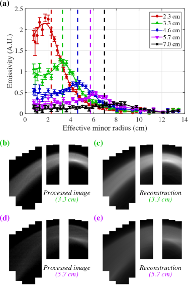
Figure 5: Reconstructed profiles and images of glow discharges. (a) Profiles with the emissive filament located on six different flux surfaces with effective minor radii given in the legend and as vertical dashed lines. Solid curves are fits to cubic smoothing splines, which are used for the image reconstructions. (b)-(c) Image and reconstruction for the 3.3 cm filament position in the regions where pixel data were used for reconstructions (Fig. 4b). (d)-(e) Image and reconstruction for the 5.7 cm filament position.

Field line and flux surface visualizations are often utilized in CNT for diagnostic alignment. Brenner et al. (2008) These are discharges maintained by a heated, biased filament. They tend to emit a visible glow that is localized to the flux surface where the filament is located. In the case of rational or near-rational surfaces, the glow is restricted to the flux tube connecting one side of the filament to the other. On non-rational surfaces, however, the entire surface tends to be emissive.

While this glow is not perfectly uniform, it is nonetheless expected that an inversion of such a glow would result in an emission profile that is peaked around the layer where the emitter is located. Hence, inversions of glow discharges can serve as tests of the method’s validity.

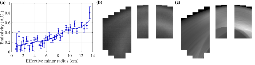
Figure 6: Reconstruction of a 1 kW ECRH discharge. (a) Emissivity profile with a cubic spline fit. (b) Photographic data used for the reconstruction. (c) Synthesized image based on the reconstructed profile.

Quiescent glow discharges were filmed at 25 frames per second with 15 ms exposures at the camera’s lowest gain setting. Fig. 5a shows emissivity profiles from glow discharges from several filament locations at successively larger effective minor radii. As expected, each profile is peaked. Additionally, the peak locations agree well with the locations of the filament, which were measured independently through field line mapping procedures similar to those described in Refs. Pedersen et al. (2006); Jaenicke et al. (1993). Glow discharges on surfaces with larger minor radii tend to have lower calculated emissivity overall; this is consistent with visual inspection of the discharges.

Fig. 5b-e show raw and reconstructed images corresponding to two of the profiles from Fig. 5a. While the agreement is qualitatively good in many respects, there are some features from the photos that are not replicated in the reconstructions. Perhaps the most noticeable are the bright, narrow streaks that are visible in the middle of the plasmas in the center and left of Figs. 5b,d. The streak is a nonuniformity on its surface (even on non-rational surfaces, regions with short connection lengths to the filament tend to glow brigher than the rest of the surface). Such a nonuniformity is not expected to carry over in the inversion process, due to the assumption of uniform emissivity within a layer discussed in Sec. II.

IV.3 Reconstruction of an ECRH discharge

1 kW ECRH discharges lasting for roughly 7 ms were filmed at 500 frames per second with 2 ms exposures at the lowest gain setting. Fig. 6 shows a profile, image data, and reconstructed image from a typical frame. Note that, except for the outermost layer, the profile follows a roughly linear trend similar to the hollow test profile in Fig. 3. In contrast to the image comparisons from Fig. 5, in which the image data had fine structure that did not appear in the reconstructions, the reconstruction for the ECRH discharge in Fig. 6c has fine structure that is not visible in the image data (Fig. 6b). Much of the structure in the reconstruction results from the jump in emissivity at the edge as seen in the profile, which would result in bright spots wherever the outermost layer is nearly tangent to lines-of-sight. It is not fully understood why the jump in emissivity appears in the calculated profile despite not appearing experimentally. It is conjectured that it may be a spurious effect resulting from emission outside the closed flux surfaces; i.e., in the scrape-off layer.

V Summary, Conclusions and Future work

In summary, a method has been implemented for deducing the emissivity profile of a nonaxisymmetric toroidal plasma based on images from a single camera location. Reconstructions of flux surface visualizations yielded peaked profiles as expected, thereby serving as a promising test of concept. The fact that the non-uniform features from the photographs of the glow discharges did not appear in the reconstructed images serves to emphasize that this method will not account for non-uniformities in emission across a layer. A reconstruction of an ECRH discharge contained some unexpected features but still exhibited an overall hollow profile, consistent with expectations.

Future work will include incorporating the scrape-off layer in the onion-peeling inversion. A further improvement would be to cover larger portions of the CNT vessel, as well as the interlocked coils, with the light-absorbing material. As a result, larger portions of the experimental images would be suitable for inversion.

The technique will then be deployed to study the variation of the emissivity profile over the course of ECRH heating pulses. Profiles will be compared under different magnetic configurations and heating locations. Optical filters may also be placed in front of the camera lens to isolate particular emission lines.