Theoretical estimate on tensor-polarization asymmetry
in proton-deuteron Drell-Yan process

Abstract

Tensor-polarized parton distribution functions are new quantities in spin-one hadrons such as the deuteron, and they could probe new quark-gluon dynamics in hadron and nuclear physics. In charged-lepton deep inelastic scattering (DIS), they are studied by the twist-two structure functions $b_{1}$ and $b_{2}$. The HERMES collaboration found unexpectedly large $b_{1}$ values than a naive theoretical expectation based on the standard deuteron model. The situation should be significantly improved in the near future by an approved experiment to measure $b_{1}$ at JLab (Thomas Jefferson National Accelerator Facility). There is also an interesting indication in the HERMES result that finite antiquark tensor polarization exists. It could play an important role in solving a mechanism on tensor structure in the quark-gluon level. The tensor-polarized antiquark distributions are not easily determined from the charged-lepton DIS; however, they can be measured in a proton-deuteron Drell-Yan process with a tensor-polarized deuteron target. In this article, we estimate the tensor-polarization asymmetry for a possible Fermilab Main-Injector experiment by using optimum tensor-polarized PDFs to explain the HERMES measurement. We find that the asymmetry is typically a few percent. If it is measured, it could probe new hadron physics, and such studies could create an interesting field of high-energy spin physics. In addition, we find that a significant tensor-polarized gluon distribution should exist due to $Q^{2}$ evolution, even if it were zero at a low $Q^{2}$ scale. The tensor-polarized gluon distribution has never been observed, so that it is an interesting future project.

I Introduction

It was discovered by the European Muon Collaboration (EMC) collaboration in the measurement of the polarized structure function $g_{1}$ that only a small fraction of nucleon spin is carried by quarks nucleon-spin , which is in contradiction to the naive quark model. Since then, many theoretical and experimental efforts have been made to clarify the origin of the nucleon spin. There could be contributions from gluon spin and partonic angular momenta. Theoretical and experimental efforts are in progress to solve the issue.

On the other hand, there are new polarized structure functions fs83 ; hjm89 , which do not exist in the spin-1/2 nucleon, for spin-one hadrons and nuclei such as the deuteron. In charged-lepton deep inelastic scattering, they are named as $b_{1}$, $b_{2}$, $b_{3}$, and $b_{4}$ hjm89 . Projection operators of $b_{1-4}$ on the hadron tensor $W_{\mu\nu}$ are obtained in Ref. kk08 . The twist-two functions are $b_{1}$ and $b_{2}$, and they are related with each other by the Callan-Gross like relation $2xb_{1}=b_{2}$ in the Bjorken scaling limit. Therefore, it is interesting to investigate the leading-twist one $b_{1}$ (or $b_{2}$) first. A useful sum rule for the twist-two function $b_{1}$ was proposed in Ref. b1-sum by using the parton model, and it could be used as a guideline for the existence of tensor-polarized antiquark distributions. On the other hand, proton-deuteron Drell-Yan processes are theoretically formulated in Ref. pd-drell-yan for the polarized deuteron including tensor polarization.

The leading-twist structure function $b_{1}$ probes a peculiar aspect of internal structure in a spin-one hadron. It vanishes if internal constituents are in the S wave, which indicates that it is a suitable observable for probing a dynamical aspect, possibly an exotic one, inside the hadron. In fact, the first measurement of $b_{1}$ by the HERMES collaboration hermes05 indicated that the magnitude of $b_{1}$ is much larger than the one expected by the standard deuteron model with D-state admixture hjm89 ; kh91 . There could be other effects from pions miller-b1 and shadowing phenomena b1-shadowing in the deuteron. There is also a suggestion that $b_{1}$ studies could lead to a new finding on a hidden-color component miller-b1 . On related spin-one hadron physics, there are investigations on leptoproduction of spin-one hadron rho-production , fragmentation functions spin-1-frag , generalized parton distributions spin-1-gpd , target-mass corrections mass-corr , positivity constraints dmitrasinovic-96 , lattice QCD estimate lattice , and angular momenta for spin-1 hadron angular-spin-1 .

The first measurement of $b_{1}$ was done by the HERMES collaboration in 2005 hermes05 . Its data indicated that $b_{1}$ has interesting oscillatory behavior as the function of $x$ and that the magnitude of $xb_{1}$ is of the order of $10^{-3}$. Since $b_{1}$ is expressed by tensor-polarized parton distribution functions, possible quark and antiquark distributions ($\delta_{T}q(x)$, $\delta_{T}\bar{q}(x)$) were extracted from the HERMES data tensor-pdfs . The analysis suggested finite tensor-polarized antiquark distributions from the data at $x<0.1$. Although the sign change of $b_{1}$ is expected in a convolution description for the deuteron with D-state admixture, the HERMES data indicate much larger $|\,b_{1}|$. Therefore, the $b_{1}$ is expected to probe non-conventional physics beyond the standard deuteron model. The HERMES measurement also suggested a new phenomena on a finite tensor polarization for antiquarks. There is a sum rule for $b_{1}$ b1-sum , and a deviation from this sum indicated the finite tensor-polarized antiquark distributions in the similar way to Gottfried sum-rule violation flavor3 .

The deuteron tensor structure has been investigated for a long time at low energies. However, time has come to investigate it, through the tensor-polarized structure functions and parton distribution functions, in terms of quark and gluon degrees of freedom. Furthermore, these quantities could be sensitive to exotic features such as the hidden color miller-b1 . In the HERMES measurement, there is already a hint that new hadron physics is needed to interpret its data. Therefore, a new field of high-energy spin physics could be created by investigating the tensor structure functions, as the EMC measurement created the field of high-energy spin physics for the spin-1/2 nucleon. The current situation on $b_{1}$ and tensor-polarized PDFs is summarized in Ref. sk14 .

By considering this prominent prospect, the Thomas Jefferson National Accelerator Facility (JLab) experiment was approved for measuring the structure function $b_{1}$ Jlab-b1 , and the actual experiment will start in a few years. In addition, the related tensor polarization $A_{zz}$ can be investigated at JLab in the large-$x$ region azz . These $b_{1}$ and $A_{zz}$ could be also investigated at the future Electron-Ion Collider (EIC) eic .

In a simple model for the deuteron, it is not obvious to have a tensor-polarized antiquark distribution; however, a finite value is indicated in the HERMES experiment for the antiquark tensor polarization. The best way to probe the antiquark distributions is to use a Drell-Yan process with a tensor-polarized deuteron target pd-drell-yan . The Drell-Yan process for unpolarized proton - tensor-polarized deuteron is possible, and its measurement is now under consideration at Fermilab Fermilab-MI . However, there is no theoretical estimate on the tensor-polarized spin asymmetry, so that it is necessary to show even the order of magnitude for an experimental proposal, especially for considering beam-time allocation in an actual measurement. The purpose of this article is to show expected spin asymmetries for the Fermilab measurement.

In this article, we explain formalisms first in Sec. II, especially on the tensor-polarized structure functions and parton distribution functions (PDFs) in Sec. II.1, and the tensor-polarized Drell-Yan spin asymmetry is expressed in terms of the tensor-polarized PDFs in Sec. II.2. Then, our estimates on the spin asymmetry are shown for the possible Fermilab experiment in Sec. III. The results are summarized in Sec. IV.

II Tensor-polarized distribution functions for spin-one deuteron

We explain basic formalisms involving tensor-polarized structure functions and PDFs in deep inelastic charged-lepton scattering and proton-deuteron Drell-Yan process.

II.1 Tensor-polarized structure functions
in charged-lepton deep inelastic scattering

First, the charged-lepton deep inelastic scattering (DIS) from the polarized deuteron is explained. The polarized DIS formalism for the charged-lepton from the nucleon is well known, and it is generally expressed in terms of four structure functions, $F_{1}$, $F_{2}$, $g_{1}$, and $g_{2}$. In addition to these functions, there exist four new structure functions, $b_{1}$, $b_{2}$, $b_{3}$, and $b_{4}$, in the DIS from the spin-one hadron such as the deuteron.

In the charged-lepton DIS shown in Fig. 1, the hadron tensor $W_{\mu\nu}$ is generally expressed for a spin-one hadron as hjm89 ; kk08 ; sk14

$$W_{\mu\nu}^{\lambda_{f}\lambda_{i}}= \frac{1}{4\pi M}\int d^{4}\xi\,e^{iq\cdot\xi}\,\langle\,p,\lambda_{f}\,|\,[\,J_{\mu}^{\,em}(\xi),J_{\nu}^{\,em}(0)]\,|\,p,\lambda_{i}\,\rangle$$

$$= -F_{1}\hat{g}_{\mu\nu}+\frac{F_{2}}{M\nu}\hat{p}_{\mu}\hat{p}_{\nu}+\frac{ig_{1}}{\nu}\epsilon_{\mu\nu\lambda\sigma}q^{\lambda}s^{\sigma}+\frac{ig_{2}}{M\nu^{2}}\epsilon_{\mu\nu\lambda\sigma}q^{\lambda}(p\cdot qs^{\sigma}-s\cdot qp^{\sigma})$$

$$-b_{1}r_{\mu\nu}+\frac{1}{6}b_{2}(s_{\mu\nu}+t_{\mu\nu}+u_{\mu\nu})+\frac{1}{2}b_{3}(s_{\mu\nu}-u_{\mu\nu})+\frac{1}{2}b_{4}(s_{\mu\nu}-t_{\mu\nu}),$$ (1)

by the eight structure functions including the new ones $b_{1-4}$. Here, the kinematical coefficients $r_{\mu\nu}$, $s_{\mu\nu}$, $t_{\mu\nu}$, and $u_{\mu\nu}$ are defined as

$$r_{\mu\nu}= \frac{1}{\nu^{2}}\bigg{[}q\cdot E^{*}(\lambda_{f})q\cdot E(\lambda_{i})-\frac{1}{3}\nu^{2}\kappa\bigg{]}\hat{g}_{\mu\nu},\ \ \ \ s_{\mu\nu}=\frac{2}{\nu^{2}}\bigg{[}q\cdot E^{*}(\lambda_{f})q\cdot E(\lambda_{i})-\frac{1}{3}\nu^{2}\kappa\bigg{]}\frac{\hat{p}_{\mu}\hat{p}_{\nu}}{M\nu},$$

$$t_{\mu\nu}= \frac{1}{2\nu^{2}}\bigg{[}q\cdot E^{*}(\lambda_{f})\left\{\hat{p}_{\mu}\hat{E}_{\nu}(\lambda_{i})+\hat{p}_{\nu}\hat{E}_{\mu}(\lambda_{i})\right\}+\left\{\hat{p}_{\mu}\hat{E}_{\nu}^{*}(\lambda_{f})+\hat{p}_{\nu}\hat{E}_{\mu}^{*}(\lambda_{f})\right\}q\cdot E(\lambda_{i})-\frac{4\nu}{3M}\hat{p}_{\mu}\hat{p}_{\nu}\bigg{]},$$

$$u_{\mu\nu}= \frac{M}{\nu}\bigg{[}\hat{E}_{\mu}^{*}(\lambda_{f})\hat{E}_{\nu}(\lambda_{i})+\hat{E}_{\nu}^{*}(\lambda_{f})\hat{E}_{\mu}(\lambda_{i})+\frac{2}{3}\hat{g}_{\mu\nu}-\frac{2}{3M^{2}}\hat{p}_{\mu}\hat{p}_{\nu}\bigg{]}.$$ (2)

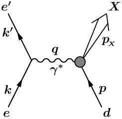
Figure 1: Deep inelastic scattering of charged lepton ($e$) from spin-one hadron $d$.

In these equations, $k$ and $k^{\prime}$ are initial and final lepton momenta, $M$, $p$, and $q$ are hadron mass, hadron momentum, and momentum transfer, $\nu$ and $Q^{2}$ are defined by $\nu={p\cdot q}/{M}$, and $Q^{2}=-q^{2}>0$, $p_{{}_{X}}$ is given by $p_{{}_{X}}=p+q$, and $\epsilon_{\mu\nu\lambda\sigma}$ is an antisymmetric tensor with the convention $\epsilon_{0123}=+1$. The notations $\hat{g}_{\mu\nu}$ and $\hat{p}_{\mu}$ are used for satisfying the current conservation $q^{\mu}W_{\mu\nu}=q^{\nu}W_{\mu\nu}=0$, and they are defined by

$$\hat{g}_{\mu\nu}\equiv g_{\mu\nu}-\frac{q_{\mu}q_{\nu}}{q^{2}},\ \ \hat{a}_{\mu}\equiv a_{\mu}-\frac{a\cdot q}{q^{2}}q_{\mu}.$$ (3)

Furthermore, $\kappa$ is defined by $\kappa=1+{Q^{2}}/{\nu^{2}}$, $s^{\mu}$ is the spin vector of the spin-one hadron, and $E^{\mu}$ is the polarization vector of the spin-one hadron with the constraints, $p\cdot E=0$ and $E^{*}\cdot E=-1$. The polarization vector is taken as the spherical unit vectors:

$$E^{\mu}(\lambda=\pm 1) =\frac{1}{\sqrt{2}}(0,\mp 1,-i,0),$$

$$E^{\mu}(\lambda=0) =(0,0,0,1),$$ (4)

and its relation to the the spin vector is given by

$$(s_{\lambda_{f}\lambda_{i}})^{\mu}=-\frac{i}{M}\epsilon^{\mu\nu\alpha\beta}E^{*}_{\nu}(\lambda_{f})E_{\alpha}(\lambda_{i})p_{\beta}.$$ (5)

In these equations, we explicitly denoted the initial and final spin states by $\lambda_{i}$ and $\lambda_{f}$, respectively, because off-diagonal terms with $\lambda_{f}\neq\lambda_{i}$ are generally needed to discuss higher-twist contributions hjm89 .

Among the four new structure functions $b_{1-4}$, $b_{3}$ and $b_{4}$ are higher-twist functions, and the twist-two functions $b_{1}$ and $b_{2}$ are related with each other by the Callan-Gross like relation $2xb_{1}=b_{2}$ in the Bjorken scaling limit. The functions $b_{1}$ and $b_{2}$ are expressed by the tensor-polarized parton distribution functions $\delta_{T}f(x)$ defined by delta-T-notation

$$\!\!\delta_{{}_{T}}f(x,Q^{2})\equiv f^{0}(x,Q^{2})-\frac{f^{+1}(x,Q^{2})+f^{-1}(x,Q^{2})}{2},$$ (6)

where $f^{\lambda}$ indicates an unpolarized parton distribution in the hadron spin state $\lambda$. Using the tensor-polarized quark and antiquark distributions, we have the structure function

$$b_{1}(x,Q^{2})=\frac{1}{2}\sum_{i}e_{i}^{2}\,\left[\delta_{{}_{T}}q_{i}(x,Q^{2})+\delta_{{}_{T}}\bar{q}_{i}(x,Q^{2})\right],$$ (7)

in the parton model. Here, $e_{i}$ is the charge of the quark flavor $i$.

There is sum rule for $b_{1}$ based on the parton model b1-sum ; tensor-pdfs in the similar way to the Gottfried sum rule flavor3 :

$$\!\!\!\int dx\,b_{1}(x) =-\lim_{t\to 0}\frac{5}{24}\,t\,F_{Q}(t)$$

$$\ \ \ +\frac{1}{9}\int dx\,\left[\,4\,\delta_{{}_{T}}\bar{u}(x)+\delta_{{}_{T}}\bar{d}(x)+\delta_{{}_{T}}\bar{s}(x)\,\right],$$

$$\int\frac{dx}{x}\,[F_{2}^{p} (x)-F_{2}^{n}(x)]=\frac{1}{3}+\frac{2}{3}\int dx\,[\bar{u}(x)-\bar{d}(x)],$$ (8)

where $F_{Q}(t)$ is the electric quadrupole form factor for the spin-one hadron, and this first term vanishes: $\lim_{t\to 0}\frac{5}{24}tF_{Q}(t)=0$. These relations are derived in the parton model, and they are not rigorous ones obtained, for example, by the current algebra ioffe-book . Therefore, depending on small-$x$ behavior of $\bar{u}-\bar{d}$ (or $F_{2}^{p}-F_{2}^{n}$) and $\delta_{T}\bar{q}$ (or $b_{1}$), these sums may diverge although $\bar{u}$ and $\bar{d}$ are currently assumed to be equal at very small $x$ where experimental data do not exist. These sum rules should be considered as guidelines based on the parton model. In any case, as the violation of the Gottfried sum rule created the field of flavor dependence in antiquark distributions and studies of nonperturbative mechanisms behind it, the deviation from zero for the $b_{1}$ sum could probe the interesting tensor-polarized antiquark distributions $\delta_{T}\bar{q}$ and possibly exotic mechanisms behind them as shown in Eq. (8).

The HERMES collaboration reported the first measurement on $b_{1}$ hermes05 , and its data were analyzed to obtain possible tensor-polarized PDFs in Ref. tensor-pdfs . Since there is little information for the tensor-polarized PDFs at this stage, we need to introduce bold assumptions for extracting the distributions from the experimental data. However, the $b_{1}$ seems to have a node at a medium $x$ point. First, a conventional convolution description for $b_{1}$ indicates an oscillatory $x$ dependence hjm89 ; kh91 . Namely, it is negative at $x>0.5$ and it turns into positive at $x<0.5$. Second, the sign change is also suggested by the HERMES data at $x=0.2-0.3$. Third, the $b_{1}$ sum needs the node to satisfy $\int dx\,b_{1}(x)=0$. From these ideas, we considered that tensor-polarized PDFs for the deuteron are expressed by the unpolarized PDFs multiplied by a function $\delta_{{}_{T}}w(x)$ at $Q_{0}^{2}$ as tensor-pdfs

$$\delta_{{}_{T}}q_{v}^{D}(x,Q_{0}^{2}) \equiv\delta_{{}_{T}}u_{v}^{D}(x,Q_{0}^{2})=\delta_{{}_{T}}d_{v}^{D}(x,Q_{0}^{2})$$

$$=\delta_{{}_{T}}w(x)\,\frac{u_{v}(x,Q_{0}^{2})+d_{v}(x,Q_{0}^{2})}{2},$$

$$\delta_{{}_{T}}\bar{q}^{D}(x,Q_{0}^{2}) \equiv\delta_{{}_{T}}\bar{u}^{D}(x,Q_{0}^{2})=\delta_{{}_{T}}\bar{d}^{D}(x,Q_{0}^{2})$$

$$=\delta_{{}_{T}}s^{D}(x,Q_{0}^{2})=\delta_{{}_{T}}\bar{s}^{D}(x,Q_{0}^{2})$$

$$=\alpha_{\bar{q}}\,\delta_{{}_{T}}w(x)\,$$

$$\!\!\!\!\!\!\!\!\!\!\!\!\!\!\!\!\!\!\!\!\!\!\times\frac{2\bar{u}(x,Q_{0}^{2})+2\bar{d}(x,Q_{0}^{2})+s(x,Q_{0}^{2})+\bar{s}(x,Q_{0}^{2})}{6}.$$ (9)

Here, $D$ indicates the deuteron and the capital letter is used to avoid a confusion with a d-quark, and the modification function $\delta_{{}_{T}}w(x)$ is expressed by a simple polynomial form with a node at $x=x_{0}$:

$$\delta_{{}_{T}}w(x)=ax^{b}(1-x)^{c}(x_{0}-x).$$ (10)

It means that a certain fraction of the unpolarized PDFs is tensor-polarized, and this fraction is given by $\delta_{{}_{T}}w(x)$ or $\alpha_{\bar{q}}\,\delta_{{}_{T}}w(x)$ for valence-quark and antiquark distributions, respectively. In the analysis of Ref. tensor-pdfs , the scale is taken as the average $Q^{2}$ of the HERMES experiment ($Q_{0}^{2}=2.5$ GeV²). The parameters $a$, $b$, $c$, and $x_{0}$ are determined by a $\chi^{2}$ analysis of the HERMES data with the leading-order expression for $b_{1}$ in Eq. (7) by considering two options:

• Set 1: There is no tensor-polarized antiquark distribution at the scale $Q_{0}^{2}$ ($\alpha_{\bar{q}}=0$).

• Set 2: There could be finite tensor-polarized antiquark distributions at the scale $Q_{0}^{2}$ ($\alpha_{\bar{q}}$ is a free parameter).

The determined parameter values are $a=0.221\pm 0.174$ ($0.378\pm 0.212$), $b=0.648\pm 0.342$ ($0.706\pm 0.324$), $\alpha_{\bar{q}}=3.20\pm 2.75$ (fixed$=0$), $c=\text{fixed}=1$ ($1$), and $x_{0}=0.221$ (0.229) in the set-2 (set-1).

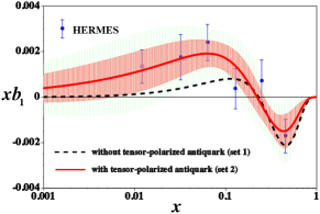
Figure 2: (Color online) $\chi^{2}$ analysis results are compared with HERMES data hermes05 . The solid and dashed curves indicate theoretical results with finite tensor-polarized antiquark distributions (set-2, $\alpha_{\bar{q}}\neq 0$) and without them (set-1, $\alpha_{\bar{q}}=0$), respectively. The open circle is the data at $Q^{2}<1$ GeV², and it is not included in the fit analysis tensor-pdfs . The uncertainties of the set-2 curve are shown by the bands with $\Delta\chi^{2}=1$ and 3.53.

Since the error matrix or Hessian is obtained in the $\chi^{2}$ analysis, it is possible to show an error band for the obtained $b_{1}$ curve. The details of the Hessian method is explained elsewhere hessian , so that a brief outline is explained in the following. Expanding $\chi^{2}$ around the minimum parameter set $\hat{\xi}$, we have the $\chi^{2}$ change ($\Delta\chi^{2}$) expressed by the second derivative matrix $H_{ij}$, which is called Hessian, as

$$\Delta\chi^{2}=\chi^{2}(\hat{\xi}+\delta\xi)-\chi^{2}(\hat{\xi})=\sum_{i,j}H_{ij}\,\delta\xi_{i}\,\delta\xi_{j}.$$ (11)

Then, the error of a physics quantity $f(x)$ is calculated by the Hessian and as

$$[\delta f(x)]^{2}=\Delta\chi^{2}\sum_{i,j}\left[\frac{\partial f(x)}{\partial\xi_{i}}\right]_{\hat{\xi}}H_{ij}^{-1}\left[\frac{\partial f(x)}{\partial\xi_{j}}\right]_{\hat{\xi}}.$$ (12)

In the set-2 analysis, there are three parameters $\xi_{i}=a$, $b$, and $\alpha_{\bar{q}}$. The node point $x_{0}$ is expressed by the parameter $b$. The derivatives with respect to the parameters $\xi_{i}$ need to be calculated. As for the $\Delta\chi^{2}$ value, we may take $\Delta\chi^{2}=1$. However, a larger value ($\Delta\chi^{2}\sim N$, $N=$number of parameters) is often taken in the PDF analyses, and it is called a tolerance. In Ref. hessian , one-$\sigma$ range is given so that the confidence level becomes 68% for the multi-parameter normal distribution. For $N=3$, it is $\Delta\chi^{2}=3.53$. In showing uncertainty bands, we take $\Delta\chi^{2}=1$ and 3.53 in this work. In any case, they are related with each other by changing the band width by the scale $\sqrt{3.53}=1.88$.

Our optimum structure function $b_{1}$ of set-2 is shown in Fig. 2 by the solid curve in comparison with the HERMES data. The set-1 result is shown by the dashed curve, which significantly deviates from the data at small $x$ ($<0.1$). Although the analysis results depend on the parametrization function, the small-$x$ data cannot be explained if there is no contribution from the tensor-polarized antiquark distributions. The set-2 is a reasonable fit to the experimental measurements. Two uncertainty bands are shown in Fig. 2 by taking $\Delta\chi^{2}=1$ and 3.53. The set-1 curve is in the error-band boundary at $x<0.1$ by considering the uncertainties, which indicates that the set-1 function could be marginally consistent with the measurements. It is because the errors of the HERMES measurements are large and hence the function $b_{1}$ still have large errors.

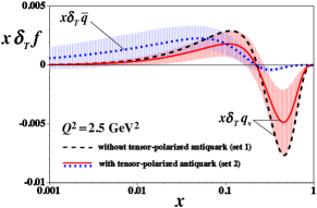
Figure 3: (Color online) Obtained tensor-polarized PDFs at $Q^{2}=2.5$ GeV². The solid and dashed curves indicate the tensor-polarized valence-quark distributions $x\delta_{T}q_{v}(x)$ with finite tensor-polarized antiquark distributions (set-2, $\alpha_{\bar{q}}\neq 0$) and without them (set-1, $\alpha_{\bar{q}}=0$), respectively. The dotted curve is the tensor-polarized antiquark distribution $x\delta_{T}\bar{q}(x)$ in the set-2 tensor-pdfs . The uncertainty bands of $\Delta\chi^{2}=1$ are shown.

Then, the determined tensor-polarized PDFs are shown in Fig. 3. The tensor-polarized valence-quark and antiquark distributions are shown for the set-2 by the solid and dotted curves, and the valence-quark distribution of the set-1 is shown by the dashed curves. All the distributions are negative at large $x$ ($>0.2$), and they turn into positive at the node point around $x\sim 0.2$. These are distributions at $Q^{2}=2.5$ GeV². Since these distributions are the only ones determined by the $\chi^{2}$ analysis of existing $b_{1}$ data in a model independent way, we use them for estimating the tensor-polarization asymmetry in proton-deuteron Drell-Yan process at Fermilab. However, one should note that the tensor-polaried PDFs are not determined well at this stage as shown by the error bands in Fig. 3, and future experimental progress is obviously needed for $b_{1}$. Only the uncertainty bands of $\Delta\chi^{2}=1$ are shown in Fig. 3. Hereafter, $\Delta\chi^{2}=1$ bands are shown in figures.

II.2 Polarized proton-deuteron Drell-Yan process with tensor-polarized deuteron

Polarized proton-proton Drell-Yan processes have been theoretically investigated extensively, and the studies are foundations for the RHIC (Relativistic Heavy Ion Collider)-spin project. However, polarized proton-deuteron processes have not been studied well partly because there was no actual experimental project. In 1990’s, a possible deuteron-beam polarization was considered for RHIC rhic-d ; however, it was not realized. On the other hand, the polarized proton-deuteron Drell-Yan processes are possible with a polarized deuteron target, and it is becoming a realistic project at Fermilab.

The formalisms of polarized proton-deuteron Drell-Yan processes were investigated in Ref. pd-drell-yan . The cross section for the Drell-Yan process $p+d\to\mu^{+}\mu^{-}+X$ is given by a lepton tensor multiplied by the hadron tensor

$$\!W_{\mu\nu}^{DY}\!=\!\frac{1}{4\pi M}\!\int\!d^{\,4}\xi\,e^{-i(k_{1}+k_{2})\cdot\xi}\langle\,p\,d\,|\,J_{\mu}^{\,em}(\xi)J_{\nu}^{\,em}(0)\,|\,p\,d\,\rangle,$$ (13)

where $k_{1}$ and $k_{2}$ are momenta for $\mu^{-}$ and $\mu^{+}$, respectively. The leading subprocess, which contributes to the cross section, is the quark-antiquark annihilation process $q\bar{q}\to\mu^{+}\mu^{-}$ shown in Fig. 4.

According to the general formalism for $W_{\mu\nu}^{DY}$ by using Hermiticity, parity conservation, and time-reversal invariance pd-drell-yan , there exist 108 structure functions in the proton-deuteron (pd) Drell-Yan processes instead of 48 functions in the proton-proton (pp) Drell-Yan. There are 60 new structure functions due to the spin-one nature of the deuteron. However, most of them are higher-twist functions and all of them are not important especially at the first stage. Because it is too lengthy to write these structure functions, we explain only the essential functions associated with the leading-twist part of the deuteron tensor structure.

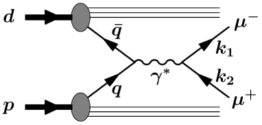
Figure 4: Typical Drell-Yan process.

In the pp Drell-Yan processes, there are spin asymmetries by combinations of the unpolarized state (U) together with longitudinal (L) and transverse (T) polarizations: $<\!\sigma\!>$, $A_{LL}$, $A_{TT}$, $A_{LT}$, and $A_{T}\,(\,=A_{UT},\,A_{TU})$. In the pd Drell-Yan, additional tensor-polarization asymmetries exist, and the following spin asymmetries could be investigated:

$$\!\!\!\!\!\!\!<\!\sigma\!>,\, A_{LL},\, A_{TT},\, A_{LT},\, A_{TL},\, A_{UT},\, A_{TU},\,$$

$$\!\!\!\!\!\!\!\,A_{UQ_{0}},\, A_{TQ_{0}},\, A_{UQ_{1}},\, A_{LQ_{1}},\, A_{TQ_{1}},\, A_{UQ_{2}},\, A_{LQ_{2}},\, A_{TQ_{2}},$$ (14)

where $Q_{0}$, $Q_{1}$, and $Q_{2}$ indicate three tensor polarizations depending on polarization direction pd-drell-yan ; sk14 . In particular, we investigate the tensor-polarization asymmetry

$$\!A_{UQ_{0}}\!=\!\frac{1}{2\!<\!\sigma\!>}\bigg{[}\sigma(\bullet,0_{L})-\frac{\sigma(\bullet,+1_{L})+\sigma(\bullet,-1_{L})}{2}\bigg{]},\!\!$$ (15)

in this work. Here, $\bullet$ indicates the unpolarized proton.

The Drell-Yan cross sections and spin asymmetries can be expressed in terms of PDFs. As shown in Fig. 5, the leading contribution to the hadron tensor is generally given by quark and antiquark correlation functions as

$$W_{\mu\nu}^{\,q\bar{q}}=\frac{1}{3}\sum_{a,b}\delta_{b\bar{a}}\,e_{a}^{2}\int d^{4}k_{a}\,d^{4}k_{b}\,\delta^{4}(k_{a}+k_{b}-Q)\,$$

$$\ \ \ \ \ \ \ \times\text{Tr}\left[\,\Phi_{a/p}(P_{1}S_{1};k_{a})\gamma_{\mu}\bar{\Phi}_{b/d}(P_{2}S_{2};k_{b})\gamma_{\nu}\,\right],$$ (16)

where $k_{a}$ and $k_{b}=k_{\bar{a}}$ are quark and antiquark momenta, the color average and summations are taken by $3\cdot(1/3)^{2}$, and the correlation functions $\Phi_{a/p}$ and $\bar{\Phi}_{\bar{a}/d}$ are defined by the quark field $\psi$ as

$$\!\left(\Phi_{a/p}\right)_{ij} =\!\!\int\!\frac{d^{4}\xi}{(2\pi)^{4}}\,e^{ik_{a}\cdot\xi}\,\langle\,P_{1}S_{1}\,|\,\bar{\psi}_{j}^{(a)}(0)\,\psi_{i}^{(a)}(\xi)\,|\,P_{1}S_{1}\,\rangle,$$

$$\!\left(\bar{\Phi}_{\bar{a}/d}\right)_{ij} =\!\!\int\!\frac{d^{4}\xi}{(2\pi)^{4}}\,e^{ik_{\bar{a}}\cdot\xi}\,\langle\,P_{2}S_{2}\,|\,\psi_{i}^{(a)}(0)\,\bar{\psi}_{j}^{(a)}(\xi)\,|\,P_{2}S_{2}\,\rangle.$$ (17)

Here, link operators for satisfying the gauge invariance are not explicitly written. The correlation functions are expressed by unpolarized, longitudinally-polarized, transversity distributions, and new tensor-polarized distributions. There is another contribution obtained by exchanging quark and antiquark ($W_{\mu\nu}^{\,\bar{q}q}$).

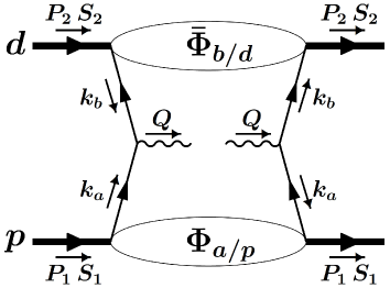
Figure 5: Parton model for Drell-Yan process.

Now, we express the Drell-Yan cross section, structure functions, and the tensor-polarization asymmetry in the parton model. There are 19 structure functions for the proton-deuteron Drell-Yan in the parton model; however, the number becomes four after the integration over the transverse momentum of $Q$. Denoting $\overline{F}=\int d^{2}Q_{T}F$ for the structure function $F$, we have the pd Drell-Yan cross section pd-drell-yan :

$$\frac{d\sigma}{dx_{1}\,dx_{2}\,d\Omega} =\frac{\alpha^{2}}{4\,Q^{2}}\,\bigg{[}\,(1+\cos^{2}\theta)\bigg{\{}\,\overline{W}_{T}+\frac{1}{4}\lambda_{1}\lambda_{2}\,\overline{V}_{T}^{\,LL}$$

$$\ \ \ \ \ \ \ \ \ \ \ +\frac{2}{3}\left(2\,|\vec{S}_{1T}|^{2}-\lambda_{1}^{2}\right)\,\overline{V}_{T}^{\,UQ_{0}}\,\bigg{\}}$$

$$\!\!\!\!\!\!\!\!\!\!\!\!\!\!\!\!\!+\sin^{2}\theta\,|\vec{S}_{1T}|\,|\vec{S}_{2T}|\cos(2\phi-\phi_{1}-\phi_{2})\,\overline{U}_{2,2}^{\,TT}\,\bigg{]},$$ (18)

where $\theta$ and $\phi$ are polar and azimuthal angles of the vector $\vec{k}_{1}-\vec{k}_{2}$ for the dimuon, $\lambda_{1}$ and $\lambda_{2}$ are proton and deuteron helicities, and $\vec{S}_{1T}$ and $\vec{S}_{2T}$ are the transverse spin vectors for the proton and deuteron defined by the angle $\phi_{1}$ and $\phi_{2}$ as $\vec{S}_{1T}=|\vec{S}_{1T}|\,(\cos\phi_{1},\,\sin\phi_{1},\,0)$, $\vec{S}_{2T}=|\vec{S}_{2T}|\,(\cos\phi_{2},\,\sin\phi_{2},\,0)$. The variables $x_{1}$ and $x_{2}$ are lightcone momentum fractions for the partons in the proton and deuteron, respectively. Neglecting hadron masses and transverse momentum of the dimuon, we have the relation $Q^{2}=M_{\mu\mu}^{2}=x_{1}x_{2}s$ field-book . The rapidity of the muon pair is given by $y=(1/2)\ln((E_{\mu\mu}+P_{\mu\mu,L})/(E_{\mu\mu}-P_{\mu\mu,L}))=(1/2)\ln(x_{1}/x_{2})$, where $E_{\mu\mu}$ and $P_{\mu\mu,L}$ are dimuon energy and longitudinal momentum. The momentum fractions $x_{1}$ and $x_{2}$ are expressed by these external variables as $x_{1}=\sqrt{\tau}e^{y}$ and $x_{2}=\sqrt{\tau}e^{-y}$. The dimuon transverse momentum is generally small in comparison with the dimuon mass in the Fermilab experiment Fermilab-MI . In the parton model, the structure functions are expressed by the parton distributions for the process $q+\bar{q}\rightarrow\mu^{+}+\mu^{-}$ as

$$\overline{W}_{T} =\frac{1}{3}\sum_{i}e_{i}^{2}\,q_{i}(x_{1},Q^{2})\,\bar{q}_{i}(x_{2},Q^{2})+(q\leftrightarrow\bar{q}),$$

$$\overline{V}_{T}^{\,LL} =-\frac{4}{3}\sum_{i}e_{i}^{2}\,\Delta q_{i}(x_{1},Q^{2})\,\Delta\bar{q}_{i}(x_{2},Q^{2})+(q\leftrightarrow\bar{q}),$$

$$\overline{U}_{2,2}^{\,TT} =\frac{1}{3}\sum_{i}e_{i}^{2}\,\Delta_{{}_{T}}q_{i}(x_{1},Q^{2})\,\Delta_{{}_{T}}\bar{q}_{i}(x_{2},Q^{2})+(q\leftrightarrow\bar{q}),$$

$$\!\!\overline{V}_{T}^{\,UQ_{0}} =\frac{1}{6}\sum_{i}e_{i}^{2}\,q_{i}(x_{1},Q^{2})\,\delta_{{}_{T}}\bar{q}_{i}(x_{2},Q^{2})+(q\leftrightarrow\bar{q}),$$ (19)

where $\Delta q_{i}$ and $\Delta_{{}_{T}}q_{i}$ are longitudinally-polarized and transversity distributions. The terms $(q\leftrightarrow\bar{q})$ indicate the contributions from $\bar{q}$(in p)+$q$(in d)$\rightarrow\mu^{+}+\mu^{-}$ by the replacements $q\leftrightarrow\bar{q}$ in the first terms.

In this article, we are interested in investigating the tensor-polarization asymmetry $A_{UQ_{0}}$ of Eq. (15), and it is expressed in the parton model as pd-drell-yan ; sk14

$$A_{Q}\equiv 2A_{UQ_{0}}=\frac{2\,\overline{V}_{T}^{\,UQ_{0}}}{\overline{W}_{T}}$$

$$\!\!\!\!\!\!=\frac{\sum_{i}e_{i}^{2}\,\left[\,q_{i}(x_{1},Q^{2})\,\delta_{{}_{T}}\bar{q}_{i}(x_{2},Q^{2})+\bar{q}_{i}(x_{1},Q^{2})\,\delta_{{}_{T}}q_{i}(x_{2},Q^{2})\,\right]}{\sum_{i}e_{i}^{2}\,\left[\,q_{i}(x_{1},Q^{2})\,\bar{q}_{i}(x_{2},Q^{2})+\bar{q}_{a}(x_{1},Q^{2})\,q_{i}(x_{2},Q^{2})\,\right]},$$ (20)

where the factor of 2 is multiplied to define $A_{Q}$ delta-T-notation so that the asymmetry becomes the simple ratio of the unpolarized PDFs $f(x)$ and the tensor-polarized PDFs $\delta_{T}f(x)$, although there is nothing wrong in the formalism of Ref. pd-drell-yan . The scale $Q^{2}$ is given by the dimuon mass $Q^{2}=M_{\mu\mu}^{\,2}=(k_{1}+k_{2})^{2}=(k_{a}+k_{b})^{2}=x_{1}\,x_{2}\,s$, the unpolarized PDFs $f(x,Q^{2})$ and tensor-polarized PDFs $\delta_{T}f(x,Q^{2})$ should be obtained at this $Q^{2}$ scale for estimating the asymmetry $A_{Q}$. The unpolarized PDFs are well known, and we could use the available parametrization for the tensor-polarized PDFs in Eq. (9) and Fig. 3 for our numerical calculations of $A_{Q}$.

III Results

Because the tensor-polarized PDFs are obtained at $Q^{2}=2.5$ GeV² in Eq. (9), they need to be evolved to the $Q^{2}$ points of the Fermilab Drell-Yan experiment. The proton beam energy is $E_{p}=120$ GeV for the Fermilab Main Injector (MI), so that the center-of-mass energy squared is $s=(p_{1}+p_{2})^{2}=M_{p}^{2}+M_{d}^{2}+2M_{d}E_{p}$ in the proton-deuteron Drell-Yan process with the proton (deuteron) four momentum $p_{1}$ ($p_{2}$) and its mass $M_{p}$ ($M_{d}$). Then, the dimuon mass $M_{\mu\mu}$, which is equal to $Q^{2}$, is given by $Q^{2}=M_{\mu\mu}^{2}=x_{1}x_{2}s$. So far, the dimuon-mass region of $4^{2}$ GeV²$<M_{\mu\mu}^{2}<9^{2}$ GeV² is measured between the $J/\psi$ and $\Upsilon$ resonances. Therefore, the $Q^{2}$ evolution of the tensor-polarized PDFs are necessary for estimating the tensor-polarization asymmetry for the Fermilab experiment.

III.1 Scale dependence of the tensor-polarized
parton distribution functions

The $Q^{2}$ evolution of $b_{1}$ and the tensor-polarized PDFs is rarely discussed, so that we briefly mention it here along the explanation of Ref. hjm89 . The operator product expansion (OPE) was studied within the twist-two level, and the time-ordered product of two electromagnetic currents is expressed by twist-two vector and axial-vector operators, $O_{V}^{\,\mu_{1}\cdots\mu_{n}}$ and $O_{A}^{\,\mu_{1}\cdots\mu_{n}}$. The vector operators are defined by the quark field $\psi$ and the covariant derivative $D^{\,\mu}$ as

$$\!O_{V}^{\,\mu_{1}\cdots\mu_{n}}=\frac{1}{2}\left(\frac{i}{2}\right)^{n-1}\!\!\!S\left[\,\overline{\psi}\,\gamma^{\,\mu_{1}}\overset{\text{\scriptsize$\leftrightarrow$}}{D}\,^{\mu_{2}}\cdots\overset{\text{\scriptsize$\leftrightarrow$}}{D}\,^{\mu_{n}}\,e_{q}^{\,2}\,\psi\,\right],$$ (21)

where $S$ indicates the symmetrization of the indices ($\mu_{1}\cdots\mu_{n}$) and removal of the trace. The structure functions $F_{1,2}$ and $b_{1,2}$ can be obtained from the vector operators $O_{V}^{\,\mu_{1}\cdots\mu_{n}}$, whose matrix elements are expressed as

$$\left.\langle\,p,E\,\right|\,O_{V}^{\mu_{1}\cdots\mu_{n}}\,\left|\,p,E\,\rangle\right.=S\bigg{[}\,a_{n}p^{\,\mu_{1}}\cdots p^{\,\mu_{n}}$$

$$\ \ \ \ \ \ \ +d_{n}\left(E^{*\mu_{1}}E^{\,\mu_{2}}-\frac{1}{3}\,p^{\,\mu_{1}}p^{\,\mu_{2}}\right)\,p^{\,\mu_{3}}\cdots p^{\,\mu_{n}}\,\bigg{]}.$$ (22)

The coefficients $a_{n}$ and $d_{n}$ are associated with the structure functions $F_{1}$ and $b_{1}$, respectively. Therefore, as explained in Ref. hjm89 , the $b_{1}$ and $b_{2}$ are obtained from the same vector operators $O_{V}^{\,\mu_{1}\cdots\mu_{n}}$. Then, their anomalous dimensions and also coefficient functions in the OPE are common in $F_{1,2}$ and $b_{1,2}$, so that the $Q^{2}$ evolutions of $b_{1,2}$ are the same as the ones for $F_{1,2}$. Namely, the $Q^{2}$ evolution of the tensor-polarized PDFs is calculated by the same DGLAP (Dokshitzer-Gribov-Lipatov-Altarelli-Parisi) evolution equations with the replacement of the unpolarized PDFs by the tensor-polarized PDFs. Therefore, the DGLAP $Q^{2}$-evolution code, for example in Ref. bf1 , can be used for calculating $Q^{2}$ variations of the tensor-polarized PDFs.

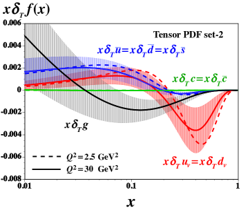
Figure 6: (Color online) $Q^{2}$ evolution results of set-2 tensor-polarized PDFs are shown. The dashed curves are the initial distributions at $Q^{2}=2.5$ GeV², and the solid curves indicate the tensor-polarized PDFs at $Q^{2}=30$ GeV².

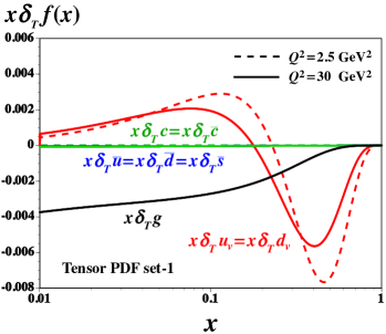
Figure 7: (Color online) $Q^{2}$ evolution results of set-1 tensor-polarized PDFs are shown. The dashed curves are the initial distributions at $Q^{2}=2.5$ GeV², and the solid curves indicate the tensor-polarized PDFs at $Q^{2}=30$ GeV².

The tensor-polarized PDFs in Eq. (9) and Fig. 3 at $Q^{2}=2.5$ GeV² are evolved to the $Q^{2}$ points, $Q^{2}=M_{\mu\mu}^{2}=x_{1}x_{2}s$, for the Fermilab-MI kinematics by the standard DGLAP evolution equations bf1 . At the initial scale of $Q_{0}^{2}=2.5$ GeV², the tensor-polarized charm and gluon distributions are assumed to be zero: $\delta_{T}c(x,Q_{0}^{2})=\delta_{T}\bar{c}(x,Q_{0}^{2})=\delta_{T}g(x,Q_{0}^{2})=0$. The uncertainties of the evolved PDFs are shown by the bands for $\Delta\chi^{2}=1$, and the uncertainty of the gluon distribution is also estimated. The evolution results of the set-2 tensor-polarized PDFs are shown in Fig. 6 from the initial $Q^{2}=2.5$ GeV² to $Q^{2}=30$ GeV², which roughly corresponds to a typical $Q^{2}$ value of the Fermilab experiment. Within this $Q^{2}$ variation, the PDFs do not change significantly although the node position moves from $x=0.22$ to $0.16$. However, it is interesting to find a significant tensor-polarized gluon distribution $\delta_{T}g(x)$ due to the $Q^{2}$ evolution although it is zero in the initial scale, and its $x$ dependence is much different from the quark and antiquark distributions. We use the evolution results at $Q^{2}=x_{1}x_{2}s$ for given $x_{1}$ and $x_{2}$ for calculating the tensor-polarized spin asymmetries at Fermilab in the next subsection. For comparison, the evolution results of the set-1 tensor-polarized PDFs are shown in Fig. 7. Here, there is no antiquark tensor-polarization at the initial scale $Q^{2}=2.5$ GeV². Finite tensor-polarized antiquark distributions are obtained at $Q^{2}=30$ GeV² due to the $Q^{2}$ evolution; however, they are still tiny as shown in the figure. Because the Drell-Yan cross section is sensitive to the antiquark distributions, it leads to small tensor-polarization asymmetries. At this stage, the set-2 distributions are more realistic ones because they can explain the HERMES measurements. It is also interesting to find a significant tensor-polarized gluon distribution although the antiquark distributions are very small in the set-1 parametrization.

III.2 Tensor-polarization asymmetry
in proton-deuteron Drell-Yan process

We show the obtained tensor-polarization asymmetries $A_{Q}$ in Fig. 8 at $x_{1}=0.2$, 0.4, and 0.6. There are two-sets of tensor-polarized PDFs as shown in Eq. (9) and Fig. 3. The tensor-polarized PDFs are evolved from $Q^{2}=2.5$ GeV² to the scale $Q^{2}=M_{\mu\mu}^{\,2}=x_{1}x_{2}s$ by taking the proton energy $E_{p}=120$ GeV with the fixed-target deuteron for the Fermilab-MI experiment. Since the MSTW2008 unpolarized LO (leading order) PDFs were used in the $b_{1}$ analysis tensor-pdfs , the MSTW2008-LO code MSTW2008 is used for calculating the unpolarized PDFs at the same $Q^{2}$ points. There are small nuclear corrections, usually within a few percent, in the unpolarized PDFs for the deuteron hkn07 , but they are neglected in this work. In showing the curves, the experimental kinematical cut $4^{2}<M_{\mu\mu}^{\,2}<9^{2}$ GeV² is not applied except for the condition $Q^{2}=M_{\mu\mu}^{\,2}>2.5$ GeV². If $x_{1}$ is large, the large $x_{2}$ region cannot be reached in the Fermilab experiment because of the condition $4^{2}<M_{\mu\mu}^{\,2}<9^{2}$ GeV².

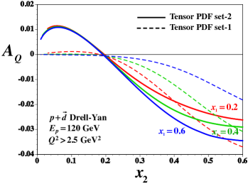
Figure 8: (Color online) Tensor-polarization asymmetries $A_{Q}$ are shown for $x_{1}=0.2$, 0.4 and 0.6 by using two sets of tensor polarized PDFs. The dashed curves are for the set-1 without the tensor-polarized antiquark distributions at the initial scale ($Q^{2}=2.5$ GeV²), the solid curves indicate the set-2 results.

We find in Fig. 8 that the tensor-polarization asymmetry $A_{Q}$ is generally of the order of a few percent. The set-1 asymmetries are rather small because the antiquark tensor polarization does not exist at $Q^{2}=2.5$ GeV², and it appears only by the $Q^{2}$ evolution. The set-2 asymmetries are generally much larger. We believe that the set-2 results are more reliable at this stage because they can explain the HERMES measurements including the small-$x$ region as shown in Fig. 2. Since the HERMES $b_{1}$ data are taken in the region $0.012<x<0.452$, our predictions should be reasonable ones for the symmetries in the Fermilab experiment, where the kinematical region $0.1<x_{2}<0.5$ will be probed. There are large differences in asymmetries between set-1 and set-2. However, in other words, it indicates the importance to measure tensor-polarization asymmetry because it is the advantage of the Drell-Yan experiment to probe the antiquark distributions. Shadowing effects are effectively included in the HERMES data at small $x$, possibly at $x<0.05$, our predictions include such effects in the set-2. However, the Fermilab experiment is not sensitive to the small $x_{2}$ region ($x_{2}<0.05$), so that we may wait for the electron-on collider project eic for small-$x$ measurements to probe shadowing effects on $b_{1}$.

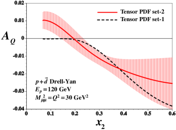
Figure 9: (Color online) Tensor-polarization asymmetries $A_{Q}$ are shown at the fixed $M_{\mu\mu}^{\,2}=Q^{2}=30$ GeV² by using two sets of tensor polarized PDFs. The dashed curve is for the set-1 without the tensor-polarized antiquark distributions at the initial scale ($Q^{2}=2.5$ GeV²), the solid curve indicates the set-2 results. The uncertainty band is shown for the set-2 curve.

One thing we need to check is the uncertainty of the tensor-polarized PDFs in showing the asymmetries because they are not well determined as shown in Figs. 3 and 6. We show the uncertainties for the set-2 at fixed $M_{\mu\mu}^{2}=Q^{2}=30$ GeV² in Fig. 9. There are large differences in the asymmetries between set-1 and set-2; however, they are mostly within the error bands, whereas the set-1 curve at small $x_{2}(<0.2)$ is outside of the $\Delta\chi^{2}=1$ band. This small-$x_{2}$ discrepancy is caused by the difference in handing the antiquark distributions at $x<0.2$ originally in Fig. 3. Although the error bands are large, we predict a finite tensor-polarized asymmetry which could be investigated at Fermilab or other hadron facilities.

In Eq. (8), we mentioned that tensor-polarized antiquark distributions are important to be measured for finding a possible mechanism on the tensor structure in quark and gluon degrees of freedom. Therefore, the Drell-Yan measurement is a valuable experiment which is very likely to create a new field of hadron physics. It is complementary to the JLab $b_{1}$ experiment which will start in a few years. There is also a plan to measure the tensor polarization $A_{zz}$ at JLab in the large-$x$ region azz , and $b_{1}$ could be measured at EIC eic .

Historically, the Fermilab Drell-Yan experiment played a crucial role in establishing the flavor asymmetric antiquark distributions $\bar{u}\neq\bar{d}$ flavor3 . This flavor asymmetry was suggested in the NMC (New Muon Collaboration) experiment by the violation of the Gottfried sum rule; however, it was not obvious whether the NMC experiment could be interpreted by a small-$x$ contribution without the flavor asymmetric distributions. This issue was clarified by the Fermilab Drell-Yan experiment on the cross section ratio $\sigma_{pd}^{DY}/(2\sigma_{pp}^{DY})$, which directly probed $\bar{u}\neq\bar{d}$. In the same way, the tensor-polarized Drell-Yan experiment should be valuable for probing the antiquark tensor polarization directly. Hopefully, such an experiment will be done at Fermilab. In addition, it could be done at any facilities with high-energy hadron beams such as BNL (Brookhaven National Laboratory)-RHIC, CERN-COMPASS, J-PARC (Japan Proton Accelerator Research Complex) j-parc , GSI-FAIR (Gesellschaft für Schwerionenforschung -Facility for Antiproton and Ion Research), and IHEP (Institute for High Energy Physics) in Russia.

IV Summary

There exist new polarized structure functions for spin-one hadrons such as the deuteron. In particular, the twist-two structure functions $b_{1}$ and $b_{2}$ of charged-lepton DIS are expressed in terms of tensor-polarized PDFs. These functions could probe peculiar nature of hadrons in the sense that they should vanish if the internal constituents are in the S-wave and that HERMES $b_{1}$ measurements are much larger than the conventional deuteron-model estimate.

New accurate measurements are planned at JLab by the electron DIS with the tensor-polarized deuteron. Furthermore, a Fermilab Drell-Yan experiment is now under consideration with the fixed tensor-polarized deuteron target. For pursuing this experiment and allocating beam time at Fermilab, it is crucial to estimate the magnitude of a possible tensor-polarization asymmetry theoretically. Using the optimum tensor-polarized PDFs obtained by analyzing the HERMES data, we estimated the tensor-polarization asymmetry by considering the Fermilab kinematics. We found that the asymmetry $A_{Q}$ is of the order of a few percent.

It is a small quantity; however, we believe that it is worth for the measurement to find the physics mechanisms of tensor polarization in the parton level. Especially, the Drell-Yan experiment should provide important information on the tensor-polarized antiquark distributions. It could lead to a new field of high-energy spin physics to probe an exotic aspect in hadrons. Furthermore, we showed in our analysis that a finite tensor-polarized gluon distribution should exist, and it has never been studied experimentally. It is also an interesting future topic.