The Alcock Paczyński test with Baryon Acoustic Oscillations: systematic effects for future surveys

Abstract

We investigate the Alcock Paczyński (AP) test applied to the Baryon Acoustic Oscillation (BAO) feature in the galaxy correlation function. By using a general formalism that includes relativistic effects, we quantify the importance of the linear redshift space distortions and gravitational lensing corrections to the galaxy number density fluctuation. We show that redshift space distortions significantly affect the shape of the correlation function, both in radial and transverse directions, causing different values of galaxy bias to induce offsets up to 1% in the AP test. On the other hand, we find that the lensing correction around the BAO scale modifies the amplitude but not the shape of the correlation function and therefore does not introduce any systematic effect. Furthermore, we investigate in details how the AP test is sensitive to redshift binning: a window function in transverse direction suppresses correlations and shifts the peak position toward smaller angular scales. We determine the correction that should be applied in order to account for this effect, when performing the test with data from three future planned galaxy redshift surveys: Euclid, the Dark Energy Spectroscopic Instrument (DESI) and the Square Kilometer Array (SKA).

1 Introduction

With the measurements of Cosmic Microwave Background (CMB) anisotropies, performed by WMAP [1] and Planck [2] experiments, cosmology has entered a precision era, leading to the confirmation of $\Lambda$CDM as the standard model for cosmology. Despite the stunning agreement between theory and data that has been reached, still many open questions remain to be investigated within the standard model. One of these unsolved puzzles is the accelerated expansion of the universe [3], which in the standard cosmological model is driven by a cosmological constant $\Lambda$, whose value leads to a serious fine-tuning problem and a coincidence problem [4, 5]. Therefore many alternative models with dynamical dark energy or modifications of General Relativity which can lead to the same accelerated expansion as $\Lambda$CDM have been proposed [6]. A crucial role in shedding light on the nature and origin of cosmic acceleration will be played in the next decades by Large Scale Structure (LSS) experiments, which will quantify the impact of Dark Energy in the growth of cosmic structures. Different tracers of cosmic structures will provide information on different stages of the expansion history.

In this work we focus on galaxy clustering. The upcoming galaxy surveys will map the distribution of galaxies on a large fraction of the sky up to redshift $z\sim 2$. In order to exploit this huge amount of incoming data, an accurate model for what we will be measuring in galaxy surveys is required. Moreover, having much better statistics, we may release some of the assumptions and proceed in a more model independent way.

In the past few years, the galaxy number counts have been computed including all the relativistic effects at the linear order [7, 8, 9, 10] and at second order [11, 12, 13] in perturbation theory. Besides the known redshift space distortions correction to the local overdensity of galaxies [14], other terms contribute to galaxy number counts, e.g. Doppler corrections and gravitational lensing. Not taking into account these effects in our theoretical model may bias the analysis [15], therefore their relevance in any cosmological observable should be tested.

On relatively small scales, other effects such as the non-linear redshift space distortions (the so called "finger of god" effect) may be relevant. In this work we do not model these distortions. We focus on the regime of large scales, where linear theory is assumed to be a good approximation.

In this paper we will investigate the relevance of these corrections for the Alcock Paczyński (AP) test [16]. We start from the method proposed in [17], where the AP test is performed on the Baryon Acoustic Oscillation (BAO) feature of the galaxy 2-point correlation function without any prior assumption on the cosmological parameters. Nevertheless, we will show that some prior information about the galaxy bias can improve the accuracy in determining the BAO scale from the observable quantities.

In Section 2 we introduce the formalism we employ throughout the paper for the observed galaxy number density. In Section 3 we present the AP test and we introduce the AP parameter. In Section 4 we summarize the method we use to compute the galaxy 2-point correlation function and to determine the position of the acoustic peak and we outline the general strategy to investigate observational distortions of the test. More details on the methodology are given in Appendix A. In Section 5 we report our results: in 5.1, we discuss the relevance of the relativistic correction to the galaxy number count for the AP test, in 5.2 we introduce a linear local bias and we show how it affects our method; in 5.3 we study projection effects induced by a radial window function and we compute the corrective factors that must be applied to the estimated AP parameter for three future planned galaxy surveys, i.e. Euclid [18], the Dark Energy Spectroscopic Instrument (DESI) [19] and the Square Kilometer Array (SKA) [20]. We also analyze the impact of shot-noise and cosmic variance on the accuracy of the BAO peak determination in Section 5.4. In Section 6 we draw the conclusions.

2 Relativistic formalism for galaxy correlations

We consider a Friedmann universe with linear scalar perturbations. We work in Newtonian gauge so that the line element is given by

$$ds^{2}=a(t)^{2}\left(-\left(1+2\Psi\right)dt^{2}+\left(1-2\Phi\right)d{\mathbf{x}}^{2}\right)\,,$$ (2.1)

where $a(t)$ is the scale factor, $t$ is conformal time and the metric perturbations, $\Psi$ and $\Phi$, are the Bardeen potentials. We remark that working solely with observational quantities, we can fix the gauge without loss of generality.

Galaxies are discrete tracers of the density field of the universe. In order to obtain cosmological information from the analysis of their distribution, it is crucial to identify the true observable in galaxy surveys and how the large scale dark matter distribution, that we cannot directly observe, is mapped into observable coordinates. The true observable in galaxy surveys, the galaxy number density fluctuation $\Delta_{\text{obs}}$, has been computed at first order in perturbation theory using a relativistic formalism by tracing the photons path between the source and the observer [7, 8, 9, 10]. These are expressed as functions of the observed redshift of the source $z$ and the direction of propagation of the emitted photons ${\mathbf{n}}$. It includes a local density field term plus additional terms due to fact that measured redshift $z$ and angular position (${\mathbf{n}}$) are perturbed by velocity and metric perturbations at the source position and by the intervening gravitational potentials between the source and the observer.

The total observed galaxy overdensity $\Delta_{\text{obs}}\left({\mathbf{n}},z\right)$ can be schematically expressed as a sum of different contributions

$$\Delta_{\text{obs}}=\Delta_{g}+\Delta_{\text{RSD}}+\Delta_{\kappa}+\Delta_{\text{rel}},$$ (2.2)

where $\Delta_{g}$ is the local galaxy overdensity,

$$\Delta_{g}=b\ \delta$$ (2.3)

proportional to the density contrast in comoving gauge $\delta$. For the sake of simplicity, we assume the bias $b$ to be linear and local. The term $\Delta_{\text{RSD}}$ in our notation includes the linear redshift space distortions contributions, due to the peculiar motion of galaxies, plus other subdominant Doppler corrections [21]

$$\Delta_{\text{RSD}}(\mathbf{n},z)=\frac{1}{\mathcal{H}(z)}\partial_{r}(\mathbf{V}\cdot\mathbf{n})+\Biggl{(}\frac{\mathcal{H^{\prime}}}{\mathcal{H}^{2}}+\frac{2}{r\mathcal{H}}\Biggr{)}(\mathbf{V}\cdot\mathbf{n})-3{\cal H}V,$$ (2.4)

where $\mathbf{V}$ is the peculiar velocity in longitudinal gauge, $V$ the potential velocity defined by ${\bf V}=-{\bf\nabla}V$, $r=t_{o}-t$ is the conformal distance and $\mathcal{H}=a^{\prime}/a$ is the conformal Hubble factor and a prime denotes a derivative with respect to the conformal time $t$. $\Delta_{\kappa}$ is the gravitational lensing term,

$$\Delta_{\kappa}=-\int_{0}^{r(z)}\frac{r(z)-r}{r(z)r}\Delta_{\Omega}(\Phi+\Psi)dr,$$ (2.5)

where $\Delta_{\Omega}$ is the Laplace operator on the sphere. The last term in Eq. (2.2), $\Delta_{\rm rel},$ includes subdominant local and integrated combinations of the Bardeen potentials:

$$\Delta_{\rm rel}= -2\Phi+\Psi+\frac{1}{\mathcal{H}}\Phi^{\prime}+\frac{2}{r(z)}\int^{r(z)}_{0}dr(\Phi+\Psi)+$$

$$+\Biggl{(}\frac{\mathcal{H^{\prime}}}{\mathcal{H}^{2}}+\frac{2}{r(z)\mathcal{H}}\Biggr{)}\Biggl{(}\Psi+\int^{r(z)}_{0}dr(\Phi^{\prime}+\Psi^{\prime})\Biggr{)}\,.$$ (2.6)

Throughout this work we will neglect the effect of magnification bias and the possible evolution of the number of counts [10]. Even if present, these bias factors multiply terms which are subdominant in the AP test.

(a) Transverse correlation function

(b) Longitudinal correlation function

Figure 1: Transverse and longitudinal correlation function computed at $z_{\rm mean}=1.5$, partially including the corrective terms in Eq. (2.2). In the bottom panels, we show the relative differences between the exact correlation function (including all the terms) and a partial correlation function computed including only the local density term (green, dashed line), density and redshift space distortion correction (red, dash-dotted line), the previous terms plus the lensing (blue, dotted line).

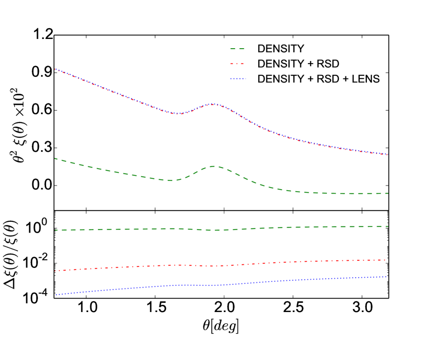
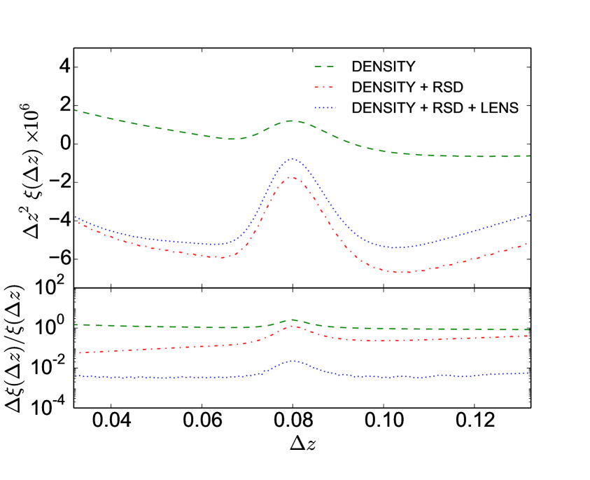
In terms of observational coordinates, the relevant statistical quantities are the angular correlation function $\xi(\theta,z_{1},z_{2})$ or the redshift dependent angular power spectra $C_{\ell}(z_{1},z_{2})$. The galaxy correlation function, under the assumption of statistical isotropy, reduces to

$$\xi(\theta,z_{1},z_{2})=\left<\Delta_{\text{obs}}(\mathbf{n}_{1},z_{1})\Delta_{\text{obs}}(\mathbf{n}_{2},z_{2})\right>,\qquad\cos{\theta}\equiv\mathbf{n_{1}}\cdot\mathbf{n_{2}},$$ (2.7)

where $\langle..\rangle$ denotes the ensemble average over several realizations. Observationally, this is replaced by an average over directions at fixed observed redshift and opening angle $\theta$. In a similar way, the angular power spectrum is defined as [9]

$$C_{\ell}(z_{1},z_{2})=\left<a_{\ell m}(z_{1})a^{*}_{\ell m}(z_{2})\right>,$$ (2.8)

where a star denotes the complex conjugate and $a_{\ell m}$ are the coefficients of the spherical harmonic expansion for $\Delta(\mathbf{n},z)$

$$\Delta_{\text{obs}}(\mathbf{n},z)=\sum_{\ell m}a_{\ell m}(z)Y_{\ell m}(\mathbf{n}),\qquad a_{\ell m}\left(z\right)=\int d\Omega_{\mathbf{n}}Y^{*}_{\ell m}(\mathbf{n})\Delta_{\text{obs}}(\mathbf{n},z).$$ (2.9)

The angular power spectra and the correlation functions are related by

$$\xi(\theta,z_{1},z_{2})=\frac{1}{4\pi}\sum_{\ell=0}^{\infty}(2\ell+1)C_{\ell}(z_{1},z_{2})P_{\ell}(\cos{\theta}),$$ (2.10)

where $P_{\ell}(\cos{\theta})$ is the Legendre polynomial of degree $\ell$. From Eq. (2.10) it is straightforward to define the correlation function along the line-of-sight direction by setting $\theta=0$ and in the transverse direction by setting $z_{1}=z_{2}$.

The correlation function at a given mean redshift $z_{\text{mean}}$ along the line-of-sight is given by

$$\xi_{\parallel}(\Delta z,z_{\text{mean}})=\frac{1}{4\pi}\sum_{\ell=0}^{\infty}(2\ell+1)C_{\ell}(z_{\text{mean}}-\Delta z/2,z_{\text{mean}}+\Delta z/2)$$ (2.11)

while the transverse correlations are

$$\xi_{\perp}(\theta,z_{\text{mean}})=\frac{1}{4\pi}\sum_{\ell=0}^{\infty}(2\ell+1)C_{\ell}(z_{\text{mean}},z_{\text{mean}})P_{\ell}(\cos{\theta}).$$ (2.12)

Here $z_{\text{mean}}=(z_{1}+z_{2})/2$ and $\Delta z=z_{2}-z_{1}$.

Figure 1 represents transverse and longitudinal correlation function at fixed mean redshift $z_{\text{mean}}=1.5$. In each plot the correlation function is computed gradually adding subdominant contributions. Redshift-space distortions affect considerably the correlations in both directions, while lensing does not change sensitively the transverse correlations. In the longitudinal direction, the lensing term enhances the amplitude of the correlation function by up to 30% for $\Delta z\stackrel{{\scriptstyle<}}{{\sim}}0.13$, but it does not modify its shape at the BAO scale. We notice that the lensing effect is more important for pairs of galaxies with large radial separation. The contribution from the relativistic terms, i.e. Eq. (2.6), is completely subdominant and it would not be visible in Figure 1. Therefore we neglect it in the analysis performed in the rest of the paper. We remark that the largest relativistic correction, namely the Doppler term, is included in the redshift space distortions, see Eq. (2.4).

3 The Alcock Paczyński test

The Alcock Paczyński test [16], proposed for the first time in 1979, is a purely geometrical test of the cosmic expansion history performed by measuring the shape of an object expanding with the Hubble flow. When we observe an astrophysical object, we measure its shape in terms of its angular size $\theta$ and its radial extent in redshift space $\Delta z$. These two quantities depend on the comoving sizes of the source, $L_{\parallel}$ and $L_{\perp}$, and on a conversion factor: $\Delta z$ is related to the Hubble expansion rate $H\left(z\right)$ by

$$\Delta z=L_{\parallel}H(z),$$ (3.1)

while the dependence of $\theta$ on the angular diameter distance is given by

$$\theta=\frac{L_{\perp}}{(1+z)D_{A}(z)}.$$ (3.2)

If the object is known to be spherically symmetric, i.e. $L=L_{\perp}=L_{\parallel}$, then the ratio of these two measured quantities,

$$F_{\rm AP}\equiv\frac{\Delta z}{\theta},$$ (3.3)

does not depend on the physical size of the object, but only on the redshift and on the spacetime geometry

$$F_{\rm th}(z)=(1+z)D_{A}(z)H(z).$$ (3.4)

Here we explicitly distinguished the measured AP parameter $F_{\rm AP}$ from its theoretical (background) value $F_{\rm th}$.

In realistic applications, the spherical symmetry is not required to hold for single objects because the test can be applied to the galaxy clustering statistics. In fact, statistical isotropy of space implies statistical spherical symmetry for the correlation function. Furthermore, the correlation function naturally offers a robust feature for the application of the AP test, the BAO scale. BAO high-precision measurements are one of the main target of future spectroscopic surveys (see [22] for a recent overview of the cosmological implication of BAO measurements).

The application of the AP test on the BAO feature in the galaxy correlation function has been proposed in [17], where it has been found that the peak position of the transverse correlation function is significantly affected by the binning in redshift. This effect is due to the fact that a radial window for the transverse correlation function introduces a spurious radial component in the correlation function and the BAO peak estimation must be properly corrected for. In this paper we aim to extend the work presented in [17], addressing also other effects that may distort the result of the test.

4 Methodology

We assume a $\Lambda$CDM cosmology consistent with the best fit parameters from the Planck 2015 data [2]: $h=0.6774$, $\Omega_{cdm}h^{2}=0.1188$, $\Omega_{b}h^{2}=0.0223$, $\Omega_{\Lambda}=1-\Omega_{m}$, $\Omega_{k}=0$. The primordial amplitude and spectral index are set to $A_{s}=2.142\times 10^{-9}$ and $n_{s}=0.9667$.

The computation of the angular power spectrum for the observed galaxy number counts is implemented in the publicly available Boltzmann code classgal [23], a modified version of the Cosmic Linear Anisotropy Solving System (class) code [24, 25] optimized to compute accurately and efficiently the relativistic large scale observables to linear order [21]. The angular power spectrum is computed by running classgal for the fiducial cosmology. Unless otherwise stated, we do not include any window function in the model and we do not include non-linearities.

The radial and transverse correlation functions are computed from (2.11) and (2.12) summing over a finite number of multipoles $\ell\leq\ell_{max}$. In the radial direction, the value $\ell_{max}$ can be set to be large enough in order to avoid spurious numerical oscillations induced by a sharp cutoff in $\ell$-space. In the transverse direction we set $\ell_{max}=20000$ and we introduced a cutoff $W_{\ell}$ to smooth numerical spurious oscillations, so that we have

$$\xi_{\perp}(\theta)=\frac{1}{4\pi}\sum_{\ell=0}^{\ell_{max}}(2\ell+1)C_{\ell}(z_{mean},z_{mean})P_{\ell}(\cos{\theta})W_{\ell}(\ell_{s},\ell_{x}),$$ (4.1)

where

$$W_{\ell}(\ell_{s},\ell_{x})=\frac{1}{2}\Bigl{(}1-\tanh{\{(\ell-\ell_{s}+3\ell_{x})/\ell_{x}\}}\Bigr{)}.$$ (4.2)

The cutoff parameters $\ell_{s}$ and $\ell_{x}$ are set to be respectively $\ell_{s}\approx\ell_{max}$ and $\ell_{x}=2000$. The estimation of the BAO peak is not affected by small variation of these parameters. We remark that the correlation function can be computed directly for density, redshift space distortions and for local terms in general, see e.g. Ref. [26, 27, 17]. Nevertheless we prefer to use Eq. (2.11) and (2.12) to handle the integrated terms. In this way we can use the precise results obtained with classgal code, instead of relying on some uncontrolled approximation.

We model the correlation functions with the following parameterization

$$\xi(x)=A\cdot e^{-(x-x_{\rm BAO})^{2}/2\sigma^{2}}+\sum^{N}_{n=0}K_{n}\cdot x^{n},$$ (4.3)

where $x=\theta$ for the transverse correlation function and $x=\Delta z$ for the radial one. In Eq. (4.3) a polynomial of degree $N$ models the shape of the correlation function on scales unaffected by the BAO peak, while a Gaussian describes the BAO feature.

We fit the data points with the template model, where the free parameters are $A$, $x_{\rm BAO}$, $\sigma$, $K_{n}$, with $n=0,1,...,N$. The BAO scale is estimated as the best fitting value of $\theta_{\rm BAO}$ and $\Delta z_{\rm BAO}$.

The non-linear least squares fitting is performed using the Python version of MPFIT [28], which implements the Levenberg-Marquardt method [29].

Once the position of the BAO feature has been estimated in both radial and transverse directions, we compute the AP parameter in Eq. (3.3) and we compare it with its theoretical value $F_{\rm th}$, computed for the same fiducial cosmology. We perform the same analysis for different values of the mean redshift $z_{\text{\rm mean}}$ in the range between $z=0.3$ and $z=2$. The two values are always expected to coincide, within error-bars. Violations of the consistency relation

$$F_{\rm AP}(z_{\text{mean}})=F_{\rm th}(z_{\text{mean}})$$ (4.4)

indicates an inaccurate method for the estimation of the BAO scale.

Although the fitting procedure, which requires a calibration, partially breaks the model independent assumption, the AP test offers the advantage of self-calibrating the fit by comparing parallel and transverse correlation functions.

We have performed several tests of our methodology: we tested the accuracy of the AP test for different degrees of the polynomial and different template functions. The details of these tests are reported in Appendix A. Our results show that the sufficient accuracy in the parameterization (4.3) is reached with $N=10$.

5 Results

In the previous section we summarized the method to recover the BAO peak position from the computed correlation function in both radial and transverse directions. In the next paragraphs we use this method to study possible sources that may affect the accuracy in the measurement of the AP parameter $F_{\rm AP}$.

5.1 RSD and lensing effects on the correlation function

In this section we aim to understand to which extent redshift space distortions and lensing corrections in the observed galaxy overdensity affect the measurement of the AP parameter. We compare the results of the AP test considering first density perturbations only, and then adding subsequently redshift space distortions and lensing corrections. These effects change the observed correlation function in radial and transverse directions, but clearly they do not change the intrinsic BAO scale. For simplicity, in this section we assume the galaxies in our sample to be unbiased tracers of the matter distribution, i.e. $b=1$.

(a) $\qquad z=0.7$

(b) $\qquad z=1.0$

(c) $\qquad z=1.25$

(d) $\qquad z=1.5$

(e) $\qquad z=1.75$

(f) $\qquad z=2.0$

Figure 2: The radial correlation function and the BAO peak position computed including different contributions to the observed over density. The blue line refers to density correlations only, the green line includes also the redshift space distortions, and the red line takes into account the previous plus the lensing terms. The continuous lines refer to the best-fit model, while the dots are the classgal output. The dotted lines are obtained by subtracting the Gaussian term from the best-fit model. The vertical dashed lines identify the estimated peak positions.

(a) $\qquad z=0.7$

(b) $\qquad z=1.0$

(c) $\qquad z=1.25$

(d) $\qquad z=1.5$

(e) $\qquad z=1.75$

(f) $\qquad z=2.0$

Figure 3: Transverse correlation function and BAO peak position computed including different contributions to the observed over density. We used the same colours and line styles as in Figure 2.

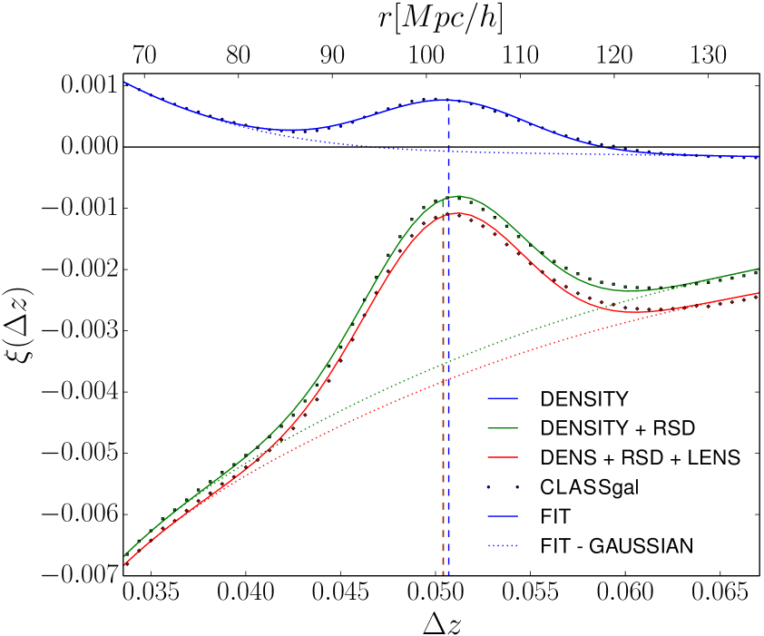
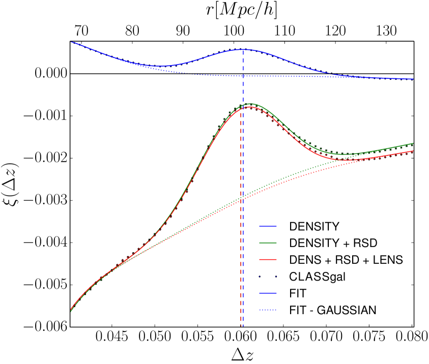
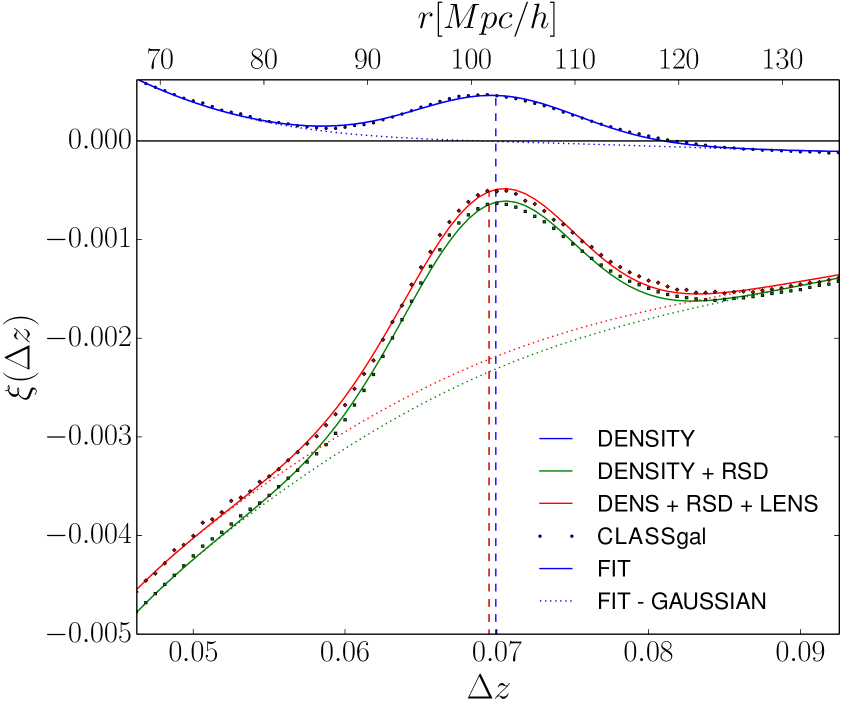
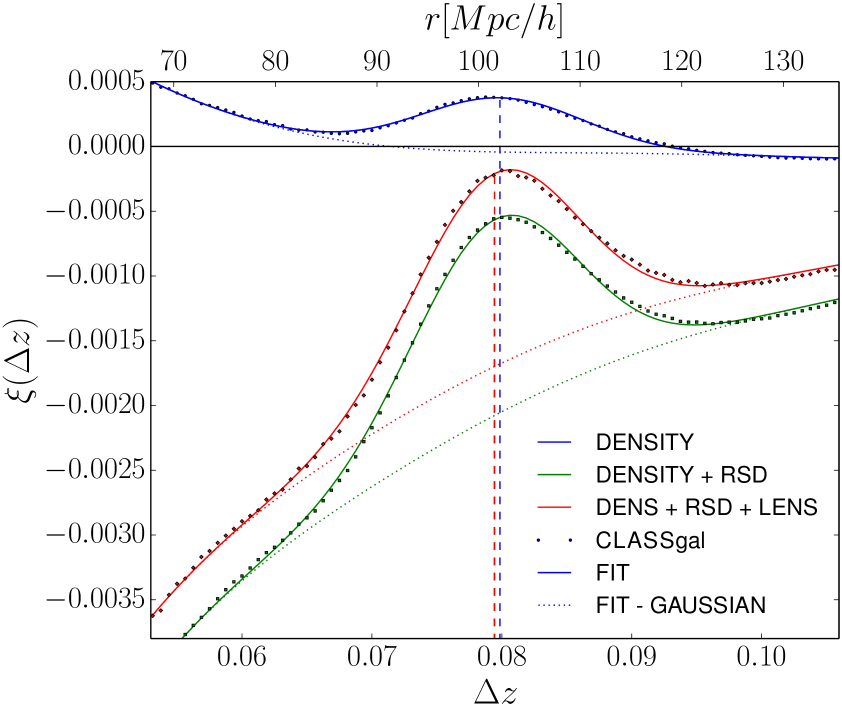
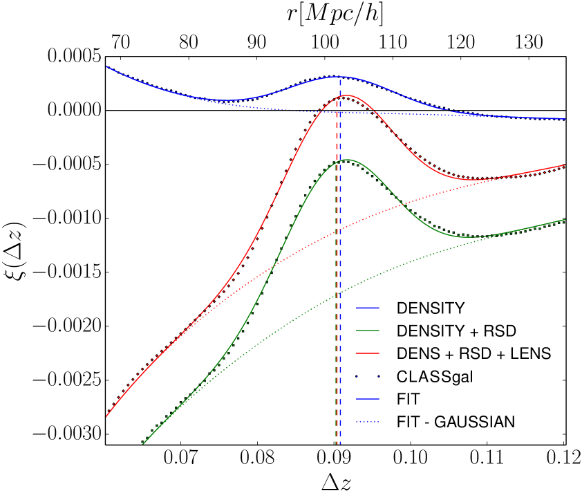
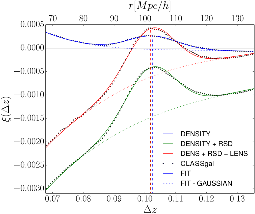
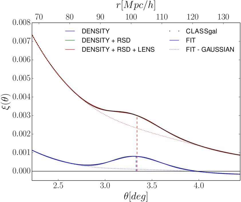
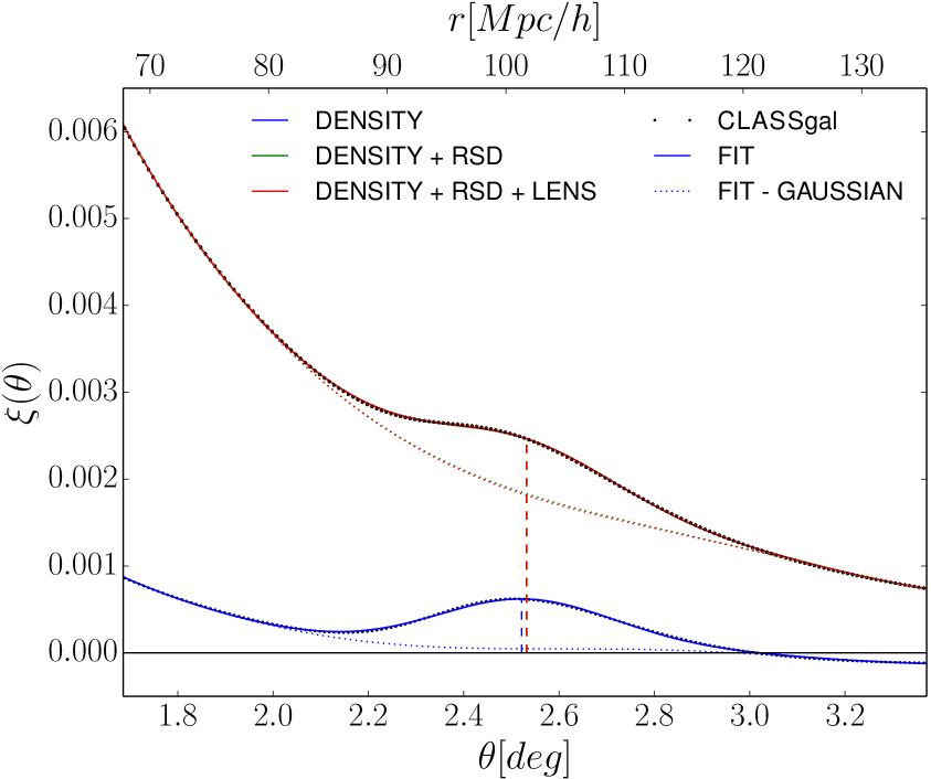
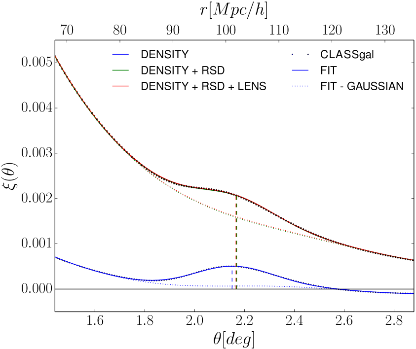
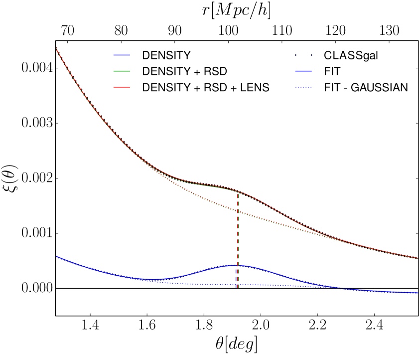
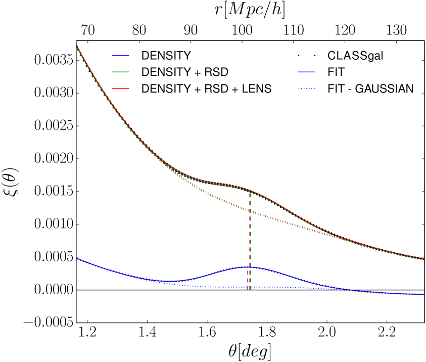
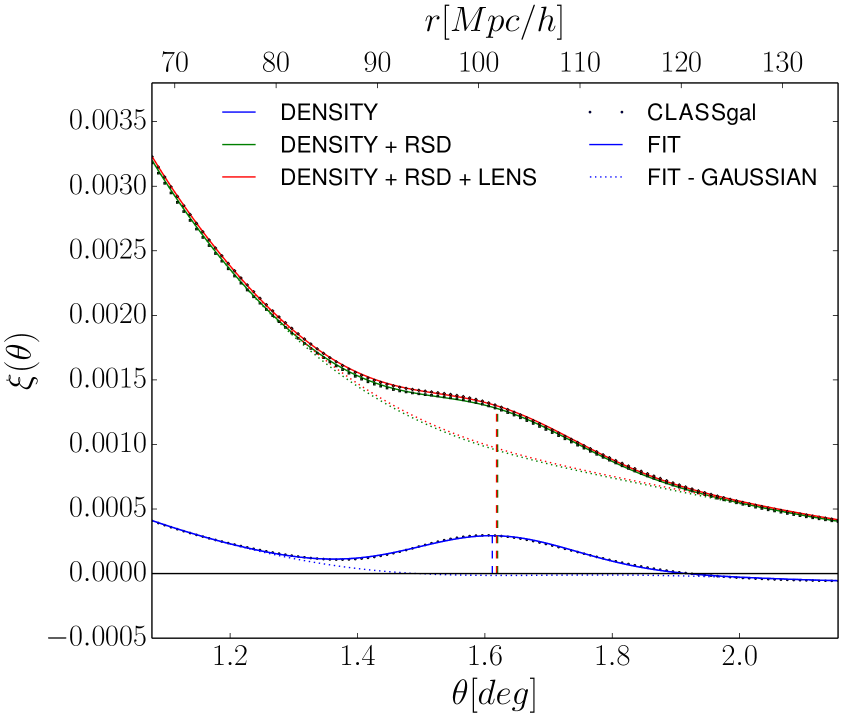
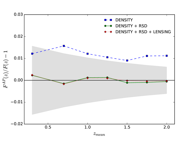
Figure 2 and Figure 3 show the radial and the transverse correlations and the corresponding fits for the three cases of interest, at different redshifts, respectively. As we have already seen in the previous sections, redshift space distortions significantly modify both the shape and the amplitude of the correlation functions in the radial and transverse directions. We remark that the ratio between the density and the redshift space distortions terms is only weakly sensitive to the mean redshift. Indeed, in linear theory only the growth factor has a weak redshift dependence. The estimated values of the position of the BAO peak are slightly affected in both directions: when we do not include RSD corrections the radial BAO peak is shifted toward larger scales, while the angular peak position $\theta_{\rm BAO}$ is shifted to smaller scales. Although both effects are small ($\sim$ 0.5%), they sum up when applied to the AP test. This result should not be interpreted as a physical shift of the acoustic scale, it is a numerical effect related to the model assumed for the numerical fit, which is calibrated to be valid in redshift space and not in real space.

Figure 4: AP consistency test for the three cases analysed in this section. The shaded region represents the expected errors around zero. The errors on $F_{\rm AP}$ are estimated from the propagation of uncertainties, see eq. (A.1) in Appendix A. Uncertainties on $\Delta z_{\rm BAO}$ and $\theta_{\rm BAO}$ are assumed to be due to the resolution of the survey: we set $\delta z=6.25\cdot 10^{-4}$; this is the resolution used to compute radial correlations, while for the angular resolution we assume the resolution of a Euclid-like survey, i.e. $\delta\theta_{\rm BAO}=0.1\,\mbox{arcsec}$. The error on $F_{\rm AP}$ results to be dominated by the uncertainty on $\Delta z_{BAO}$.

The gravitational lensing correction does not affect the transverse correlation function, while in the radial direction it changes the amplitude, but not the shape of the correlation function. Therefore, it does not appreciably shift the peak position. In Figure 2 we show that the lensing term reduces the amplitude of the radial correlation function at low redshifts, while it increases the amplitude at high redshifts. This is due to the fact that the lensing contribution is dominated by the negative correlation between density and lensing at low redshifts, while is dominated by the auto-correlation at high redshifts.

In Figure 4 we show the result of the consistency test for the three cases of interest here. We find that gravitational lensing does not affect the AP test, while redshift space distortions enhance the result by about 1% if compared to an analysis performed in real space.

5.2 Galaxy bias

In the previous section we assumed observed galaxies to be unbiased tracers of the underlying dark matter distribution. In this section we relax this assumption in order to investigate the implication of galaxy bias for the BAO measurements and for the AP test. The effect of galaxy bias on BAO measurement was investigated in [30], where it was found that for the most biased tracers ($b>3$) a non-linear shift on the acoustic scale occurred at the percent level. However, it has been demonstrated that applying BAO reconstruction [31] compensates for this effect.

In this work we aim to study how a simple local and linear bias model influences the AP test. In fact, the bias affects the computation of the correlation function, but does not enter in the theoretical value of the AP parameter. Hence, any deviation from the theoretical value, is due to our ability of determining the BAO scale in terms of the truly observable quantities $\xi_{\parallel}\left(\Delta z,z_{\text{mean}}\right)$ and $\xi_{\perp}\left(\theta,z_{\text{mean}}\right)$. Since in the previous section we have found that lensing does not affect the measurement of the AP parameter, we neglect the lensing contribution here. We follow an analogous procedure as in the previous section, but here we vary the bias parameter $b$, that we assume to be redshift and scale independent (this assumption can also be easily generalized).

Figure 5: AP consistency test for different values of the bias parameter $b$. The red line is computed including the only contribution from the local density field. The shaded region highlights the typical error-bars around zero. The most biased tracers cause an offset up to $1\%$. This systematic uncertainty should be taken into account in the total error budget.

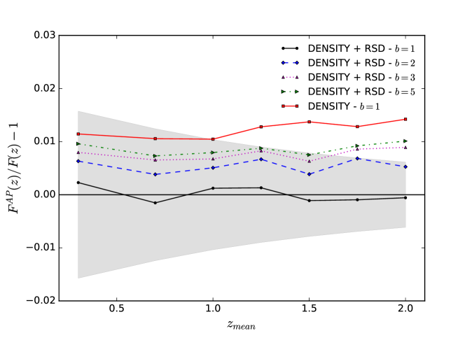
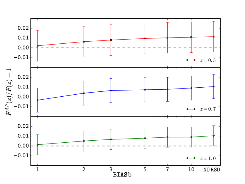
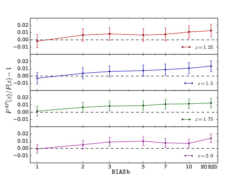
In Figure 5 we show the result of the AP consistency test for different values of the bias parameter. We see that the bias causes an offset which grows with increasing bias. This offset is due to the fact that the BAO position is recovered by using the phenomenological parameterization (4.3), which has been calibrated for unbiased sources. From Figs. 2 and 3 we note that the shape changes considerably when including redshift space distortions in the correlation function. Therefore, correlation functions for different galaxy bias parameters ($b>1$) range between the blue and the green lines in Figs. 2 and 3 and they affect the precision of the parameterization. This indicates, that even when working only with directly observable quantities, we need to assume some cosmological prior to be able to determine accurately the BAO position. Nevertheless, to perform an AP test we do not need to know the physical scale of BAO, and so we can use radial and transverse correlation functions to self-calibrate the parameterizations.

In Figure 6 we show how the offset varies as a function of the bias parameter, at fixed redshift. When increasing the bias, this offset approaches the offset found for an unbiased tracer, when only the local density term is taken into account. Indeed, for large galaxy bias parameters the redshift space distortions contribution tends to be negligible. As expected there is only a marginal redshift dependence, since we have considered a redshift independent bias and there is only a weak redshift dependence in the relation between the density and the velocity transfer functions, given by the growth factor. In a given survey, it is therefore important to reconstruct the bias as good as possible. In this way the fitting procedure can be calibrated for the estimated bias and the impact of the systematic error investigated in this section can be mitigated.

Figure 6: AP consistency test, at fixed redshift, for different values of the bias parameter.

5.3 The radial window function

In the previous section we assumed that the redshifts of the sources are exactly known. In realistic applications, though, a redshift bin has finite thickness that can be modeled by a window function (usually a Gaussian or a top-hat) centered at some mean redshift.

To be able to locate the radial BAO peak position a spectroscopic precision (typically $\sigma_{z}=0.001(1+z_{\text{mean}})$ or smaller) for the redshift determination is required, whereas photometric redshift resolution is not sufficient.

For this reason we will focus here on spectroscopic surveys.

However, in the transverse correlation function, the presence of a radial window function does not affect the resolution, but it smears out the BAO feature. As shown in Fig. 8, redshift bins of a typical width of photometric survey are sufficient to locate the peak position, but the position depends on the bin-width, see also [17].

Even if the AP test can be performed only with data from a spectroscopic survey, we can employ a window function with width larger than the redshift uncertainty in order to maximize the signal-to-noise ratio

$$\Biggl{(}\frac{S}{N}\Biggr{)}_{\theta}=\frac{\xi_{\perp}(\theta)}{\sigma_{\xi_{\theta}}},$$ (5.1)

where the noise $\sigma_{\xi_{\theta}}$ is given by the root mean square of the diagonal elements of the covariance matrix $\mathtt{COV}$

$$\mathtt{COV}_{\theta\theta^{\prime}}=\frac{2}{f_{\rm sky}}\sum_{\ell=0}^{\ell_{max}}\frac{2\ell+1}{(4\pi)^{2}}\Bigl{[}P_{\ell}(\cos{\theta})\Bigr{]}\Bigl{[}P_{\ell}(\cos{\theta^{\prime}})\Bigr{]}\Biggl{(}C_{\ell}+\frac{1}{n_{i}}\Biggr{)}^{2},$$ (5.2)

$$\sigma_{\xi_{\theta}}=(\mathtt{COV}_{\theta\theta})^{1/2}.$$ (5.3)

In the expression (5.2), $f_{\rm sky}$ is the fraction of the sky covered by the survey. The shot noise is computed as the inverse of the number of galaxies per steradian $n_{i}$ inside the $i$-th redshift bin.

In order to find the width of the window function which maximizes the signal-to-noise ratio, we compute this quantity for different values of $\sigma_{z}$

$$\sigma_{z}=\mathtt{w}\cdot(1+z_{\rm mean}),\qquad\mathtt{w}=0.005,0.01,0.02,0.03,$$ (5.4)

at different redshift in the range $z_{\rm mean}=[0.7-2.0]$ and for the different specifications of the survey. We consider three future planned galaxy redshift surveys: Euclid, the Square Kilometer Array (SKA) and the Dark Energy Spectroscopic Instrument (DESI). As for DESI, we consider the two classes of galaxies that will be targeted by this experiment: bright Emission Line Galaxies (ELGs), that will be observed up to $z=1.7$, and Luminous Red Galaxies (LRGs), that will be observed up to $z=1.0$.

In Appendix B we present the survey specifications we use in the computation of the signal-to-noise ratio.

(a) Transverse correlation function and noise.

(b) Signal-to-noise ratio.

Figure 7: In Figure 7(a) and Figure 7(b) we show, respectively, the transverse correlation function with its corresponding noise and the signal-to-noise ratio for different widths of the Gaussian window function. Both figures refer to the case of an Euclid-like survey at redshift $z=1$.

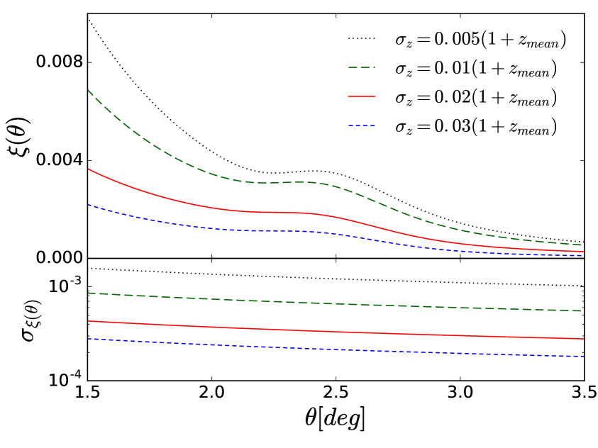
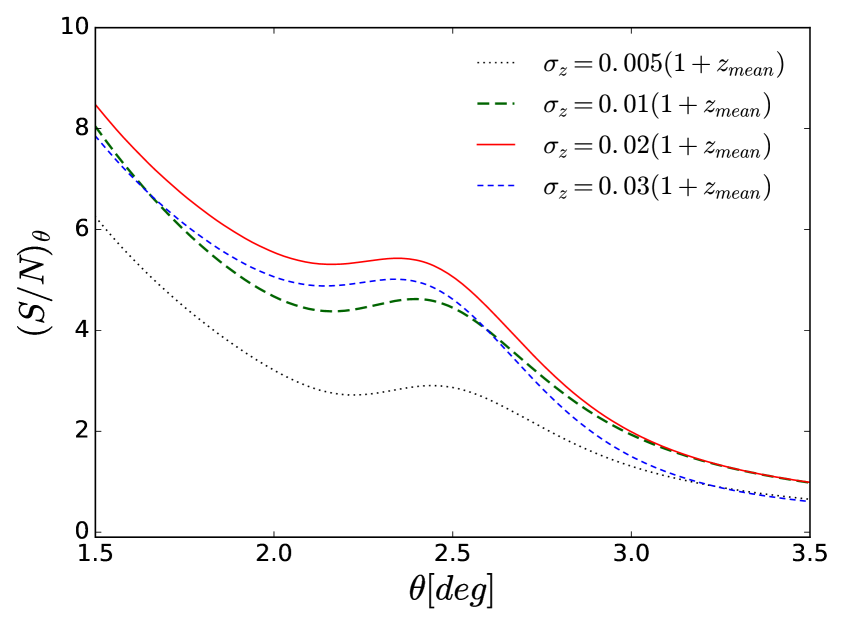
In Figure 7 we show, as an example, the comparison of the signal-to-noise ratio for a Euclid-like galaxy survey at redshift $z=1$. From Figure 7(a) we see that, for a large window function, the signal is suppressed, but the correspondent noise also decreases. We find that the signal-to-noise ratio, around the BAO peak, is optimized for $\sigma_{z}=0.02(1+z_{\rm mean})$ (Figure 7(b)). For all the four sets of survey specifications analyzed here, we find the same result. Therefore, from now on, we set our window function to $\sigma_{z}=0.02(1+z_{\rm mean})$.

Now we are interested in studying the effect of a window function on the transverse correlation function and thereby on the AP test.

Since we consider window function with width much larger than the redshift resolution, we assume a top-hat radial window in the transverse correlation function and we refer to $\sigma_{z}$ as the half-width of the top-hat.

In the radial correlation, a window with spectroscopic width ($\sigma_{z}=0.001(1+z_{\text{mean}})$ or smaller) does not substantially affect the correlation function because it still includes only radial modes. Therefore, we used a Delta Dirac window.

Figure 8: Transverse correlation function, at $z=1$, for different width of the window function. For the thick continuous lines only density and redshift space distortions are included, while in the thin dashed lines also the lensing term is taken into account.

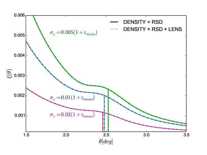
In Figure 8 we compare the transverse correlation function computed applying three window functions of different widths. In this example, we assume bias $b=1$ and, use the analytic expression from [32] for the galaxy density distribution,

$$\frac{dN}{dz}\propto\Biggl{(}\frac{z}{0.5}\Biggr{)}^{2}\exp{\Biggl{[}-\biggl{(}\frac{z}{0.5}\biggr{)}^{1.5}\Biggr{]}}.$$ (5.5)

The window function suppresses the correlations and it shifts the peak position toward smaller angular scales, which is in agreement with the result presented in [17]. Furthermore, we test the modifications induced by gravitational lensing in the transverse direction when a window function is employed. We find that gravitational lensing slightly modifies the amplitude of the correlation function, but this effect is negligible with respect to the suppression induced by the window and leaves the peak position unaffected.

In order to recover the physical BAO scale, the shift induced by the window function can be modeled as longitudinal component in the measured BAO scale. More precisely, the BAO scale can be computed as

$$L=\sqrt{L^{2}_{\perp}+\Biggl{(}\frac{\delta z}{H(z)}\Biggl{)}^{2}},$$ (5.6)

where $L_{\perp}$ is estimated from the BAO peak in transverse correlation function, while the corrective term $\delta z$ is a function of the width $\sigma_{z}$ of the window function. We use the parameterization introduced in [17], where the corrective term is simply proportional to $\sigma_{z}$

$$\delta z=\sqrt{\gamma}\sigma_{z}.$$ (5.7)

Here we predict the value of the corrective factor $\gamma$ from the AP test, for three future galaxy redshift surveys previously quoted: Euclid, SKA and DESI.

We introduce also a realistic model for the redshift dependence of galaxy bias.

We perform the AP test, by introducing the radial window in the transverse correlations and modeling a redshift dependent bias in both radial and transverse correlation functions.

For all four considered surveys, we find that the redshift binning generates an offset between $3\%$ and $5\%$ (see Figure 9, dash lines). Minor differences between the four cases are due to the different galaxy density distributions and the redshift dependence of the galaxy biases.

Figure 9: The result of the AP test for the four survey specifications considered. The dash lines refer to the cases in which a window function with $\sigma_{z}=0.02(1+z_{\rm mean})$ is used and no correction is applied in order to take into account the effect of the window function. The dotted lines refer to the case in which no window function is employed (the small deviations are due to the redshift dependent bias). The continuous lines represents the cases with window function in the radial direction and which are corrected using the expression (5.8), where $\gamma$ are the best-fit values, reported in Table 1.

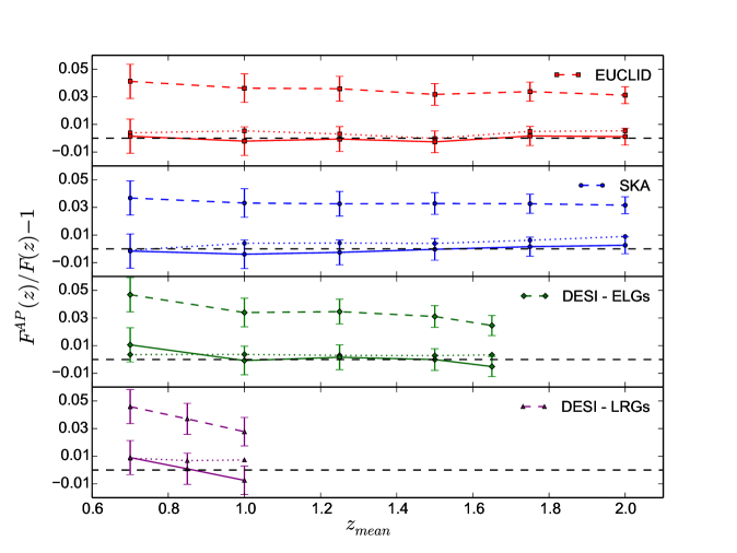
In order to correct the result of the test from the distortions induced by the window function, we model the true AP parameter, as follows from Eqs. (5.6, 5.7) and as already suggested in [17]

$$F_{\rm AP}(z_{\rm mean})=\frac{\Delta z_{\rm BAO}}{\theta_{\rm BAO}}\sqrt{1-\gamma\cdot\Biggl{(}\frac{\sigma_{z}}{\Delta z_{\rm BAO}}\Biggr{)}^{2}},$$ (5.8)

where $\gamma$ is the parameter which quantifies the offset due to the window function. We estimate the parameter $\gamma$ by minimizing the quantity

$$\chi^{2}=\sum_{i}\Biggl{(}\frac{F_{\rm AP}(z_{i})-F_{\rm th}(z_{i})}{\Delta F_{\rm AP}(z_{i})}\Biggr{)}^{2},$$ (5.9)

where $F_{\rm th}$ is the expected value for the AP function and $\Delta F_{\rm AP}$ is the error on $F_{\rm AP}$, determined by the redshift and angular uncertainties, which we assume to be statistically independent at different redshifts. The values of $\gamma$ which minimizes the difference between the measured AP function and its theoretical values are reported in Table 1.

In Figure 9 we show, as solid lines, the results of the test properly corrected for the window function effect. We find that, within the error, the AP function computed from angular and radial positions of the BAO peak in the correlation function agrees with the theoretical value.

	Bias	$\gamma$
Euclid-like	$\sqrt{1+z}$	0.166
SKA	$c_{4}\exp{(c_{5}z)}$	0.161
DESI - ELGs	$0.84/D(z)$	0.151
DESI - LRGs	$1.7/D(z)$	0.154

Table 1: Best-fit values of the parameter $\gamma$, for the four different survey specifications. The parameters which specify the bias dependence on redshift for SKA are taken from Table 4 in [33], telescope SKA (phase 2). The galaxy bias model for DESI depends on the linear growth factor $D(z)$.

5.4 Impact of shot-noise on the AP test

In the previous Section, we tested the precision of the AP test for different sources of uncertainties. In particular, in Section 5.2 we found that the galaxy bias introduces an extra 1% error in the estimation of $F_{\rm AP}$. In this Section we quantify the impact of the shot-noise in the computation of the peak position and on the AP function. We estimate the uncertainty on the cosmological parameters obtained from the AP test including shot-noise and cosmic variance in the error budget. Our estimate is approximate, the true errors are somewhat larger.

We consider an Euclid-like survey, with specifications as described in Appendix B. We first compute the errors induced by shot-noise and cosmic variance as the statistical 1-$\sigma$ errors on our fitting parameters for the correlation functions.

The error is computed in two steps. First, we include the error due to the shot-noise and cosmic variance in the fitting procedure by minimizing

$$\chi^{2}=\sum_{i}\Biggl{(}\frac{\xi(\theta_{i})-\hat{\xi}(\theta_{i},\mathbf{p})}{\sigma_{\xi_{\theta_{i}}}}\Biggr{)}^{2},$$ (5.10)

where $\hat{\xi}(\theta,\mathbf{p})$ is the parameterization described in Eq. (4.3), $\mathbf{p}$ is the vector of our fitting parameters and ${\bf\sigma}_{\xi_{\theta_{i}}}$ are the errors of the correlation function, defined in (5.3). Eq. (5.10) implicitly assumes the errors $\sigma_{\xi_{\theta_{i}}}$ to be uncorrelated, which is not true for the angular correlation function. Nevertheless, the correlations between errors do not affect the estimated values of the best-fit parameters, but only their covariance. For this reason, we compute the best-fit parameters by assuming eq. (5.10) and we separately estimate their errors. The errors on the parameters $\mathbf{p}$ are estimated as

$$\sigma_{\mathbf{p}}=\sqrt{\mbox{diag}([\mathbf{J^{T}WJ}]^{-1})},$$ (5.11)

where $\mathbf{J}$ is the Jacobian of the transformation

$$J^{ij}=\frac{\partial\hat{\xi}(\theta_{i},\mathbf{p})}{\partial p_{j}},$$ (5.12)

and $\mathbf{W}$ is the inverse of the full covariance matrix $\mathtt{COV}$,

$$W^{ij}=[\mathtt{COV}_{\theta^{i}\theta^{j}}]^{-1}.$$ (5.13)

The covariance matrix is computed from eq. (5.2).

We use a tophat window function of half-width $\sigma_{z}=0.02(1+z_{\rm mean})$, which maximizes the signal-to-noise ratio as shown in Section 5.3.

	$\sigma_{\theta_{\rm BAO}}$ [%]		$\sigma_{\theta_{\rm BAO}}$ [%]
	Cosmic variance + shot-noise		Cosmic variance
z	Polynomial	Power-law	Polynomial	Power-law
0.7	2%	1.4%	2%	1.4%
1.0	3%	1.9%	1.7%	1.0%
1.25	3%	1.9%	1.6%	0.9
1.5	3%	2.3%	1.5%	0.8
1.75	5%	3%	1.4%	0.9%
2.0	12%	8%	1.3%	0.7%

Table 2: 1-$\sigma$ statistical error on $\theta_{\rm BAO}$ estimated by the fit for two different parameterizations. The polynomial parameterization is the polynomial+Gaussian we adopted throughout the paper, where the polynomial degree is set to be $N=10$, while the power-law is the 6-parameter power-law+Gaussian model considered in Appendix A.

In Table 2 we report the errors on $\theta_{\rm BAO}$ computed at different redshifts for two different parameterizations. The polynomial model is the $10$ degrees polynomial+Gaussian we tested in the previous sections, see Eq. (4.3), which fits 14 parameters. The power-law+ Gaussian model refers the parameterization tested in Appendix A, see Eqs. (A.3, A.4), which is based on 6 parameters. In both cases, we find that the statistical errors dominate the uncertainties due to the angular resolution of the survey. At low redshift ($z<1.5$), the statistical error is dominated by cosmic variance, while shot-noise dominates at high redshifts ($z\geq 1.5$), where the error rapidly increases up to $\sim 10\%$ (see Table 2). Somewhat surprisingly, the errors for the power-law + Gaussian model are smaller than the ones estimated for the polynomial+Gaussian model, as shown in Table 2.

This suggests that a fitting model with 14 parameters, even if more accurate, requires more data to constrain simultaneously the free parameters and the cosmological model. Table  2 shows that a power-law still gives better constraints. Nevertheless, the power-law template may introduce a bias in the result, as it is shown in Appendix A. Therefore, it can be worth to partially sacrifice the precision of the result in favor of a better accuracy.

In order to estimate the impact of these errors on the AP function we compute the total error by summing the systematic errors, due to the resolution of the survey and on the bias, and the statistical errors, due to the shot-noise and cosmic variance,

$$\frac{\Delta F_{\rm AP}}{F_{\rm AP}}=\sqrt{\Biggl{(}\frac{\Delta F_{\rm AP}}{F_{\rm AP}}\Biggr{)}_{\rm sys}^{2}+\Biggl{(}\frac{\Delta F_{\rm AP}}{F_{\rm AP}}\Biggr{)}_{\rm stat}^{2}}.$$ (5.14)

Figure 10: Impact of shot-noise on the error of the AP function.

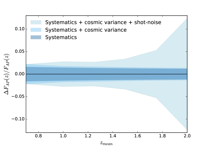
In Figure 10 we show the impact of the error due to the shot-noise on the AP function. When only the systematic error is taken into account, the error is dominated by the resolution in redshift in the radial correlation function. The shot-noise contribution is, however, not negligible and becomes even dominant at high redshifts, due to the lower galaxy density. This indicates that with a higher number of galaxies, one could improve the AP test significantly. If both sources of uncertainty are taken into account we find a relative error between 3% and 4% at $z\leq 1.5$, while at higher redshift the error increases up to 12% at $z=2$.

In the low redshift regime ($z\leq 1.5$), the estimated errors for the AP parameter $F_{\rm AP}$ can be compared to the recent analysis presented by the Baryon Oscillation Spectroscopic Survey (BOSS) collaboration [34]. In [34] the AP parameter is estimated in three redshift bins in the range $z\in[0.2,0.75]$ and in each bin the analysis uses the full two-dimensional correlation function. For all the three bins, the errors on $F_{\rm AP}$ amount approximatively to $3\%$ (see Table 4 in [34]), which is the same order of the errors in Figure 10 in the low redshift regime.

5.5 Constraints on cosmological parameters

To conclude, we give in this section an approximative estimation of the expected errors on $\Omega_{\rm m}$, $\Omega_{\rm k}$ and $w_{\rm DE}$ from the AP test.

First we study the dependence of the AP function on cosmological parameters. In Figure 11 we show the sensitivity of the AP function to variations of the cosmological parameters when considering BOSS error-bars from only galaxy clustering [35] (left panel), and the Planck 2015 error-bars [2](right panel).

(a) BOSS - Galaxy clustering only

(b) Planck 2015

Figure 11: Sensitivity of the AP function to different cosmological parameters. $\Delta\Omega_{i}$ is taken to be the error on the parameter $\Omega_{i}$ from galaxy clustering only (top panel) and from CMB analysis (bottom panel). The constraints from galaxy clustering come from the Baryon Oscillation Spectroscopic Survey (BOSS) of SDSS-III, when only the CMASS-Large dataset is employed [35]. The constraints from CMB are the 1-$\sigma$ limits ($\Omega_{\rm m}$) and 2-$\sigma$ limits ($\Omega_{\rm k}$ and $w_{\rm DE}$) in Planck 2015 analysis [2], when CMB plus external data are used. The sign change in $\frac{\partial F_{\rm AP}}{\partial w_{\rm DE}}$ at $z\simeq 1.3$ is well visible in the precise Planck data ’smeared out’ in the less accurate BOSS data.

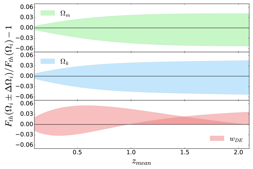
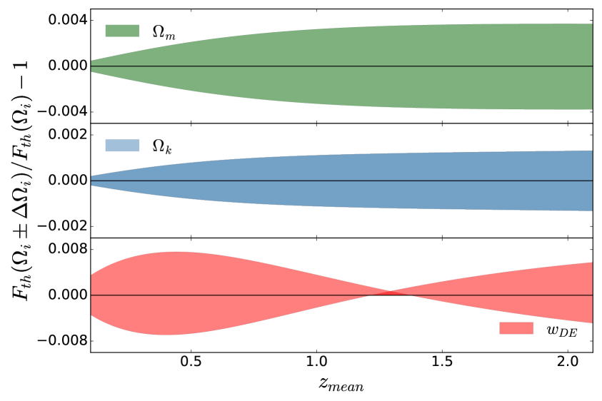
For each parameter, we also naively compute its change over the allowed range of variation of the AP function when all the other parameters are kept fixed,

$$\Delta\Omega_{i}(z)=\Biggl{(}\frac{\partial F_{\rm AP}}{\partial\Omega_{i}}\Biggr{)}^{-1}\Delta F_{\rm AP}.$$ (5.15)

We use for $\Delta F_{\rm AP}$ the error computed in Section 5.4 and plotted in Figure 10.

In Figure 12 we compare $\Delta\Omega_{i}(z)$ to the constraints presently available from galaxy clustering data, more precisely from BOSS [35], and from the state-of-the-art constraints, given by Planck, CMB + External Data analysis [2]. The errors $\Delta\Omega_{i}(z)$ are represented by the light shaded regions, while the errors from BOSS (only galaxy clustering) and Planck 2015 are shown in dotted and dashed line, respectively.

Figure 12: Constraints on cosmological parameters from a single measurement of the AP function (light shaded region) and from $N=14$ measurements (assumed to be independent) (dark shaded region). The Planck and BOSS limits are indicated by dashes and dotted horizontal lines.

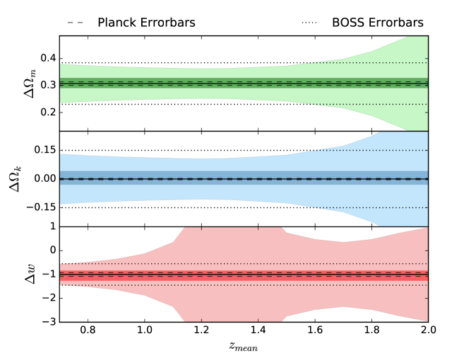
The equation of state of dark energy, for this simple parameterization, is poorly constrained in the AP test around $z\sim 1.3$. This reflects the fact that the AP parameter is not sensitive to $w$ around $z\sim 1.3$, as we see in Figure 11.

The light shaded regions in Figure 12 represent the error on a single measurement of $F_{\rm AP}$, the overall statistical errors on the parameters can be reduced by performing $N$ independent measurements at different redshifts.

We also estimate the errors from $N=14$ independent measurements in the range $[0.7,2.0]$ with redshift separation $\Delta z=0.1$. The errors are estimated by fitting a set of hypothetical data points for the AP function $F_{\rm DATA}$. The data points are computed by summing the value of $F_{\rm AP}$ for our fiducial cosmology to a randomly generated scattering term proportional to the error. The fit is performed by running $\mathtt{emcee}$ [36], a Markov Chain Monte Carlo (MCMC) code. The $\chi^{2}$ inferred from the simulated data is

$$\chi^{2}=\sum_{i=1}^{N}\Biggl{(}\frac{F_{\rm DATA}(z_{i})-F_{\rm AP}(z,\Omega)}{\Delta F_{\rm AP}}\Biggr{)}^{2},$$ (5.16)

where we vary only one parameter $\Omega$ at a time, keeping the others fixed to their fiducial value.

We obtain the following results for $\Omega_{m}$, $\Omega_{k}$ and $w_{\rm DE}$:

$$\Omega_{m}=0.309^{+0.019}_{-0.018},\qquad\Omega_{k}=0.005^{+0.036}_{-0.034},\qquad w_{\rm DE}=-1.02^{+0.18}_{-0.24},$$ (5.17)

where the quoted errors are the $1-$sigma limits.

The dark shaded regions in Fig. 12 shows the error regions given in (5.17). The error-bars from the AP test are still significantly larger than the Planck error bars but smaller that present errors obtained from galaxy clustering only.

The most recent analysis combining CMB data with BAO and redshift space distortions is presented by the BOSS collaboration [37]. The errorbars on the three cosmological parameters $\Omega_{m}$, $\Omega_{k}$ and $w_{\rm DE}$ are comparable to the Planck 2015 errorbars and therefore result to be significantly smaller than the errors quoted in (5.17). This is not surprising since the AP test uses just one single scale in the power spectrum, while parameter estimation from the full CMB power spectrum (Planck), or the full shape of the correlation function (BOSS), has the advantage of using all available modes.

6 Conclusions

We have presented a model independent method to perform the Alcock Paczyński test. We applied the test to the BAO feature in the galaxy 2-point correlation function, in the radial and transverse directions. In order to perform the test without prior assumption on the cosmological parameters, we model the shape of the correlation function with a polynomial, while the acoustic feature is modeled as a Gaussian. In this work we have shown that both redshift space distortions and galaxy bias must be taken into account to improve the accuracy of the estimated BAO scale, while gravitational lensing does not significantly affect the result of the AP test. Finally, we have investigated the projection effect induced by the finite width of the radial window function. In fact, in the transverse direction a redshift bin of a typical width of a photometric survey is sufficient to locate the peak position and it can be employed to maximize the signal-to-noise. However, the projection effect shifts the measured acoustic peak toward smaller angular scale. If not corrected for, this introduces a systematic error of up to $5\%$ in the AP test. We have computed the correction that has to be applied in order to adjust the result of the test for this effect for three planned galaxy surveys, Euclid-like, SKA and DESI. We have also estimated the effect of shot-noise and cosmic variance in the precision of the BAO peak detection and on the AP test. We have found that the precision of the test could be improved significantly by increasing the number of galaxies in the survey, especially at high redshift. Finally, we have shown that cosmological parameters can be estimated in a model independent approach, by the AP test, with roughly the same accuracy as the BAO analysis performed with the BOSS survey. The latter, however, has the disadvantage to use the power spectrum in Fourier space, $P(k)$, which itself depends in a non-trivial way on cosmological parameters via the conversion of angles and redshifts into distances.

Appendix A Methodology tests

Here we report the results of some tests we performed in order to find the best method to model the transversal and longitudinal correlation functions and in order to verify its reliability.

Figure 13: AP consistency test for different degrees $N$ of the polynomial in the parameterization of the correlation function. The error-bars are computed from linear propagation of uncertainty, eq. (A.1), assuming the uncertainty on $\Delta z_{BAO}$ and $\theta_{BAO}$ to be the resolution of the galaxy survey.

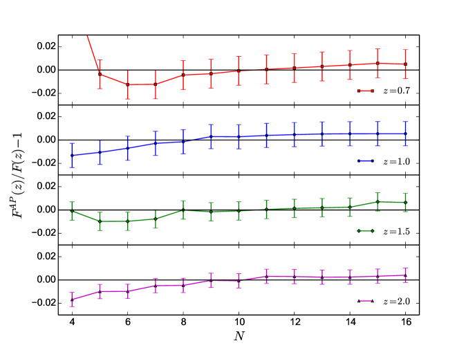
We test our template model, Eq. (4.3), for different degrees of the fitting polynomial. Figure 13 shows a consistency check for values of $N$ in the range $[4:16]$. The correlation functions used in this test are computed including the local density term and the redshift space distortions correction.

The errorbars are computed from linear propagation of uncertainty,

$$\frac{\Delta F_{\rm AP}}{F_{\rm AP}}=\sqrt{\Biggl{(}\frac{\delta z}{\Delta z_{\rm BAO}}\Biggr{)}^{2}+\Biggl{(}\frac{\delta\theta_{\rm BAO}}{\theta_{\rm BAO}}\Biggr{)}^{2}},$$ (A.1)

where $\delta z=6.25\cdot 10^{-4}$ is the resolution used for the radial correlation function, and $\delta\theta_{\rm BAO}=0.1$ arcsec is the angular resolution of an Euclid-like survey.

For these values, the uncertainty due to the angular resolution can be safely neglected and the relative error can be written as

$$\frac{\Delta F_{\rm AP}}{F_{\rm AP}}=\frac{\delta z}{\Delta z_{\rm BAO}}.$$ (A.2)

Since $\delta z$ is chosen to be constant, the errorbars decrease at larger redshift because the radial BAO peak position corresponds to larger $\Delta z_{\rm BAO}$.

We found that for $N$ between 8 and 14 the relative difference between the fitted AP parameter and its theoretical value is smaller than $0.5\%$ at all redshifts. We checked the accuracy of the fit comparing the sum of the squared deviations between our fit and the classgal output and we found the most numerically accurate results satisfying the AP test. Therefore, we choose a polynomial of degree $N=10$ to perform the next analysis. In order to test the goodness of this parameterization, we perform the same analysis for different cosmologies, including a cosmology with a dynamical dark energy equation of state. In all cases we find qualitatively the same behavior shown in Figure 13. We compare our parameterization also with others described in the literature. In particular, the transverse correlation function is often modeled by a power-law + Gaussian function [38]

$$\xi_{\perp}(\theta)=A+B\cdot\theta^{\gamma}+C\cdot e^{-(\theta-\theta_{\rm BAO})^{2}/2\sigma^{2}},$$ (A.3)

with $A$, $B$, $\gamma$, $C$, $\theta_{\rm BAO}$ and $\sigma$ as free parameters. As for the radial correlation function, we compare our model with the parameterization used in [39]

$$\xi_{\parallel}(\Delta z)=A+B\cdot e^{-C\Delta z}-D\cdot e^{-E\Delta z}+F\cdot e^{-(\Delta z-\Delta z_{\rm BAO})^{2}/2\sigma^{2}},$$ (A.4)

where the free parameters are $A$, $B$, $C$, $D$, $E$, $F$, $\Delta z_{\rm BAO}$ and $\sigma$. The result of this consistency test is shown in Figure 14. We find that both the exponential parameterization, Eq. (A.4), and the 10 degree polynomial, Eq. (4.3), fit well the radial correlation function (differences are smaller than 0.5% at all redshifts for the AP consistency check). On the other hand, we find a discrepancy between the power-law and the polynomial parameterization for the transverse correlation function.

Figure 14: AP consistency test at different redshifts, for different parameterization of the radial and transverse correlation functions. The continuous black line refers to the test performed using a polynomial fitting function for the estimation of both $\Delta z_{\rm BAO}$ and $\theta_{\rm BAO}$, the dot blue line is computed using a polynomial fit in the longitudinal direction and the power-law+Gaussian model in the transverse one, while the dash green line is computing using a polynomial for $\xi_{\perp}(\theta)$ and the exponential fit in (A.4) for $\xi_{\parallel}(\Delta z)$.

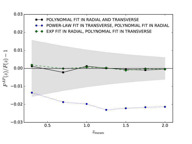
In Table 3 we compare the comoving BAO scale computed from the peak positions in the transverse and radial direction.

We find that, using a power-law+Gaussian fit for the transverse correlation function, the peak position is systematically shifted towards larger scales. This systematic introduces a 2% offset in the AP test.

The polynomial and the exponential parameterization gives consistent values of the BAO scale at all redshifts. However, the polynomial fit is able to model the data over a larger range, therefore we adopt this parameterization.

$z$	$L_{\perp}(Mpc/h)$		$L_{\parallel}(Mpc/h)$
	Polynomial	Power-law	Polynomial	Exponential
0.3	101.7 $\pm$ 0.2	103.2 $\pm$ 0.2	101.9 $\pm$ 1.6	102.0 $\pm$ 1.6
0.7	101.9 $\pm$ 0.3	103.6 $\pm$ 0.3	101.7 $\pm$ 1.3	101.9 $\pm$ 1.3
1.0	101.8 $\pm$ 0.4	103.9 $\pm$ 0.4	101.9 $\pm$ 1.1	101.8 $\pm$ 1.1
1.25	101.8 $\pm$ 0.5	104.3 $\pm$ 0.5	101.9 $\pm$ 0.9	101.9 $\pm$ 0.9
1.5	101.9 $\pm$ 0.5	104.1 $\pm$ 0.5	101.8 $\pm$ 0.8	101.8 $\pm$ 0.8
1.75	101.9 $\pm$ 0.6	104.0 $\pm$ 0.6	101.8 $\pm$ 0.7	101.8 $\pm$ 0.7
2.0	101.9 $\pm$ 0.6	104.0 $\pm$ 0.6	101.8 $\pm$ 0.6	101.8 $\pm$ 0.6

Table 3: The comoving BAO scale in units of Mpc$/h$ computed using the different parameterizations given in the text for the correlation function at different redshifts.

Appendix B Surveys specifications

In this section we report the specifications used for the different surveys considered in Section 5.3. The parameters of the surveys are the sky coverage $f_{\rm sky}$, the number of galaxies per unit redshift per square degree and the redshift dependence of the galaxy bias.

(a) Number of galaxies per square degree per unit redshift.

(b)
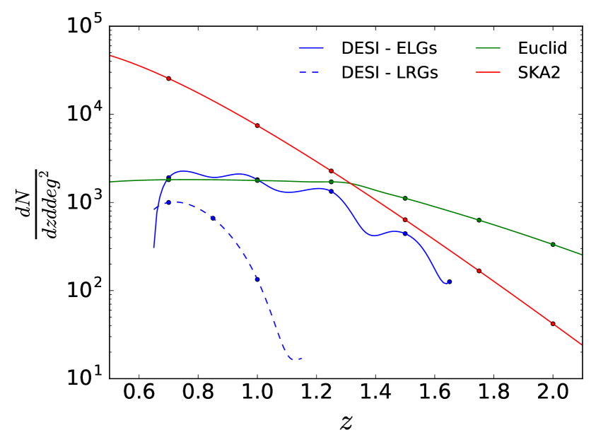
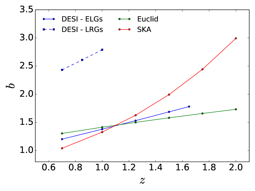
Redshift evolution of the galaxy bias.

Figure 15: Figure 15(a) and Figure 15(b) show, respectively, the number of galaxies per square degree per unit redshift and the redshift dependent bias for the four cases described in this Appendix: Euclid, SKA, DESI ELGs (bright Emission Line Galaxies) and DESI LRGs (Luminous Red Galaxies). The markers identify the redshifts for which we performed the AP test in Section 5.3.

B.1 Euclid

Our Euclid-like survey is modeled following Appendix A.3 in [40]. We assume a sky fraction $f_{\rm sky}=0.375$. The number of galaxies per unit redshift per square degree is computed from Table 2 of [41], for the case of a limiting flux of $3\times 10^{-16}\rm{erg}\,\rm{s}^{-1}\,\rm{cm}^{-2}$. Following Ref. [40], we multiply the tabulated values by an efficiency factor $0.25$ and we divide them by the factor $1.37$ to get conservative prediction. The redshift dependence of the bias is modeled as in the forecasts presented in [18]

$$b(z)=\sqrt{1+z}.$$ (B.1)

B.2 SKA

We used the technical specification for SKA reported in [20]. Galaxy number density per unit redshift per square degree and bias evolution are given by

$$\frac{dN}{dzd\Omega} =10^{c_{1}}z^{c_{2}}\exp{(-c_{3}z)},$$ (B.2)

$$b(z) =c_{4}\exp{(c_{5}z)},$$ (B.3)

where we used for the coefficients $c_{i}$ the best-fit values reported in Table 4 of [33], for SKA2. For SKA2, the sky coverage is expected to be around $30000\,\mbox{deg}^{2}$, which corresponds to a sky fraction $f_{\rm sky}=0.727$.

B.3 DESI

Survey specifications for DESI, for both ELGs and LRGs, are taken from the Science Technical Design Report [42]. The number of galaxies per unit redshift per square degree, for both ELGs and LRGs, are assumed to be the one reported in Table 2.3 of [42]. The values at intermediate redshifts are computed by interpolation. The redshift dependence of galaxy bias is expressed in terms of the linear growth factor $D(z)$. For the ELGs we have

$$b(z)=\frac{0.84}{D(z)},$$ (B.4)

while for LRGs we assume

$$b(z)=\frac{1.7}{D(z)}.$$ (B.5)

Following [42], we assume for DESI a sky coverage equal to $14000\,\mbox{deg}^{2}$, which corresponds to a sky fraction $f_{\rm sky}=0.339$. In Figure 15 we compare the expected number of galaxies per unit redshift, per square degree and the bias evolution for the 3 cases discussed above. The number of galaxies per unit redshift per square degree is relevant for the computation of shot noise.

The number of galaxies per steradian $n_{i}$ inside the $i$-th redshift bin is computed as

$$n_{i}=\frac{1}{4\pi}\int d\Omega\int_{z_{\rm mean}-\Delta z/2}^{z_{\rm mean}+\Delta z/2}\frac{dN}{dzd\Omega}dz,$$ (B.6)

where $\Delta z$ is the width of the redshift bin.

References

- [1] WMAP Collaboration, G. Hinshaw et al., Nine-Year Wilkinson Microwave Anisotropy Probe (WMAP) Observations: Cosmological Parameter Results, Astrophys. J. Suppl. 208 (2013) 19, [arXiv:1212.5226].
- [2] Planck Collaboration, P. A. R. Ade et al., Planck 2015 results. XIII. Cosmological parameters, arXiv:1502.01589.
- [3] D. H. Weinberg, M. J. Mortonson, D. J. Eisenstein, C. Hirata, A. G. Riess, and E. Rozo, Observational Probes of Cosmic Acceleration, Phys. Rept. 530 (2013) 87–255, [arXiv:1201.2434].
- [4] S. Weinberg, The cosmological constant problem, Rev. Mod. Phys. 61 (Jan, 1989) 1–23.
- [5] J. Frieman, M. Turner, and D. Huterer, Dark Energy and the Accelerating Universe, Ann. Rev. Astron. Astrophys. 46 (2008) 385–432, [arXiv:0803.0982].
- [6] R. Durrer and R. Maartens, Dark Energy and Dark Gravity, Gen. Rel. Grav. 40 (2008) 301–328, [arXiv:0711.0077].
- [7] J. Yoo, A. L. Fitzpatrick, and M. Zaldarriaga, New perspective on galaxy clustering as a cosmological probe: General relativistic effects, Physical Review D 80 (Oct., 2009) 083514, [arXiv:0907.0707].
- [8] J. Yoo, General relativistic description of the observed galaxy power spectrum: Do we understand what we measure?, Physical Review D 82 (Oct., 2010) 083508, [arXiv:1009.3021].
- [9] C. Bonvin and R. Durrer, What galaxy surveys really measure, Phys. Rev. D84 (2011) 063505, [arXiv:1105.5280].
- [10] A. Challinor and A. Lewis, The linear power spectrum of observed source number counts, Phys. Rev. D84 (2011) 043516, [arXiv:1105.5292].
- [11] J. Yoo and M. Zaldarriaga, Beyond the Linear-Order Relativistic Effect in Galaxy Clustering: Second-Order Gauge-Invariant Formalism, Phys. Rev. D90 (2014), no. 2 023513, [arXiv:1406.4140].
- [12] D. Bertacca, R. Maartens, and C. Clarkson, Observed galaxy number counts on the lightcone up to second order: I. Main result, JCAP 1409 (2014), no. 09 037, [arXiv:1405.4403].
- [13] E. Di Dio, R. Durrer, G. Marozzi, and F. Montanari, Galaxy number counts to second order and their bispectrum, JCAP 1412 (2014) 017, [arXiv:1407.0376]. [Erratum: JCAP1506,no.06,E01(2015)].
- [14] N. Kaiser, Clustering in real space and in redshift space, Monthly Notices of the Royal Astronomical Society 227 (July, 1987).
- [15] W. Cardona, R. Durrer, M. Kunz, and F. Montanari, Lensing convergence in galaxy redshift surveys, arXiv:1603.06481.
- [16] C. Alcock and B. Paczynski, An evolution free test for non-zero cosmological constant, Nature 281 (Oct, 1979).
- [17] F. Montanari and R. Durrer, A new method for the Alcock-Paczynski test, Phys. Rev. D86 (2012) 063503, [arXiv:1206.3545].
- [18] Euclid Theory Working Group Collaboration, L. Amendola et al., Cosmology and fundamental physics with the Euclid satellite, Living Rev. Rel. 16 (2013) 6, [arXiv:1206.1225].
- [19] DESI Collaboration, M. Levi et al., The DESI Experiment, a whitepaper for Snowmass 2013, arXiv:1308.0847.
- [20] Cosmology SWG Collaboration, F. B. Abdalla et al., Cosmology from HI galaxy surveys with the SKA, arXiv:1501.04035.
- [21] E. Di Dio, F. Montanari, R. Durrer, and J. Lesgourgues, Cosmological Parameter Estimation with Large Scale Structure Observations, JCAP 1401 (2014) 042, [arXiv:1308.6186].
- [22] É. Aubourg et al., Cosmological implications of baryon acoustic oscillation measurements, Phys. Rev. D92 (2015), no. 12 123516, [arXiv:1411.1074].
- [23] E. Di Dio, F. Montanari, J. Lesgourgues, and R. Durrer, The CLASSgal code for Relativistic Cosmological Large Scale Structure, JCAP 1311 (2013) 044, [arXiv:1307.1459].
- [24] J. Lesgourgues, The Cosmic Linear Anisotropy Solving System (CLASS) I: Overview, ArXiv e-prints (Apr., 2011) [arXiv:1104.2932].
- [25] D. Blas, J. Lesgourgues, and T. Tram, The Cosmic Linear Anisotropy Solving System (CLASS) II: Approximation schemes, JCAP 1107 (2011) 034, [arXiv:1104.2933].
- [26] T. Matsubara, The Correlation function in redshift space: General formula with wide angle effects and cosmological distortions, Astrophys. J. 535 (2000) 1, [astro-ph/9908056].
- [27] T. Matsubara, Correlation function in deep redshift space as a cosmological probe, Astrophys. J. 615 (2004) 573–585, [astro-ph/0408349].
- [28] “MPFIT python version.” http://cars9.uchicago.edu/software/python/mpfit.html.
- [29] J. J. Moré, Numerical Analysis: Proceedings of the Biennial Conference Held at Dundee, June 28–July 1, 1977, ch. The Levenberg-Marquardt algorithm: Implementation and theory, pp. 105–116. Springer Berlin Heidelberg, Berlin, Heidelberg, 1978.
- [30] K. T. Mehta, H.-J. Seo, J. Eckel, D. J. Eisenstein, M. Metchnik, P. Pinto, and X. Xu, Galaxy Bias and its Effects on the Baryon Acoustic Oscillations Measurements, Astrophys. J. 734 (2011) 94, [arXiv:1104.1178].
- [31] D. J. Eisenstein, H.-j. Seo, E. Sirko, and D. Spergel, Improving Cosmological Distance Measurements by Reconstruction of the Baryon Acoustic Peak, Astrophys. J. 664 (2007) 675–679, [astro-ph/0604362].
- [32] M. Crocce, A. Cabre, and E. Gaztanaga, Modeling the angular correlation function and its full covariance in Photometric Galaxy Surveys, Mon. Not. Roy. Astron. Soc. 414 (2011) 329–349, [arXiv:1004.4640].
- [33] M. G. Santos, D. Alonso, P. Bull, M. Silva, and S. Yahya, HI galaxy simulations for the SKA: number counts and bias, arXiv:1501.03990.
- [34] BOSS Collaboration, A. G. Sanchez et al., The clustering of galaxies in the completed SDSS-III Baryon Oscillation Spectroscopic Survey: cosmological implications of the configuration-space clustering wedges, Submitted to: Mon. Not. Roy. Astron. Soc. (2016) [arXiv:1607.03147].
- [35] C.-H. Chuang et al., The clustering of galaxies in the SDSS-III Baryon Oscillation Spectroscopic Survey: single-probe measurements from CMASS and LOWZ anisotropic galaxy clustering, arXiv:1312.4889.
- [36] D. Foreman-Mackey, D. W. Hogg, D. Lang, and J. Goodman, emcee: The MCMC Hammer, Publ. Astron. Soc. Pac. 125 (2013) 306–312, [arXiv:1202.3665].
- [37] BOSS Collaboration, S. Alam et al., The clustering of galaxies in the completed SDSS-III Baryon Oscillation Spectroscopic Survey: cosmological analysis of the DR12 galaxy sample, Submitted to: Mon. Not. Roy. Astron. Soc. (2016) [arXiv:1607.03155].
- [38] E. Sanchez, A. Carnero, J. Garcia-Bellido, E. Gaztanaga, F. de Simoni, M. Crocce, A. Cabre, P. Fosalba, and D. Alonso, Tracing The Sound Horizon Scale With Photometric Redshift Surveys, Mon. Not. Roy. Astron. Soc. 411 (2011) 277–288, [arXiv:1006.3226].
- [39] E. Sanchez, D. Alonso, F. J. Sanchez, J. Garcia-Bellido, and I. Sevilla, Precise Measurement of the Radial Baryon Acoustic Oscillation Scales in Galaxy Redshift Surveys, Mon. Not. Roy. Astron. Soc. 434 (2013) 2008–2019, [arXiv:1210.6446].
- [40] B. Audren, J. Lesgourgues, S. Bird, M. G. Haehnelt, and M. Viel, Neutrino masses and cosmological parameters from a Euclid-like survey: Markov Chain Monte Carlo forecasts including theoretical errors, JCAP 1301 (2013) 026, [arXiv:1210.2194].
- [41] J. E. Geach et al., Empirical H-alpha emitter count predictions for dark energy surveys, Mon. Not. Roy. Astron. Soc. 402 (2010) 1330, [arXiv:0911.0686].
- [42] DESI Collaboration, Desi technical design report part i: Science,targeting, and survey design, 2015.