Ising Spin Glasses in dimension five

Abstract

Ising spin glass models with bimodal, Gaussian, uniform and Laplacian interaction distributions in dimension five are studied through detailed numerical simulations. The data are analyzed in both the finite-size scaling regime and the thermodynamic limit regime. It is shown that the values of critical exponents and of dimensionless observables at criticality are model dependent. Models in a single universality class have identical values for each of these critical parameters, so Ising spin glass models in dimension five with different interaction distributions each lie in different universality classes. This result confirms conclusions drawn from measurements in dimension four and dimension two.

I Introduction

The statistical physics of second order transitions has been intensively studied in standard systems exemplified by pure ferromagents, and a thorough understanding of the critical behavior has been reached based on Renormalization Group Theory (RGT). RGT provides an elegant explanation of the universality of critical exponents, which is the property that all systems within the same universality class (determined only by the physical dimension $d$ and the spin dimension $N$) have identical values for each critical exponent and for characteristic dimensionless critical parameters. It has been implicitly or explicitly assumed that in spin glasses the form of the interaction distribution is not a relevant parameter for the determination of the universality class, so that in particular all Ising Spin Glasses (ISGs) in a given dimension are expected to have the same critical exponents and critical parameters. The ISG situation is in fact much less clear cut; it has been stated that a fundamentally different theoretical approach to transitions is required parisi:01 ; castellana:11 ; angelini:13 . We have found from numerical studies on Ising spin glasses (ISGs) in dimensions $4$ and $2$ having bimodal and Gaussian interaction distributions lundow:15 ; lundow:15a ; lundow:16 that the critical exponents and the critical values for dimensionless constants are not identical for the two models in a given dimension but that they vary with the interaction distribution. It was concluded that the universality class of an ISG depends not only on the physical dimension of the system but also on the form of the interaction distribution.

Here numerical simulation data on ISGs in dimension $5$ are presented and analysed. We are aware of no analogous simulation measurements on ISGs in dimension $5$, but some of the present measurements can be compared to results on the same models obtained from the High Temperature Series Expansion (HTSE) technique klein:91 ; daboul:04 . Again, as in dimensions $4$ and $2$ the values for critical dimensionless constants and for the critical exponents are found to vary with the form of the interaction distribution, confirming that the non-universality conclusion reached for ISGs can be generalized.

Dimension $5$ is close to the ISG upper critical dimension $d=6$. For reference, the $\epsilon$-expansion ISG exponent values to leading order in $\epsilon=6-d$ gardner:84 are $\gamma=1+(6-d)$, $\nu=1/2+5(6-d)/12$ and $\eta=-(6-d)/3$, so for dimension $5$ the leading order exponent values are $\gamma=2$, $\nu=11/12\approx 0.92$, and $\eta=-1/3\approx-0.33$. The terms of higher order in $\epsilon$ are strong and no summations over all terms are known. There are no interaction distribution dependent terms in the standard $\epsilon$-expansion expressions. The leading order $\epsilon$-expansion exponent values are all in rough agreement with but are about $25\%$ stronger than the range of numerical estimates for the 5D ISG exponents given below in the Conclusion, Table I, where for instance the $\gamma$ estimates run from $1.73(2)$ for the bimodal interaction model to $1.49(2)$ for the Laplacian interaction model.

II Historical note

In $1894$ Van der Waals introduced the concept of critical exponents, in the context of transitions in liquids; he derived values for the exponents in terms of what is now called a mean field theory vanderwaals:94 . His student Verschaffelt made very precise experimental measurements on capillarity, and in $1900$ published experimental estimates for the exponents which were not equal to the mean field values verschaffelt:00 . His results were ignored for sixty years because they had no theoretical support (see Ref. levelt:76 for an excellent historical account). The situation only changed with Onsager’s analytic proof of non-mean field exponent values in the $2$D Ising model onsager:44 , which finally led on to the establishment of the principle of universality, within the RGT concept wilson:71 .

Verschaffelt employed temperature dependent effective exponents in his analyses. Effective exponent analyses were re-introduced much later for experimental kouvel:64 and numerical orkoulas:00 ; butera:02 ferromagnetic data. Below we also will use effective exponents in the analysis of ISG simulation data. We obtain results which are firmly established empirically but for which a theoretical explanation is for the moment lacking.

III Simulation measurements

We are aware of no previous publications of precise simulation data on ISGs in dimension $5$. The standard ISG Hamiltonian is

$$\mathcal{H}=-\sum_{ij}J_{ij}S_{i}S_{j}$$ (1)

with the near neighbor symmetric distributions normalized to $\langle J_{ij}^{2}\rangle=1$. The normalized inverse temperature is $\beta=(\langle J_{ij}^{2}\rangle/T^{2})^{1/2}$. The Ising spins live on simple hyper-cubic lattices with periodic boundary conditions. The spin overlap parameter is defined as usual by

$$q=\frac{1}{L^{d}}\sum_{i}S^{A}_{i}S^{B}_{i}$$ (2)

where A and B indicate two copies of the same system. We have studied the symmetric bimodal ($\pm J$), Gaussian, uniform ($P(J)=1/[2\cdot 3^{1/2}]$ for $-3^{1/2}<J<3^{1/2}$) and Laplacian $P(J)=2^{1/2}\exp(-2^{1/2}|J|)$ distribution ISG models in dimension $5$.

The simulations were carried out using the exchange Monte-Carlo method for equilibration using so called multi-spin coding, on $2^{12}$ individual samples at each size from $L=3$ to $L=10$ for the bimodal and Gaussian models. (It can be noted that an $L=10$ sample in $d=5$ contains more spins than an $L=46$ sample in $d=3$, so the simulations are laborious. However, see the Thermodynamic Limit (ThL) figure of merit discussion in Section VI. For the uniform distribution model $2^{12}$ samples were studied up to $L=6$, and $2^{9}$ samples up to $L=9$, and for the Laplacian model $2^{12}$ samples were studied up to $L=6$ and $2^{9}$ samples up to $L=8$. An exchange was attempted after every sweep with a success rate of at least $30\%$. At least $40$ temperatures were used forming a geometric progression reaching up to $\beta_{\max}=0.42$ in the bimodal model, $\beta_{\max}=0.45$ in the Gaussian model, $\beta_{\max}=0.45$ in the uniform model and $\beta_{\max}=0.45$ in the Laplacian model. This ensures that our data span the critical temperature region which is essential for the finite-size scaling (FSS) analyses. Near the critical temperature the $\beta$ step length was at most $0.003$. The various systems were deemed to have reached equilibrium when the sample average susceptibility for the lowest temperature showed no trend between runs. For example, for $L=10$ this means about $200000$ sweep-exchange steps.

After equilibration, at least $200000$ measurements were made for each sample for all sizes, taking place after every sweep-exchange step. Data were registered for the energy $E(\beta,L)$, the correlation length $\xi(\beta,L)$, for the spin overlap moments $\langle|q|\rangle$, $\langle q^{2}\rangle$, $\langle|q|^{3}\rangle$, $\langle q^{4}\rangle$ and the corresponding link overlap $q_{\ell}$ moments. In addition the correlations $\langle E(\beta,L),U(\beta,L)\rangle$ between the energy and observables $U(\beta,L)$ were also registered so that thermodynamic derivatives could be evaluated using the thermodynamic relation $\partial U(\beta,L)/\partial\beta=\langle U(\beta,L),E(\beta,L)\rangle-\langle U(\beta,L)\rangle\langle E(\beta,L)\rangle$ where $E(\beta,L)$ is the energy ferrenberg:91 . Bootstrap analyses of the errors in the derivatives as well as in the observables $U(\beta,L)$ themselves were carried out. We follow the same analysis strategy for the 5D ISGs as for the $4$D ISGs lundow:14 ; lundow:15a .

IV Finite size scaling

The usual approach to critical parameter measurements through simulations is to study the size dependence of dimensionless observables $Q(\beta,L)$ (generally the Binder cumulant $g(\beta,L)=(3-\langle q^{4}\rangle/\langle q^{2}\rangle^{2})/2$ and the normalized correlation length $\xi(\beta,L)/L$) in the regime very near the critical point. $g(\beta,L)$ must saturate at $g(\beta,L)=1$ for $\beta\gg\beta_{c}$ which is not the case for $\xi(\beta,L)/L$. It can be noted that we find critical $g(\beta_{c})$ values much lower in 5D ISGs than in $3$D or even in $4$D ISGs, so the 5D $g(\beta,L)$ data have space to ”fan out” beyond $\beta_{c}$ making this parameter more efficient for critical regime analyses in 5D than in the other dimensions. The typical FSS expression, valid in the near critical region if there is a single dominant scaling correction term, is :

$$Q(\beta,L)=Q_{c}+AL^{-\omega}+B(\beta-\beta_{c})L^{1/\nu}$$ (3)

where $\nu$ is the correlation length critical exponent and $\omega$ is the exponent of the leading finite size correction term. For any dimensionless parameter $Q$ the $Q_{c}$ critical values are identical for all systems within a universality class. From the HTSE and thermodynamic limit (ThL) data which we will discuss later the 5D correction exponent is typically $\omega\approx 1.0$ in the different models.

We will use the finite size scaling measurements as one method to estimate the critical inverse temperatures $\beta_{c}$, together with the dimensionless parameter values $Q_{c}$ at criticality extrapolated to the infinite size limit. The critical exponent $\nu$ can be estimated from the derivatives at criticality through

$$\frac{\partial Q(\beta,L)}{\partial\beta}\Big{|}_{\beta_{c}}=A_{Q}L^{1/\nu}\left(1+a_{Q}L^{-\omega}+\cdots\right)$$ (4)

The critical exponent $\eta$ can be estimated through

$$\frac{\chi(\beta_{c},L)}{L^{2}}=A_{\chi}L^{-\eta}\left(1+a_{\chi}L^{-\omega}+\cdots\right)$$ (5)

For the present analysis we have recorded the FSS behavior of various dimensionless parameters in addition to the Binder cumulant $g(\beta,L)$ and the correlation length ratio $\xi(\beta,L)/L$. The dimensionless parameter $W(\beta,L)$ for Ising ferromagnets was introduced in Ref. lundow:10 . In the ISG context the parameter $W_{q}(\beta,L)$ is defined by

$$W_{q}(\beta,L)=\frac{1}{\pi-2}\left(\frac{\pi\,[\langle|q|\rangle]^{2}}{[\langle q^{2}\rangle]}-2\right)$$ (6)

In the same spirit we will also make use of other dimensionless parameters

$$h(\beta,L)=\frac{1}{\sqrt{\pi}-\sqrt{8}}\left(\sqrt{\pi}\,\frac{[\langle|q^{3}|\rangle]}{[\langle q^{2}\rangle]^{3/2}}-\sqrt{8}\right)$$ (7)

$$P_{W}=\left[\frac{\langle|q|\rangle^{2}}{\langle q^{2}\rangle}\right]$$ (8)

and the skewness

$$P_{\mathrm{skew}}=\left[\frac{\langle|q|^{3}\rangle}{\langle q^{2}\rangle^{3/2}}\right]$$ (9)

which also have analogous scaling properties.

V Thermodynamic derivative peak analysis

The thermodynamic derivative peak analysis can also be an efficient method for analyzing data in a ferromagnet or an ISG. Near criticality in a ferromagnet, for a number of standard observables $Q$ the heights of the peaks of the thermodynamic derivatives $\partial Q(\beta,L)/\partial\beta$ scale for large $L$ as ferrenberg:91 ; weigel:09

$$D_{\max}(L)=\frac{\partial Q(\beta,L)}{\partial\beta}\Big{|}_{\max}\propto L^{1/\nu}\left(1+aL^{-\omega/\nu}\right)$$ (10)

The observables used for $Q(\beta,L)$ can be for instance the Binder cumulant $g(\beta,L)$ or the logarithm of the finite size susceptibility $\ln(\chi(\beta,L))$ ferrenberg:91 . Without needing a value of $\beta_{c}$ as input, the large $L$ peak height $D_{\max}(L)$ against $L$ plot provides $1/\nu$ directly, to within scaling corrections.

In addition, the temperature location of the derivative peak $\beta_{\max}(L)$ scales as

$$\beta_{c}-\beta_{\max}(L)\propto L^{-1/\nu}\left(1+bL^{-\omega/\nu}\right)$$ (11)

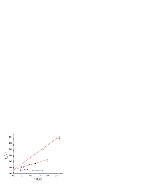
We note that the inverse of the derivative peak height $1/D_{\max}(L)$ and the peak location temperature difference $[\beta_{c}-\beta_{\max}(L)]$ are both proportional to $L^{-1/\nu}(1+aL^{-\theta/\nu}+\cdots)$ (with the leading correction terms having different pre-factors). Then $\beta_{\max}(L)$ plotted against $1/D_{\max}(L)$ must tend linearly towards the intercept $\beta_{c}$ as $1/D_{\max}(L)$ tends to zero for large $L$. All plots of the same type for different observables $Q$ should extrapolate consistently to the true $\beta_{c}$. The leading correction is eliminated to first order and together with the higher order corrections only appears as a modification to the straight line for small $L$. Provided that the peaks for the chosen observable fall reasonably close to $\beta_{c}$ these data can be much simpler to analyse than those from the crossing technique. For ferromagnets, Ferrenberg and Landau ferrenberg:91 found this form of analysis significantly more accurate than the standard Binder cumulant crossing approach.

In the ISG context exactly the same methodology can be used as in the ferromagnet lundow:15 . Because the exponent $\nu$ is relatively small in 5D ISGs this technique is an efficient independent method for estimating $\beta_{c}$. As far as we are aware this analysis has not been used previously by other authors in ISGs.

VI Thermodynamic limit scaling

The high temperature series expansion for the spin glass susceptibility of an ISG with a symmetrical interaction distribution can be written daboul:04

$$\chi(\beta^{2})=1+a_{1}\beta^{2}+a_{2}\beta^{4}+\cdots$$ (12)

Only even terms in powers of $\beta$ exist because of the symmetry between positive and negative interactions so $\beta^{2}$ rather than $\beta$ is the natural thermal scaling variable singh:86 ; klein:91 ; daboul:04 ; campbell:06 . (An equivalent natural scaling variable which has been generally used for HTSE analyses on ISGs with symmetric bimodal interaction distributions is singh:86 ; klein:91 $w=1-\tanh(\beta)^{2}/\tanh(\beta_{c})^{2}$. The discussion above holds throughout with $w$ replacing $\tau$. The exponents of course remain the same though the factors $C,a$ etc. are modified.) In principle an infinite set of exact HTSE factors $a_{n}$ exist. In practice terms in different ISG models have been calculated at best up to $n=15$ (see Refs. singh:86 ; klein:91 ; daboul:04 ). Then according to Darboux’s first theorem darboux:78 the asymptotic form of the sum of the entire series (all terms to infinite $n$) is eventually dominated by the closest singularity to the origin, which in the simplest case is the physical singularity, so near $\beta_{c}^{2}$

$$\chi(\beta^{2})=C_{\chi}\left[1-(\beta/\beta_{c})^{2}\right]^{-\gamma}$$ (13)

with $\beta_{c}^{2}$ being the inverse critical temperature squared and $\gamma$ the standard critical exponent.

It is thus natural to adopt $\tau=1-(\beta/\beta_{c})^{2}$ as the scaling variable in analyses of ThL ISG simulation data just as in the HTSE analysesdaboul:04 ; campbell:06 . Then the Wegner scaling expression wegner:72 for the ThL ISG susceptibility is

$$\chi(\tau)=C_{\chi}\tau^{-\gamma}\left(1+a_{\chi}\tau^{\theta}+b_{\chi}\tau^{\theta}{{}^{\prime}}+\cdots\right)$$ (14)

where $\theta=\nu\omega$ is the leading thermal correction exponent and the second term is generally analytic. The standard RGT scaling variable $t=(T-T_{c})/T_{c}$ is often used for ISG simulation analyses close to criticality, but this scaling variable is not convenient at higher temperatures as $t$ diverges at infinite temperature while $\tau$ tends to $1$. Also the temperature appears as $T$ not $T^{2}$ so $t$ is only appropriate for ISGs as an approximation near $\beta_{c}$.

The HTSE second moment of the ISG spin-spin correlations $\mu_{2}=\sum r^{2}\langle S_{0}.S{r}\rangle$ is of the form (see Ref. butera:02 ; campbell:08 for the ferromagnetic case)

$$\mu_{2}(\beta^{2})=\beta^{2}\left(z+b_{1}\beta^{2}+b_{2}\beta^{4}+\cdots\right)$$ (15)

where $z$ is the number of near neighbors. The ThL $\mu_{2}$ diverges at $\beta_{c}$ as $\tau^{-(\gamma+2\nu)}$. Then, invoking again Darboux’s theorem to link the series within the brackets to the critical divergence, the appropriate scaling form can be written as

$$\mu_{2}(\beta^{2})=C_{\mu}z\beta^{2}\tau^{-(\gamma+2\nu)}\left(1+a_{\mu}\tau^{\theta}+\cdots\right)$$ (16)

As the ThL second moment correlation length is defined through $\mu_{2}=z\chi(\beta)\xi(\beta)^{2}$, the Wegner form for the normalized ISG ThL correlation length can be written campbell:06

$$\xi(\beta)/\beta=C_{\xi}\tau^{-\nu}\left(1+a_{\xi}\tau^{\theta}+b_{\xi}\tau+\cdots\right)$$ (17)

It is important to note the factor $\beta$ which normalizes $\xi(\beta)$ in this equation.

The form of susceptibility scaling outlined here for ISGs was used from the earliest HTSE studies of critical behavior in ferromagnets and then in ISGs Refs. fisher:67 ; butera:02 ; klein:91 ; daboul:04 . The analogous normalized correlation length form was introduced explicitly in Ref. campbell:06 .

The full HTSE sum is by construction in the (infinite $L$) Thermodynamic limit (ThL) but extrapolations from high temperature must be made in order to estimate behavior at criticality, because the complete series is not available daboul:04 . Simulation data are necessarily taken at finite $L$, but can be considered as also being in the ThL as long as $L\gg\xi(\beta)$ where $\xi(\beta)$ is the ThL correlation length. The ThL envelope curves can generally be recognized by inspection of the data plots. As a rule of thumb, the condition $L>6\xi(\beta)$ can generally be taken as sufficient, with observables independent of $L$ and equal to the ThL values as long as this condition is satisfied. The simulation data supplement and extend the HTSE data. As $\xi(\beta)\sim\beta[1-(\beta/\beta_{c})^{2}]^{-\nu}$ in ISGs the ThL condition can be written approximately in terms of a figure of merit; if $\tau_{\min}$ is the lowest reduced temperature to which the ThL condition holds for size $L$,

$$\tau_{\min}\approx(L/6\beta_{c})^{-1/\nu}$$ (18)

In dimension $5$ with $\beta_{c}\approx 0.4$ and $\nu\approx 0.7$ the condition implies $\tau_{\min}\approx 0.15$ if the largest size used is $L=10$. This $\tau_{\min}$ corresponds to a temperature within $8\%$ of the critical temperature. It can be underlined that in dimension $3$ with the appropriate parameters for ISGs, $\beta_{c}\approx 1$, $\nu\approx 2.5$, to reach $\tau_{\min}\approx 0.15$ would require sample sizes to $L\approx 300$, far beyond the maximum sizes which have been studied numerically up to now in 3D ISGs. The ISG ThL regime can be studied numerically reasonably close to criticality in dimension $5$ (and dimension $4$) but the situation is much more delicate in dimension $3$.

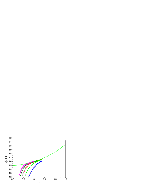
Temperature and size dependent susceptibility and correlation length effective exponents, valid over the entire paramagnetic regime, can be defined by

$$\gamma(\tau,L)=-\partial\ln\chi(\tau,L)/\partial\ln\tau$$ (19)

and

$$\nu(\tau,L)=-\partial\ln[\xi(\tau,L)/\beta]/\partial\ln\tau$$ (20)

The critical limits are $\gamma(0,\infty)=\gamma$ and $\nu(0,\infty)=\nu$; extrapolations must be made to estimate the critical exponents from HTSE or simulation data. In simple hyper-cubic lattices of dimension $d$ where $z=2d$ the exact ISG high temperature limits for all $L$ are $\gamma(1,L)=2d\beta_{c}^{2}$, and $\nu(1,L)=(d-K/3)\beta_{c}^{2}$ where $K$ is the kurtosis of the interaction distribution ($K=1$ for the bimodal distribution, $K=3$ for the Gaussian distribution, $K=9/5$ for the uniform distribution, and $K=6$ for the Laplacian distribution).

The value of $\beta_{c}$ enters implicitly into the definitions of $\gamma(\tau,L)$ and $\nu(\tau,L)$ in Eq. 19 and Eq. 20 through the definition of $\tau$, so it is important to have well established estimates for $\beta_{c}$ for the $\gamma$ and $\nu$ effective exponent analyses.

Turning to the exponent $\eta$, the temperature dependent effective $\eta(\beta,L)$ can be estimated through

$$2-\eta(\beta,L)=\frac{\partial\ln\chi(\beta,L)}{\partial\ln[\xi(\beta,L)/\beta]}=\frac{\gamma(\beta,L)}{\nu(\beta,L)}$$ (21)

Alternatively one can make a log-log plot of $y(\beta,L)=\chi(\beta^{2},L)/[\xi(\beta^{2},L)/\beta]^{2}$ against $x(\beta,L)=\xi(\beta^{2},L)/\beta$. At high temperatures and for all $L$, $x(\beta,L)$ and $y(\beta,L)$ both tend to $1$ as $\beta$ tends to $0$. For large $L$ and temperatures near criticality the slope of the ThL envelope curve $\partial\ln y(\beta,L)/\partial\ln x(\beta,L)$ tends to the critical exponent $-\eta$ in the limit $\beta\to\beta_{c}$ where both $y(\beta,L)$ and $x(\beta,L)$ diverge. With an appropriate fit function, extrapolation of the ThL envelope curve to the large $L$ limit leads to an estimate for $\eta$ purely from ThL data, without invoking the FSS estimate for $\beta_{c}$.

VII Privman-Fisher scaling

The Privman-Fisher scaling ansatz privman:84 for an observable $Q(\beta,L)$ can be written in the simple general form

$$Q(\beta,L)/Q(\beta,\infty)=F[L/\xi(\beta,\infty)]$$ (22)

where Wegner thermal correction terms are implicitly included in $Q(\beta,\infty)$ and $\xi(\beta,\infty)$. A leading finite size correction term can be introduced calabrese:03 :

$$\frac{Q(\beta,L)}{Q(\beta,\infty)}=F\left[L/\xi(\beta,\infty)\right]\left(1+\frac{G_{Q}\left[L/\xi(\beta,\infty)\right]}{L^{\omega}}\right)$$ (23)

For given values of the critical inverse temperature and exponents $\beta_{c}$, $\nu$ and $\eta$, assuming the leading ThL ISG extended scaling expressions $\chi(\beta,\infty)\propto[1-(\beta/\beta_{c})^{2}]^{-\gamma}$ and $\xi(\beta,\infty)\propto\beta[1-(\beta/\beta_{c})^{2}]^{-\nu}$ are valid and ignoring Wegner correction terms, the basic Privman-Fisher ansatz for the susceptibility can be readily transformed into

$$\frac{\chi(\beta,L)}{(L/\beta)^{2-\eta}}=\mathcal{F}[|(1-(\beta/\beta_{c})^{2})|(L/\beta)^{1/\nu}]$$ (24)

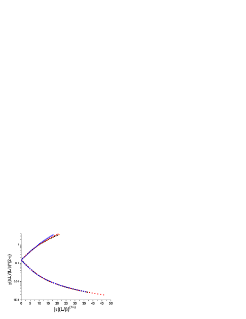
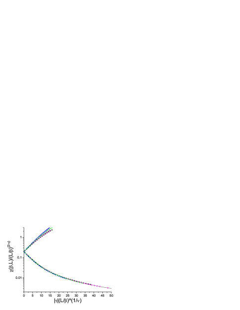
as applied in campbell:06 ; hukushima:09 . This extended scaling form is less sensitive to the precise values of the critical parameters than is the ThL scaling and does not contain the correction terms. However it allows one to scale all the data, not only those from the ThL regime, but also from the crossover regime between the ThL and FSS regimes, from the critical regime, and even from the region to temperatures rather below the critical temperature. Below it will be seen that very acceptable scaling is observed for the data from each of the four models studied, when the appropriate scaling parameters are used. This shows that the data for all $L$ and for all temperatures from infinity down to below $T_{c}$ can be encapsulated in the scaling expression (24), adjusting only the three critical parameters $\beta_{c}$, $\nu$ and $\eta$. If Wegner correction terms have been estimated from ThL scaling these can be introduced to improve the scaling but their influence will only be felt well outside the critical region.

VIII The 5D Gaussian distribution ISG model

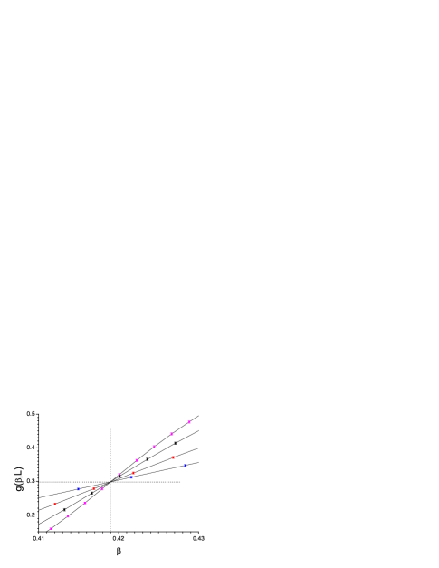
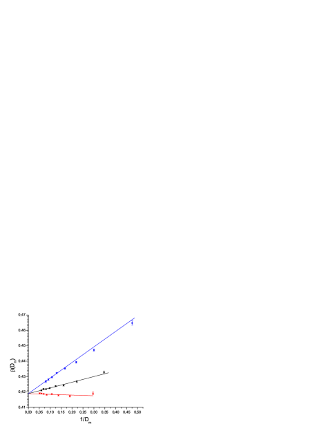
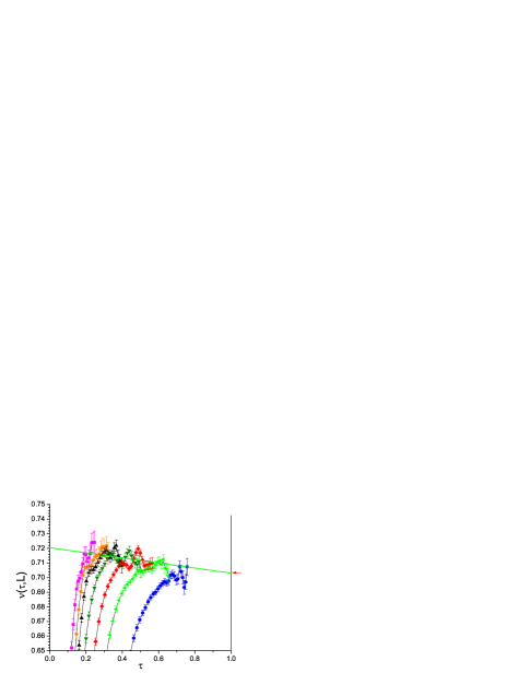
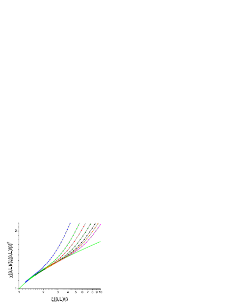
For the Gaussian distribution model, the FSS Binder parameter $g(\beta,L)$ data and the parameter $h(\beta,L)$ both happen to show no visible correction to scaling at criticality, Figs. 1 and 2. This provides us with consistent and accurate estimates $\beta_{c}=0.4190(3)$, $g_{c}=0.300(2)$ and $h_{c}=0.225(1)$. The data for the other dimensionless parameters in the form of fixed temperature plots show only weak corrections to scaling. They are all consistent with $\beta{c}=0.419$ and $\omega\approx 1$. As the finite size corrections are weak the analyses are rather insensitive to the assumed value for $\omega$, see for instance Fig. 3. The critical value estimates for the dimensionless parameters are listed in the Conclusion, Table I. Data for the locations of thermodynamic derivative peaks are shown in Fig. 4. They are also all consistent with $\beta_{c}=0.419$.

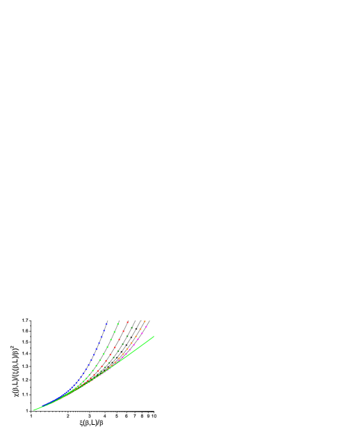
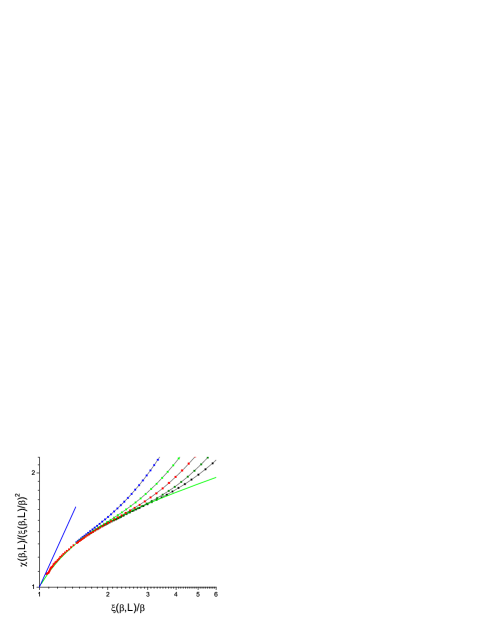
The effective exponents $\gamma(\tau,L)=\partial\ln\chi(\tau,L)/\partial\ln\tau$ and $\nu(\tau,L)=\partial\ln[\xi(\tau/L)/\beta]/\partial\ln\tau$ with $\beta_{c}$ fixed at $0.419$ are shown in Figs. 5 and 6. For Fig. 5 a HTSE curve (calculated with $a_{n}$ values obtained explicitly from summing the tabulation in daboul:04 ) is also included with the simulation data. This curve, calculated with the known $13$ leading HTSE terms only, is essentially exact in the high to moderate $\tau$ region. The numerical data are in excellent agreement with the HTSE curve. The fits to the ThL envelope data correspond to

$$\chi(\tau)=0.94\tau^{-1.59}\left(1+0.0625\tau^{2.4}\right)$$ (25)

and

$$\xi(\tau)=0.98\beta\tau^{-0.72}\left(1+0.017\tau^{2.4}\right)$$ (26)

Thus the exponent estimates are $\gamma=1.59(2)$ and $\nu=0.72(1)$ so $\eta=2-\gamma/\nu=-0.20(2)$. In Section XII a detailed discussion is given of the Gaussian HTSE estimates of Ref. daboul:04 . For both $\gamma$ and $\nu$ the corrections to scaling in the whole paramagnetic temperature region are weak. For $\chi(\tau)$ the ”effective” correction appears to be a sum of high-order correction terms. Any correction with $\theta\approx 1$, which might be expected from either the conformal correction or from a leading analytic correction, seems to be negligible.

A log-log plot of $y(\beta,L)=\chi(\beta^{2},L)/[\xi(\beta^{2},L)/\beta]^{2}$ against $x(\beta,L)=\xi(\beta^{2},L)/\beta$ is shown in Fig. 7. The estimated asymptotic slope of the ThL envelope curve $\partial\ln y(\beta,L)/\partial\ln x(\beta,L)$ gives an estimate for the critical exponent $\eta=-0.19(2)$ without invoking any value for $\beta_{c}$. This $\eta$ estimate is consistent with the value from the ratio $\gamma/\nu$.

The basic Privman-Fisher extended scaling (24) for $\chi(\beta,L)$ with these parameter values is shown in Fig. 8. The scaling is excellent (including the range of temperatures below $T_{c}$, the upper branch) apart from weak deviations visible for the smallest size $L=4$ which could be accounted for by a finite size correction term.

Figure 1: (Color on line) Gaussian 5D ISG model. Even $L$ Binder cumulants $g(\beta,L)$ against inverse temperature $\beta$, $L=4$, $6$, $8$ and $10$ (top to bottom on the left).

Figure 2: (Color on line) Gaussian 5D ISG model. Even $L$ data for the observable $h(\beta,L)$ against $\beta$, $L=4$, $6$, $8$ and $10$ (top to bottom on the left).

Figure 3: (Color on line) Gaussian 5D ISG. $P_{\mathrm{skew}}(\beta,L)$ against $1/L$ for fixed $\beta$, $\beta=0.424$, $0.422$, $0.420$, $0.419$, $0.418$, $0.416$ and $0.414$ (top to bottom). Dashed line : estimated criticality.

Figure 4: (Color on line) Gaussian 5D ISG. Peak location $y=\beta_{m}$ against inverse peak height $x=1/D_{m}$ for the derivatives $\partial P_{W}/\partial\beta$, $\partial h/\partial\beta$ and $\partial g/\partial\beta$ (top to bottom). Sizes $L=3$, $4$, $5$, $6$, $7$, $8$, $9$ and $10$ (increasing to the left). For each observable the points extrapolate to $y(x)=\beta_{c}$ at the lintercept, see text.

Figure 5: (Color on line) Gaussian 5D ISG. Effective exponent $\gamma(\tau,L)$ as function of $\tau$ with $\beta_{c}=0.419$. Points : simulation data for $L=10$, $9$, $8$, $7$, $6$, $5$ and $4$ (left to right). Dashed curve: fit. Continuous (green) curve on the right : calculated by summing the HTSE tabulation of daboul:04 .

Figure 6: (Color on line) Gaussian 5D ISG. Effective exponent $\nu(\tau,L)$ as function of $\tau$ with $\beta_{c}=0.419$. Points : simulation data for $L=10$, $9$, $8$, $7$, $6$, $5$ and $4$ (left to right). Continuous (green) curve : fit.

Figure 7: (Color on line) Gaussian 5D ISG. The ratio $\chi(\beta,L)/[\xi(\beta,L)/\beta]^{2}$ against $\xi(\beta,L)/\beta$ for $L=10$, $9$, $8$, $7$, $6$, $5$ and $4$ (right to left), continuous green curve : fit. No value is assumed for $\beta_{c}$.

Figure 8: (Color on line) Gaussian 5D ISG. Privman-Fisher-like scaling of the $\chi(\beta,L)$ data following the form used in campbell:06 , with assumed parameters $\beta_{c}=0.419$, $\nu=0.72$, $\eta=-0.19$ and no adjustments. $L=10$ pink squares, $L=8$ black circles, $L=6$ red triangles, $L=4$ blue inverted triangles. Upper branch : $\beta>\beta_{c}$, lower branch $\beta<\beta_{c}$.

IX The 5D bimodal distribution ISG model

For this model the dimensionless observable sets all show corrections to finite size scaling. Data for two typical observables are shown in Figs. 9 and 10. For $\beta_{c}$ the best overall estimate is $\beta_{c}=0.3885(5)$. Thermodynamic derivative peak location data are shown in Fig. 11. The extrapolations are consistent with the same value, $\beta_{c}=0.3885(5)$.

The effective exponents $\gamma(\tau,L)$ and $\nu(\tau,L)$ defined above are shown in Fig. 12 and 13. The high temperature curve included in Fig. 12 is evaluated from the HTSE series tabulation in Ref. daboul:04 . The critical exponents estimated by extrapolation are $\gamma=1.73(3)$ and $\nu=0.76(1)$, and the fit curves correspond to the ThL expressions

$$\chi(\tau)=0.73\tau^{-1.73}\left(1+0.37\tau^{0.95}-0.005\tau^{8}\right)$$ (27)

and

$$\xi(\tau)=0.94\beta\tau^{-0.76}\left(1+0.068\tau\right)$$ (28)

The simulation $\beta_{c}$, $\gamma$ and $\nu$ values are in excellent agreement with the quite independent HTSE bimodal critical value estimates $\beta_{c}=0.389(1)$, $\gamma=1.73(3)$, and $\nu\approx 0.73$ of Klein et al klein:91 discussed in detail in Section XII.

A log-log plot of $y(\beta,L)=\chi(\beta^{2},L)/[\xi(\beta^{2},L)/\beta]^{2}$ against $x(\beta,L)=\xi(\beta^{2},L)/\beta$ is shown in Fig. 14. The estimated limiting slope of the ThL envelope curve $\partial\ln y(\beta,L)/\partial\ln x(\beta,L)$ gives an estimate for the critical exponent $-\eta=0.28(1)$ without invoking any estimate for $\beta_{c}$. The Privman-Fisher extended scaling plot for $\chi(\beta,L)$ with these critical parameters is shown in Fig. 15.

Figure 9: (Color on line) Bimodal 5D ISG. $\xi(\beta,L)/L$ against $1/L$ for fixed $\beta$, $\beta=0.395$, $0.392$, $0.390$, $0.389$, $0.388$, $0.387$, $0.385$ and $0.382$ (top to bottom). $L=10$, $9$, $8$, $7$, $6$, $5$, $4$ and $3$ (right to left). Dashed line : estimated criticality, $\beta=0.3885$.

Figure 10: (Color on line) Bimodal 5D ISG. $P_{W}(\beta,L)$ against $1/L$ for fixed $\beta$, $\beta=0.385$, $0.387$, $0.388$ , $0.389$, $0.390$ and $0.392$ (top to bottom). $L=10$, $9$, $8$, $7$, $6$, $5$, $4$ and $3$ (left to right). Dashed line : estimated criticality, $\beta=0.3885$.

Figure 11: (Color on line) Bimodal 5D ISG. Peak location $y=\beta_{m}$ against inverse peak height $x=1/D_{m}$ for the derivative sets $\partial h(\beta,L)/\partial\beta$, $\partial P_{W}(\beta,L)/\partial\beta$, $\partial P_{\mathrm{skew}}(\beta,L)/\partial\beta$ and $\partial g(\beta,L)/\partial\beta$ (top to bottom). Sizes $L=3$, $4$, $5$, $6$, $7$, $8$, $9$ and $10$ (increasing to the left). For each observable the points extrapolate to $y(x)=\beta_{c}$ at the intercept, see text

Figure 12: (Color on line) Bimodal 5D ISG. Effective exponent $\gamma(\tau,L)$ as function of $\tau$ with $\beta_{c}=0.3885$. Points : simulation data for $L=10$, $9$, $8$, $7$, $6$, $5$ (left to right), continuous (blue) curve on the right : calculated by summing the HTSE tabulation of daboul:04 . Dashed line : fit.

Figure 13: (Color on line) Bimodal $5d$ ISG. Effective exponent $\nu(\tau,L)$ as function of $\tau$ with $\beta_{c}=0.3885$. Points : simulation data for for $L=10$, $9$, $8$, $7$, $6$ and $5$ (left to right). Red arrow : exact limit. Dashed line : fit

.

Figure 14: (Color on line) Bimodal 5D ISG. The ratio $\chi(\beta,L)/[\xi(\beta,L)/\beta]^{2}$ against $\xi(\beta,L)/\beta$ for $L=10$, $9$, $8$, $7$, $6$, $5$ and $4$ (right to left), continuous (green) curve : fit. No value is assumed for $\beta_{c}$.

Figure 15: (Color on line) Bimodal $5d$ ISG. Privman-Fisher-like scaling of the $\chi(\beta,L)$ data following the form used in campbell:06 , with assumed parameters $\beta_{c}=0.3885$, $\nu=0.77$, $\eta=-0.25$ and no adjustments. $L=10$ pink squares, $L=8$ black circles, $L=6$ red triangles, $L=4$ blue inverted triangles. Upper branch : $\beta>\beta_{c}$, lower branch $\beta<\beta_{c}$.

X The 5D uniform distribution ISG model

The numerical data for the uniform distribution model and the Laplacian distribution model are less complete than for the bimodal and Gaussian models. Nevertheless reliable critical parameter estimates have been obtained for both models.

For the uniform distribution model the FSS scaling data for the dimensionless observables $P_{W}(\beta,L)$, $h(\beta,L)$ and $W_{q}(\beta,L)$ all happen to show negligible corrections to scaling and all consistently indicate $\beta_{c}=0.400(1)$, Fig. 16. The data for the other dimensionless observables show only weak corrections to scaling and are consistent with this $\beta_{c}$. The thermodynamic derivative peak data also confirm the critical temperature value, Fig. 17. The ThL effective exponent fits correspond to

$$\chi(t)=0.93\tau^{-1.625}\left(1+0.104\tau-0.025\tau^{3}\right)$$ (29)

and

$$\xi(\tau)=0.99\tau^{-0.72}\left(1+0.01\tau^{2.0}\right)$$ (30)

so estimates $\gamma=1.625(20)$, $\nu=0.72(1)$ and $\eta=-0.26(3)$, Figs. 18 and 19. The corrections to scaling are weak. The $\beta_{c}$ and $\gamma$ values can be compared to the HTSE estimates daboul:04 $\beta_{c}=0.4016(37)$ and $\gamma=1.70(15)$. (Here the critical temperature quoted is in terms of the present normalization, not to that used in Ref. daboul:04 ). The simulation and HTSE results are consistent, with the wide error bar in the HTSE $\gamma$ being mainly due to the associated uncertainty in the HTSE $\beta_{c}^{2}$. The Privman-Fisher extended scaling plot for $\chi(\beta,L)$ is shown in Fig. 20. The scaling is excellent until temperatures well below $T_{c}$.

Figure 16: (Color on line) Uniform 5D ISG. The Binder cumulant $g(\beta,L)$ against $1/L$ for fixed $\beta$, $\beta=0.405$, $0.4025$, $0.400$ , $0.3975$ and $0.395$ (top to bottom). $L=9$, $8$, $7$, $6$, $5$, $4$ and $3$ (left to right). Dashed line : estimated criticality, $\beta=0.400$.

Figure 17: (Color on line) Uniform 5D ISG. Peak location $y=\beta_{m}$ against inverse peak height $x=1/D_{m}$ for the derivative sets $\partial h(\beta,L)/\partial\beta$ (top) and $\partial g(\beta,L)/\partial\beta$ (bottom). Sizes $L=3$, $4$, $5$, $6$, $7$, $8$ and $9$ (increasing to the left). For both observables the points extrapolate to $y(x)=\beta_{c}$ at the intercept, see text

Figure 18: (Color on line) Uniform 5D ISG. Effective exponent $\gamma(\tau,L)$ as function of $\tau$ with $\beta_{c}=0.400$. Points : simulation data for $L=9$, $8$, $7$, $6$, $5$ and $4$ (left to right). Red arrow : exact limit. Continuous (green) curve : fit. Continuous (red) curve on the right, almost hidden under the fit curve : calculated by summing the HTSE tabulation of daboul:04 .

Figure 19: (Color on line) Uniform 5D ISG. Effective exponent $\nu(\tau,L)$ as function of $\tau$ with $\beta_{c}=0.400$. Points : simulation data for for $L=9$, $8$, $7$, $6$ and $5$ (left to right). Red arrow : exact limit. Continuous (green) curve : fit

.

Figure 20: (Color on line) Uniform 5D ISG. Privman-Fisher-like scaling of the $\chi(\beta,L)$ data following the form used in campbell:06 , with assumed parameters $\beta_{c}=0.3885$, $\nu=0.77$, $\eta=-0.25$ and no adjustments. $L=8$ black circles, $L=6$ red triangles, $L=4$ blue inverted triangles. Upper branch : $\beta>\beta_{c}$, lower branch $\beta<\beta_{c}$.

XI The Laplacian distribution model

For the Laplacian distribution model, the FSS $P_{W}(\beta,L)$ data happen to show a negligible correction to scaling, Fig. 21, providing an accurate estimate $\beta_{c}=0.455(1)$. The data for the other dimensionless observables show weak corrections to scaling. Fixed temperature plots of the data, Figs. 22 and 23, are consistent with the same $\beta_{c}$, and the critical values of the dimensionless observables given in Table I. The ThL data fits correspond to

$$\chi(\tau)=1.33\tau^{-1.5}\left(1-0.25\tau^{1.65}\right)$$ (31)

and

$$\xi(\tau)=0.973\beta\tau^{-0.69}\left(1+0.028\tau^{2.5}\right)$$ (32)

leading to the critical parameter estimates $\gamma=1.50(5)$, $\nu=0.69(2)$ and $\eta=-0.17(3)$. The effective correction exponents are relatively high indicating a low prefactor for a leading term with $\theta\approx 1.0$.

A log-log plot of $y(\beta,L)=\chi(\beta^{2},L)/[\xi(\beta^{2},L)/\beta]^{2}$ against $x(\beta,L)=\xi(\beta^{2},L)/\beta$ is shown in Fig. 24. The estimated limiting slope of the ThL envelope curve $\partial\ln y(\beta,L)/\partial\ln x(\beta,L)$ gives an estimate for the critical exponent $\eta=-0.19(3)$ without invoking any estimate for $\beta_{c}$. The Privman-Fisher extended scaling for $\chi(\beta,L)$ is shown in Fig. 25. There are no published HTSE data on this model.

Figure 21: (Color on line) Laplacian 5D ISG. The parameter $W_{q}(\beta,L)$ against $1/L$ for fixed $\beta$, $\beta=0.450$, $0.4525$, $0.455$, $0.4575$ and $0.460$ (top to bottom). $L=8$, $7$, $6$, $5$, $4$ and $3$ (left to right). Dashed line : estimated criticality, $\beta=0.455$.

Figure 22: (Color on line) Laplacian 5D ISG. Peak location $y=\beta_{m}$ against inverse peak height $x=1/D_{m}$ for the derivative sets $\partial W_{q}(\beta,L)/\partial\beta$, $\partial h(\beta,L)/\partial\beta$ and $\partial g(\beta,L)/\partial\beta$ (top to bottom). Sizes $L=3$, $4$, $5$, $6$, $7$ and $8$ (increasing to the left). For each observables the points extrapolate to $y(x)=\beta_{c}$ at the intercept, see text

Figure 23: (Color on line) Laplacian 5D ISG. Effective exponent $\gamma(\tau,L)$ as function of $\tau$ with $\beta_{c}=0.455$. Points : simulation data for $L=8$, $7$, $6$, $5$ and $4$ (left to right). Red arrow : exact limit. Continuous (green) curve : fit.

Figure 24: (Color on line) Laplacian 5D ISG. Effective exponent $\nu(\tau,L)$ as function of $\tau$ with $\beta_{c}=0.455$. Points : simulation data for for $L=8$, $7$, $6$, $5$ and $4$ (left to right). Red arrow : exact limit. Continuous (green) curve : fit

.

Figure 25: (Color on line) Laplacian 5D ISG. The ratio $\chi(\beta,L)/[\xi(\beta,L)/\beta]^{2}$ against $\xi(\beta,L)/\beta$, $L=8$, $7$, $6$, $5$ and $4$ (right to left), continuous (green) curve : fit. No value is assumed for $\beta_{c}$.

Figure 26: (Color on line) Laplacian 5D ISG. Privman-Fisher-like scaling of the $\chi(\beta,L)$ data following the form used in campbell:06 , with assumed parameters $\beta_{c}=0.455$, $\nu=0.69$, $\eta=-0.21$ and no adjustments. $L=8$ black squares, $L=6$ red circles, $L=5$ green triangles, $L=4$ blue inverted triangles. Upper branch : $\beta>\beta_{c}$, lower branch $\beta<\beta_{c}$.

XII High Temperature Series Expansions

Having the numerical analyses in hand we will now discuss in detail the HTSE data klein:91 ; daboul:04 published some years ago. The HTSE technique is efficient for ISGs in dimension $5$ because of the proximity to the ISG upper critical dimension $d=6$. High temperature series expansion calculations have been made on the bimodal ISG klein:91 in general dimension, using $w=\tanh(\beta)^{2}$ as the scaling variable, and on ISGs with bimodal, Gaussian, uniform and double triangle distributions using $\beta^{2}$ as the scaling variable daboul:04 , again in general dimension. The number of series terms $a_{n}$ evaluated was limited by practical considerations to $n=15$ for bimodal interactions in both cases and to $n=13$ for the other distributions daboul:04 .

In Ref. daboul:04 the spin-glass susceptibility terms were evaluated, and the series were analyzed through Dlog Padé, $M1$ and $M2$ techniques combined with Euler-transformations (see Ref. daboul:04 for details concerning these techniques). The precision on the extrapolations to criticality was limited by the restricted number of terms, and by a parasitic antiferromagnetic contribution which oscillates in sign and grows in strength with increasing $n$. (The Euler transformation is designed to reduce the influence of this parasitic term). The critical $\beta_{c}^{2}$, the critical exponent $\gamma$, and the leading correction term exponent $\theta$ were evaluated globally using the different analysis techniques. The final estimates for both $\beta_{c}^{2}$ and $\gamma$ were cited with rather large error bars. We will concentrate on the Dlog Padé analysis. Including Euler transformations, a large number of individual Dlog Padé solutions were generated for each model. Each individual solution provided precise linked estimates of the critical parameters $[\beta_{c}^{2},\gamma]$. For the 5D Gaussian model explicit point by point data were presented in Fig. 7 of Ref. daboul:04 , which shows the $\gamma$ against $\beta_{c}^{2}$ estimates for each individual solution. The values of the two parameters are highly correlated, with the estimates being fairly dispersed, but with the $\gamma$ values essentially a smooth function of the $\beta_{c}^{2}$ values (see inset to Fig. 7 of Ref. daboul:04 ). The authors quote as their final Dlog Padé estimates $\beta_{c}^{2}\approx 0.174$ with the associated global estimate $\gamma=1.67(8)$, and $\beta_{c}^{2}=0.177(3)$ and $1.75(15)$ from the other analyses, together with $\theta\approx 1.0$ from all techniques. Imposing the present accurate simulation estimate $\beta_{c}^{2}=0.1755(5)$ from FSS and thermodynamic derivative peak analyses onto the Gaussian Dlog-Padé results in the inset to Fig. 7 of daboul:04 , one can read off a corresponding ”threshold biased” estimate $\gamma=1.59(2)$. This is in full agreement with the Gaussian model simulation estimate above, $\gamma=1.60(1)$. Unfortunately no point by point Dlog Padé figures equivalent to that for the Gaussian model were presented for the bimodal model or for the uniform model.

For the bimodal model in dimension $5$, the HTSE estimates in daboul:04 are $\beta_{c}^{2}=0.154(3)$, $\gamma=1.91(10)$ or $1.95(15)$, again with rather wide error bars. However the earlier HTSE study by the same group on the bimodal ISG model in general dimension klein:91 using $w=\tanh(\beta)^{2}$ as scaling parameter was more complete than that of daboul:04 , because in addition to the series for the spin-glass susceptibility (referred to as $\Gamma_{2}$ in Ref. klein:91 ), series for the two higher order susceptibilities $\Gamma_{3}$ and $\Gamma_{4}$ (defined in klein:91 ) were also evaluated. The RGT critical exponents for these higher order susceptibilities are $\gamma_{3}=(3\gamma+d\nu)/2$ and $\gamma_{4}=2\gamma+d\nu$. We have evaluated explicitly the terms $a_{n}$ for the different series from the tabulations given in Ref. klein:91 . It turns out that in dimension $5$ the parasitic oscillating terms in the $a_{n}$ series are much weaker for these higher order susceptibilities than for the standard ISG susceptibility. Because of the supplementary information from the higher order susceptibilities, the estimates for the critical temperature and the critical exponents in the dimension $5$ bimodal ISG model are much more precise in Ref. klein:91 than in daboul:04 . The final estimates presented in Ref. klein:91 are $w_{c}=0.1372(8)$, i.e. $\beta_{c}=0.389(1)$ or $\beta_{c}^{2}=0.1513(8)$, and $\gamma=1.73(3)$, $\gamma_{3}=4.4(1)$, and $\gamma_{4}=7.3(2)$ together with $\theta\approx 1.0$. These values can be compared with the independent values from the simulation estimates given above : $\beta_{c}=0.3885(5)$, $\gamma=1.73(2)$, $\gamma_{3}=(3\gamma+d\nu)/2=4.5(1)$, $\gamma_{4}=2\gamma+d\nu=7.3(2)$ and $\theta\approx 1.0$. Remarkably, the present 5D bimodal estimates, based on data obtained from the simulation approach which is entirely independent technically from HTSE, are in uncanny agreement with the HTSE estimates from $25$ years ago.

For the 5D uniform model the estimates in Ref. daboul:04 are $\beta_{c}^{2}=0.162(3)$ (with the present normalization) and $\gamma=1.70(15)$, compatible with but less accurate than the the simulation estimates $\beta_{c}^{2}=0.160(1)$ and $\gamma=1.66(2)$. A threshold biased HTSE Dlog Padé estimate for $\gamma$ would certainly reduce the wide error bar if individual Dlog Padé estimates were available. No HTSE studies have been made of the 5D Laplacian model.

It is important that both Ref. daboul:04 and klein:91 estimate the correction exponent in dimension $5$ to be $\theta\approx 1.0$ for all models. By definition there can be correction terms with higher exponents but no correction term with a lower exponent. The corresponding finite size correction exponent estimate is $\omega=\theta/\nu\approx 1.2$. These HTSE bimodal and threshold biased Gaussian $\gamma$ estimates ($1.73(3)$ and $1.60(2)$ respectively) confirm the non-universality of 5D ISG critical exponents.

XIII Conclusion

The critical temperatures, critical exponents, and critical values for a number of dimensionless observables, have been estimated for the bimodal, Gaussian, uniform and Laplacian distribution ISG models in dimension $5$ from numerical simulations. The values are summarized in Table I.

Table 1: Estimates of the critical inverse temperatures, exponents and critical dimensionless parameters $\beta_{c}$, $\gamma$, $\nu$, $\eta$, $g(\beta_{c})$, $\xi/L(\beta,L)$, $h(\beta,L)$, $W_{q}(\beta,L)$ and for $5$D bimodal, uniform, Gaussian and Laplacian distribution ISG models.

model	bimodal	uniform	Gaussian	Laplacian
Kurtosis	$1$	$1.8$	$3$	$6$
$\beta_{c}$	$0.3885(5)$	$0.4000(5)$	$0.4190(5)$	$0.455(1)$
$\gamma$	$1.73(2)$	$1.625(20)$	$1.600(5)$	$1.49(2)$
$\nu$	$0.77(2)$	$0.72(1)$	$0.720(5)$	$0.69(1)$
$\eta$	$-0.25(3)$	$-0.26(3)$	$-0.22(2)$	$-0.21(2)$
$g(\beta_{c})$	$0.34(1)$	$0.29(1)$	$0.300(5)$	$0.265(5)$
$\xi/L(\beta_{c})$	$0.450(5)$	$0.42(1)$	$0.425(3)$	$0.401(3)$
$P_{W}(\beta_{c})$	$1.415(10)$	$1.425(5)$	$1.425(10)$	$1.438(4)$
$P_{\mathrm{skew}}(\beta_{c})$	$1.41(1)$	$1.422(10)$	$1.422(10)$	$1.442(2)$
$W_{q}(\beta_{c})$	$0.155(5)$	$0.125(2)$	$0.128(2)$	$0.115(3)$
$h(\beta_{c})$	$0.260(5)$	$0.225(2)$	$0.230(2)$	$0.215(2)$

The accurate ISG inverse ordering temperature $\beta_{c}$ values in 5D increase regularly with the kurtosis $K$ of the interaction distribution, in agreement with earlier HTSE estimates and as expected from basic physical arguments singh:88 ; campbell:05 .

More remarkably, the critical exponents also evolve regularly with $K$. As $K$ increases, the critical exponents $\gamma$ and $\nu$ decrease regularly. Thus the uniform, Gaussian and Laplacian model $\gamma$ estimates are approximately $4\%$, $8\%$ and $15\%$ respectively below the bimodal value. The critical values of the dimensionless parameters also vary if not quite so regularly; the critical dimensionless observable values for the extreme models (bimodal and Laplacian) differ by up to about $30\%$ depending on the observable.

Comparisons are made between the present simulation estimates for the exponent $\gamma$ in the bimodal and Gaussian models, and those obtained independently from HTSE. The most accurate published HTSE bimodal model $\beta_{c}$ and $\gamma$ values klein:91 and the present simulation estimates are in full agreement, $\beta_{c}=0.3885(5)$ and $\gamma=1.73(3)$. In the Gaussian model, if the present precise simulation value for $\beta_{c}$ is used to threshold bias the analysis of the HTSE data daboul:04 , the HTSE $\gamma$ value fully agrees with the simulation estimate. Both techniques then give as the Gaussian model estimate $\gamma=1.60(2)$, so clearly lower than the bimodal model value.

These dimension $d=5$ ISG data thus confirm the empirical conclusion reached from dimension $d=4$ and dimension $d=2$ studies lundow:15 ; lundow:15a ; lundow:16 that ISG models in a fixed dimension but with different interaction distributions do not lie in the same universality class.

It is relevant that experimental measurements have already shown clearly that critical exponents in $d=3$ Heisenberg spin glasses vary considerably from system to system, depending on the strength of the Dzyaloshinsky-Moriya coupling term campbell:10 .