Localization transition in one dimension using Wegner flow equations

Abstract

The flow equation method was proposed by Wegner as a technique for studying interacting systems in one dimension. Here, we apply this method to a disordered one dimensional model with power-law decaying hoppings. This model presents a transition as function of the decaying exponent $\alpha$. We derive the flow equations, and the evolution of single-particle operators. The flow equation reveals the delocalized nature of the states for $\alpha<1/2$. Additionally, in the regime, $\alpha>1/2$, we present a strong-bond renormalization group structure based on iterating the three-site clusters, where we solve the flow equations perturbatively. This renormalization group approach allows us to probe the critical point $\left(\alpha=1\right)$. This method correctly reproduces the critical level-spacing statistics, and the fractal dimensionality of the eigenfunctions.

I Introduction

The interplay of disorder and quantum fluctuation leads to ubiquitous effects, with the so-called Anderson [1] localization being one of the most striking. Localization effects emerge from quantum interference of the wave function in sites randomly displaced in a lattice. Equivalently, the same effect appears in ordered lattices where the chemical potential is random. The consequences of Anderson localization have been studied experimentally and numerically over the past several decades [2, 3]. A scaling analysis [4] showed that the typical wave function in one or two dimensions decays exponentially in a non-interacting system with short-range hopping and random chemical potential. Three- and higher- dimensional systems, however, possess a delocalization transition, exhibiting multifractal wave functions at the critical energy [2, 5].

Interestingly, a metal-to-insulator transition is also achieved in one-dimension systems when the hoppings are allowed to be long-ranged[6, 7, 8]. In this case, the effective system dimension changes with the power-law decaying exponent of the hopping. A localization transition is observed in the states by tuning the power-law decay exponent only, as long as the chemical potential is random. This transition occurs for states at all energies unlike the Anderson transition in short-ranged systems where there is a mobility edge. Additionally, at the critical point, the full spectrum is characterized by multifractal behavior of the wave functions [7, 8].

Localization effects took center-stage again recently, with theory, numerics, and experiments in cold atoms probing weakly interacting disordered systems [9, 10, 11, 12, 13, 14, 15, 16, 17]. The focus of these studies is the many-body localized (MBL) state, where electron-electron interactions fail to thermalize the system, and the rules of statistical mechanics do not hold [12, 13, 18]. This state is predicted to exist even at infinite temperature where the analyses of highly excited states become relevant [19, 20]. For strong interactions, the MBL state undergoes a transition to an ergodic state. Across this transition, the distribution of level-spacing statistics of the full spectrum changes[21, 22, 23, 24, 25, 26, 27, 28]. This implies a need to develop analytical tools that address the full spectrum of the Hamiltonian.

The daunting task of accounting for the behavior of excited states anywhere in the spectrum requires a scheme that extracts the important elements in the Hilbert space and the Hamiltonian. Such a task has been successfully accomplished, for instance, with the SDRG-X technique [11], a generalization of the Ma and Dasgupta’s proposal [29, 30], and recently applied to a variety of disordered systems [31, 32]. Another path to such a scheme could be the flow equation technique. This technique was introduced by Wegner [33], in the context of condensed matter, and, concomitantly, by Glasek and Wilson [34, 35], in the high energy physics. Our focus is employing this technique to address localization transitions.

In this paper we describe the adaptation of the flow-equation technique to study localization transitions in non-interacting one-dimensional systems with long-range hoppings. In particular, we consider hopping terms with a random magnitude, and a variance that decays as a power law with distance. The metal-to-insulator transition is obtained by tuning the power-law exponent, $\alpha$ (see Fig. 1), with the critical point at $\alpha=1$. The connectivity of the system makes it behave as effectively higher dimensional, with the dimension related to the power-law exponent $\alpha$.

The flow analysis we develop allows us to study the full phase diagram of the power-law hopping non-interacting system. We show that, for $\alpha<0.5$, the distribution of hoppings flows to an attractive fixed point at $\alpha=0$. This means that the phase for $\alpha<0.5$ is in the Gaussian orthogonal ensemble (GOE) with extended states. For $0.5<\alpha<1$, the states have critical and intermediate statistics. In this regime, we recast the flow as a controlled strong-bond renormalization group (RG) procedure, and recover the full single-particle spectrum with appropriate level statistics. The strong-bond RG flow produces the spectrum of energy differences from the largest to smallest, iteratively, while also generating a diffusion in the space of hopping strengths. The level repulsion for $\alpha<1$ emerges as a consequence of a crossover of the hopping distribution function from power-law to uniform at the average level spacing scale. The method is even more successful for $\alpha>1$, where localization emerges, associated with Poisson statistics of the level spacings.

The flow equation approach and, in particular, the strong-bond RG scheme, provides a new and natural framework with which to address localization and level statistics in disordered systems. In our presentation we will emphasize the universal aspects of the method, as well as its intuitive features. It is natural to expect that it could be used in more complicated settings.

This paper is organized as follows. In Section II, we review the model of non-interacting particles with power-law hopping, the power-law banded random matrix (PBRM). We briefly explain the phases that have been previously found by Mirlin et al.[7] and Levitov [36, 6]. In Section III, we introduce the flow equation (FE) method, focusing on its application to this model at $\alpha<0.5$. The flow reveals an attractive fixed point at $\alpha=0$. In Section IV, we introduce the strong-bond RG scheme that consists of eliminating hopping in bonds (as opposed to sites, as proposed in Ref. 37). We discuss the bond selection and how it can be derived from the two-site and three-site flow equations. We explain the appearance of level repulsion as a function of the exponent, $\frac{1}{2}<\alpha<1$.

II The model: PBRM

The system we seek to analyze consists of a one-dimensional chain of non-interacting particles with random on-site disorder and random hoppings whose typical strength decays algebraically with site distance. This is the so-called PBRM model. It exhibits an Anderson transition despite its low dimensionality. The Hamiltonian in second-quantized notation is

$$H=\sum_{i,j}J_{i}^{j}c_{i}^{\dagger}c_{j}+\sum_{i}h_{i}c_{i}^{\dagger}c_{i},$$ (1)

where $h_{i}$ and $J_{i}^{j}$ are random uncorrelated variables. The standard deviation of $J_{j}^{i}$ decays with distance as $\sigma_{J_{i}^{j}}=\frac{\sigma_{J_{0}}}{\left|i-j\right|^{\alpha}}$. No further assumptions regarding the distributions are made at this point, as the phase diagram is independent of the ratio $\frac{\sigma_{h}}{\sigma_{J_{0}}}$, where $\sigma_{h}>0$ is the standard deviation of the $h$ distribution. The operators $c_{i}^{\dagger}$ $\left(c_{i}\right)$ creates (annihilates) a particle at site $i$.

The exponent $\alpha>0$, which describes power-law decay of long-range hopping, is the only tuning parameter for a localization-delocalization transition (see Fig. 1). This model has been previously studied both by numerical techniques, such as exact diagonalization [8], and analytical techniques, such as super-symmetric methods [7] and real-space RG[36, 6, 38] . In the following, before proposing a new method to tackle the problem, we review some of the known properties of the model and give a qualitative description of the phase transition.

Figure 1: Phase diagram of PBRM model, Eq. (1), with disordered on-site potential and random hoppings whose typical value decay with range as a power law, $J_{ij}\sim\frac{1}{|i-j|^{\alpha}}$. For $\alpha<\frac{1}{2}$, the system is equivalent to the $\alpha=0$ Gaussian Orthogonal Ensemble (GOE). This region is studied in this work via the flow equation technique. A strong-bond RG flow scheme based on the flow equations allows us to characterize the $\alpha>1/2$ phases. This novel RG scheme we propose does not eliminate any degrees of freedom, but consists of a sequence of unitaries. The critical point for the transition to a localized phase is at $\alpha_{c}=1$. The level-spacing statistics in this phase transitions to Poisson statistics.

The localized and delocalized phases: Let us examine the model, defined in Eq. (1) for the two limiting cases, $\alpha=0$ and $\alpha\rightarrow\infty$. In the limit $\alpha=0$ , the Hamiltonian corresponds to a random matrix in the Gaussian Orthogonal Ensemble (GOE). The properties of the eigenstates are given by Random Matrix Theory (RMT). The eigenvalues experience level repulsion and the level spacing distributions obey the Wigner-Dyson statistics [39]. The phase is, therefore, delocalized and all the single-particle orbitals are extended. In the opposite limit, $\alpha\rightarrow\infty$, only nearest-neighbor interactions are non-zero and the Hamiltonian realizes an Anderson Insulator phase. In such a phase, all the orbitals are known to be localized [1]. In contrast with the delocalized phase, the single-particle energies are uncorrelated and the level spacing exhibits Poisson statistics [40, 39].

The Critical point: This model exhibits a critical point at the exponent $\alpha=1$. The eigenstates exhibit multifractality, and the eigenvalues experience level repulsion with intermediate statistics.

The localization-delocalization transition is driven by the proliferation of resonant sites at arbitrarily long length scales. Here, we say that two sites $i$ and $j$ are in resonance when the parameters $J_{i}^{j}$, $h_{i}$ and $h_{j}$ satisfy $J_{i}^{j}>\left|h_{i}-h_{j}\right|$. Let the probability of a site in resonance with a site $i$, at a distance $R$, be $P\left(R\right)$. Assuming a constant density of states $n$, the characteristic level spacing in a shell of width $dR$ is $\Delta\sim\frac{1}{n\ dR}$, while the hopping strength is $J\sim\frac{1}{R^{\alpha}}$. Therefore, the number of resonances between $R$ and $R+dR$ is $P\left(R\right)\ dR\propto\frac{J}{\Delta}\sim\frac{1}{R^{\alpha}}\ dR$. Now, the total number of sites in resonance at any length larger than $R$ is,

$$N_{{\rm res}}=\int_{R}^{N}dR^{\prime}\ P(R^{\prime})\sim\begin{cases}\log\left(\frac{N}{R}\right)&,\text{ for }\alpha=1\\ \frac{1}{R^{\alpha-1}}&,\text{ for }\alpha>1\\ N^{1-\alpha}&,\text{ for }\alpha<1,\end{cases}$$

where we keep terms at leading order in system size $N$. We conclude that in the delocalized phase $\left(\alpha<1\right)$ the number of resonances diverge and, conversely, in the localized phase $\left(\alpha>1\right)$ the number of resonances does not scale with system size, and, hence, is negligible at the thermodynamic limit. At the critical point $\alpha=1$ $N_{{\rm res}}$ diverges logarithmically, which suggests a phase transition. A more careful derivation of the above result, along with the real-space renormalization group scheme at the critical point have been derived by Levitov[36, 6]. For completeness, we present a short review of Levitov’s method in Appendix A.

III Disordered Wegner’s flow equations

The Flow Equation Technique (FET) was first introduced by Wegner, Glasek and Wilson [33, 34, 35]. It iteratively constructs a unitary transformation that continuously diagonalizes a Hamiltonian as a function of some flow “time” $\Gamma$. For a simple example illustrating how to compute the flow equations, see Appendix B. Going back to the model we previously introduced in Eq. (1), we set the coupling constants to be functions of $\Gamma$ and split it into two parts, $H_{0}\left(\Gamma\right)$ and $V\left(\Gamma\right)$:

$$H\left(\Gamma\right) = \sum_{i}h_{i}\left(\Gamma\right)c_{i}^{\dagger}c_{i}+\sum_{i,j}J_{i}^{j}\left(\Gamma\right)c_{i}^{\dagger}c_{j},$$ (2)

$$= H_{0}\left(\Gamma\right)+V\left(\Gamma\right)$$ (3)

We also require that the $\Gamma$-dependent Hamiltonian defined in Eq (2) satisfies $H\left(\Gamma=0\right)=H$ (see Eq. (1)) and that $H\left(\Gamma\rightarrow\infty\right)$ becomes diagonal. In order to obtain the infinitesimal rotation generator, the Hamiltonian is split into diagonal and off-diagonal parts. Note that the choice of terms as diagonal and off-diagonal depends on the choice of basis. We work in the number basis such that $c^{\dagger}c$ is diagonal. Now, following Wegner[33], the canonical generator for the infinitesimal unitary transformations is defined as

$$\eta\left(\Gamma\right)=\left[H_{0}\left(\Gamma\right),V\left(\Gamma\right)\right].$$ (4)

The Hamiltonian flows under the operation of the generator, $\eta$, which is expressed through a Heisenberg equation of motion with respect to RG time,

$$\frac{d}{d\Gamma}H\left(\Gamma\right)=\left[\eta\left(\Gamma\right),H\left(\Gamma\right)\right].$$ (5)

The unitary operator that diagonalizes the Hamiltonian is $U\left(\Gamma\right)=\mathcal{T}_{\Gamma}\exp\left(\int^{\Gamma}d\Gamma^{\prime}\eta\left(\Gamma^{\prime}\right)\right)$, where $\mathcal{T}_{\Gamma}$ denotes RG-time ordering. This generator ensures convergence to a diagonal Hamiltonian in the limit $\Gamma\rightarrow\infty$ if the condition $\mbox{Tr}\left(\frac{dH_{0}}{d\Gamma}V\right)=0$ is fulfilled. This condition is obviously true in the system explored in this paper, since fermionic (bosonic) operators anticommute (commute). By using the condition $\mbox{Tr}\left(\frac{dH_{0}}{d\Gamma}V\right)=0$, it becomes simple to prove that [41]

$$\frac{d}{d\Gamma}\mbox{Tr}\left[V\left(\Gamma\right)\right]^{2}=-2\mbox{Tr}\left(\eta^{\dagger}\eta\right)\leq 0,$$ (6)

and, consequently $V\left(\Gamma\right)=0$ as $\Gamma\rightarrow\infty$.

Figure 2: Pictorial representation of the flow equations for the hoppings and fields as calculated in Eqs. (7) and (8). All the contributions are product of three coupling constants. For the hoppings, the first contribution comes from a sum of terms of the type $JJh$, that is the product of two hoppings and one field, while the second contribution comes from $Jhh$, the product of two fields and one hopping. For the renormalization of hoppings, all contributions are of type $JJh$.

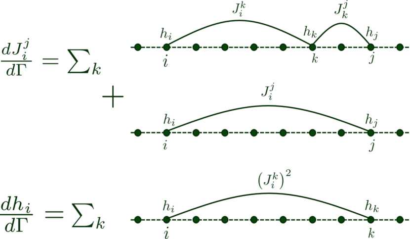
The equation of motion obtained in Eq. (5) leads to the following flow equations for the couplings,

$$\frac{dJ_{i}^{j}}{d\Gamma} = -J_{i}^{j}\left(x_{j}^{i}\right)^{2}-\sum_{k=1}^{N}J_{i}^{k}J_{k}^{j}\left(x_{k}^{j}-x_{i}^{k}\right),$$ (7)

$$\frac{dh_{i}}{d\Gamma} = -2\sum_{k=1}^{N}\left(J_{k}^{i}\right)^{2}x_{i}^{k},$$ (8)

where we have defined, $x_{j}^{i}=h_{i}-h_{j}$. For convenience, we have absorbed a factor of $4$ in the definition of $\Gamma$. The initial conditions for the couplings are $J_{i}^{j}\left(\Gamma=0\right)=J_{i}^{j}$ and $h_{i}\left(\Gamma=0\right)=h_{i}$. As a consequence of the Hamiltonian becoming diagonal in the limit $\Gamma\rightarrow\infty$, we have $J_{i}^{j}\left(\Gamma\rightarrow\infty\right)=0$. The single-particle energy spectrum of the Hamiltonian is obtained from the set of fields in the end of the flow $\left\{h_{i}\left(\Gamma\rightarrow\infty\right)\right\}$. The many-body energies can be found by filling these levels. The flow equations are represented schematically in Fig. 2.

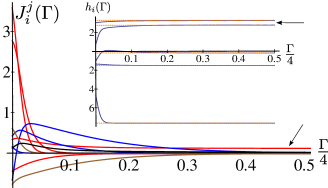
The flow equations can be solved numerically, by starting a chain with random couplings and evolving them numerically via Eqs. (7) and (8). In Fig. 3, we give a comparison of the spectrum obtained using the FE with exact diagonalization for a 5 site chain. The decay of $J_{i}^{j}$ is controlled by the field difference, $h_{i}-h_{j}$. When the final values of $h_{i}$ and $h_{j}$ are close, the decay is much slower, as can be seen also be seen in the Figure.

Figure 3: (Color online) Typical flow for the 5-site problem. The initial fields and hoppings are random variables. The distribution of hoppings is Gaussian, with a power-law decay with distance $\left|i-j\right|^{\alpha}$, $\alpha=1$. The distinct colors represent the different distances $\left|i-j\right|$ (red, blue, brown, and black curves, in order of increasing distance). Notice that one of the red curves, indicated by the arrow, flows more slowly to zero. This is due to the fact that the decay term in the $J$ flow is proportional to difference of the fields of the two sites connected by it [see Eq. (7) and the arrow in the inset curve]. Also shown in the inset is flow of fields (blue) and their asymptotic approach to the Hamiltonian eigenvalues (horizontal dashed orange lines).

In section III.1, we start constructing the phase diagram by exactly solving a chain of two sites. This solution lends a time scale, that allows for a bond-decimation hierarchy. This forms the foundation for an RG scheme described in Section IV, appropriate for $\alpha>1/2$. In section III.2, we develop a scaling approach to follow the distributions of bonds under the evolution of the $N$-site flow equations. The power law exponent of the coupling distribution changes as the couplings flow. From any initial distribution with $\alpha<0.5$, the exponent reaches the universal $\alpha=0$ fixed point. Notice that the combination of the two techniques mentioned above, the direct implementation of the flow equations for $\alpha<1/2$ and the RG scheme developed for $\alpha>1/2$, allows us to map the full phase diagram.

III.1 Building block: Two-site solution

As a first step, let us solve the illustrative example of the two-site chain, with fields $h_{1}$ and $h_{2}$ and inter-site hopping, $J\equiv J_{1}^{2}$. It becomes convenient to define a new variable, $x=h_{2}-h_{1}$. The flow equations, Eqs. (7) and (8), reduce to,

$$\frac{d}{d\Gamma}J\left(\Gamma\right) = -J\left(\Gamma\right)\left(x\left(\Gamma\right)\right)^{2},$$ (9)

$$\frac{d}{d\Gamma}x\left(\Gamma\right) = 4\left(J\left(\Gamma\right)\right)^{2}x\left(\Gamma\right).$$ (10)

These equations have a conserved quantity, which we denote as

$$r^{2}=4J\left(\Gamma\right)^{2}+x\left(\Gamma\right)^{2}.$$

Defining polar coordinates, $J\left(\Gamma\right)=\frac{r}{2}\sin\theta\left(\Gamma\right)$ and $x\left(\Gamma\right)=r\cos\theta\left(\Gamma\right)$, we obtain the flow for $\theta\left(\Gamma\right)$:

$$\frac{d\theta}{d\Gamma}=-\frac{1}{2}r^{2}\sin 2\theta\left(\Gamma\right),$$ (11)

where the initial condition is $\theta_{0}=\theta\left(0\right)=\arctan\left(\frac{2J}{x}\right)$. The solution of this equation is

$$\tan\theta\left(\Gamma\right)=\tan\theta_{0}\exp\left(-r^{2}\Gamma\right).$$ (12)

Asymptotically, as $\Gamma\rightarrow\infty$, $\theta$ tends to zero: $\theta\left(\Gamma\rightarrow\infty\right)=0$. The decay rate of $\tan\theta\left(\Gamma\right)$, gives us a natural RG time scale to achieve a nearly diagonal Hamiltonian:

$$\tau_{\Gamma}\sim\frac{1}{r^{2}}.$$ (13)

In this chain of two sites, the master equation for the distribution of couplings, $J\left(\Gamma\right)$ and $x\left(\Gamma\right)$, can also be exactly solved. The solution reveals that the distributions of $\log J\left(\Gamma\right)$ and $x\left(\Gamma\right)$ are correlated, what can be tracked back to the constraint that $x^{2}\Gamma=-\log\left(J\right)$. Analogous correlations between $J$ and $x$ variables are also observed for the couplings in larger chains. The details are provided in Appendix C.

It is important to note that the two-site flow gives rise to the following canonical transformation of the second-quantized creation operators:

$$\left(\begin{array}[]{c}\tilde{c}_{1}\\ \tilde{c}_{2}\end{array}\right)=\left(\begin{array}[]{cc}\cos\alpha_{12}&\sin\alpha_{12}\\ -\sin\alpha_{12}&\cos\alpha_{12}\end{array}\right)\left(\begin{array}[]{c}c_{1}\\ c_{2}\end{array}\right)$$ (14)

where $\alpha_{12}=\mbox{sgn}\left(Jx\right)\frac{\theta_{0}}{2}$.

III.2 $N$-site problem

Now we consider the full coupled flow equations for the $N$-site problem. Let us start by defining new hopping variables, $G_{i}^{j}=J_{i}^{j}l^{-\alpha}$, where $l=\left|i-j\right|$. We consider the initial distributions for the couplings $J\left(l=\left|j-i\right|\right)$ to have a variance that scales with length as $\sigma_{J}^{2}\left(l\right)\sim l^{-2\alpha}$, while the $G\equiv G_{i}^{j}$ distributions are distance independent. Without loss of generality, assume that $j>i$. The FE in Eq. (7) rewritten in terms of $G$ is

$$-\frac{dG}{d\Gamma} = \sum_{k=1}^{N}X_{k}\left[\frac{l}{\left|k-i\right|\left|j-k\right|}\right]^{\alpha}+G\left(x_{j}^{i}\right)^{2},$$ (15)

$$= \Delta\left(l\right)+G\left(x\left(l\right)\right)^{2}$$ (16)

where $X_{k}=G_{i}^{k}G_{k}^{j}\left(x_{k}^{j}-x_{i}^{k}\right)$. There are two terms in Eq. (15). The term $G\left(x\left(l\right)\right)^{2}$ is responsible for the decay in the magnitude of $G$, and $\Delta\left(l\right)$ acts as a random-source term that generates hoppings distributions with changing power laws, which modifies the distribution of $G$. In order to unveil how this process happens, we ignore the decay term for a moment and consider the scaling of the variance of the distribution of $\Delta\left(l\right)$ at long distances, $\sigma_{\Delta}\left(l\right)$. Let us assume that $X_{k}$ is a scale-independent uncorrelated random variable, $\left\langle X_{k}X_{k^{\prime}}\right\rangle=\left\langle X^{2}\right\rangle\delta_{kk^{\prime}}$. With this assumption, we end up with

$$\sigma_{\Delta}^{2}\left(l\right) = \left\langle X^{2}\right\rangle\left[\sum_{\begin{subarray}{c}k=1\\ k\neq\left\{i,i+l\right\}\end{subarray}}^{N}\frac{l^{2\alpha}}{\left|k-i\right|^{2\alpha}\left|l-\left(k-i\right)\right|^{2\alpha}}\right],$$ (17)

$$= \left\langle X^{2}\right\rangle l^{2\alpha}\left[\int_{1}^{l}\frac{dx}{x^{2\alpha}\left(l-x\right)^{2\alpha}}+\left(\int_{1}^{i-1}+\int_{1}^{N-j}\right)\frac{dx}{x^{2\alpha}\left(l+x\right)^{2\alpha}}\right]$$

The integral is dominated by possible divergences at $x=0$ and $x=l$. Consider first $\alpha<\frac{1}{2}$. It is clear that we can completely scale out $l$,

$$\int_{1}^{l}\frac{dx}{x^{2\alpha}\left(l-x\right)^{2\alpha}}\sim l^{1-4\alpha}\int_{\frac{1}{l}}^{1}\frac{dx}{x^{2\alpha}\left(1-x\right)^{2\alpha}}\propto l^{1-4\alpha},$$

and, therefore, we expect $\sigma_{\Delta}^{2}\left(l\right)\propto l^{1-2\alpha}$. In contrast, at $\alpha=\frac{1}{2}$, the variance is logarithmically dependent on $l$, $\sigma_{\Delta}^{2}\left(l\right)\propto\log l$, hinting a critical behavior. Finally, we note that for the case of $\alpha>\frac{1}{2}$, the variance is independent of the length scale, $\sigma_{\Delta}^{2}\left(l\right)\sim\text{const}$.

Figure 4: (Color Online) The standard deviation of distributions of $J_{i}^{j}$, $\sigma\left(J_{i}^{j}\right)$, as a function of distance $l=|i-j|$ for different RG times $\Gamma$. The simulations were run for system size $N=45$ and averaged over $100$ realizations. The initial distribution of the bonds is Gaussian with standard deviation, $\sigma\left(J_{i}^{j}\right)_{\Gamma=0}=\frac{1}{2|i-j|}$ (red straight lines in log-log scale). The fields $h_{i}$ are chosen to be uniformly distributed between $0$ and $1$. For initial distributions with exponents $\alpha<0.5$, the exponent changes and flows to $\alpha=0$ as $\Gamma$ increases. For exponents, $\alpha>0.5$, the long-distance tails are not altered by the flow.

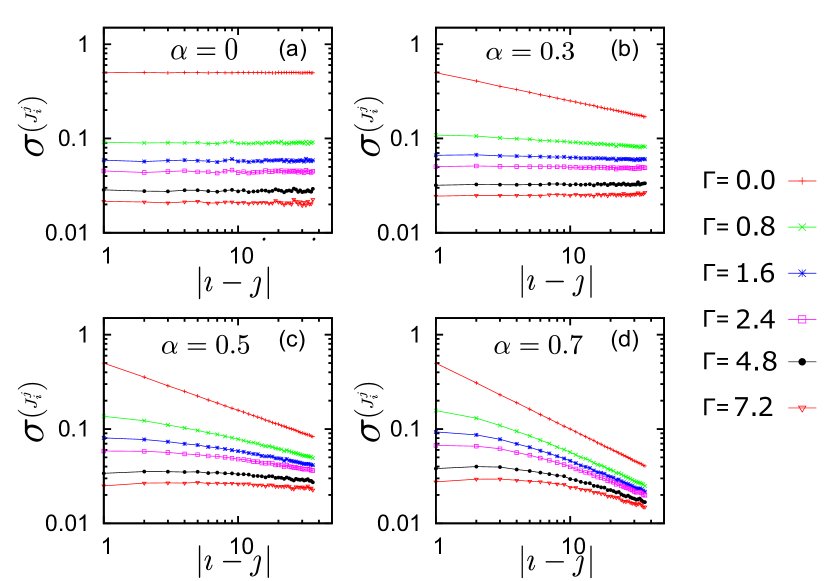
It is apparent from the scaling of the source terms that the $l$-dependence of the variance of the hopping distribution gets modified throughout the flow, since $l^{-2\alpha}\rightarrow l^{1-4\alpha}$ if $\alpha<1/2$. The point $\alpha^{*}=1/2$ is a scaling fixed point, which is also confirmed by the sub-leading logarithmic dependence of the variance of the source terms, $\sigma_{\Delta}^{2}$. Considering parameters slightly away from this fixed point, $\alpha=\alpha^{*}-\epsilon$, the exponent generated by the source term is such that $\alpha^{*}-2\epsilon<\alpha$. Qualitatively, this means that as the RG time scale $\Gamma$ increases, the source term generates distributions with smaller exponents, which become the dominant contribution at long distances. Eventually, the distribution must flow to $\alpha=0$, since $\alpha<0$ is physically not allowed. In the regime $\alpha>1/2$, on the other hand, we see that the source terms have a distribution with a variance that scales as $\bar{\sigma}_{\Delta}^{2}\sim l^{-2\alpha}$. This means that the source terms do not modify the long distance ($l\rightarrow\infty$) behavior of the distribution of $J\left(l\right)$ variables.

In order to check the above argument, we numerically solve Eqs. (7) and (8). The simulations are done for chains with $N=45$ sites, and the $\Gamma$ parameter flows from $\Gamma=0$ until $\Gamma=\Gamma_{\mbox{max}},$ where $\Gamma_{\mbox{max}}$ is chosen according to the disorder strength of the hoppings in such a way that at $\Gamma_{\mbox{max}}$ the energies converge to a fixed value, up to machine precision. We follow the evolution of both $J_{i}^{j}$ and $h_{i}$ as function of $\Gamma$, for chains of $N=45$ sites, and average the results over 100 disorder realizations.

The standard deviation of the distribution $P_{l,\Gamma}\left(J\right)$, $\sigma_{J,\Gamma}\left(l\right)$, as a function of $l$ for several RG times $\Gamma$ is shown for distinct exponents in Fig. 4. Figures (a) and (b) of Fig. 4 illustrate that distributions with exponents $\alpha<\frac{1}{2}$ flow to distributions with a constant standard deviation, that is, $\sigma_{J,\Gamma}\left(l\right)\sim\text{const}$, which corresponds to the behavior of $\alpha=0$. At $\alpha=\frac{1}{2}$, the subleading $\log l$ contribution cannot be seen due to the limitations of the system size. In contrast, for $\alpha=0.7$, the long distance power-law behavior of the standard deviation is unaffected by the RG flow, $\sigma_{J,\Gamma}(l)\sim l^{\-\alpha}$, as shown in Fig. 4(d), in agreement with the previous scaling analysis.

III.3 Operator Flow

Localization of single particle wave functions can be probed by studying the flow of single particle operators. One case of particular interest is the number operator, $c_{i}^{\dagger}c_{i}$, that measures the diffusive character of particles in the chain. We show next that it is possible to study the localized or extended nature of the system studying the evolution of such operators.

Figure 5: Final evolution $\left(\Gamma\rightarrow\infty\right)$ of the number operator initialized in the middle of a $45$-site chain, at site number $23$, $\mathfrak{n}_{23}(\Gamma=0)=c^{\dagger}_{23}c_{23}$, for some representative exponents. At $\Gamma=0$, all $\mathfrak{J}_{23}^{i}$ are zero, and only $\mathfrak{h}_{23}$ is equal to one.The asymptotic values are obtained by measuring the final values of $\left(\mathfrak{J}_{23}^{i}\right)^{2}$ (see Eq. (19)). The tilde indicates the set of variables related to decomposition of the operator flow in terms of an instantaneous basis (Eq. (18)).The results are averaged over 20 disorder realizations.

As the generator $\eta$ evolves with $\Gamma$ according to Eq. (4), any arbitrary operator in the Hilbert space also flows, governed by a Heisenberg equation that is analogous to Eq. (5). Let us now consider the evolution of the number operator at site $k$ as a function of the RG time. Writing the local density operator as, $\mathfrak{n}_{k}\left(\Gamma\right)$, the decomposition in terms of the instantaneous states of $n_{k}\left(\Gamma\right)=c_{k}^{\dagger}\left(\Gamma\right)c_{k}\left(\Gamma\right)$ is

$$\mathfrak{n}_{k}\left(\Gamma\right)=\sum_{i}\mathfrak{h}_{i}\left(\Gamma\right)n_{i}+\sum_{\left\langle i,j\right\rangle}\mathfrak{J}_{i}^{j}\left(\Gamma\right)c_{i}^{\dagger}c_{j},$$ (18)

with the initial condition, $\mathfrak{h}_{i}\left(\Gamma=0\right)=\delta_{ik}$ and $\mathfrak{J}_{i}^{j}\left(\Gamma=0\right)=0$. We find the general flow equations for these operator variables to be

$$\frac{d\mathfrak{J}_{i}^{j}}{d\Gamma} = -J_{i}^{j}x_{j}^{i}\mathfrak{x}_{j}^{i}-\sum_{k=1}^{N}\mathfrak{J}_{i}^{k}J_{k}^{j}x_{k}^{j}+\sum_{k=1}^{N}J_{i}^{k}\mathfrak{J}_{k}^{j}\left(x_{i}^{k}\right),$$ (19)

$$\frac{d\mathfrak{h}_{i}}{d\Gamma} = -2\sum_{k=1}^{N}J_{k}^{i}\mathfrak{J}_{k}^{i}x_{i}^{k},$$ (20)

where $\mathfrak{x}_{i}^{j}=\mathfrak{h}_{j}-\mathfrak{h}_{i}$. As $\Gamma\rightarrow\infty$, we obtain $\tilde{n}_{k}$ expressed in the basis of the eigenfunctions of the Hamiltonian. Since the evolution of the operator variables is intrinsically constraint to the couplings of the Hamiltonian, their flow correlates with the flow of the set $\left\{h_{i},J_{i}^{j}\right\}$.

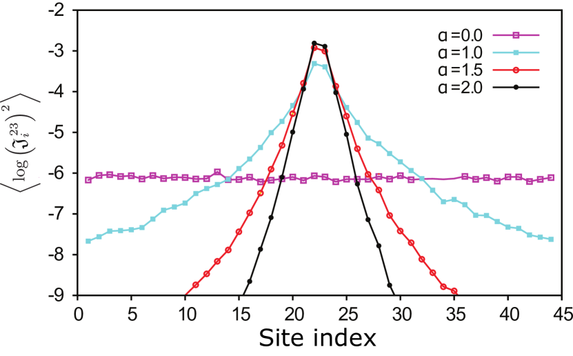
The flow equations, Eqs. (19) and (20) can be solved numerically. We choose the initial point $k$ to be the midpoint of the chain ($N=22$), and plot the value of $\left(\mathfrak{J}_{i}^{k}\right)^{2}$ as a function of the distance $\left|i-k\right|$, averaged over 20 disorder realizations. The results are shown in Fig. 5 for different exponents $\alpha$. For large exponents, $\alpha>1$, the decay is exponential (linear in log scale), indicating that the density operator stays localized or, equivalently, that the initial particle fails to diffuse as a consequence of the localization of the wavefunctions. For small exponents, $\alpha<1$, the operator reaches a significant value even at sites arbitrarily far from the middle, indicating the possibility of long-ranged resonances. The precise transition point cannot be found due to the restriction of the system size, but the existence of two phases can already be inferred. The precise critical point is going to be discussed later, via other numerical and analytic methods.

One of the handicaps of the flow equation technique, is that it requires the solution of $\mathcal{O}\left(N^{2}\right)$ coupled differential equations. This is generally time consuming; the advantage over exact diagonalization, however, lies with the ability to extract universal features of the system directly from the flow. In the next section, we simplify the flow equations further, into a set of decoupled equations, solved sequentially. This strong-bond RG method, allows us to solve the full set of equations efficiently (although still at an $\mathcal{O}(N^{3})$ cost). It works in the regime, $\alpha>\frac{1}{2}$, where we show that our assumptions are correct and the errors accumulated are vanishing in the thermodynamic limit. We use this method to gain further insights into the delocalization transition.

IV Strong-bond RG method

The exact two-site solution allows us to devise an RG-scheme of sequential transformations. These transformations produce an alternative scheme for constructing the unitary that diagonalizes the Hamiltonian, and it can also efficiently yield an approximate solution of the flow in Eqs. (7) and (8). As we noted in Section III.1, the FE diagonalizes the two-site problem with a characteristic RG timescale, $\tau_{\Gamma}\sim\frac{1}{r^{2}}$. This suggests an approximate solution to the $N$-site problem by breaking it into a sequence of two-site rotations ordered by the magnitude of $r$. Each rotation sets the hopping across the bond to zero. At every RG step, we transform the bond given with the largest value of $r$ and renormalize the bonds connected to sites of the decimated bond. In Fig. 6, we schematically show the RG procedure.

This RG procedure can be interpreted as an ordered sequence of two-site rotations, analogous to the Jacobi algorithm used to diagonalize matrices [42]. The difference from the Jacobi rotation method is that the FE provides a natural ordering the decimations, the descending value of $r$.

Figure 6: (Color Online) Schematic of the steps in the Strong-bond RG method. The first part consists of finding the bond $\left(i,j\right)$ with the maximum $r_{ij}$. Using an appropriate unitary, the hopping on the bond is transformed to zero. Hoppings connecting to the bond, $\left(\tilde{J}_{i}^{k},\tilde{J}_{j}^{k}\right)$, and fields on its sites $\left(\tilde{h}_{i},\tilde{h}_{j}\right)$, are renormalized. This procedure is iterated until all bonds are set to zero. The strong disorder allows is to make a crucial simplification: Once a bond is set to zero, we neglect its regeneration in subsequent steps. This produces a negligible error if the generated $\tilde{r}_{ik}$ and $\tilde{r}_{jk}$ are smaller than the removed $r_{ij}$. After $\mathcal{O}\left(N^{2}\right)$ steps, where $N$ is the system size, the Hamiltonian is diagonal.

The strong-bond RG procedure relies on the two-site transformation, Section III.1. In practice, we employ the 2-site transformation as a Jacobi rotation on the entire Hamiltonian. The guidance provided from the flow-equations is the order in which we should pursue the transformations. Relegating the details of the rotations to App. F, we provide here the resulting RG procedure steps:

1. Find the largest non-decimated $r$, say $r_{\textrm{max}}=r_{ij}=\sqrt{4\left(J_{i}^{j}\right)^{2}+x_{ij}^{2}}$, between sites $\left(i,j\right)$.

2. Compute the corresponding bond angle

   $$\alpha_{ij}=\mbox{sgn}\left(J_{i}^{j}x_{i}^{j}\right)\frac{\theta_{i}^{j}}{2},$$ (21)

   where

   $$x_{i}^{j}=h_{j}-h_{i},$$ (22)

   and

   $$\theta_{i}^{j}=\arctan\left|\frac{2J_{i}^{j}}{x_{i}^{j}}\right|.$$ (23)

3. Set the corresponding $J_{i}^{j}$ to zero.

4. Renormalize all bonds connected to sites $i$ or $j$ according to:

   $$\tilde{J}_{i}^{k} = J_{i}^{k}\cos\left(\alpha_{ij}\right)+J_{k}^{j}\sin\left(\alpha_{ij}\right),$$ (24)

   $$\tilde{J}_{j}^{k} = -J_{i}^{k}\sin\left(\alpha_{ij}\right)+J_{j}^{k}\cos\left(\alpha_{ij},\right).$$ (25)

   where $\alpha_{ij}$ was defined in Eq. (21).

5. Renormalize the fields $h_{i}$ and $h_{j}$ according to

   $$\tilde{h}_{i,j} = \frac{1}{2}\left[H_{ij}\pm r_{\textrm{max}}\mbox{sgn}\left(x_{i}^{j}\right)\right],$$ (26)

   where $H_{ij}=h_{i}+h_{j}$.

6. Compute the renormalized values of $r$: $\tilde{r}_{ik}$ and $\tilde{r}_{jk}$.

The number of steps until the Hamiltonian becomes diagonal scales as $\mathcal{O}(N^{2})$, where $N$ is the system size. Each step renormalizes $\mathcal{O}(N)$ bonds connected to the decimated bond. Therefore, the number of computations necessary to compute all eigenvalues using this method is $\mathcal{O}(N^{3})$. Also, in this RG proposal, each diagonal element, that converges to the approximate eigenvalue, is renormalized $\mathcal{O}\left(N\right)$ times. This is an advantage in comparison to other proposals, like the one by Javan Mard et al.[37], for example, if one is interested in level spacing. In the latter RG proposal, sites, and not bonds, are removed from the chain. This procedure also coincides with the procedure in Ref. 16, which was developed simultaneously, and applied to many-body systems.

IV.1 Universal properties from the strong-bond RG

The strong bond renormalization group approach primarily provides a new perspective from which the universal properties of disordered quantum systems could be extracted. First, the successive RG transformations suggest representing the problem as a 2-dimensional scatter plot on the $x-J$ plane. Each point in the plot corresponds to a particular bond connecting two sites, say $i$ and $j$. Its “y” value is the bond strength $J_{i}^{j}$, and its “x” value is the difference of the on-site fields $\left\{h_{i},h_{j}\right\}$, $x_{i}^{j}=h_{j}-h_{i}$. A diagonal Hamiltonian, for example, would correspond to having all points on the $x_{i}^{j}$ axis.

The emerging picture provides a convenient way to represent the RG flow of the coupling distribution under the scheme of the previous Section, IV. As shown schematically in Fig. 7, a decimation corresponds to rotating bonds in the largest circular shell, bringing them to the $x_{i}^{j}$ axis. In the later steps, the points within the circle get modified according to the Eqs. (24), (25), and (26). Let us call it $P_{\Gamma}\left(x\right)$ the distribution of $x_{i}^{j}$ at scale $\Gamma$. As one decimates all the bonds in the Hamiltonian, the final distribution of points on the $x_{i}^{j}$ axis is obtained. The final distribution, $P_{\Gamma\rightarrow\infty}\left(x\right)$, is the distribution of the level separations for all the eigenvalues of the Hamiltonian. It is proportional to the level correlation function [39] which, in the limit $x\rightarrow 0$, is identical with the level spacing statistics. For simple localized and extended states it is given by

$$\lim_{x\rightarrow\infty}P_{\Gamma\rightarrow\infty}\left(x\right)\propto\begin{cases}\text{ const.},&\text{if the phase is localized}\\ x,&\text{if the phase is extended}.\end{cases}$$ (27)

Examining the long RG-time fixed points of the flow of the distributions, therefore, allows us to identify the different phases of a system, and extract their universal properties.

Figure 7: (Color Online) The representation strong bond RG procedure in the $x-J$ space. Each point represents a bond, and its distance from the origin is $r_{ij}$. the strong bond RG rotates the bonds within a large-$r$ shell. In the first step, the bonds with largest $r_{i}^{j}$ are rotated to the $x_{i}^{j}$ axis. Next, the bonds connected to the decimated bond undergo a renormalization via Eqs. (24), (25), and (26). We perform one approximation: once eliminated, a bond is not allowed to assume finite values again, and these points which lie on the $x$-axis beyond the $r$-cutoff move horizontally only.

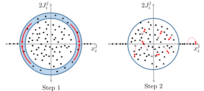
The $x-J$ space gives an intuitive picture for how the level-spacing distributions emerge in the two fixed points of the PBRM model - the localized and extended phases. A level repulsion, as in the extended phase, is obtained from a uniform distribution of bonds in the $x-J$ space of Fig. 7. In contrast, for localized states that do not repel each other, the joint distribution has a finite range in the phase space with a length scale $\xi\ll r_{\textrm{max}}$. As a simplification, we assume that the effect of the bond renormalization, which is schematically represented in Fig. 7, can be ignored. First consider the case of a uniformly distributed bonds in the phase space, $P_{\Gamma}\left(J,x\right)\sim\text{const.}$ In this case, the number of decimations in a circular shell of radius $r_{\text{max}}$ and width $dr_{\mbox{max}}$ is $N_{\text{dec}}\propto 2\pi r_{\text{max}}dr_{\text{max}}$. The number of decimations fixes the distribution of bonds at $x=r_{\text{max}}$. Therefore, we have the distribution

$$P_{\Gamma}\left(x\right)dx\sim r_{\text{max}}dr_{\text{max}}\sim xdx,$$ (28)

which correctly reproduces the Wigner-Dyson statistics in the limit of small level spacing. Now, we can repeat the same analysis for $P_{\Gamma}\left(J,x\right)\sim e^{-J/\xi}$. In this case, the number of decimations goes as $N_{\text{dec}}\propto\xi dr_{\text{max}}$. Consequently, we have for the distribution of level separations

$$P_{\Gamma}\left(x=r_{\text{max}}\right)\sim\text{const},$$ (29)

consistent with Poisson statistics for localized states at the small level spacing limit. We note that this analysis relies on the assumption that the renormalization of the bonds does not significantly alter the marginal distribution of $J$. In the following, we show that this approximation is reasonable. Note that the bond distribution function in the $x-J$ space typically separates into a product distribution, with a uniform distribution on the x-axis at late stages of the flow. The J-distribution then arbitrates the level statistics: If it is uniform, we obtain Wigner-Dyson statistics, and if it is concentrated near $J=0$, a Poisson-type distribution emerges.

IV.2 Strong-bond RG and the delocalization transition

Let us consider the effects of bond renormalization on the marginal bond distribution, $P_{\Gamma}\left(J\right)$ of the PBRM model. Examining Eqs. (24) and (25), the evolution of the bonds $J$ may be interpreted as a random walk with an amplitude proportional to $J$. To be more precise, the variance of the bonds change under renormalization as

$$\sigma^{2}\left(\tilde{J}_{i}^{k}\right)\approx\left\langle\left(J_{i}^{k}\right)^{2}\right\rangle+\left\langle\left(J_{j}^{k}\right)^{2}-\left(J_{i}^{k}\right)^{2}\right\rangle\sin^{2}\alpha_{ij}$$ (30)

where we have assumed that the product $J_{i}^{k}J_{j}^{k}$ is uncorrelated, $\left\langle J_{i}^{k}J_{j}^{k}\right\rangle\sim\left\langle J_{i}^{k}\right\rangle\left\langle J_{j}^{k}\right\rangle=0$. The rotation angle $\alpha_{ij}$ is defined in Eq. (21). The change of the standard deviation is reminiscent of a one-dimensional random walk with a variable amplitude for each of the steps. Furthermore, we can assume that the two bonds that are renormalized, $J_{i}^{k},\,J_{j}^{k}$ are of comparable range. The change in variance is then:

$$\left|\Delta\left\langle\left(J_{i}^{k}\right)^{2}\right\rangle\right|\sim\left\langle\left|\left(J_{i}^{k}\right)^{2}-\left(J_{j}^{k}\right)^{2}\right|\right\rangle\sim\left\langle\left(J_{i}^{k}\right)^{2}\right\rangle,$$ (31)

where, note that the average change is non-zero because we are computing the magnitude. So the random change in the magnitude of the bond is proportional to the bond strength itself. Relying on this insight, we can model the flow of the $J$ distribution as a diffusion equation with a $J$-dependent diffusion constant, $D\left(J\right)=D_{0}J^{2}$. Before writing the equation, we note that the sum of undecimated couplings, $\sum\limits_{i\neq j}\left(J_{i}^{j}\right)^{2}$, remains constant throughout the RG flow. We account for that by adding a rescaling term in the diffusion equation. The combined equation is then:

$$\frac{\partial P_{\Gamma}\left(J\right)}{\partial\Gamma}=\frac{\partial}{\partial J}\left(D_{0}J^{2}\frac{\partial P_{\Gamma}\left(J\right)}{\partial J}-\gamma JP_{\Gamma}\left(J\right)\right),$$ (32)

where the values of the diffusion constant $D_{0}$ depend on the details of the distributions of $J$ and $x$ at the renormalized scale. $\gamma$ is a Lagrange multiplier which is adjusted to maintain the variance of the problem constant.

The steady states of Eq. (32) are easy to infer. From the structure of the diffusion equation we see that the solutions must be scale invariant, i.e., power-law distributions. For any power low distribution,

$$P_{\Gamma}\left(J\right)\sim C\left(\Gamma\right)J^{-\beta},$$ (33)

the exponent $\beta$ would remain invariant. Furthermore, since $\gamma$ is adjusted to maintain the variance of $J$ constant, the $\gamma$ rescaling term would actually make any power-law distribution a fixed point.

The discussion above makes us consider what appears to be the most crucial feature of the PRBM. The initial hopping distribution $P_{\Gamma=0}(J)$ for the power-law decaying random hopping is already a power law for almost all $J$’s. Therefore, it is a fixed-point distribution from the start. In more detail, the initial marginal bond distribution of all bonds $P_{\Gamma=0}\left(J\right)$ for a length $N$ chain has two distinct behaviors. At small $J$’s, with $J<J_{c}=\frac{1}{N^{\alpha}}$ it is uniform, and for $J>J_{c}$, it is a power law:

$$P_{\Gamma=0}\left(J\right)\propto\begin{cases}\frac{1}{J^{1+1/\alpha}}&,\text{for }J>J_{c}\\ N^{\alpha}&,\text{for }J<J_{c}\end{cases}$$ (34)

This is calculated and numerically verified in Appendix D. Since each of the two segments is a power-law, both remain invariant. The crossover range, however, may change in the flow. Any changes of $J_{c}$ during the flow, however, are bound to result in a scale-invariant change. Therefore, we assume that $J_{c}\sim 1/N^{\alpha}$ throughout the flow. This expectation is confirmed by our numerics, as discussed in the next section.

Figure 8: (Color Online) Marginal distribution $P_{\Gamma}\left(\log J\right)$ in the log scale for different RG steps $\Gamma$. From (a) to (c), we plot the evolution of the marginal distribution for exponents $\alpha=0.7$, $\alpha=1.0$ and $\alpha=2.0$. Different colors represents different RG steps; $\Gamma=1$, $1000$, $2000$, $3000$ are represented by blue, red, green, magenta, and black, respectively. As seen from Eq. (34) there are two distinct regimes in the probability distribution. The crossover scale is given by $J_{c}$. Below this, $J<J_{c}$, $P_{\Gamma}\left(\log J\right)\sim\log J$ and above the scale, for $J>J_{c}$, $P_{\Gamma}\left(\log J\right)\sim-\frac{1}{\alpha}\log J$. We note that as the bonds are decimated, the behavior of the distribution below and above the crossover remains unchanged. The system has size $N=100$ and we average over 20 disorder realizations.

Now we can address the critical behavior of the power-law hopping problem. The fact that any power-law marginal $J$ distribution is also marginal in the RG sense implies that the entire $\alpha>0.5$ parameter range is critical. The transition, we show, emanates from the size dependence of the marginal distribution. The two regimes of $P_{\Gamma}(J)$ also imply two regimes of level spacings. After very little flow, the marginal $x$ distribution flattens, and the full x-J bond density is:

$$P(x,J)\approx c\frac{r_{\textrm{max}}}{r_{0}}N^{2}P_{\Gamma}(J)$$ (35)

where $c$ is a constant, and $r_{\textrm{max}}$ is the RG cutoff, and $r_{0}$ is the largest RG cutoff. As we transform away bond in the arc $r_{\textrm{max}}-dr<r<r_{\textrm{max}}$, and reduce $r_{\textrm{max}}$, the number of bonds affected, and hence the density of level spacings is:

$$\rho(x)\sim\left\{\begin{array}[]{cc}\textrm{const},&r>J_{c}\\ c\,\,r&r<J_{c}\end{array}\right.$$ (36)

Next, we need to find out how the mean level spacing, $\bar{\delta}$, scales. For $\alpha>1/2$, we expect $\bar{\delta}_{N}\sim\frac{1}{N}$, since the system’s bandwidth is size independent. In Appendix E we demonstrate this result under the flow-equations scope. Alternatively, we can use the fact that the bandwidth of the Hamiltonian, $W$, is bounded by the norm of the off-diagonal terms, added to the disorder width $w_{0}$ :

$$W\leq w_{0}+\sqrt{\int_{0}^{N}dl\ J_{\textrm{typ}}^{2}\left(l\right)}\propto N^{\frac{1}{2}-\alpha}+\text{const.},$$ (37)

where $J_{\textrm{typ}}\left(l\right)\propto\frac{1}{l^{\alpha}}$, are the length-dependent hopping terms. In the thermodynamic limit, when $\alpha>1/2$, the length-dependent correction vanishes.

The phase of the system, and the delocalization transition, are inferred from the level-spacing statistics, expressed in terms of the rescaled level spacing. We denote the rescaled level spacing as $\bar{\epsilon}=\epsilon/\bar{\delta}_{N}$. As Eq. (36) shows, level repulsion appears below the energy difference $J_{c}$. In terms of the scaled level spacing, this implies that level-repulsion sets in for rescaled energy difference:

$$\bar{\epsilon}_{c}(N)\approx\frac{{J_{c}}}{{\bar{\delta}_{N}}}\sim N^{1-\alpha}.$$ (38)

For $\alpha>1$, $\bar{\epsilon}_{c}$ vanishes in the thermodynamic limit. When $\alpha\leq 1$, the crossover point $J_{c}$ is non-negligible in the thermodynamic limit. When the decimation scale reaches $J_{c}\sim 1/N^{\alpha}$, the distribution of bonds becomes uniform in the $J-x$ phase space. For $\alpha<1$, the level repulsion emerges at $\epsilon_{c}\sim N^{1-\alpha}\bar{\delta}_{N}$, which is much larger than the average level spacing. On the other hand, for $\alpha>1$, $\epsilon_{c}\ll\bar{\delta}_{N}$ and, therefore, the distribution of level spacings is Poissonian. The phase diagram of Fig. 1 emerges naturally from the strong-bond RG analysis.

The strong-bond RG picture also yields the correlation length scaling of the transition. Let us define $\xi$ as the chain length that allows us to determine the phase of the system from the level-statistics distribution. In the delocalized phase, $\alpha<1$, we would require $\epsilon_{c}(\xi)>a\bar{\delta}_{\xi}$, with $a>1$ being some constant, which we could set to be $a=2$ without loss of generality. This would imply $\xi^{1-\alpha}=a$, and:

$$\xi_{del}\sim a^{1/(1-\alpha)}.$$ (39)

Similarly, in the localized phase, $\alpha>1$, level repulsion will always emerge at some finite energy scale, as the scaling of $\epsilon_{c}(N)$ suggests. This scale, however, must be well below the average level spacing. We would then require $\epsilon_{c}(\xi)<\bar{\delta}_{\xi}/a$. This leads to:

$$\xi_{loc}\sim a^{1/(\alpha-1)}.$$ (40)

Together, Eqs. (39) and (40) imply:

$$\ln\xi\sim\frac{1}{|\alpha-1|}$$ (41)

which is consistent with the results of Ref. 7. In this analysis, we note that the localization length for $\alpha>1$, becomes the correlation length in the delocalized regime, for $\alpha<1$.

IV.3 Numerical results

Figure 9: Decimated $r=r_{\mbox{max}}$ as function of the RG step in a given disorder realization, for distinct exponents, (a) $\alpha=0.1$, (b) $\alpha=0.7$, (c) $\alpha=1.0$, and (d) $\alpha=2.0$. The behavior of the slopes of the peaks in the curves differs significantly, as in (a) $r$ increases in several consecutive RG steps, while in (b-d) a bond that is generated with $r>r_{\text{max}}$ is immediately removed. Notice additionally that, in contrast with (a), in (b-d) the decimated $r_{\text{max}}$ decreases consistently during the RG flow.

The scaling statements made above in Sec. IV.2 were confirmed numerically. In Fig. 8, we plot the marginal distribution $P\left(J\right)$ for different RG steps. Clearly, when $r_{\text{max}}>J_{\text{cross}}$, the exponent of the initial power law remains unchanged. In contrast, below the cutoff the bonds are uniformly distributed.

The method is reliable for $\alpha>0.5$, it is asymptotically accurate as $\alpha\rightarrow\infty$ when all states are localized, and it fails in the strongly delocalized regime, $\alpha<0.5$. The failure in the $\alpha<0.5$ region can be traced to the approximation that a transformed bond is not regenerated: once removed, the corrections to a transformed bond are neglected in later RG steps. This assumption is crucial for the formulation of an RG flow, since such flow relies on a decreasing scale, $r$. This approximation, however, breaks down when one of the renormalized bonds, $\tilde{r}_{ik}$ or $\tilde{r}_{jk}$, is greater than $r_{ij}$. Such “bad decimations” correspond to cases when delocalized clusters of three or more sites should be diagonalized simultaneously.

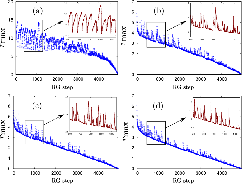
The numerical implementation of our RG method can also be used to obtain the eigenvalues of particular realizations of the problem. Fig. 9 contrasts the evolution of $r_{\textrm{max}}$ during the RG flow for the different phases. For $\alpha<\frac{1}{2}$, the $r$ values of transformed bonds increase as a function of the decimation step (Fig. 9a). Indeed, in this regime the two-site solution is not applicable; the full flow equations of Section III, that can describe macroscopically large clusters, are needed. This effect, however, is absent for $\alpha>0.5$, including at the transition point, $\alpha=1$. In those cases, RG steps occasionally generate a family of large $r$’s. But these $r$’s are promptly eliminated, and $r_{\textrm{max}}$ continues to monotonically decrease, and the method is controlled.

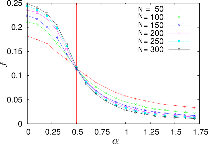
We also considered the number of bad decimations as a function of system size. Remarkably, the fraction of bad decimations vanishes in the thermodynamic limit for all $\alpha>0.5$, as shown in Fig. 10. Our plot shows a crossing at $\alpha=\frac{1}{2}$, which is the transition point from intermediate level statistics to GOE level statistics. This figure reveals that the method fails only for the strongly delocalized part of the phase diagram. The RG procedure is valid at and around the localization-delocalization critical point, $\alpha=1$ and therefore provides an accurate description of the critically delocalized wavefunctions.

Figure 10: Fraction of decimations $\left(\,f\,\right)$ that does not lower the energy scale $r$, in the Strong-bond RG scheme. There is a transition at $\alpha=0.5$, indicating the failure of the Strong-bond RG for $\alpha<0.5$. The Strong-bond RG has vanishing fraction of decimations in the thermodynamic limit for $\alpha>0.5$.

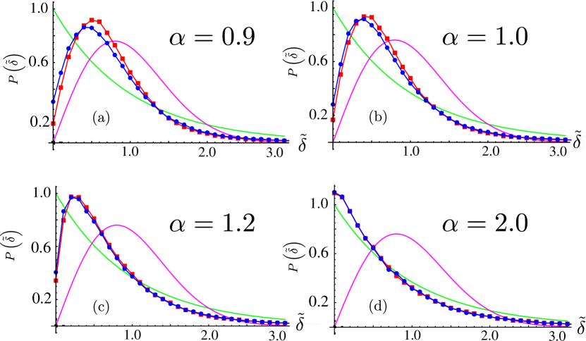
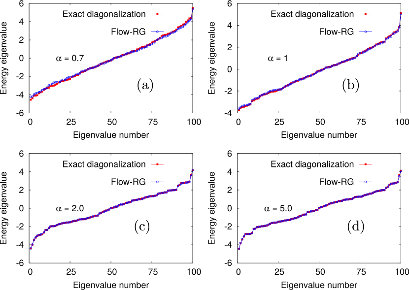
In Appendix F we compare the single particle spectrum and its level statistics obtained from exact diagonalization and the RG procedure in the regime of applicability, $\alpha>0.5$. We see a decent agreement between the strong-bond RG results and exact diagonalization for a variety of $\alpha$ values. We considered chains of 400 sites, and averaged over 500 disorder realizations. We choose $G_{i}^{j}$ and $h_{i}$ to have Gaussian distributions, with unit standard derivation. The level spacings, $\delta$, are computed in units of their mean value. It is well known [43, 40, 39, 44] that random matrices in the GOE ensemble have a universal distribution for the level spacing, $P\left(\delta\right)=\frac{\pi\delta}{2}\exp\left(-\frac{\pi}{4}\delta^{2}\right)$. In contrast, localized Hamiltonians exhibit no level repulsion and hence the level-spacing statistics are Poissonian, $P\left(\delta\right)=\exp\left(-\delta\right)$. As discussed in Section II, the critical point at $\alpha=1$ exhibits intermediate level-statistics that are neither Poisson nor Wigner-Dyson. This feature of the critical level-spacing statistics can be reproduced using the strong-bond RG, as shown in Fig. 11(b) for the critical point. In contrast, for $\alpha=5$, the system is localized at all eigenvalues, and hence the level-spacing statistics are Poisson as shown in Fig. 11(d). Slightly away from the critical point at $\alpha=0.9$, Fig. 11(a), we see that there is a deviation for small $\delta$ in the level repulsion obtained using exact diagonalization and the Strong-bond RG procedure. We attribute this deviation to finite-size effects, which were anticipated in Sec. IV.2. We find, therefore, strong support for all aspects of the strong-bond RG analysis from the numerical results.

Figure 11: (Color Online) Level spacing comparison for eigenvalues obtained through Strong-bond RG (blue circles) and exact diagonalization (red squares), normalized by the mean level spacing value. (a), (b), (c), (d) correspond to exponents $\alpha=0.9$, $1$, $1.2$, and $2$, respectively. For comparison, we also plot the analytical expressions for Poisson (green) and Wigner-Dyson (magenta) statistics. The system size is $N=400$ sites, averaged over $500$ disorder realizations. The $G_{i}^{j}=J_{i}^{j}\left|i-j\right|^{\alpha}$ and $h_{i}$ variables follow Gaussian distributions, with unit standard derivation.

We also observe some universal behavior of the distributions under the RG procedure. Since $\alpha$ remains fixed during the RG flow, we can study the behavior of the distributions of $G=J_{i}^{j}\left|i-j\right|^{\alpha}$. In Fig. 12, we plot the distribution of these bonds $P\left(G_{i}^{j}\right)$ as a function of the decimation step. We illustrate with the case when the initial distributions of the bonds $G_{i}^{j}$ are uniform (from 0 to 1), but we have verified that the behavior is similar if $G_{i}^{j}$ has a Gaussian distribution. Under the RG procedure, after a large number of steps, the bonds become normally distributed. This is a feature not only at the critical point but also away from it. We note that Levitov[36] predicted that the fixed point distribution of bonds is a normal distribution using a real-space RG scheme. We see that the same holds true for the strong-bond RG procedure.

This method also provides us the eigenfunctions of the Hamiltonian. Since each decimation corresponds to a rotation of the basis, the full unitary matrix for diagonalizing the Hamiltonian can be obtained from the product of all the two-site decimations. The eigenfunctions obtained using this method have remarkably close behavior to the exact eigenstates. In the Appendix H, we outline the procedure to obtain the full eigenfunctions of the system. We also calculate the critical, fractal dimensions from the inverse participation ratio (IPR) statistics. This indicates that the method is quite controlled and gives us the correct behavior at the critical point.

Figure 12: (Color Online) Distribution of non-decimated distance-independent bond couplings $G=J_{i}^{j}\left|i-j\right|^{\alpha}$, $\tilde{P}\left(G\right)$, as the RG flows, at RG steps $N_{\textmd{steps}}=1$ (blue), 100 (red), 1000 (green), 2000 (magenta), and 3000 (black). The number of sites is $N=100$, and the total number of steps to diagonalize the Hamiltonian is $N_{\textmd{steps}}=4950$. The exponents shown are (a)$\alpha=0.7$, (b) $\alpha=1.0$, (c) $\alpha=2$. In all cases, the initial distribution of $G$ is uniform, from $-1$ to $1$ (blue curve). At later RG steps, the $G$ distribution becomes Gaussian.

V Conclusions

In this paper, we have shown that the Wegner’s flow equation is a very useful tool to study localization transitions . We choose, for concreteness, the example of non-interacting particles with power-law decaying hoppings. This method allows us to map out the phase diagram of the model as a function of the decay exponent, $\alpha$. The flow equations reveal an attractive fixed point for the distribution of the hoppings at $\alpha=0$, which corresponds to the GOE phase. Rather surprisingly, we find that $\alpha=\frac{1}{2}$ is an unstable fixed point and for $\alpha>\frac{1}{2}$, the distribution of hoppings remains fixed under the flow. The strong-bond RG procedure inspired from the flow equations provides an intuitive description of the emergence of this transition in the level-spacing statistics. The signature we use to probe the localization transition at $\alpha=1$ is in the distribution of the level spacings.

The results discussed in this paper can be generalized to study other systems. The particular advantage of this method is that it preserves the full spectrum of the Hamiltonian. This has implications in studying localization-delocalization transitions in interacting and disordered systems. Many-body localized systems are pseudo-integrable, in the sense that they have a large number of conserved charges with local support [45, 12]. There has been some recent work on studying these conserved quantities using various methods (for instance, see Ref. 16). These conserved quantities can be obtained directly using flow equations, and therefore this method provides a tool to study fully-localized interacting phases, as recently reported in Ref. 46.

In this paper, we have also shown that the strong-bond RG procedure is suitable to study critically delocalized phases. We expect that a similar generalized method should be useful to study the system across the MBL-ergodic phase transition.

Yet another direction to consider is the analytical description of the phases of disordered and interacting systems with power-law decays. In these systems, the strong-disorder renormalization techniques developed so far fails, and the only known results are obtained numerically via exact diagonalization [47]. A strong-disorder renormalization group suitable to handle such systems is still missing. We expect the flow equation technique to be more useful in that task, to study the both zero- and high-temperature phases.

VI Acknowledgments

The authors would like to acknowledge useful discussions with Stefan Kehrein, Sarang Gopalakrishnan, Eduardo Miranda and David Huse. P.T. and G. R. are grateful for support from NSF through DMR-1410435, as well as the Institute of Quantum Information and matter, an NSF Frontier center funded by the Gordon and Betty Moore Foundation, and the Packard Foundation. V.L.Q. acknowledges financial support from FAPESP, through grants 2012/17082-7 and 2009/17531-3.

Appendix A Critical point analysis

In this appendix, we outline the analysis of the the transition as a function of the power law exponent $\alpha$. The results here are an extension of Levitov‘s results for the $\alpha=1$ critical point [36, 6].

Consider an arbitrary site at $r_{i}$ and two concentric one-dimensional “spheres” with radius $2^{k}R<\left|r-r_{i}\right|<2^{k+1}R$, for a given value of $k$. The volume of this shell is $V\left(k,R\right)=2^{k}R$. The characteristic level spacing in this shell, $\Delta\left(k,R\right)$, and the typical hopping strength, $J\left(k,R\right)$, are

$$\Delta\left(k,R\right) \sim \frac{1}{nV\left(k,R\right)},$$ (42)

$$J\left(k,R\right) \sim \frac{1}{\left(2^{k}R\right)^{\alpha}},$$ (43)

where we have assumed a constant density of states $n$. The typical value of the probability distribution for a resonance with site $i$ in this shell is

$$P\left(k,R\right)\propto\frac{J\left(k,R\right)}{\Delta\left(k,R\right)}=\frac{2^{k}R}{\left(2^{k}R\right)^{\alpha}}=\left(2^{k}R\right)^{\epsilon},$$ (44)

where we defined $\epsilon=1-\alpha$. Notice that the volume of the system is $V_{tot}=2^{L}R$. There are three possible cases that must be considered separately. In all cases, we consider additionally the probability of not finding a resonance beyond a $R$, $P_{nr}$. Delocalized phases, as well as the critical point, will have a vanishing $P_{nr}$ for large $R$.

• Critical regime, $\epsilon=0$: $P\left(k,R\right)=b$ is a constant. The probability of not finding a resonance beyond a $R$ is $P_{nr}=\prod_{k=1}^{N}\left[1-P\left(k,R\right)\right]=\left(1-b\right){}^{L}\rightarrow 0$ at the thermodynamic limit. Also, the total number of sites in resonance with site $i$ is

$$N_{res} = \sum_{k=0}^{N}P\left(k,R\right)=\left(L+1\right)b$$ (45)

$$\sim \log\left(V_{tot}\right).$$

• Delocalized regime, $\epsilon>0$: In this case, we take the log to find

$$\log\left(P_{nr}\right) = \sum_{k=0}^{N}\log\left(1-\left(2^{k}R\right)^{\epsilon}\right)$$ (46)

$$= -\sum_{k=0}^{N}\frac{1}{k}\left(2^{k}R\right)^{\epsilon}\sim-R^{\epsilon}2^{\epsilon L}$$

$$\Rightarrow P_{nr} \sim\exp\left(-R^{\epsilon}2^{\epsilon L}\right)\rightarrow 0$$ (47)

Note that, in general, the probability of a resonance $P\left(k,R\right)=1-P_{rn}$ grows with $R$ for $\epsilon>0$ indicating a delocalized regime. In fact, the number of sites at resonance is,

$$N_{res} = \sum_{k=0}^{N}\left(2^{k}R\right)^{\epsilon}=R^{\epsilon}\sum_{k=0}^{N}\left(2^{\epsilon}\right)^{k}$$ (48)

$$= R^{\epsilon}\frac{\left(1-2^{\epsilon\left(N+1\right)}\right)}{1-2^{\epsilon}}\sim R^{\epsilon}2^{\epsilon N}\text{ for }N\gg\frac{1}{\epsilon}$$

$$\propto \left(V_{tot}\right)^{\epsilon},$$

which diverges at the thermodynamic limit. It should also be noticed that such divergence is not extensive in volume, but instead increases with power $\epsilon$.

• Localized Regime, $\epsilon<0$: Similar to the delocalized regime, we set $\epsilon=0^{-}$, then $P_{nr}=\prod_{k=0}^{N}\left(1-\left(2^{k}R\right)^{\epsilon}\right)\sim\exp\left(R^{\epsilon}\right)$. So for large enough $R$, $P_{nr}\rightarrow 1$, indicating a localized phase. Equivalently, if the number of sites in resonance,

$$N_{\textrm{res}}\sim\mbox{const}.$$ (49)

which also points to the fact that the phase is localized, since $N_{\textrm{res}}$ does not scale with system size.

Appendix B Simple Example: Spin-1/2 in Magnetic field

As a simple example, we use the FET to diagonalize the Hamiltonian describing a spin-$\frac{1}{2}$ particle in a magnetic field. Considering a magnetic field parallel to the $xz$ plane, and call its components $J$ and $h$, to keep the analogy with the main text. The Hamiltonian is

$$H=h\sigma_{z}+J\sigma_{x},$$ (50)

where we choose $J$ and $h$ such that $\sqrt{J^{2}+h^{2}}=1$. This Hamiltonian is $2\times 2$ matrix which can be easily diagonalized to obtain the eigenvalues $\pm 1$. We now solve this eigenvalue problem using the FET. Defining $H_{0}=h\sigma_{z}$ and $V=J\sigma_{x}$, the generator is given by

$$\eta = \left[H_{0},V\right]=i2hJ\sigma_{y}.$$ (51)

The equation of motion for $H\left(\Gamma\right)$ (see Eq. (5)) becomes,

$$\frac{dH}{d\Gamma} = \left[\eta,H\right]$$ (52)

$$=- 4hJ\left(h\sigma_{x}-J\sigma_{z}\right)$$

Using Eqs. (50) and (52), we find

$$\frac{d}{d\Gamma}h\left(\Gamma\right) = 4h\left(\Gamma\right)J\left(\Gamma\right)^{2}$$ (53)

$$\frac{d}{d\Gamma}J\left(\Gamma\right) = -4h\left(\Gamma\right)^{2}J\left(\Gamma\right)$$ (54)

with the initial conditions, $h\left(0\right)=h$, and $J\left(0\right)=J$. We note the above equations have a conserved quantity, $h^{2}\left(\Gamma\right)+J^{2}\left(\Gamma\right)={\rm const.=}1$, which describes a circle in the parameter space. Parametrization in terms of trigonometric functions, $h\left(\Gamma\right)=\cos\theta\left(\Gamma\right)$, and $J\left(\Gamma\right)=\sin\theta\left(\Gamma\right)$, transforms the the problem into a single-variable equation,

$$\frac{d}{d\Gamma}\theta\left(\Gamma\right) = -2\sin\left(2\theta\left(\Gamma\right)\right),$$ (55)

which gives the solution,

$$\theta\left(\Gamma\right) =\arctan \left(\frac{J}{h}e^{-4\Gamma}\right).$$ (56)

In the limit $\Gamma\rightarrow\infty$, the parametric angle $\theta\left(\Gamma\right)$ vanishes, which implies $h\left(\infty\right)=1$ and $J\left(\infty\right)=0$, so that the Hamiltonian is diagonal and the eigenvalues are $\pm 1$. Another equivalent way of finding the eigenvalues is using the unitary transformation explicitly

$$H\left(\Gamma\right)=e^{\int_{0}^{\Gamma}d\Gamma^{\prime}\eta}H\left(0\right)e^{-\int_{0}^{\Gamma}d\Gamma^{\prime}\eta},$$ (57)

with

$$\int d\Gamma^{\prime}\ \eta\left(\Gamma^{\prime}\right)=-i\sigma_{y}\frac{1}{2}\arctan\left(\frac{J}{h}\right),$$ (58)

where the rotation operator is $S_{y}=\frac{1}{2}\sigma_{y}$ and the rotation angle is $\theta=\arctan\left(\frac{J}{h}\right)$. This is exactly the rotation that diagonalizes the Hamiltonian

$$e^{-i\theta S_{y}}\left(h\sigma_{z}+J\sigma_{x}\right)e^{i\theta S_{y}}=\sigma_{z}.$$ (59)

This simple example illustrates the basic steps of how to implement the FET for a generic Hamiltonian. The first step is to split $H$ into $H_{0}$ and $V$ such that $\mbox{Tr}\left(\frac{dH_{0}}{d\Gamma}V\right)=0$. After that, the computation of $\eta=\left[H_{0},V\right]$ and the flow equations is straightforward algebra, except when extra terms are generated. In general, it is not possible to solve the flow equations, but in this case the solution is simple, showing the exponential decay in $\Gamma$ of the off-diagonal operator $V$.

Appendix C Two-site solution: Details

The exact solution to the two-site FE defined in Section III is

$$J=J_{0}\frac{\exp\left(-\frac{r^{2}}{2}\Gamma\right)\sqrt{\left(2J_{0}\right)^{2}+x_{0}^{2}}}{\sqrt{\left(2J_{0}\right)^{2}\exp\left(-r^{2}\Gamma\right)+x_{0}^{2}\exp\left(r^{2}\Gamma\right)}},$$ (60)

$$x=x_{0}\frac{\exp\left(\frac{r^{2}}{2}\Gamma\right)\sqrt{\left(2J_{0}\right)^{2}+x_{0}^{2}}}{\sqrt{\left(2J_{0}\right)^{2}\exp\left(-r^{2}\Gamma\right)+x_{0}^{2}\exp\left(r^{2}\Gamma\right)}},$$ (61)

where we have chosen the initial conditions, $\left(J\left(\Gamma=0\right),x\left(\Gamma=0\right)\right)\equiv\left(J_{0},x_{0}\right)$. As noted in Section III, it is convenient to change variables to $\left(r,\theta\right)$, where $r^{2}=4J^{2}+x^{2}$, and $\tan\theta=2J/x$. The solution for the flow of distributions is easily obtained, $\tilde{P}\left(\tan\theta\left(\Gamma\right),r\left(\Gamma\right)\right)=\tilde{P}\left(\tan\theta_{0},r_{0}\right)\exp\left(r_{0}^{2}\Gamma\right)$, where $\tilde{P}\left(\tan\theta_{0},r_{o}\right)$ is the initial distribution of $\tan\theta\left(\Gamma\right)$ and $r\left(\Gamma\right)$. Consequently, the distribution of the variables, $\left(J,x\right)$, is obtained using the Jacobian of the $\left(\tan\theta,r\right)\rightarrow\left(J,x\right)$ transformation,

$$P\left(J,x\right)=P\left(J_{0},x_{0}\right)\frac{\left(x^{2}+4J^{2}\right)\exp\left[\left(4J^{2}+x^{2}\right)\Gamma\right]}{\left(x^{2}+4J^{2}\exp\left[2\left(4J^{2}+x^{2}\right)\Gamma\right]\right)}.$$ (62)

In the long-time limit, the distribution becomes

$$P\left(J,x\right)\approx P_{1}\left(\log\left(J_{0}\right),x_{0}\right)\frac{x^{2}\exp\left(\log\left(J\right)+x^{2}\Gamma\right)}{4\exp\left[2\left(\log\left(J\right)+x^{2}\Gamma\right)\right]+x^{2}},$$ (63)

where the maximum for the surface plot of $P\left(J,x\right)$ is at the curve $x^{2}\Gamma=-\log\left(J\right)$. In Fig. 13, we plot the correlation between $\log J\left(\Gamma\right)$ and $x\left(\Gamma\right)$ at $\Gamma/4=6$. The initial couplings $\left(J_{0},x_{0}\right)$ were chosen with $J_{0}$ uniformly distributed between $\left[0,1\right]$ and the fields on the two sites, $h_{1}$ and $h_{2}$ are also uniformly distributed between $\left[0,1\right]$.

Figure 13: (Color Online) (a) Density plot of the distribution $x$ and $\log J$ at $\Gamma/4=6$. In red, the curve $x^{2}\Gamma=-\log\left(J\right)$, showing the maximum intensity for small $\log J$. (b) Cuts of $\log J=-5$ (blue), $-4$ (purple), $-3$ (yellow), $-2.5$ (green), $-2.2$ (blue) at time $\frac{\Gamma}{4}=\frac{10}{3}$. The two distinct peaks collapse at large values of $\log J$.

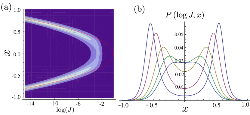
Appendix D Initial Distribution of hoppings

In this Appendix, we derive the form of the initial marginal distribution for all hoppings, $P_{\Gamma=0}\left(J\right)$. The distribution of all bonds connected to single site, say $i$, is

$$P_{\Gamma=0}\left(J\right)=\frac{1}{N}\sum_{j=1}^{N-1}P_{\left|i-j\right|}\left(J_{i}^{j}\right)\delta\left(J-J_{i}^{j}\right),$$ (64)

where $P_{\left|i-j\right|}\left(J_{i}^{j}\right)$ corresponds to the distribution of bonds of a particular length. Note that the left-hand side is independent of $i$. We restrict ourselves to the case where each of the bonds are normally distributed. This assumption is sufficient since, as we have shown in Section IV, all initial distributions of scale-invariant hoppings $G_{i}^{j}$ flow to normal distributions under the RG procedure. Setting $l=\left|i-j\right|$ we have

$$P_{l}\left(J_{i}^{j}\right)=\frac{1}{\sqrt{2\pi\sigma_{l}^{2}}}\exp\left(-\frac{\left(J_{i}^{j}\right)^{2}}{2\sigma_{l}^{2}}\right),$$ (65)

where $\sigma_{l}=\sigma_{0}/l^{\alpha}$. Now we evaluate the approximate form of $P\left(J\right)$ by taking the continuum limit and setting $\sigma_{0}=1$.

$$P\left(J\right) = \frac{1}{N}\int_{0}^{N}dx\frac{1}{\sqrt{2\pi}}\exp\left(-\frac{J^{2}x^{2\alpha}}{2}\right)x^{\alpha},$$ (66)

$$= \frac{1}{N\sqrt{2\pi}}\int_{0}^{N}dx\exp\left(-\frac{J^{2}x^{2\alpha}}{2}+\alpha\ln x\right).$$

We can evaluate Eq. (66) using the saddle point approximation. The saddle point for the function $f\left(x\right)=-\frac{J^{2}x^{2\alpha}}{2}+\alpha\ln x$ is given by the condition $f^{\prime}\left(x^{*}\right)=0$, that is, $x^{*}=J^{-1/\alpha}$. This is a maximum as evidenced by $f^{\prime\prime}\left(x^{*}=J^{-1/\alpha}\right)=-2\alpha^{2}/x^{2}<0$. Now, evaluating Eq. (66) by expanding around the saddle point, we obtain,

$$P\left(J\right) = \frac{\exp\left(-\frac{1}{2}\right)}{N\sqrt{2\pi}J}\int_{0}^{N}dx\exp\left(-2J^{\frac{2}{\alpha}}\alpha^{2}\left(x-J^{-\frac{1}{\alpha}}\right)^{2}\right)$$ (67)

$$\sim \frac{\exp\left(-\frac{1}{2}\right)}{4N\alpha\sqrt{2\pi}J^{1+\frac{1}{\alpha}}},$$

where in the second step we used the limit of large $N$, to approximate $\text{{erf}}\left(N\alpha\sqrt{2}J^{\frac{1}{\alpha}}\right)\approx 1$. Ultimately, the distribution of the bonds becomes

$$P\left(J\right)=\frac{C_{\alpha}}{J^{1+\frac{1}{\alpha}}}.$$ (68)

The validity of the saddle point introduces a finite-size cutoff, dependent on the system size $N$. For the saddle-point approximation to be valid, we require $J^{-1/\alpha}<N$, which means it fails for $J<J_{{\rm c}}\equiv\frac{1}{N^{\alpha}}$. The bonds below $J_{{\rm c}}$ are set to $J=0$. The distribution becomes uniformly distributed since

$$P\left(J\right) \approx \frac{1}{N}\int_{0}^{N}dx\frac{1}{\sqrt{2\pi}}x^{\alpha},$$ (69)

$$= \frac{N^{\alpha}}{\left(\alpha+1\right)\sqrt{2\pi}}.$$

An example of the distribution $P\left(J\right)$ is given in Fig.14, where we consider a site connected to 100 neighbors (average over 70 realizations). Working in log scale, we find the following behavior of $\log P\left(y=\log{x}\right)$,

$$\log P\left(y\right)\sim\begin{cases}y&,y<0\\ -\frac{y}{\alpha}&,y>0\end{cases},$$ (70)

where we have also shifted the distribution (in log scale) so that the crossover point is at $y=0$.

Figure 14: (Color Online) Initial probability distribution $P\left(y=\log{J}\right)$, of couplings connected to an arbitrary test site, in log scale. The distributions have been shifted horizontally so that the maximum of all the curves are located at $y=0$. For $y<0$, the uniform part of the distribution $P\left(J\right)$, corresponding to $\log P\left(y\right)\sim-y$, is independent of $\alpha$. For $y>0$, the angular coefficient, expected to result in $-\frac{1}{\alpha}$, gives $-2.07$ for $\alpha=\frac{1}{2}$ (red line and points), $-1.01$ for $\alpha=1$ (purple line and points), and $-0.51$ for $\alpha=2$ (black line and points). The blue points correspond to $\alpha=0$ , where the saddle point approximation fails.

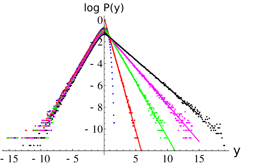
We note that the calculation done here is approximate. The distribution we find is clearly incorrect in the limits of $\alpha\rightarrow 0$ and $\alpha\rightarrow\infty$. In the limit $\alpha\rightarrow 0$, the saddle point calculation is not trustworthy, while in the limit $\alpha\rightarrow\infty$ the continuum approximation done to Eq. (64) is no longer valid.

Appendix E Effect of hoppings on bandwidth

In light of the fact that the power law exponent of the distribution of $J_{i}^{j}$ does not flow for $\alpha>1/2$, we rewrite its evolution as

$$J_{i}^{j}\left(\Gamma\right)=G_{i}^{j}\frac{f_{\Gamma}\left(x_{i}^{j}\right)}{\left|i-j\right|^{\alpha}},$$ (71)

where $G_{i}^{j}$ is a scale-invariant random number and $f_{\Gamma}\left(x_{i}^{j}\right)$ takes into account effects of the $x$ variables into the $J$ evolution. At the starting point, $f_{\Gamma=0}\left(x_{i}^{j}\right)=1$. The equation for the evolution of $f_{\Gamma}\left(x\right)$ follows from Eq. (8),

$$\frac{df_{\Gamma}}{d\Gamma}\left(x\right)=-x^{2}f_{\Gamma}\left(x\right)$$ (72)

whose solution is $f_{\Gamma}\left(x\right)=e^{-\Gamma x^{2}}$. Integrating the evolution of $h_{i}$, Eq. (8), we compute the typical field change $\Delta h_{i}=h_{i}\left(\infty\right)-h_{i}\left(0\right)$, that summarizes the effects of hoppings in the field evolution, and therefore gives the bandwidth

$$\Delta h_{i} \approx N^{1-2\alpha}\frac{1}{2\Gamma}\int^{\frac{1}{N^{\alpha}}}d\Gamma e^{-\Gamma x^{2}}$$ (73)

$$\sim N^{1-2\alpha}\log N.$$ (74)

If $\alpha\leq\frac{1}{2}$, the bandwidth diverges in the thermodynamic limit, while at $\alpha>\frac{1}{2}$ it stays of $\mathcal{O}\left(1\right)$. The logarithmic correction for $\alpha=1/2$ indicates a critical behavior. This is the result quoted in the main text.

Appendix F Strong-bond RG: Details

F.1 RG step derivation.

In this Appendix, we give an outline of some of the derivations used in the main text, in the Strong-bond RG procedure. We start deriving Eqs. (24)-(26). To abbreviate the notation, let us define $c_{i}^{\dagger}\equiv\tilde{i}$ and $c_{i}\equiv i$. We consider the two-site chain, since this is the building block for the RG steps. The idea is to solve this chain in leading order of $\frac{1}{\Gamma}$. The Hamiltonian for three sites is given by

$$H_{3s} = J_{1}^{2}\left(\tilde{1}2+\tilde{2}1\right)+J_{2}^{3}\left(\tilde{2}3+\tilde{3}2\right)+J_{1}^{3}\left(\tilde{1}3+\tilde{3}1\right)$$ (75)

$$+ h_{1}\tilde{1}1+h_{2}\tilde{2}2+h_{3}\tilde{3}3$$

Calculating the generator explicitly, we find

$$\eta = J_{1}^{2}\left(h_{1}-h_{2}\right)\left(\tilde{2}1-\tilde{1}2\right)+J_{2}^{3}\left(h_{2}-h_{3}\right)\left(\tilde{3}2-\tilde{2}3\right)$$ (76)

$$+ J_{1}^{3}\left(h_{1}-h_{3}\right)\left(\tilde{3}1-\tilde{1}3\right)$$

We now make the assumption that $r_{12}\gg r_{23}$. Under this assumption, we consider the evolution in an interval from from $\Gamma=0$ to $\delta\Gamma\sim 1/r_{12}^{2}$ where only bonds and fields related to sites 1 and 2 evolve, while the couplings in other sites change infinitesimally. Keeping the leading order terms (zeroth order in $\delta\Gamma$), we find the evolution of $\eta$ to be

$$\int d\Gamma\eta = \int d\Gamma J_{1}^{2}\left(h_{1}-h_{2}\right)\left(\tilde{2}1-\tilde{1}2\right)+\mathcal{O}\left(\delta\Gamma\right)$$ (77)

$$= \alpha_{12}\left(\tilde{2}1-\tilde{1}2\right)+\mathcal{O}\left(\delta\Gamma\right)$$

where $\alpha_{12}$ was defined in Eq. (21). Higher order corrections can be neglected under the assumption that $\delta\Gamma$ is sufficiently small. Defining $A=\int d\Gamma\eta$ and recalling the Baker-Campbell-Hausdorff formula,

$$e^{A}He^{-A} = H+\left[A,H\right]+\frac{1}{2}\left[A,\left[A,H\right]\right]+\ldots$$ (78)

we find the leading order correction to be

$$\left[H,\alpha_{12}\left(\tilde{2}1-\tilde{1}2\right)\right] = J_{2}^{3}\alpha_{12}\left(\tilde{3}1+1\tilde{3}\right)-J_{1}^{3}\alpha_{12}\left(3\tilde{2}+2\tilde{3}\right).$$ (79)

Therefore, the commutators with the Hamiltonian yield

$$\left[A,H\right] = J_{1}^{3}\alpha_{12}\left(3\tilde{2}+2\tilde{3}\right)-J_{2}^{3}\alpha_{12}\left(\tilde{3}1+1\tilde{3}\right),$$ (80)

$$\left[A,\left[A,H\right]\right] = -J_{2}^{3}\alpha_{12}\left(3\tilde{2}+2\tilde{3}\right)-J_{1}^{2}\alpha_{12}\left(\tilde{3}1+1\tilde{3}\right).$$ (81)

One can easily show, by induction, that summing the series, we find

$$H\left(\delta\Gamma\right) = \left(J_{1}^{3}\cos\alpha_{12}+J_{2}^{3}\sin\alpha_{12}\right)\left(\tilde{3}1+1\tilde{3}\right)$$ (82)

$$+ \left(J_{2}^{3}\cos\alpha_{12}-J_{1}^{3}\sin\alpha_{12}\right)\left(\tilde{3}2+2\tilde{3}\right).$$

and this is the basis for the RG equations (24) and (25). The change in the fields, Eq. (26), can be found with similar reasoning. The generalization for chain of $N$ sites is trivial, since the RG procedure can be thought as processes acting on blocks of three sites.

F.2 Additional numerical results

Numerically, we can compare the spectrum obtained from exact diagonalization and the RG procedure. In Fig. 15, we compare all the single-particle levels from the two methods, obtained for a single disorder realization in a chain of $N=100$ sites. We plot for exponents $\alpha=0.7$, $1.0$, $2.0$ and $5.0$, with Gaussian distribution with unit standard deviation of $h_{i}$ and $G_{i}^{j}$. Clearly we obtain very good agreement between the two procedures in all the cases. The level spacing is more subtle, and studied in the main text.

Figure 15: Comparison of the single particle spectrum obtained from exact-diagonalization with the one obtained from the Strong-bond RG technique. (a)-(d) in ascending order of exponents, $\alpha=0,$ $0.7$, $2.0$, $5.0$. In all cases, both spectra look reasonably similar. A careful inspection of the level-spacing statistics, however, reveals that the eigenvalues obtained in case (a), $\alpha=0$, does not experience repulsion, like a delocalized phase should (see main text for further details about the level spacing).

Appendix G Master Equation

In this appendix, we write down the master equation for the distribution of $J$, $P_{\Gamma}\left(J\right)$, under the RG procedure. We consider the shell in the $J-x$ phase space with radius $r=\sqrt{x^{2}+4J^{2}}$ and width $dr$. We denote the set of all hopping terms by a single variable $J$, and field differences by $x=\left|h_{i}-h_{j}\right|$. Let the distribution of the $x$ in the shell be $n\left(x=r\right)$ and the distribution of the bonds be $P_{\Gamma}\left(J\right)$.

Consider the effects of the decimation of a pair with hopping $J_{i}^{j}$. The $J$ distribution changes due to the removal of a large hopping $J_{i}^{j}$ and by the renormalization of all couplings connected to sites $i$ or $j$. The change in the distribution of the bonds, $\Delta P_{\Gamma}\left(J\right)$, is

$$\Delta P_{\Gamma}\left(J\right)=dr\int_{0}^{2\pi}d\theta_{i}^{j}\int dxdJ_{i}^{j}n\left(x\right)P_{\Gamma}\left(J_{i}^{j}\right)\delta\left(\sqrt{\left(2J_{i}^{j}\right)^{2}+\left(x_{i}^{j}\right)^{2}}-r\right)\int\prod_{k}\left(dJ_{k}^{i}dJ_{k}^{j}\right)P_{\Gamma}\left(J_{k}^{i}\right)P_{\Gamma}\left(J_{k}^{j}\right)\times$$

$$\times\sum_{k}\left[\delta\left(J-\tilde{J}_{k}^{i}\right)+\delta\left(J-\tilde{J}_{k}^{j}\right)-\delta\left(J-J_{k}^{i}\right)-\delta\left(J-J_{k}^{j}\right)-\delta\left(J-J_{i}^{j}\right)\right],$$ (83)

where $\tilde{J}$ variables are defined in the main text, Eqs. (24) and (25) and the angle variable is defined in Eq.( 23). Let us now define

$$\eta\left(r,J_{i}^{j}\right)=\int dxn\left(x\right)\delta\left(\sqrt{\left(2J_{i}^{j}\right)^{2}+x^{2}}-r\right).$$ (84)

We make a simplification $\eta\left(r,J_{i}^{j}\right)\approx\eta\left(r\right)\approx\eta$ , where $\eta$ a constant. This approximation relies on the fact that, for most of the bonds, $J_{i}^{j}\ll x_{i}^{j}$ and so, we approximate $J_{i}^{j}\approx 0$. As the largest $r$-bonds are removed from the chain, the normalization also changes. The number of removed couplings is $\eta dr$ and an overall pre-factor $\left(1-\eta dr\right)^{-1}$ must be included. Therefore, the new distribution $\tilde{P}\left(J\right)$ is given by a sum of the previous distribution $P\left(J\right)$ and the above contribution $\Delta P\left(J\right)$, multiplied by the normalization pre-factor,

$$\tilde{P}\left(J\right) = \frac{1}{1-\eta dr}\left[P\left(J\right)+\eta dr\int d\theta_{i}^{j}\int dJ_{i}^{j}P\left(J_{i}^{j}\right)\int\prod_{k}\left(dJ_{k}^{i}dJ_{k}^{j}\right)\times\right.$$ (85)

$$\times \left.P\left(J_{k}^{i}\right)P\left(J_{k}^{j}\right)\left(\sum_{k,p=i,j}\delta\left(J-\tilde{J}_{k}^{p}\right)+\delta\left(J-J_{k}^{p}\right)-\delta\left(J-J_{i}^{j}\right)\right)\right]$$

$$\implies\tilde{P}\left(J\right) = P\left(J\right)+\eta dr\int dJ_{i}^{j}P\left(J_{i}^{j}\right)\int\prod_{k}dJ_{k}^{i}dJ_{k}^{j}P\left(J_{k}^{i}\right)P\left(J_{k}^{j}\right)\sum_{k}\left(\sum_{p=\left\{i,j\right\}}\delta\left(J-\tilde{J}_{k}^{p}\right)-\delta\left(J-J_{k}^{p}\right)\right)$$

For simplicity we assume $n\left(r\right)$ to be a constant. We now take the continuum limit as the scale $r$ reduces. The master equation becomes

$$\frac{\partial P\left(J\right)}{\partial r}=\eta\int d\theta_{i}^{j}\int dJ_{i}^{j}P\left(J_{i}^{j}\right)\int\prod_{k}dJ_{k}^{i}dJ_{k}^{j}P\left(J_{k}^{i}\right)P\left(J_{k}^{j}\right)\sum_{k}\left(\sum_{p=\left\{i,j\right\}}\delta\left(J-\tilde{J}_{k}^{p}\right)-\delta\left(J-J_{k}^{p}\right)\right).$$

Notice that this equation keeps track of how the distribution changes with $r$, not with the scale $\Gamma$. In the main text, we take alternative routes using physical arguments in order to find the fixed point distribution, instead of directly solving this full master equation.

Appendix H Wavefunction and IPR from RG

In this appendix, we discuss the properties of the eigenfunctions obtained from the RG procedure. The RG procedure consists of a rotation of the basis states at each decimation step. Let the set of eigenfunctions of the Hamiltonian be $\psi_{E}\left(i\right)$, where $i$ denotes the site index and $E$ the eigenfunction label. We define a function for the intermediate RG steps, $\psi_{E}^{m}\left(i\right)$, where $m$ denotes the decimation step. The initial condition before any decimation steps is $\psi_{E}^{0}\left(i\right)=\delta_{i,E}$, that is, completely localized in position space. The eigenfunctions from the RG procedure are obtained at the end of all the steps. We call these final functions $\psi_{E}^{F}\left(i\right)$. Now, consider at a particular decimation step, $m$, where the bond between sites $\left(i,j\right)$ is decimated. As discussed in Section IV, the corresponding rotation angle, $\alpha_{ij}$ was defined in Eq. (21). In this step, all the intermediate functions $\psi_{E}^{m}\left(i\right)$ are modified according to

$$\psi_{E}^{m+1}\left(i\right) = \cos\left(\alpha_{ij}\right)\psi_{E}^{m}\left(i\right)+\sin\left(\alpha_{ij}\right)\psi_{E}^{m}\left(j\right),$$ (86)

$$\psi_{E}^{m+1}\left(j\right) = -\sin\left(\alpha_{ij}\right)\psi_{E}^{m}\left(i\right)+\cos\left(\alpha_{ij}\right)\psi_{E}^{m}\left(j\right).$$ (87)

From this procedure, we can obtain the value of the IPR, by collecting the final wave functions and computing

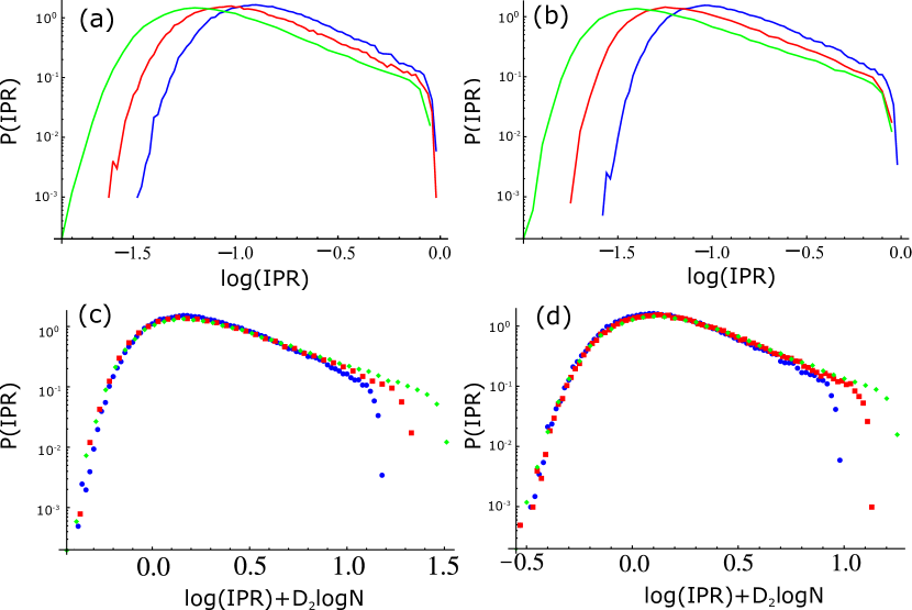
$$\mbox{IPR}=\sum_{i,E}\left|\psi_{E}^{F}\left(i\right)\right|^{4}$$ (88)

The IPR scales as $L^{-D_{2}}$ where $D_{2}=0$ for localized states and $D_{2}=d$ (where $d$ is the system dimension) for the extended states [8]. For critical states [26, 8], $0<D_{2}<d$. Furthermore, at the critical point, the IPR distribution is postulated to only shift and not change shape as a function of system size. We can obtain a scaling collapse by making the appropriate rescaling, $\log\mbox{IPR}\rightarrow\log\mbox{IPR}+D_{2}\log N$. We plot the comparison of the IPR, at $\alpha=1$, obtained from the RG procedure and exact diagonalization in the Fig. 16, with the scaling collapses as insets. The IPR obtained from the RG reproduces the critical behavior, with $D_{2}=0.5$ for the RG case and $D_{2}=0.6$ for exact diagonalization.

Figure 16: Finite size scaling of the IPR for different system sizes $N=100$ (blue), $N=200$ (red) and $N=400$ (green). The finite size dependence and scaling collapse are shown in (a) and (c) for the proposed RG procedure, and (b) and (d) for exact diagonalization respectively. The data are taken for the critical point, $\alpha=1$ The initial distributions of $G_{i}^{j}$ and $h_{i}$ are Gaussian. The fractal dimensions are found from the scaling $\log\mbox{IPR}\rightarrow\log\mbox{IPR}+D_{2}\log N$. We find $D_{2}=0.5$ for the RG case (a), and $D_{2}=0.6$ for the case of exact diagonalization (b).

References

- Anderson [1958] P. W. Anderson, Phys. Rev. 109, 1492 (1958).
- Evers and Mirlin [2008] F. Evers and A. D. Mirlin, Rev. Mod. Phys. 80, 1355 (2008).
- Kramer and MacKinnon [1993] B. Kramer and A. MacKinnon, Reports on Progress in Physics 56, 1469 (1993).
- Abrahams et al. [1979] E. Abrahams, P. W. Anderson, D. C. Licciardello, and T. V. Ramakrishnan, Phys. Rev. Lett. 42, 673 (1979).
- Gruzberg et al. [2011] I. A. Gruzberg, A. W. W. Ludwig, A. D. Mirlin, and M. R. Zirnbauer, Phys. Rev. Lett. 107, 086403 (2011).
- Levitov [1990] L. S. Levitov, Phys. Rev. Lett. 64, 547 (1990).
- Mirlin et al. [1996] A. D. Mirlin, Y. V. Fyodorov, F.-M. Dittes, J. Quezada, and T. H. Seligman, Phys. Rev. E 54, 3221 (1996).
- Evers and Mirlin [2000] F. Evers and A. D. Mirlin, Phys. Rev. Lett. 84, 3690 (2000).
- Basko et al. [2006] D. Basko, I. Aleiner, and B. Altshuler, Annals of Physics 321, 1126 (2006).
- Bardarson et al. [2012] J. H. Bardarson, F. Pollmann, and J. E. Moore, Phys. Rev. Lett. 109, 017202 (2012).
- Pekker et al. [2014] D. Pekker, G. Refael, E. Altman, E. Demler, and V. Oganesyan, Phys. Rev. X 4, 011052 (2014).
- Huse et al. [2014] D. A. Huse, R. Nandkishore, and V. Oganesyan, Phys. Rev. B 90, 174202 (2014).
- Vosk et al. [2015] R. Vosk, D. A. Huse, and E. Altman, Phys. Rev. X 5, 031032 (2015).
- Schreiber et al. [2015] M. Schreiber, S. S. Hodgman, P. Bordia, H. P. Lüschen, M. H. Fischer, R. Vosk, E. Altman, U. Schneider, and I. Bloch, Science 349, 842 (2015).
- Luitz et al. [2015] D. J. Luitz, N. Laflorencie, and F. Alet, Phys. Rev. B 91, 081103 (2015).
- Rademaker and Ortuño [2016] L. Rademaker and M. Ortuño, Phys. Rev. Lett. 116, 010404 (2016).
- Vasseur et al. [2015] R. Vasseur, A. C. Potter, and S. A. Parameswaran, Phys. Rev. Lett. 114, 217201 (2015).
- Pal and Huse [2010] A. Pal and D. A. Huse, Phys. Rev. B 82, 174411 (2010).
- Oganesyan and Huse [2007] V. Oganesyan and D. A. Huse, Phys. Rev. B 75, 155111 (2007).
- Monthus [2016a] C. Monthus, arXiv preprint arXiv:1602.03064 (2016a).
- Serbyn and Moore [2016] M. Serbyn and J. E. Moore, Phys. Rev. B 93, 041424 (2016).
- Kravtsov et al. [2015] V. E. Kravtsov, I. M. Khaymovich, E. Cuevas, and M. Amini, New Journal of Physics 17, 122002 (2015).
- Monthus [2016b] C. Monthus, arXiv preprint arXiv:1603.04701 (2016b).
- Monthus [2016c] C. Monthus, Entropy 18, 122 (2016c).
- Monthus [2016d] C. Monthus, Journal of Statistical Mechanics: Theory and Experiment 2016, 033113 (2016d).
- Shklovskii et al. [1993] B. I. Shklovskii, B. Shapiro, B. R. Sears, P. Lambrianides, and H. B. Shore, Phys. Rev. B 47, 11487 (1993).
- Avishai et al. [2002] Y. Avishai, J. Richert, and R. Berkovits, Phys. Rev. B 66, 052416 (2002).
- Santos [2004] L. F. Santos, Journal of Physics A: Mathematical and General 37, 4723 (2004).
- Ma et al. [1979] S. k. Ma, C. Dasgupta, and C. k. Hu, Phys. Rev. Lett. 43, 1434 (1979).
- C. Dasgupta and S.-k. Ma [1980] C. Dasgupta and S.-k. Ma, Phys. Rev. B 22, 1305 (1980).
- Agarwal et al. [2015] K. Agarwal, E. Demler, and I. Martin, Phys. Rev. B 92, 184203 (2015).
- You et al. [2016] Y.-Z. You, X.-L. Qi, and C. Xu, Phys. Rev. B 93, 104205 (2016).
- Wegner [1994] F. Wegner, Ann. Physik 3, 77 (1994).
- Głazek and Wilson [1993] S. D. Głazek and K. G. Wilson, Phys. Rev. D 48, 5863 (1993).
- Glazek and Wilson [1994] S. D. Glazek and K. G. Wilson, Phys. Rev. D 49, 4214 (1994).
- Levitov [1989] L. S. Levitov, EPL (Europhysics Letters) 9, 83 (1989).
- Javan Mard et al. [2014] H. Javan Mard, J. A. Hoyos, E. Miranda, and V. Dobrosavljević, Phys. Rev. B 90, 125141 (2014).
- Mirlin and Evers [2000] A. D. Mirlin and F. Evers, Phys. Rev. B 62, 7920 (2000).
- Mehta [2004] M. L. Mehta, Random Matrices (Academic Press, 2004).
- Beenakker [1997] C. W. J. Beenakker, Rev. Mod. Phys. 69, 731 (1997).
- Kehrein [2006] S. Kehrein, The Flow Equation Approach to Many-Particle Systems (Springer-Verlag Berlin Heidelberg, 2006).
- Golub and Loan [2012] G. H. Golub and C. F. V. Loan, Matrix Computations (Johns Hopkins University Press, 2012).
- Wigner [1951] E. P. Wigner, Ann. of Math. 53, 36 (1951).
- de Monvel et al. [1995] A. de Monvel, L. Pastur, and M. Shcherbina, Journal of Statistical Physics 79, 585 (1995).
- Serbyn et al. [2013] M. Serbyn, Z. Papić, and D. A. Abanin, Phys. Rev. Lett. 111, 127201 (2013).
- Pekker et al. [2016] D. Pekker, B. K. Clark, V. Oganesyan, and G. Refael, arXiv preprint arXiv:1607.07884 (2016).
- Khatami et al. [2012] E. Khatami, M. Rigol, A. Relaño, and A. M. García-García, Phys. Rev. E 85, 050102 (2012).