Reconstruction and stability for piecewise smooth potentials in the plane

Abstract.

We show that complex-valued potentials with jump discontinuities can be recovered from the Dirichlet-to-Neumann map using Bukhgeim’s method. Combining with known formulas, this enables the recovery from the scattering amplitude at a fixed energy. We also provide a priori stability estimates for reconstruction from the Dirichlet ​​-to-Neumann map as well as from the scattering amplitude given an approximate knowledge of the location of the discontinuities.

1. Introduction

Let $\Omega$ be a bounded planar domain that contains a bounded potential $V$, and consider the Dirichlet problem

(1) $$\left\{\begin{array}[]{l}\Delta u=Vu\\ u|_{\partial\Omega}=f.\end{array}\right.$$

Supposing that 0 is not a Dirichlet eigenvalue, there is a unique solution $u\in H^{1}(\Omega)$ and the DtN map $\Lambda_{V}$ can be formally defined by

$$\Lambda_{V}:f\rightarrow\nabla u\cdot\mathbf{n}|_{\partial\Omega}.$$

Our goal is then to recover the potential from the information contained in $\Lambda_{V}$. This problem has a long history and is closely related to the inverse conductivity problem proposed by Calderón; see [14]. Some relevant work in higher dimensions includes [34, 27, 29, 11, 25, 22, 21, 16].

The two dimensional question is quite different to the higher dimensional case; for example the inverse problem is no longer overdetermined. In [28] Nachman introduced the $\overline{\partial}$-method to prove uniqueness for conductivities in $W^{2,p}$ with $p>1$, and gave a reconstruction procedure (this work has since been extended to more general cases, see for example [23, 12]). In [7], combining the $\overline{\partial}$-method with the theory of quasi-conformal maps, Astala and Päivärinta solved the uniqueness problem for $L^{\infty}$ conductivities.

There was little progress for general potentials in the plane until Bukhgeim introduced a new method, proving uniqueness for $C^{1}$-potentials [13]. There he took advantage of solutions of the form

$$u=u_{\lambda,x}=e^{i\lambda\psi}(1+w),\quad\psi(z)=\psi_{x}(z)=\frac{1}{2}\big{(}z_{1}-x_{1}+i(z_{2}-x_{2})\big{)}^{2},$$

where $w=w_{\lambda,x}$ is small in some sense. Indeed, after proving that the the integral

$$\int_{\Omega}e^{i\lambda(\psi+\overline{\psi})}\,V\,w$$

converges to zero as $\lambda$ grows, one uses the stationary phase method to see that the integral

$$\int_{\partial\Omega}e^{i\lambda\overline{\psi}}(\Lambda_{V}-\Lambda_{0})[u]=\int_{\Omega}e^{i\lambda(\psi+\overline{\psi})}\,V\,(1+w)$$

converges to $\pi\lambda^{-1}V(x)$.

This quadratic phase approach has since been extended by many authors; we list a few here. Novikov and Santacesaria obtained stability estimates for $C^{2}$-potentials in [30] and proved that the reconstruction method could be extended to $C^{1}$ matrix-valued potentials in [31]. In [10], Blåsten, Imanuvilov and Yamamoto proved uniqueness for potentials in $L^{p}$ with $p>2$, and gave stability estimates in the $L^{2}$ norm for potentials in $H^{s}$ with $s>0$. Finally, Astala, Faraco and Rogers gave a reconstruction procedure for potentials in $H^{1/2}$ and proved that this is best possible in some sense; see [4].

In the recent work [26], Lakshtanov, Novikov and Vainberg provided a reconstruction scheme for real bounded potentials. Their procedure relies on Faddeev’s scattering solutions and allows to recover almost each potential, in the sense of their Remark 4.1.

Here we will prove that the reconstruction formula given in [4] (mildly different from the original Bukhgeim formula) works for piecewise $W^{2,1}$-potentials with jump discontinuities on smooth curves. That is to say potentials $V$ that can be written as

$$V(x)=\sum_{j=1}^{N}q_{j}(x)\raisebox{2.0pt}{$\chi$}_{\Omega_{j}}(x),$$

where $q_{j}\in W^{2,1}(\Omega_{j})$ and $\Omega_{j}$ are piecewise $C^{2,\alpha}$-domains with $\alpha>1/2$. By this we mean, the boundary $\partial\Omega_{j}$ can be expressed as a finite union of graphs of $C^{2,\alpha}$-functions and that the union is Lipschitz. The most significant novelties of the article are to be found in Section 3, where we will prove the following theorem. There we will also present a potential for which the recovery formula fails at points away from the discontinuities.

Theorem 1.1.

Let $V$ be a piecewise $W^{2,1}$-potential with jump discontinuities on smooth curves. Then

$$\lim_{\lambda\rightarrow\infty}\frac{\lambda}{\pi}\int_{\partial\Omega}e^{i\lambda\overline{\psi}}\left(\Lambda_{V}-\Lambda_{0}\right)\left[u_{\lambda,x}\right]=V(x),\quad\text{a.e.}\ x\in\Omega.$$

We refer to Theorem 1.1 of [4] for how to determine the values of the Bukhgeim solutions on the boundary.

For a fixed $k>0$, we also consider the Schrödinger equation

(2) $$(-\Delta+V)u=k^{2}u,$$

where $k^{2}$ is not a Dirichlet eigenvalue for the Hamiltonian $-\Delta+V$. For $\theta\in\mathbb{S}^{1}$, the outgoing scattering solutions satisfy the Lippmann-Schwinger equation

$$u(x,\theta)=e^{ikx\cdot\theta}-\int_{\mathbb{R}^{2}}G_{0}(x,y)V(y)u(y,\theta)\,dy,$$

where $G_{0}$ denotes the outgoing Green’s function which satisfies

$$(-\Delta-k^{2})G_{0}(x,y)=\delta(x-y).$$

Then the scattering amplitude $A_{V}:\mathbb{S}^{1}\times\mathbb{S}^{1}\rightarrow\mathbb{C}$ at energy $k^{2}$ can be written

$$A_{V}(\eta,\theta)=\int_{\mathbb{R}^{2}}e^{-ik\eta\cdot y}V(y)u(y,\theta)\,dy.$$

Given an incident plane wave in direction $\theta$, the scattering amplitude measures the probability of scattering in the direction $\eta$. A classical problem is to recover the potential in (2) from the information contained in $A_{V}$.

By applying the formula obtained in [5], we can also recover $V$ from $A_{V}$ as long as $V$ is a piecewise $W^{2,1}$-potential with jump discontinuities on smooth curves. More details will be given in the third section.

Stability estimates are a classical theme in inverse problems; see [3, 10] for the Schrödinger equation and [2, 8, 9, 17, 15] for the conductivity equation. Notice that in [10] or in [17] there is stability for discontinuous potentials or conductivities but only in the $L^{2}$ sense. A careful analysis of the dependence of the constants in the reconstruction theorem yields an $L^{\infty}$ stability for discontinuous coefficients provided a noise knowledge of the discontinuities of the potential. In the final section we will prove stability estimates for the reconstruction from the DtN map and from the information contained in $A_{V}$.

2. Preliminaries

2.1. Quadratic phase solutions and integrals

Using Wirtinger derivatives we can write the the time-independent Schrödinger equation as $4\partial_{z}\partial_{\overline{z}}u=Vu$. Taking solutions of the form $u=e^{i\lambda\psi}(1+w)$ and multiplying both sides by $e^{i\lambda\overline{\psi}}$ we obtain

$$4e^{i\lambda\overline{\psi}}\partial_{z}\partial_{\overline{z}}e^{i\lambda\psi}(1+w)=e^{i\lambda(\psi+\overline{\psi})}V(1+w).$$

Taking into account that $\partial_{\overline{z}}e^{i\lambda\psi}=\partial_{z}e^{i\lambda\overline{\psi}}=0$, this can be rewritten as

$$4\partial_{z}e^{i\lambda(\psi+\overline{\psi})}\partial_{\overline{z}}w=e^{i\lambda(\psi+\overline{\psi})}V(1+w).$$

As the derivatives are local operators, and we need only satisfying the equation inside $\Omega$, we can take solutions of the form

$$w=\frac{1}{4}\partial_{\overline{z}}^{-1}\left[e^{-i\lambda(\psi+\overline{\psi})}\,\raisebox{2.0pt}{$\chi$}_{Q}\,\partial_{z}^{-1}\left[e^{i\lambda(\psi+\overline{\psi})}\,\raisebox{2.0pt}{$\chi$}_{Q}\,V\,(1+w)\right]\right]$$

where $Q$ is an auxiliary axis-parallel square containing $\Omega$. In order to simplify notation we define the multiplication operators

$$M^{\pm\lambda}\left[F\right]=e^{\pm i\lambda(\psi+\overline{\psi})}\raisebox{2.0pt}{$\chi$}_{Q}F,$$

and write

$$S^{\lambda}_{1}\left[F\right]=\frac{1}{4}\partial^{-1}_{\overline{z}}\circ M^{-\lambda}\circ\partial^{-1}_{z}\circ M^{\lambda},\quad S^{\lambda}_{V}\left[F\right]=S^{\lambda}_{1}\left[VF\right].$$

For sufficiently smooth $V$, the operator norm of $S^{\lambda}_{V}$ is small for large enough $\lambda$; see [4, Lemma 2.3], so we can invert $(I-S^{\lambda}_{V})$ using Neumann series, yielding

$$w=w_{\lambda,x}=(I-S^{\lambda}_{V})^{-1}S^{\lambda}_{1}\left[V\right].$$

The following oscillatory integral operator will also be useful in the sequel

$$T^{\lambda}_{w}[F](x)=\frac{\lambda}{\pi}\int_{\mathbb{R}^{2}}e^{i\lambda(\psi+\overline{\psi})}F(z)w_{\lambda,x}(z)\,dz.$$

In order to study the behaviour of these operators we will use the homogeneous $L^{2}$ Sobolev space, denoted by $\dot{H}^{s}$, with norm $\left\|f\right\|_{\dot{H}^{s}}=\||\cdot|^{s}\hat{f}\|_{L^{2}},$ where $\hat{f}$ is the Fourier transform of $f$.

We have the following bound for $M^{\pm\lambda}$; the proof can be found in [4, Section 2]. The key ingredient in the proof is the classical lemma of van der Corput.

Lemma 2.1.

Let $0\leq s_{1},s_{2}<1$. Then

$$\left\|M^{\pm\lambda}[F]\right\|_{\dot{H}^{-s_{2}}}\leq C\lambda^{-\min\{s_{1},s_{2}\}}\left\|F\right\|_{\dot{H}^{s_{1}}},\quad\lambda\geq 1.$$

The following two lemmas were essentially proven in [4, Sections 2 and 4]; we present minor modifications, suitable for the stability analysis of the final section.

Lemma 2.2.

Let $0<s_{1},s_{2}<1$. Then there exists a constant $C$ such that

$$\left\|S^{\lambda}_{1}\right\|_{\dot{H}^{s_{1}}\rightarrow\dot{H}^{s_{2}}}\leq\,C\,\lambda^{-\tau}$$

where $\tau=1-s_{2}+\min\{s_{1},s_{2}\}$.

Proof.

Using Lemma 2.1 twice we get

$$\left\|S^{\lambda}_{1}\right\|_{\dot{H}^{s_{1}}\rightarrow\dot{H}^{s_{2}}} \leq \left\|M^{-\lambda}\circ\partial_{z}^{-1}\circ M^{\lambda}\right\|_{\dot{H}^{s_{1}}\rightarrow\dot{H}^{s_{2}-1}}$$

$$\leq C\,\lambda^{-1+s_{2}}\left\|\partial_{z}^{-1}\circ M^{\lambda}\right\|_{\dot{H}^{s_{1}}\rightarrow\dot{H}^{1-s_{2}}}$$

$$\leq C\,\lambda^{-1+s_{2}}\left\|M^{\lambda}\right\|_{\dot{H}^{s_{1}}\rightarrow\dot{H}^{-s_{2}}}$$

$$\leq C\,\lambda^{-\tau},$$

and the proof is concluded. ∎

Lemma 2.3.

Let $F,V\in\dot{H}^{s}$ where $0<s<1$. Then there exists a constant $C$ such that

$$\sup_{x\in\Omega}\left|T^{\lambda}_{w}[F](x)\right|\leq C\lambda^{-s}\left\|F\right\|_{\dot{H}^{s}}\left\|V\right\|_{\dot{H}^{s}}$$

when $\lambda$ is sufficiently large.

Proof.

Using Lemma 2.1 we obtain

$$\left|T^{\lambda}_{w}[F](x)\right| \leq C\,\lambda\left\|M^{\lambda}[F]\right\|_{\dot{H}^{-s}}\left\|w\right\|_{\dot{H}^{s}}$$

$$\leq C\,\lambda^{1-s}\left\|F\right\|_{\dot{H}^{s}}\left\|(I-S_{V}^{\lambda})^{-1}S_{1}^{\lambda}[V]\right\|_{\dot{H}^{s}}.$$

As $(I-S_{V}^{\lambda})^{-1}$ is bounded for $\lambda$ sufficiently large (see [4, Lemma 2.3]),

$$\left|T^{\lambda}_{w}[F](x)\right| \leq C\lambda^{1-s}\left\|F\right\|_{\dot{H}^{s}}\left\|S_{1}^{\lambda}[V]\right\|_{\dot{H}^{s}}$$

$$\leq C\lambda^{-s}\left\|F\right\|_{\dot{H}^{s}}\left\|V\right\|_{\dot{H}^{s}},$$

where the last inequality comes from applying Lemma 2.2. ∎

Let $g:\mathbb{R}\rightarrow\mathbb{R}\in C^{n}$. We say that $x_{s}$ is a stationary point of $g$ of order $m<n$ if $g^{(k)}(x_{s})=0$ for $1\leq k\leq m$ and $g^{(m+1)}(x_{s})\neq 0$. We say that $g$ has stationary points if such points exist. The following lemma describes the asymptotic behaviour of a one dimensional oscillatory integral with a $C^{2}$ phase when there are only a finite number of stationary points of order one.

Lemma 2.4.

Let $h\in W^{1,1}([a,b])$ and $g\in C^{2}([a,b])$ be such that $g$ has only a finite number of stationary points of order at most one. Then there exists a constant $C$, independent of $h$ and depending continuously on the $C^{2}$ norm of $g$, such that

$$\left|\int_{a}^{b}e^{i\lambda g(x)}h(x)dx\right|\leq C\lambda^{-1/2}\left\|h\right\|_{W^{1,1}([a,b])}$$

for $\lambda>1$.

Proof.

Let $\{s_{j}\}_{j=1}^{N}$ denote the stationary points and $\delta=\min_{j}(|g^{\prime\prime}(s_{j})|)$. Let $\epsilon$ be such that $|g^{\prime\prime}(x)|>\delta/2$ for all $x\in\cup_{j}U_{j}$, where $U_{j}=(u_{j}^{d},u_{j}^{u})=B_{\epsilon}(s_{j})\cap[a,b]$. Then we can make use of a version of Van der Corput’s lemma (see [20, Corollary 2.6.8]), to obtain

$$\left|\int_{U_{j}}e^{i\lambda g(x)}h(x)dx\right|\leq 24\left(\frac{\delta}{2}\right)^{-1/2}\lambda^{-1/2}\left(\left|h(u_{j}^{u})\right|+\int_{U_{j}}\left|h^{\prime}(x)\right|dx\right).$$

Now let $V_{j}=(v_{j}^{d},v_{j}^{u})$ denote each of the remaining segments of $[a,b]$, such that $\cup_{j}V_{j}=[a,b]\setminus\cup_{j}U_{j}$. Integrating by parts in each $V_{j}$ we obtain

$$\int_{V_{j}}e^{i\lambda g(x)}h(x)dx = \frac{1}{i\lambda}\left[\frac{e^{i\lambda g(x)}h(x)}{g^{\prime}(x)}\right]_{v_{j}^{d}}^{v_{j}^{u}}$$

$$-\frac{1}{i\lambda}\int_{V_{j}}e^{i\lambda g(x)}\frac{d}{dx}\left(\frac{h(x)}{g^{\prime}(x)}\right)dx.$$

By Sobolev embedding [1, Theorem 4.12, Part 1, Case A] we have that $\left\|h\right\|_{L^{\infty}[a,b]}\leq C\left\|h\right\|_{W^{1,1}[a,b]}$. Making use of this and Hölder’s inequality, altogether we obtain

$$\left|\int_{a}^{b}e^{i\lambda g(x)}h(x)dx\right| \leq 48N\left(\frac{\delta}{2}\right)^{-1/2}\lambda^{-1/2}\left\|h\right\|_{W^{1,1}([a,b])}$$

$$+(N+1)\ \kappa\,\lambda^{-1}\left\|h\right\|_{W^{1,1}([a,b])},$$

where

$$\kappa=\max_{j}\left\{2\left\|(g^{\prime})^{-1}\right\|_{L^{\infty}(V_{j})}+\left\|\frac{g^{\prime}-g^{\prime\prime}}{(g^{\prime})^{2}}\right\|_{L^{\infty}(V_{j})}\right\},$$

which is finite, as there are no stationary points in $\cup_{j}V_{j}$. For $\lambda>1$ we can take

$$C=48N\left(\frac{\delta}{2}\right)^{-1/2}+(N+1)\,\kappa.$$

As $\delta$ and $\kappa$ depend continuously on the $C^{2}$ norm of $g$, the proof is concluded. ∎

2.2. Piecewise $W^{s,1}$-potentials

We say that a curve $\mathcal{C}$ in the plane is contained in $C^{m,\alpha}$, with $m\geq 0$ and $0\leq\alpha\leq 1$, if there exists a finite collection of bounded open sets $\{U_{j}\}_{j=1}^{N}$ such that $\mathcal{C}\subset\cup_{j=1}^{N}U_{j}$, and functions $f_{j}\in C^{m,\alpha}(\mathbb{R})$ such that

$$\mathcal{C}\cap U_{j}\subset\{(x,f_{j}(x))\,:\,x\in\mathbb{R}\}\quad\text{or}\quad\mathcal{C}\cap U_{j}\subset\{(f_{j}(y),y)\,:\,y\in\mathbb{R}\}.$$

For $\alpha=0$, we write $f\in C^{m,0}(\mathbb{R})$ whenever $f$ and its derivatives up to order $m$ are continuous and bounded; occasionally we will describe the curve as being simply $C^{m}$.

Consider two curves $\mathcal{C}_{1}$ and $\mathcal{C}_{2}$ for which there is a finite cover by open sets $\{U_{j}\}_{j=1}^{N}$ such that for each $j$ either

$$\mathcal{C}_{1}\cap U_{j}\subset\{(x,f_{1,j}(x))\,:\,x\in\mathbb{R}\}\quad\text{and}\quad\mathcal{C}_{2}\cap U_{j}\subset\{(x,f_{2,j}(x))\,:\,x\in\mathbb{R}\}$$

or

$$\mathcal{C}_{1}\cap U_{j}\subset\{(f_{1,j}(y),y)\,:\,y\in\mathbb{R}\}\quad\text{and}\quad\mathcal{C}_{2}\cap U_{j}\subset\{(f_{2,j}(y),y)\,:\,y\in\mathbb{R}\}.$$

Then we define the distance between the two curves in $C^{m,\alpha}$ norm as

$$d(\mathcal{C}_{1},\mathcal{C}_{2})=\inf\left\{\sup_{j}\left\{\left\|f_{1,j}-f_{2,j}\right\|_{C^{m,\alpha}}\right\}\right\}$$

where the infimum is taken over all possible common covers. If a common cover does not exists for the curves, we write $d(\mathcal{C}_{1},\mathcal{C}_{2})=\infty$.

A bounded Lipschitz domain whose boundary is a finite union of $C^{m,\alpha}$ curves will be referred to as a piecewise $C^{m,\alpha}$ domain. The potentials that we will consider exhibit discontinuities over $C^{2,\alpha}$ curves, where $1/2<\alpha\leq 1$. More precisely, we are concerned with piecewise $W^{s,1}$-potentials $V$ that can be expressed as

$$V(x)=\sum_{j=1}^{N}q_{j}(x)\raisebox{2.0pt}{$\chi$}_{\Omega_{j}}(x),$$

where $q_{j}\in W^{s,1}(\mathbb{R}^{2})$ and $\Omega_{j}$ are piecewise $C^{2,\alpha}$ domains with $1/2<\alpha\leq 1$. We will use the following norm for these potentials:

$$\left\|V\right\|_{D^{s,r}}=\inf\left\{\sum_{j=1}^{N}\left\|q_{j}\right\|_{W^{s,1}}\left(1+\left\|\raisebox{2.0pt}{$\chi$}_{\Omega_{j}}\right\|_{H^{r}}\right):V(x)=\sum_{j=1}^{N}q_{j}(x)\raisebox{2.0pt}{$\chi$}_{\Omega_{j}}(x)\right\}$$

where $q_{j}$ and $\Omega_{j}$ are as previously described.

The following lemma provides a bound for the $L^{2}$ Sobolev norm for the potentials of our interest.

Lemma 2.5.

Let $q:\mathbb{R}^{2}\rightarrow\mathbb{R}$ and let $\Omega$ be a bounded Lipschitz domain in the plane. Then there exists a constant $C$ independent of $q$ and $\Omega$ such that

i) For $0<r$ we have

$$\left\|q\right\|_{H^{r}}\leq C\left\|q\right\|_{W^{r+1,1}}.$$

ii) For $0<r<1/2$ we have

$$\left\|q\,\raisebox{2.0pt}{$\chi$}_{\Omega}\right\|_{H^{r}}\leq C\left\|q\,\raisebox{2.0pt}{$\chi$}_{\Omega}\right\|_{D^{2,r}}.$$

Proof.

Let $m$ be the largest integer less than $r$, let $t=r-m$ and let $D^{t}=\leavevmode\nobreak\ (-\Delta)^{t/2}$. For the first case we can use Sobolev embedding; see for example [1, Theorem 4.12, Part 1, Case C], and the fact that $W^{r+1,1}\hookrightarrow W^{m+1,1}$ to obtain

$$\left\|q\right\|_{H^{r}} \leq \left(\left\|q\right\|_{H^{m}}^{2}+\left\|D^{t}q\right\|_{H^{m}}^{2}\right)^{1/2}\leq C\left(\left\|q\right\|_{H^{m}}^{2}+\left\|D^{t}q\right\|_{W^{m+1,1}}^{2}\right)^{1/2}$$

$$\leq C\left(\left\|q\right\|_{H^{m}}^{2}+\left\|q\right\|_{W^{r+1,1}}^{2}\right)^{1/2}\leq C\left\|q\right\|_{W^{r+1,1}}.$$

For the second case we can use the generalised Leibniz rule [24, Theorem A.12], which states that

$$\left\|D^{r}(q\,\raisebox{2.0pt}{$\chi$}_{\Omega})-q\,D^{r}(\raisebox{2.0pt}{$\chi$}_{\Omega})-\raisebox{2.0pt}{$\chi$}_{\Omega}\,D^{r}(q)\right\|_{L^{2}}\leq C\left\|q\right\|_{L^{\infty}}\left\|D^{r}(\raisebox{2.0pt}{$\chi$}_{\Omega})\right\|_{L^{2}},$$

and so by triangle inequality we obtain

(3) $$\left\|q\,\raisebox{2.0pt}{$\chi$}_{\Omega}\right\|_{H^{r}}\leq C\left(\left\|q\right\|_{L^{\infty}}\left\|\raisebox{2.0pt}{$\chi$}_{\Omega}\right\|_{H^{r}}+\left\|q\right\|_{H^{r}}\left\|\raisebox{2.0pt}{$\chi$}_{\Omega}\right\|_{L^{\infty}}\right).$$

For the first term in the right-hand side, we can use Sobolev embedding; see for example [1, Theorem 4.12, Part 1, Case A], to obtain

$$\left\|q\right\|_{L^{\infty}}\leq C\left\|q\right\|_{W^{2,1}}.$$

On the other hand, we have $\raisebox{2.0pt}{$\chi$}_{\Omega}\in H^{r}$ for $r<1/2$; see for example [19]. For the second term in the right-hand side of (3) we can use case $i)$, combined with the embedding $W^{2,1}\hookrightarrow W^{1+r,1}$, concluding the proof. ∎

2.3. A topological property of $C^{1}$ graphs

Finally, we provide a simple continuity result that will be useful for characterizing the topological properties of the set of points where the reconstruction is not guaranteed as well as the continuity properties of the error bound of the reconstruction.

Lemma 2.6.

Let $f\in C^{1}[a,b]$ and $\{x_{j}\}_{j=1}^{N}\in(a,b)$ be such that $f(x_{j})=0$, $f^{\prime}(x_{j})\neq 0$ and $f(x)\neq 0$ for all $x\in[a,b]\setminus\{x_{j}\}_{j=1}^{N}$. Then, for any $\epsilon>0$, there exists $\delta$ such that if $\left\|f-g\right\|_{C^{1}}<\delta$ then there exists $\{x_{j}^{*}\}_{j=1}^{N}\in(a,b)$ such that

$$|x_{j}-x_{j}^{*}|<\epsilon,$$

with $g(x_{j}^{*})=0$, $g^{\prime}(x_{j}^{*})\neq 0$ and $g(x)\neq 0$ for all $x\in[a,b]\setminus\{x_{j}^{*}\}_{j=1}^{N}$.

Proof.

Let $\eta=\min_{j}\{|f^{\prime}(x_{j})|\}$ and let $r$ be such that $|f^{\prime}(x)|>\eta/2$ for all $x\in\cup B_{r}(x_{j})$. Let

$$a=\inf_{x\in[a,b]\setminus\cup B_{r}(x_{j})}\{|f(x)|\}.$$

Then, for all $g$ such that

$$\left\|f-g\right\|_{C^{1}}<\tfrac{1}{2}\min\{a,\eta/2\},$$

we have

$$|g(x)|>a/2,\quad\forall\ x\in[a,b]\setminus\cup_{j}B_{r}(x_{j})$$

and

$$|g^{\prime}(x)|>\eta/4,\quad\forall\ x\in\cup_{j}B_{r}(x_{j}).$$

Now, as $\left\|f-g\right\|_{C^{0}}<a/2,$ we know that for all $x\in[a,b]\setminus\cup B_{r}(x_{j})$ we have $f(x)g(x)>0$ ($f$ and $g$ have the same sign outside the balls $B_{r}(x_{j})$), and so, by the intermediate value theorem, $g$ must vanish in each of the balls $B_{r}(x_{j})$. The fact that $g$ only vanishes at a single point $x_{j}^{*}$ in each of the balls is a consequence of the fact that $g$ is monotonous inside them. As $|g^{\prime}(x)|>\eta/4$ inside the balls, then, whenever

$$\left\|f-g\right\|_{C^{0}}<\epsilon\eta/4,$$

we have that

$$|x_{j}-x_{j}^{*}|<\epsilon.$$

Taking

$$\delta=\min\{a/2,\eta/4,\epsilon\eta/4\}$$

concludes the proof. ∎

3. Recovery

Later we will see that recovery is not guaranteed, even at points that lie far from the discontinuities of the potential. In order to bound the measure of these points, we will require the following key lemmas.

Lemma 3.1.

Let $\mathcal{C}$ be a $C^{1}$ curve contained in a bounded planar domain $\Omega$. Then, the union of tangent lines to $\mathcal{C}$ with a fixed slope $s$ has zero Lebesgue measure in $\Omega$.

Proof.

Let $\mathcal{C}=\{(x,\Gamma(x))\}$, $\epsilon>0$ and

$$I_{\epsilon}=\{x\,:\,\Gamma(x)\in\Omega,\ |\Gamma^{\prime}(x)-s|<\epsilon\}.$$

As $\Gamma\in C^{1}$, $I_{\epsilon}$ is open, and as the real line satisfies the countable chain condition, $I_{\epsilon}$ must consist of a countable union of disjoint intervals $\{U_{j}\}$. For $x_{0},x_{1}\in U_{j},x_{0}<x_{1}$, by the Fundamental Theorem of Calculus, we have

$$\Gamma(x_{1})=\Gamma(x_{0})+\int_{x_{0}}^{x_{1}}\Gamma^{\prime}(x)\,dx.$$

As $|\Gamma^{\prime}(x)-s|<\epsilon$ in the domain of integration, then

$$(x_{1}-x_{0})(s-\epsilon)<\Gamma(x_{1})-\Gamma(x_{0})<(x_{1}-x_{0})(s+\epsilon),$$

and

(4) $$|\Gamma(x_{1})-\Gamma(x_{0})-s(x_{1}-x_{0})|<\epsilon\,(x_{1}-x_{0}).$$

Now let $l_{x_{0},s}$ denote the line-segment with slope $s$ that contains the point $(x_{0},\Gamma(x_{0}))$;

$$l_{x_{0},s}=\{(x,y)\in\Omega:y=\Gamma(x_{0})+s(x-x_{0}))\}.$$

We write $p_{0}=(x_{0},\Gamma(x_{0}))\in l_{x_{0},s}$ and $p_{1}=(x_{1},\Gamma(x_{1}))\in l_{x_{1},s}$. As $p_{0}\in l_{x_{0},s}$, then so is $p_{0}^{*}=(x_{1},\Gamma(x_{0})+s(x_{1}-x_{0}))$. By (4) we know that $d(p_{0}^{*},p_{1})<\epsilon(x_{1}-x_{0})$ and so it follows that $L_{j}=\bigcup_{x\in U_{j}}l_{x,s}$ is contained in a rectangle of width bounded by $\epsilon\,|U_{j}|$ and length bounded by $\mathrm{diam}(\Omega)$. Thus,

$$\Big{|}\bigcup_{j}L_{j}\Big{|}\leq\sum_{j}\left|L_{j}\right|<\sum_{j}\epsilon\,|U_{j}|\,\mathrm{diam}(\Omega)\leq\,\epsilon\,\mathrm{diam}(\Omega)^{2}.$$

Letting $\epsilon$ tend to zero, the proof is complete. ∎

Lemma 3.2.

Let $\Omega$ be a bounded domain in the plane, let $\mathcal{C}$ be a curve contained in $\Omega$ which is the graph of a $C^{2,\alpha}$ function with $1/2<\alpha\leq 1$, and let $\phi_{x}(z)=(x_{1}-z_{1})^{2}-(x_{2}-z_{2})^{2}$. Then the set of points $x\in\Omega$ such that either

i) $\phi_{x}|_{\mathcal{C}}$ has an infinite number of stationary points,

ii) $\phi_{x}|_{\mathcal{C}}$ has at least one stationary point of order greater than one,
has zero Lebesgue measure and is closed.

Proof.

First we see that if $\phi_{x}|_{\mathcal{C}}$ has an infinite number of stationary points, it has at least one stationary point of order greater than one, and so the first case is contained in the second. Let $x$ be such that $\phi_{x}|_{\mathcal{C}}$ has an infinite number of stationary points. Then, by the compactness of $\mathcal{C}$, there exists a sequence of stationary points $\{z_{1,i}\}_{i=1}^{\infty}$ and a point $z_{1,\infty}$ such that

$$\lim_{i\rightarrow\infty}z_{1,i}=z_{1,\infty}$$

with

$$\frac{\partial\phi_{x}|_{\mathcal{C}}}{\partial z_{1}}(z_{1,\infty})=0.$$

As $\phi_{x}|_{\mathcal{C}}$ is a $C^{2}$ function and $\frac{\partial\phi_{x}|_{\mathcal{C}}}{\partial z_{1}}$ vanishes at all the stationary points then we have

$$\frac{\partial^{2}\phi_{x}|_{\mathcal{C}}}{\partial z_{1}^{2}}(z_{1,\infty})=\lim_{i\rightarrow\infty}\frac{\frac{\partial\phi_{x}|_{\mathcal{C}}}{\partial z_{1}}(z_{1,i+1})-\frac{\partial\phi_{x}|_{\mathcal{C}}}{\partial z_{1}}(z_{1,i})}{z_{1,i+1}-z_{1,i}}=0,$$

and therefore $z_{1,\infty}$ is a stationary point of order greater than one.

Now we see that the set of $x$ such that $\phi_{x}|_{\mathcal{C}}$ has a stationary point of order greater than one is null. That is, the set of $x$ such that

$$\frac{\partial\phi_{x}|_{\mathcal{C}}}{\partial z_{1}}=\frac{\partial^{2}\phi_{x}|_{\mathcal{C}}}{\partial z_{1}^{2}}=0$$

has zero measure. Letting $\Gamma\in C^{2,\alpha}$ be such that $\mathcal{C}=\{(z_{1},\Gamma(z_{1}))\}$, the previous condition can be written as

$$z_{1}-x_{1}-\Gamma^{\prime}(z_{1})(\Gamma(z_{1})-x_{2})=1-\Gamma^{\prime\prime}(z_{1})(\Gamma(z_{1})-x_{2})-\Gamma^{\prime}(z_{1})^{2}=0$$

leading to

(5) $$x_{1}=z_{1}+\Gamma^{\prime}(z_{1})(x_{2}-\Gamma(z_{1})),$$

(6) $$\Gamma^{\prime\prime}(z_{1})\left(x_{2}-\Gamma(z_{1})\right)=\Gamma^{\prime}(z_{1})^{2}-1.$$

First we consider the case where $|\Gamma^{\prime\prime}(z_{1})|>\delta>0$. As $\Gamma^{\prime\prime}$ is continuous and the real line satisfies the countable chain condition, for this to be satisfied $z_{1}$ must lie in one of at most countably many intervals. Taking one such interval $U$ and rearranging (5) and (6), the set of $x$ such that $\phi_{x}|_{\mathcal{C}}$ has a stationary point of order greater than one at $z_{1}\in U$ is given by

$$x=(x_{1},x_{2})=G(z_{1})=\left(z_{1}+\frac{\Gamma^{\prime}(z_{1})^{3}-\Gamma^{\prime}(z_{1})}{\Gamma^{\prime\prime}(z_{1})},\Gamma(z_{1})+\frac{\Gamma^{\prime}(z_{1})^{2}-1}{\Gamma^{\prime\prime}(z_{1})}\right).$$

We see that the set of $x$ is the image of a $C^{0,\alpha}$ function. To see that such a set has zero measure, take $\{U_{j}\}_{j=1}^{2N}$ a covering of $U$ such that $|U_{j}|=|U|/N.$ Now as $G(U_{j})$ is contained in a ball of radius $\lesssim(|U|/N)^{\alpha},$ we obtain $|G(U)|\lesssim|U|^{2\alpha}N^{1-2\alpha}$. As $\alpha>1/2$, we can let $N$ tend to infinity to conclude that $|G(U)|=0$. This is the only place where we require the Hölder regularity. Now as the countable union of null sets is null, we have concluded the proof in this case.

On the other hand, if $|\Gamma^{\prime\prime}(z_{1})|\leq\delta$ and $x\in\Omega$, then by (6) it follows that $\Gamma^{\prime}(z_{1})^{2}$ must be contained in the interval $[1-\delta^{*},1+\delta^{*}]$ with $\delta^{*}=\delta\text{diam}(\Omega)$. Let $l_{z_{1},s}$ be the line that passes through $(z_{1},\Gamma(z_{1}))$ with slope $s$, and let

$$T(\delta^{*})=\bigcup l_{z_{1},1/\Gamma^{\prime}(z_{1})},\ \forall\ z_{1}:\Gamma^{\prime}(z_{1})^{2}\in[1-\delta^{*},1+\delta^{*}].$$

From equation (5) we see that the remaining set of $x$ such that $\phi_{x}|_{\mathcal{C}}$ has a stationary point of order greater than one at $(z_{1},\Gamma(z_{1}))$ is contained in $T(\delta^{*})$. Using Lemma 3.1, we have

$$\lim_{n\rightarrow\infty}\left|T(1/n)\cap\Omega\right| =\left|\bigcap_{n=1}^{\infty}\left(T(1/n)\cap\Omega\right)\right|=\left|T(0)\cap\Omega\right|$$

$$=\left|\bigcup_{z_{1}:\Gamma^{\prime}(z_{1})=1}l_{z_{1},1}\cap\Omega\right|+\left|\bigcup_{z_{1}:\Gamma^{\prime}(z_{1})=-1}l_{z_{1},-1}\cap\Omega\right|=0.$$

Therefore, for any $\varepsilon>0$ we can take $\delta$ small enough so that $\left|T(\delta^{*})\cap\Omega\right|<\leavevmode\nobreak\ \varepsilon,$ allowing us to conclude that the set of points $x$ such that $\phi_{x}|_{\mathcal{C}}$ has a stationary point of order greater than one is null.

To see that the set is closed, first notice that for any $\delta>0$, there exists $r>0$ such that for any $x^{\prime}\in B_{r}(x)$ we have

$$\left\|\phi_{x}|_{\mathcal{C}}-\phi_{x^{\prime}}|_{\mathcal{C}}\right\|_{C^{2}}<\delta.$$

Thus, applying Lemma 2.6 to $\frac{\partial\phi_{x}|_{\mathcal{C}}}{\partial z_{1}}$ we see that whenever $\phi_{x}|_{\mathcal{C}}$ has a finite number of stationary points of degree at most one then $\phi_{x^{\prime}}|_{\mathcal{C}}$ will have the same number of stationary points and of the same degree for any $x^{\prime}$ close enough to $x$. This means that the set of points $x$ such that $\phi_{x}|_{\mathcal{C}}$ has a finite number of stationary points of degree at most one is open, and the complement is closed, concluding the proof. ∎

Suppose that $0$ is not a Dirichlet eigenvalue for the Hamiltonian $V-\Delta$. Then, for each $f\in H^{1/2}$ there exists a unique solution $u\in H^{1}$ to (1), and the DtN map can be defined by

(7) $$\langle\Lambda_{V}[f],v|_{\partial\Omega}\rangle=\int_{\partial\Omega}\Lambda_{V}[f]\,v|_{\partial\Omega}=\int_{\Omega}V\,u\,v+\nabla u\cdot\nabla v$$

for any $v\in H^{1}(\Omega)$.

Theorem 1.1 is contained in the following result in which we also obtain decay rates for potentials with slightly more regularity.

Theorem 3.3.

Let $V$ be a piecewise $W^{s,1}$-potential, with $0<s-2<2r<1$. Then for almost every $x\in\Omega$, there exists a constant $C_{x}=C(x,\cup\partial\Omega_{j})$ such that

$$\left|\frac{\lambda}{\pi}\int_{\partial\Omega}e^{i\lambda\overline{\psi}}\left(\Lambda_{V}-\Lambda_{0}\right)\left[u_{\lambda,x}\right]-V(x)\right|\leq C_{x}\lambda^{1-s/2}\left(\left\|V\right\|_{D^{s,r}}+\left\|V\right\|_{D^{s,r}}^{2}\right)$$

whenever $\lambda$ is sufficiently large. Moreover, if $s=2$ then we have

$$\lim_{\lambda\rightarrow\infty}\frac{\lambda}{\pi}\int_{\partial\Omega}e^{i\lambda\overline{\psi}}\left(\Lambda_{V}-\Lambda_{0}\right)\left[u_{\lambda,x}\right]=V(x),\quad\text{a.e.}\ x\in\Omega.$$

Proof.

As the DtN is a self-adjoint operator and $e^{i\lambda\overline{\psi_{x}}}$ satisfies the Laplace equation, then we can use the DtN map definition (7) to see that

$$\frac{\lambda}{\pi}\int_{\partial\Omega}e^{i\lambda\overline{\psi_{x}}}\left(\Lambda_{V}-\Lambda_{0}\right)\left[u\right]=\frac{\lambda}{\pi}\int_{\Omega}e^{i\lambda\phi_{x}}\,V\,(1+w),$$

where $\phi_{x}=\psi_{x}+\overline{\psi_{x}}$. Recalling that $0\leq s-2<2r<1$, by Lemma 2.3 we have

$$\sup_{x\in\Omega}\left|\frac{\lambda}{\pi}\int_{\Omega}e^{i\lambda\phi_{x}}\,V\,w\right|\leq C\,\lambda^{-r}\ \left\|V\right\|_{H^{r}}^{2},\quad\text{as }\lambda\rightarrow\infty,$$

and by part $ii)$ of Lemma 2.5 this yields

(8) $$\sup_{x\in\Omega}\left|\frac{\lambda}{\pi}\int_{\Omega}e^{i\lambda\phi_{x}}\,V\,w\right|\leq C\,\lambda^{1-s/2}\ \left\|V\right\|_{D^{s,r}}^{2},\quad\text{as }\lambda\rightarrow\infty.$$

Now, by Lemma 3.2 we know that for almost every $x$ in $\Omega$, $\phi_{x}|_{\cup\partial\Omega_{j}}$ has only a finite number of stationary points of order at most one. We now prove that the reconstruction formula recovers the potential correctly at these points for piecewise $W^{s,1}$-potentials, $s>2$ (almost all of them for $W^{2,1}$-potentials). First we split the integral

(9) $$\frac{\lambda}{\pi}\int_{\Omega}e^{i\lambda\phi_{x}}\,V\,=\frac{\lambda}{\pi}\sum_{j=1}^{N}\int_{\Omega_{j}}e^{i\lambda\phi_{x}}\,q_{j},$$

where we write $\phi$ for $\phi_{x}$ from now on. We will prove that the value of each of these integrals tends to zero sufficiently fast whenever the integration domain does not contain $x$, the point at which we are reconstructing. Then we show that the value of the integral that contains $x$ converges to $V(x)$. Without loss of generality, we can suppose that $x$ belongs to the interior of $\Omega_{1}$. For $j>1$, we use Green’s first identity, with $u=\frac{e^{i\lambda\phi}}{i\lambda}$ and $\nabla v=\leavevmode\nobreak\ \frac{q_{j}\,\nabla\phi}{||\nabla\phi||^{2}}$, to obtain

$$\int_{\Omega_{j}}e^{i\lambda\phi}\,q_{j}=\frac{1}{i\lambda}\int_{\partial\Omega_{j}}e^{i\lambda\phi}\frac{q_{j}\,\nabla\phi}{\left\|\nabla\phi\right\|^{2}}\cdot\mathbf{n}-\frac{1}{i\lambda}\int_{\Omega_{j}}e^{i\lambda\phi}\,\nabla\cdot\left(\frac{q_{j}\,\nabla\phi}{\left\|\nabla\phi\right\|^{2}}\right).$$

Using Green’s first identity again on the second term with $u=\frac{e^{i\lambda\phi}}{i\lambda}$ and ${\nabla v=\nabla\cdot\left(\frac{q_{j}\,\nabla\phi}{||\nabla\phi||^{2}}\right)\frac{\nabla\phi}{||\nabla\phi||^{2}}}$ leads to

$$\frac{\lambda}{\pi}\int_{\Omega_{j}}e^{i\lambda\phi}\,q_{j} = \frac{1}{i\pi}\int_{\partial\Omega_{j}}e^{i\lambda\phi}\,\frac{q_{j}\,\nabla\phi}{\left\|\nabla\phi\right\|^{2}}\cdot\mathbf{n}$$

$$+\frac{1}{\pi\lambda}\int_{\partial\Omega_{j}}e^{i\lambda\phi}\,\nabla\cdot\left(\frac{q_{j}\,\nabla\phi}{\left\|\nabla\phi\right\|^{2}}\right)\frac{\nabla\phi}{\left\|\nabla\phi\right\|^{2}}\cdot\mathbf{n}$$

$$-\frac{1}{\pi\lambda}\int_{\Omega_{j}}e^{i\lambda\phi}\,\nabla\cdot\left(\nabla\cdot\left(\frac{q_{j}\,\nabla\phi}{\left\|\nabla\phi\right\|^{2}}\right)\frac{\nabla\phi}{\left\|\nabla\phi\right\|^{2}}\right).$$

As the number of stationary points on $\partial\Omega_{j}$ is finite and are of order at most one, and by trace theorem we know that $q_{j}|_{\partial\Omega_{j}}\in W^{1,1}(\partial\Omega_{j})$ (see for example [18, Section 5.5, Theorem 1]), then we can use Lemma 2.4 on each of the $C^{2}$ components of $\partial\Omega_{j}$, together with Hölder’s inequality, to see that there exists $C_{x}^{\prime}=C(x,\partial\Omega_{j})$ such that

(11) $$\left|\int_{\partial\Omega_{j}}e^{i\lambda\phi}\frac{q_{j}\nabla\phi}{\left\|\nabla\phi\right\|^{2}}\cdot\mathbf{n}\right|\leq C_{x}^{\prime}\lambda^{-1/2}\left\|\frac{\nabla\phi\cdot\mathbf{n}}{\left\|\nabla\phi\right\|^{2}}\right\|_{W^{1,\infty}(\partial\Omega_{j})}\left\|q_{j}\right\|_{W^{1,1}(\partial\Omega_{j})},$$

as $\lambda\rightarrow\infty$. As $x$ belongs to the interior of $\Omega_{1}$, we have that $\left\|\nabla\phi\right\|^{-2}$ is bounded, and using the trace theorem this yields to

(12) $$\Big{|}\int_{\partial\Omega_{j}}e^{i\lambda\phi}\,\frac{q_{j}\,\nabla\phi}{\left\|\nabla\phi\right\|^{2}}\cdot\mathbf{n}\Big{|}\leq C_{x}\lambda^{-1/2}\left\|V\right\|_{D^{s,r}},\quad\text{as }\lambda\rightarrow\infty.$$

For the second term on the right-hand side of (3) we can use Hölder’s inequality to obtain

$$\left|\int_{\partial\Omega_{j}}e^{i\lambda\phi}\,\nabla\cdot\left(\frac{q_{j}\,\nabla\phi}{\left\|\nabla\phi\right\|^{2}}\right)\frac{\nabla\phi}{\left\|\nabla\phi\right\|^{2}}\cdot\mathbf{n}\right|$$

$$\leq\left\|\nabla\cdot\frac{q_{j}\,\nabla\phi}{\left\|\nabla\phi\right\|^{2}}\right\|_{L^{1}(\partial\Omega_{j})}\left\|\frac{\nabla\phi\cdot\mathbf{n}}{\left\|\nabla\phi\right\|^{2}}\right\|_{L^{\infty}(\partial\Omega_{j})}$$

$$\leq\left(\left\|\phi\right\|_{\dot{W}^{1,\infty}(\partial\Omega_{j})}\left\|\left\|\nabla\phi\right\|^{-2}\right\|_{L^{\infty}(\partial\Omega_{j})}+\left\|\nabla\cdot\frac{\nabla\phi}{\left\|\nabla\phi\right\|^{2}}\right\|_{L^{\infty}(\partial\Omega_{j})}\right)$$

$$\ \ \ \times\left\|\frac{\nabla\phi\cdot\mathbf{n}}{\left\|\nabla\phi\right\|^{2}}\right\|_{L^{\infty}(\partial\Omega_{j})}\left\|q_{j}\right\|_{W^{1,1}(\partial\Omega_{j})},$$

and by the trace theorem we get

(13) $$\left|\int_{\partial\Omega_{j}}e^{i\lambda\phi}\,\nabla\cdot\left(\frac{q_{j}\,\nabla\phi}{\left\|\nabla\phi\right\|^{2}}\right)\frac{\nabla\phi}{\left\|\nabla\phi\right\|^{2}}\cdot\mathbf{n}\right|\leq C_{x}\left\|V\right\|_{D^{s,r}}.$$

Similarly, for the last term on the right-hand side of (3) we have

$$\left|\int_{\Omega_{j}}e^{i\lambda\phi}\,\nabla\cdot\left(\nabla\cdot\left(\frac{q_{j}\,\nabla\phi}{\left\|\nabla\phi\right\|^{2}}\right)\frac{\nabla\phi}{\left\|\nabla\phi\right\|^{2}}\right)\right|$$

$$\leq\left\|\nabla\cdot\frac{q_{j}\nabla\phi}{\left\|\nabla\phi\right\|^{2}}\right\|_{\dot{W}^{1,1}(\Omega_{j})}\left\|\phi\right\|_{\dot{W}^{1,\infty}(\Omega_{j})}\left\|\left\|\nabla\phi\right\|^{-2}\right\|_{L^{\infty}(\Omega_{j})}$$

$$\ \ \ +\left\|\nabla\cdot\frac{q_{j}\nabla\phi}{\left\|\nabla\phi\right\|^{2}}\right\|_{L^{1}(\Omega_{j})}\left\|\nabla\cdot\frac{\nabla\phi}{\left\|\nabla\phi\right\|^{2}}\right\|_{L^{\infty}(\Omega_{j})}$$

$$\leq\left(\left\|\phi\right\|_{W^{2,\infty}(\Omega_{j})}\left\|\left\|\nabla\phi\right\|^{-2}\right\|_{W^{1,\infty}(\Omega_{j})}+\left\|\nabla\cdot\frac{\nabla\phi}{\left\|\nabla\phi\right\|^{2}}\right\|_{\dot{W}^{1,\infty}(\Omega_{j})}\right)$$

$$\ \ \ \times\left\|\phi\right\|_{\dot{W}^{1,\infty}(\Omega_{j})}\left\|\left\|\nabla\phi\right\|^{-2}\right\|_{L^{\infty}(\Omega_{j})}\left\|q_{j}\right\|_{W^{2,1}(\Omega_{j})}$$

$$\ \ \ +\left(\left\|\phi\right\|_{\dot{W}^{1,\infty}(\Omega_{j})}\left\|\left\|\nabla\phi\right\|^{-2}\right\|_{L^{\infty}(\Omega_{j})}+\left\|\nabla\cdot\frac{\nabla\phi}{\left\|\nabla\phi\right\|^{2}}\right\|_{L^{\infty}(\Omega_{j})}\right)$$

$$\ \ \ \times\left\|\nabla\cdot\frac{\nabla\phi}{\left\|\nabla\phi\right\|^{2}}\right\|_{L^{\infty}(\Omega_{j})}\left\|q_{j}\right\|_{W^{1,1}(\Omega_{j})}$$

$$\leq\left(\left\|\phi\right\|_{W^{2,\infty}(\Omega_{j})}\left\|\left\|\nabla\phi\right\|^{-2}\right\|_{W^{1,\infty}(\Omega_{j})}+\left\|\nabla\cdot\frac{\nabla\phi}{\left\|\nabla\phi\right\|^{2}}\right\|_{W^{1,\infty}(\Omega_{j})}\right)^{2}$$

$$\ \ \ \times\left\|q_{j}\right\|_{W^{2,1}(\Omega_{j})}$$

yielding

(14) $$\left|\int_{\Omega_{j}}e^{i\lambda\phi}\,\nabla\cdot\left(\nabla\cdot\left(\frac{q_{j}\,\nabla\phi}{\left\|\nabla\phi\right\|^{2}}\right)\frac{\nabla\phi}{\left\|\nabla\phi\right\|^{2}}\right)\right|\leq C_{x}\left\|V\right\|_{D^{s,r}}.$$

Plugging (12), (13) and (14) into (3) we obtain

(15) $$\left|\frac{\lambda}{\pi}\int_{\Omega_{j}}e^{i\lambda\phi}\,q_{j}\right|\leq C_{x}\lambda^{-1/2}\left\|V\right\|_{D^{s,r}}\quad\text{as }\lambda\rightarrow\infty.$$

We now consider $\int_{\Omega_{1}}e^{i\lambda\phi}q_{1}$ by decomposing $q_{1}$ into

$$q_{x}=q_{1}\chi,\quad q_{\mathrm{rem}}=q_{1}(1-\chi),$$

where $\chi(z)$ is a bump function such that

$$\chi(z)=\left\{\begin{array}[]{rl}1&\text{if }\ \left\|z-x\right\|\leq r_{1},\\ 0&\text{if }\ \left\|z-x\right\|\geq r_{2},\end{array}\right.$$

with $0<r_{1}<r_{2}<d(x,\partial\Omega_{1})$. As $q_{\mathrm{rem}}(y)=0$ for $y$ close enough to $x$, we can use the same arguments that lead to (15) to obtain

(16) $$\left|\frac{\lambda}{\pi}\int_{\Omega_{1}}e^{i\lambda\phi}\,q_{\mathrm{rem}}\right|\leq C_{x}\lambda^{-1/2}\left\|q_{\mathrm{rem}}\right\|_{W^{2,1}},\quad\text{as }\lambda\rightarrow\infty.$$

On the other hand, as $q_{1}\in W^{2,1}(\Omega_{1})$, we can use Sobolev embedding (see for example [1, Theorem 4.12, Part 1, Case C]) to see that $q_{x}\in H^{1}_{0}(\Omega_{1})$. Now it was noted in [4] that $\frac{\lambda}{\pi}\int_{\Omega_{1}}e^{i\lambda\phi}\,q_{x}$ can be interpreted as the solution to a nonelliptic time dependent Schrödinger equation, at time $1/\lambda$. Thus, using the almost everywhere convergence result of [32, Theorem 1] we obtain

(17) $$\lim_{\lambda\rightarrow\infty}\frac{\lambda}{\pi}\int_{\Omega_{1}}e^{i\lambda\phi}\,q_{x}=q_{x}(x)=q_{1}(x)=V(x)\quad\text{a.e.}\ x\in\mathbb{R}^{2}.$$

If $q_{1}\in W^{s,1}$ with $s>2$, then we can recover at all the remaining points and we get a decay rate. Indeed,

$$\left|\frac{\lambda}{\pi}\int_{\Omega_{1}}e^{i\lambda\phi}\,q_{x}-q_{x}(x)\right| =\left|\frac{\lambda}{\pi}\left(q_{x}*e^{i\lambda(z_{1}^{2}-z_{2}^{2})}\right)(x)-q_{x}(x)\right|$$

$$=\left|\frac{1}{4\pi^{2}}\int e^{ix\cdot\xi}\,\widehat{q}_{x}(\xi)\,\left(e^{-i\frac{1}{\lambda}(\xi_{1}^{2}-\xi_{2}^{2})}-1\right)d\xi\right|$$

$$\leq\left\|q_{x}\right\|_{\dot{H}^{s-1}}\left(\int\frac{\left|e^{-i\frac{1}{\lambda}(\xi_{1}^{2}-\xi_{2}^{2})}-1\right|^{2}}{|\xi|^{2s-2}}d\xi\right)^{1/2}$$

$$=\left\|q_{x}\right\|_{\dot{H}^{s-1}}\lambda^{1-s/2}\left(\int\frac{2-2\cos(\xi_{1}^{2}-\xi_{2}^{2})}{|\xi|^{2s-2}}d\xi\right)^{1/2}$$

$$=\left\|q_{x}\right\|_{\dot{H}^{s-1}}\lambda^{1-s/2}\left(\int\frac{\sin^{2}(\frac{1}{2}(\xi_{1}^{2}-\xi_{2}^{2}))}{|\xi|^{2s-2}}d\xi\right)^{1/2}.$$

Note that for $2<s<3$ we have

$$\lim_{\left|\xi\right|\rightarrow 0}\frac{\sin(\xi_{1}^{2}-\xi_{2}^{2})}{\left|\xi\right|^{s-1}}\leq\lim_{\left|\xi\right|\rightarrow 0}\frac{\sin(\left|\xi\right|^{2})}{\left|\xi\right|^{2}}=1$$

thus the integral is finite, and we can use part $i)$ of Lemma 2.5 to obtain

(18) $$\left|\frac{\lambda}{\pi}\int_{\Omega_{1}}e^{i\lambda\phi}\,q_{x}-q_{x}(x)\right|\leq C\lambda^{1-s/2}\left\|q_{x}\right\|_{W^{s,1}},\quad\text{as }\lambda\rightarrow\infty.$$

Plugging (15), (16), (17), and (18) into (9), together with (8) concludes the proof. ∎

Remark 3.4.

As noted in [4], $\frac{\lambda}{\pi}\int_{\Omega}e^{i\lambda\phi}\,V$ can be interpreted as the solution to a nonelliptic time dependent Schrödinger equation at time $1/\lambda$. Therefore equations (15), (16), (17), and (18) imply almost everywhere convergence to the initial data $V$, whenever $V$ is piecewise-$W^{s,1}$ with $2\leq s<3$.

A consequence of Theorem 3.3 is that potentials of this type can also be recovered from the scattering data at a fixed energy.

Corollary 3.5.

Let $V$ be a piecewise $W^{2,1}$-potential. Then $V$ can be recovered almost everywhere from the scattering amplitude at a fixed energy $k$.

Proof.

Let $Q$ be a square such that $\cup_{j=1}^{N}\Omega_{j}\subset Q$. In [5] expressions are given for computing $\Lambda_{V-k^{2}}$ defined on $\partial Q$ from the scattering amplitude at energy $k^{2}$. Therefore, the recovery from the scattering amplitude follows directly from the fact that if $V$ is piecewise $W^{2,1}$-potential, then so is $V-\leavevmode\nobreak\ k^{2}\raisebox{2.0pt}{$\chi$}_{Q}$, which allows us to recover the potential using Theorem 3.3. ∎

For the stability estimates of the sequel we will require some continuity properties of the constant in Theorem 3.3 which we record as a lemma.

Lemma 3.6.

Let $\mathcal{N}$ be the set of $x$ such that $\phi_{x}|_{\cup\partial\Omega_{j}}$ has a stationary point of degree greater that one. Then the constant $C_{x}=C(x,\cup\partial\Omega_{j})$ in Theorem 3.3 has the following continuity properties in $\Omega\setminus\mathcal{N}$:

i) It is continuous with respect to $x$.

ii) It is continuous with respect to $\cup\partial\Omega_{j}$ in the $C^{2}$ norm.

Proof.

Let $N,\,\Omega_{j}$ and $r_{1}$ be as in the proof of Theorem 3.3. Let $\Omega_{j}^{*}=\Omega_{j}$ for $j=2,...,N$ and let

$$\Omega_{1}^{*}=\Omega_{1}\setminus B_{r_{1}}(x).$$

The constant $C_{x}$ is given by

$$C_{x} = \sum_{j=1}^{N}C_{x}^{\prime}\left\|\frac{\nabla\phi\cdot\mathbf{n}}{\left\|\nabla\phi\right\|^{2}}\right\|_{W^{1,\infty}(\partial\Omega_{j}^{*})}+\left\|\frac{\nabla\phi\cdot\mathbf{n}}{\left\|\nabla\phi\right\|^{2}}\right\|_{L^{\infty}(\partial\Omega_{j}^{*})}$$

$$\times\left(\left\|\phi\right\|_{\dot{W}^{1,\infty}(\partial\Omega_{j}^{*})}\left\|\left\|\nabla\phi\right\|^{-2}\right\|_{L^{\infty}(\partial\Omega_{j}^{*})}+\left\|\nabla\cdot\frac{\nabla\phi}{\left\|\nabla\phi\right\|^{2}}\right\|_{L^{\infty}(\partial\Omega_{j}^{*})}\right)$$

$$+\left(\left\|\phi\right\|_{W^{2,\infty}(\Omega_{j}^{*})}\left\|\left\|\nabla\phi\right\|^{-2}\right\|_{W^{1,\infty}(\Omega_{j}^{*})}+\left\|\nabla\cdot\frac{\nabla\phi}{\left\|\nabla\phi\right\|^{2}}\right\|_{W^{1,\infty}(\Omega_{j}^{*})}\right)^{2}.$$

The constant $C_{x}^{\prime}$ appears in equation (11) by the use of Lemma 2.4 (taking $g=\phi|_{\partial\Omega_{j}}$ and $h=\frac{q_{j}\nabla\phi\cdot\mathbf{n}}{\left\|\nabla\phi\right\|^{2}}\big{|}_{\partial\Omega_{j}}$), so it is continuous with respect to $x$ and with respect to $\cup\partial\Omega_{j}$ in the $C^{2}$ norm, and as $\nabla\phi$ does not vanish inside any of the $\Omega_{j}^{*}$, then so is $C_{x}$, concluding the proof. ∎

As is to be expected, the error in the reconstruction increases the closer we move to the discontinuities of the potential, as the constant $C_{x}$ blows up, and we are unable to recover at the discontinuities. It is perhaps more interesting that, for certain potentials, there are points where the reconstruction fails which are far from the discontinuities of the potential.

Indeed, consider the potential given by $V=\raisebox{2.0pt}{$\chi$}_{\Omega_{1}}$, where $\Omega_{1}$ is the rhombus with vertices at $(0,0),(1,1),(2,0)$ and $(1,-1)$; see Figure 1. Consider the problem of recovering the potential inside $\Omega=[-2,2]\times[-2,2]$. We might expect to be able to recover at the points $x=(-t,-t)$, for $t\in(0,2)$, far from the potential. However, by Alessandrini’s identity [2, Lemma 1], we know that the reconstructed potential $\tilde{V}$ at $x$ is the limit as $\lambda$ tends to infinity of

$$\frac{\lambda}{\pi}\int_{\partial\Omega}e^{i\lambda\overline{\psi_{x}}}\left(\Lambda_{V}-\Lambda_{0}\right)\left[u_{\lambda,x}\right]=\frac{\lambda}{\pi}\int_{\Omega}e^{i\lambda\phi_{x}}\,V\,(1+w_{\lambda,x}),$$

where $\phi_{x}=\psi_{x}+\overline{\psi}_{x}$, which can be rewritten as

$$\frac{\lambda}{\pi}\left(\int_{\Omega}e^{i\lambda\phi_{x}}\,V\,w_{\lambda,x}+\int_{\Omega\setminus\Omega_{1}}e^{i\lambda\phi_{x}}\,V+\int_{\Omega_{1}}e^{i\lambda\phi_{x}}\,V\right).$$

For the first term we can use Lemma 2.3 and part $ii)$ of Lemma 2.5 to obtain

$$\left|\frac{\lambda}{\pi}\int_{\Omega}e^{i\lambda\phi_{x}}\,V\,w_{\lambda,x}\right|\leq C\,\lambda^{-r}\ \left\|V\right\|_{D^{2,r}}^{2},\quad\text{as }\lambda\rightarrow\infty,$$

for any $0<r<1/2$. As the potential is equal to 1 inside $\Omega_{1}$ and zero in the rest of the domain, this yields

$$\tilde{V}(x)=\lim_{\lambda\to\infty}\frac{\lambda}{\pi}\int_{\Omega_{1}}e^{i\lambda\phi_{x}}.$$

Using Green’s first identity twice we get

$$\frac{\lambda}{\pi}\int_{\Omega_{1}}e^{i\lambda\phi_{x}} = \frac{1}{i\pi}\int_{\partial\Omega_{j}}e^{i\lambda\phi_{x}}\,\frac{\nabla\phi_{x}}{\left\|\nabla\phi_{x}\right\|^{2}}\cdot\mathbf{n}$$

$$+\frac{1}{\pi\lambda}\int_{\partial\Omega_{1}}e^{i\lambda\phi_{x}}\,\nabla\cdot\left(\frac{\nabla\phi_{x}}{\left\|\nabla\phi_{x}\right\|^{2}}\right)\frac{\nabla\phi_{x}}{\left\|\nabla\phi_{x}\right\|^{2}}\cdot\mathbf{n}$$

$$-\frac{1}{\pi\lambda}\int_{\Omega_{1}}e^{i\lambda\phi_{x}}\,\nabla\cdot\left(\nabla\cdot\left(\frac{\nabla\phi_{x}}{\left\|\nabla\phi_{x}\right\|^{2}}\right)\frac{\nabla\phi_{x}}{\left\|\nabla\phi_{x}\right\|^{2}}\right).$$

As we have seen in the proof of Theorem 3.3, the second and third terms converge to zero as $\lambda$ tends to infinity, and for the first term we can write

$$\int_{\partial\Omega_{j}}e^{i\lambda\phi_{x}}\,\frac{\nabla\phi_{x}}{\left\|\nabla\phi_{x}\right\|^{2}}\cdot\mathbf{n} = \int_{l_{1}}e^{i\lambda\phi_{x}}\,\frac{\nabla\phi_{x}}{\left\|\nabla\phi_{x}\right\|^{2}}\cdot\mathbf{n_{1}}+\int_{l_{2}}e^{i\lambda\phi_{x}}\,\frac{\nabla\phi_{x}}{\left\|\nabla\phi_{x}\right\|^{2}}\cdot\mathbf{n_{2}}$$

$$+\int_{l_{3}}e^{i\lambda\phi_{x}}\,\frac{\nabla\phi_{x}}{\left\|\nabla\phi_{x}\right\|^{2}}\cdot\mathbf{n_{3}}+\int_{l_{4}}e^{i\lambda\phi_{x}}\,\frac{\nabla\phi_{x}}{\left\|\nabla\phi_{x}\right\|^{2}}\cdot\mathbf{n_{4}}$$

where

$$l_{1} = (s,s)\text{ for }s\in(0,1),$$

$$l_{2} = (1+s,1-s)\text{ for }s\in(0,1),$$

$$l_{3} = (2-s,-s)\text{ for }s\in(0,1),$$

$$l_{4} = (1-s,s-1)\text{ for }s\in(0,1).$$

As we have $\phi(z)=(z_{1}+t)^{2}-(z_{2}+t)^{2}$, we see that

$$\phi_{x}|_{l_{1}}(s) = 0,$$

$$\phi_{x}|_{l_{2}}(s) = 4s(t+1),$$

$$\phi_{x}|_{l_{3}}(s) = 4(t-s+1),$$

$$\phi_{x}|_{l_{4}}(s) = 4t(1-s).$$

Therefore, we can apply Lemma 2.4 to three of the sides;

$$\int_{l_{j}}e^{i\lambda\phi_{x}}\,\frac{\nabla\phi_{x}}{\left\|\nabla\phi_{x}\right\|^{2}}\cdot\mathbf{n_{j}}=O(\lambda^{-1/2}),\quad\text{for }j=2,3,4,$$

and on the other hand we have

$$\int_{l_{1}}e^{i\lambda\phi_{x}}\,\frac{\nabla\phi_{x}}{\left\|\nabla\phi_{x}\right\|^{2}}\cdot\mathbf{n_{1}}=\int_{0}^{1}\frac{-\sqrt{2}}{4(s+t)}\,ds=\frac{\sqrt{2}}{4}\left(\log(t)-\log(t+1)\right).$$

Putting everything together we obtain

$$\tilde{V}(x)=\frac{\sqrt{2}i}{4\pi}\log(1+1/t)\neq 0.$$

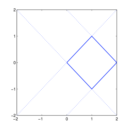
Figure 1. Solid lines are the discontinuities of the potential and dashed lines are points far from the discontinuities where the recovery fails.

4. Stability

We begin with some preliminary results that we will require for the proof of the stability estimates.

Lemma 4.1.

Let $V_{1},V_{2}\in H^{s}$, where $0<2s\leq 1$ and let $F\in L^{2}$. Then there exists a constant $C$ such that

$$\sup_{x\in\Omega}\left|T^{\lambda}_{w_{1}w_{2}}[F](x)\right|\leq C\lambda^{-2s}\left\|F\right\|_{L^{2}}\left\|V_{1}\right\|_{\dot{H}^{s}}\left\|V_{2}\right\|_{\dot{H}^{s}}$$

when $\lambda$ is sufficiently large.

Proof.

By Hölder’s inequality and the Hardy-Littlewood-Sobolev lemma we get

$$\left|T^{\lambda}_{w_{1}w_{2}}[F](x)\right| \leq \lambda\left\|Fw_{1}w_{2}\right\|_{L^{1}}$$

$$\leq \lambda\left\|F\right\|_{L^{2}}\left\|w_{1}\right\|_{L^{4}}\left\|w_{2}\right\|_{L^{4}}$$

$$\leq C\lambda\left\|F\right\|_{L^{2}}\left\|w_{1}\right\|_{\dot{H}^{1/2}}\left\|w_{2}\right\|_{\dot{H}^{1/2}}.$$

As $(I-S_{V}^{\lambda})^{-1}$ is bounded for $\lambda$ sufficiently large (see [4, Lemma 2.3]), this yields

$$\left|T^{\lambda}_{w_{1}w_{2}}[F](x)\right| \leq C\lambda\left\|F\right\|_{L^{2}}\left\|S_{1}^{\lambda}[V_{1}]\right\|_{\dot{H}^{1/2}}\left\|S_{1}^{\lambda}[V_{2}]\right\|_{\dot{H}^{1/2}}.$$

Applying Lemma 2.2 twice concludes the proof. ∎

We will also require the following crude bound for Bukhgeim solutions.

Lemma 4.2.

Let $0<r<1/2$, and let $V$ be a piecewise $W^{2,1}$-potential contained in a bounded planar domain $\Omega$ with diameter $d$. Then there exists a constant $C$ depending on $\Omega$ such that the Bukhgeim solutions satisfy

$$\left\|u_{\lambda,x}\right\|_{H^{1}(\Omega)}\leq Ce^{\lambda d^{2}}\left(1+\left\|V\right\|_{D^{2,r}}^{2}\right)$$

whenever $\lambda$ is sufficiently large.

Proof.

Writing $u=u_{\lambda,x}$,

$$\left\|u\right\|_{H^{1}(\Omega)} \leq C\left(\left\|u\right\|_{L^{2}(\Omega)}+\left\|\partial_{\overline{z}}u\right\|_{L^{2}(\Omega)}+\left\|\partial_{z}u\right\|_{L^{2}(\Omega)}\right)$$

$$= C\left\|e^{i\lambda\psi}(1+w)\right\|_{L^{2}(\Omega)}+C\left\|\partial_{z}^{-1}Ve^{i\lambda\psi}(1+w)\right\|_{L^{2}(\Omega)}$$

$$+\,C\left\|\partial_{\overline{z}}^{-1}Ve^{i\lambda\psi}(1+w)\right\|_{L^{2}(\Omega)}$$

Note that $\partial_{z}^{-1}$ and $\partial_{\overline{z}}^{-1}$ are bounded operators, as $V$ has compact support (see for example [6, Theorem 4.3.12]). As we have $\left\|\cdot\right\|_{L^{2}(\Omega)}\leq C\left\|\cdot\right\|_{L^{4}(\Omega)}$, then using Hölder’s inequality leads to

$$\left\|u\right\|_{H^{1}(\Omega)} \leq C\left\|e^{i\lambda\psi}\right\|_{L^{\infty}(\Omega)}\left(1+\left\|V\right\|_{L^{4}}\right)\left\|1+w\right\|_{L^{4}(\Omega)}$$

$$\leq Ce^{i\lambda d^{2}}\left(1+\left\|V\right\|_{L^{4}}\right)\left(1+\left\|w\right\|_{L^{4}(\Omega)}\right),$$

and by the Hardy-Littlewood-Sobolev inequality we get

$$\left\|u\right\|_{H^{1}(\Omega)} \leq Ce^{i\lambda d^{2}}\left(1+\left\|V\right\|_{L^{4}}\right)\left(1+\left\|w\right\|_{\dot{H}^{1/2}}\right).$$

As $(I-S^{\lambda}_{V})^{-1}$ is bounded for $\lambda$ sufficiently large (see [4, Lemma 2.3]), we have

$$\left\|u\right\|_{H^{1}(\Omega)}\leq Ce^{i\lambda d^{2}}\left(1+\left\|V\right\|_{L^{4}}\right)\left(1+\left\|S_{1}^{\lambda}[V]\right\|_{\dot{H}^{1/2}}\right).$$

Now, by Lemma 2.2 we get

$$\left\|u\right\|_{H^{1}(\Omega)}\leq Ce^{i\lambda d^{2}}\left(1+\left\|V\right\|_{L^{4}}\right)\left(1+\left\|V\right\|_{\dot{H}^{r}}\right).$$

Using Sobolev embedding (see for example [1, Theorem 4.12, Part 1, Case A]) we have

$$\left\|V\right\|_{L^{4}}\leq C\sum_{j=1}^{N}\left\|q_{j}\right\|_{L^{4}}\leq\left\|V\right\|_{D^{2,r}}.$$

Using part $ii)$ of Lemma 2.5 Lemma concludes the proof. ∎

We now prove an a priori stability estimate for reconstruction from the DtN map in the $L^{\infty}$ norm. Note that the result is interesting when there is a priori knowledge of where, approximately, the discontinuities lie, as the constant term depends on the point under consideration with respect to the discontinuities. The result has been stated in the following form as in practical situations one could consider where a potential might lie, given a noisy reconstruction of it. If the assumption that the discontinuities of the potentials are closed to each other was dropped, the constant $C_{x}$ would depend on both $\{\partial\Omega_{1,j}\}$ and $\{\partial\Omega_{2,j}\}$, the discontinuities of $V_{1}$ and $V_{2}$ respectively.

Theorem 4.3.

Let $0<s-2<2r<1$ and let $V_{1},V_{2}$ be piecewise $W^{s,1}$-potentials supported on a Lipschitz domain $\Omega$ in $\mathbb{R}^{2}$ such that their discontinuities are close enough with respect to the $C^{2}$ norm. Then, for almost every $x\in\Omega$, there exists a constant $C_{x}=C(x,\cup\partial\Omega_{1,j})$ such that

$$\left|V_{1}(x)-V_{2}(x)\right|\leq C_{x}\big{|}\ln\left\|\Lambda_{V_{1}}-\Lambda_{V_{2}}\right\|\big{|}^{1-s/2}(\kappa+\kappa^{3})$$

whenever $\Lambda_{V_{1}}$ and $\Lambda_{V_{2}}$ are close enough, where $\kappa=\max\{\left\|V_{1}\right\|_{D^{s,r}},\left\|V_{2}\right\|_{D^{s,r}}\}$.

Proof.

Let $d$ be the diameter of $\Omega$ and let

(19) $$\lambda=\frac{-1}{6d^{2}}\ln\left\|\Lambda_{V_{1}}-\Lambda_{V_{2}}\right\|.$$

Note that whenever $\Lambda_{V_{1}}$ and $\Lambda_{V_{2}}$ are sufficiently close, then $\lambda$ can be as large as we need.

By the triangle inequality,

$$\ \ \left|V_{1}(x)-V_{2}(x)\right| \leq \left|V_{1}(x)-T^{\lambda}_{1+w_{1}}[V_{1}](x)\right|+\left|V_{2}(x)-T^{\lambda}_{1+w_{2}}[V_{2}](x)\right|$$

$$+\left|T^{\lambda}_{1+w_{1}}[V_{1}](x)-T^{\lambda}_{1+w_{2}}[V_{2}](x)\right|.$$

We can use Theorem 3.3 on the first two terms to obtain

(21) $$\left|V_{j}(x)-T^{\lambda}_{1+w_{j}}[V_{j}](x)\right|\leq C_{x}\,\lambda^{1-s/2}(\kappa+\kappa^{2})$$

where $C_{x}=C(x,\cup\partial\Omega_{1,j})$. We can take the same constant $C_{x}$ for both terms as it is continuous with respect to the discontinuities in the $C^{2}$ norm (due to Lemma 3.6). For the last term we have

$$\left|T^{\lambda}_{1+w_{1}}[V_{1}](x)-T^{\lambda}_{1+w_{2}}[V_{2}](x)\right| \leq \left|T^{\lambda}_{(1+w_{1})(1+w_{2})}[V_{1}-V_{2}](x)\right|$$

$$+\left|T^{\lambda}_{w_{1}}[V_{2}](x)\right|+\left|T^{\lambda}_{w_{2}}[V_{1}](x)\right|$$

$$+\left|T^{\lambda}_{w_{1}w_{2}}[V_{1}-V_{2}](x)\right|.$$

By Lemma 2.3 and part $ii)$ of Lemma 2.5 we obtain

(22) $$\left\|T^{\lambda}_{w_{2}}[V_{1}]\right\|_{L^{\infty}}\leq C\,\lambda^{1-s/2}\kappa^{2}\quad\text{and}\quad\left\|T^{\lambda}_{w_{1}}[V_{2}]\right\|_{L^{\infty}}\leq C\,\lambda^{1-s/2}\kappa^{2}.$$

and by Lemma 4.1 and part $ii)$ of Lemma 2.5 we obtain

(23) $$\left\|T^{\lambda}_{w_{1}w_{2}}[V_{1}-V_{2}]\right\|_{L^{\infty}}\leq C\,\lambda^{1-s/2}\kappa^{3}.$$

Let $u_{j}$ be Bukhgeim solutions to $\Delta u_{j}=V_{j}u_{j}$. Then we have

$$\left\|T^{\lambda}_{(1+w_{1})(1+w_{2})}[V_{1}-V_{2}]\right\|_{L^{\infty}} = \frac{\lambda}{\pi}\left\|\int_{\Omega}(V_{1}-V_{2})u_{1}u_{2}\right\|_{L^{\infty}}$$

$$= \frac{\lambda}{\pi}\left\|\int_{\partial\Omega}f_{1}\Lambda_{V_{2}}[f_{2}]-f_{2}\Lambda_{V_{1}}[f_{1}]\right\|_{L^{\infty}},$$

where $f_{j}=u_{j}|_{\partial\Omega}$. As the DtN is a self-adjoint operator, we have that

$$\frac{\lambda}{\pi}\left\|\int_{\partial\Omega}f_{1}\Lambda_{V_{2}}[f_{2}]-f_{2}\Lambda_{V_{1}}[f_{1}]\right\|_{L^{\infty}}=\frac{\lambda}{\pi}\left\|\int_{\partial\Omega}\left(\Lambda_{V_{1}}-\Lambda_{V_{2}}\right)[f_{1}]f_{2}\right\|_{L^{\infty}}.$$

For $f\in H^{1/2}$ the DtN map satisfies $\Lambda_{v}[f]\in H^{-1/2}$, where $H^{-1/2}$ is the dual of $H^{1/2}$. Thus, for any $x\in\Omega$, we have

$$\frac{\lambda}{\pi}\left|\int_{\partial\Omega}\left(\Lambda_{V_{1}}-\Lambda_{V_{2}}\right)[f_{1}]f_{2}\right| \leq \lambda\left\|\Lambda_{V_{1}}-\Lambda_{V_{2}}\right\|\left\|f_{1}\right\|_{H^{1/2}(\partial\Omega)}\left\|f_{2}\right\|_{H^{1/2}(\partial\Omega)}$$

$$\leq \lambda\left\|\Lambda_{V_{1}}-\Lambda_{V_{2}}\right\|\left\|u_{1}\right\|_{H^{1}(\Omega)}\left\|u_{2}\right\|_{H^{1}(\Omega)}$$

and we can use Lemma 4.2 to obtain

(24) $$\frac{\lambda}{\pi}\left|\int_{\partial\Omega}\left(\Lambda_{V_{1}}-\Lambda_{V_{2}}\right)[f_{1}]f_{2}\right|\leq C\lambda e^{2\lambda d^{2}}\left\|\Lambda_{V_{1}}-\Lambda_{V_{2}}\right\|\left(1+\kappa^{4}\right).$$

Inserting (21), (22), (23) and (24) into (4), and noting that $\lambda<e^{\lambda d}$ for $\lambda$ sufficiently large, leads to

$$\left|V_{1}(x)-V_{2}(x)\right|\leq C_{x}\ \lambda^{1-s/2}\ (\kappa+\kappa^{3})+\,C\left\|\Lambda_{V_{1}}-\Lambda_{V_{2}}\right\|e^{3\lambda d^{2}}(1+\kappa^{4}).$$

Taking $\lambda$ as in (19) we obtain

$$\left|V_{1}(x)-V_{2}(x)\right| \leq C_{x}\left(\frac{-1}{6d^{2}}\ln\left\|\Lambda_{V_{1}}-\Lambda_{V_{2}}\right\|\right)^{1-s/2}(1+\kappa^{3})$$

$$+\,C\left\|\Lambda_{V_{1}}-\Lambda_{V_{2}}\right\|^{1/2}(1+\kappa^{4})$$

where the second term can be omitted for $\left\|\Lambda_{V_{1}}-\Lambda_{V_{2}}\right\|$ small enough, concluding the proof. ∎

We now provide a link to the scattering amplitude. We adapt the proof of Stefanov (see [33]) to the two-dimensional case. Due to the severe ill-posedness of the problem, we need to introduce a norm for the scattering amplitude which penalizes the higher components of the frequency spectrum. Let $V$ be a potential supported on the unit disk, then we define the norm for its scattering amplitude at a fixed energy $k^{2}$ as

$$\left\|A_{V}\right\|_{k}=\left(\sum_{n,m\in\mathbb{Z}}\left(\frac{3+3\left|n\right|}{k}\right)^{2\left|n\right|}\left(\frac{3+3\left|m\right|}{k}\right)^{2\left|m\right|}\left|a^{(n,m)}_{V}\right|^{2}\right)^{1/2},$$

where $a^{(n,m)}_{V}$ are the Fourier coefficients of $A_{V}$

$$A_{V}(\eta,\theta)=\sum_{n,m\in\mathbb{Z}}a^{(n,m)}_{V}e^{in\eta+im\theta}.$$

Before passing to the proof, we define the single layer potential operator

$$\mathcal{S}_{V}[f](x)=\int_{\partial\Omega}G_{V}(x,y)f(y)dy,$$

where $G_{V}$ is the outgoing Green’s function which satisfies

$$(-\Delta+V-k^{2})\,G_{V}(x,y)=\delta(x-y).$$

Lemma 4.4.

Let $V_{1},V_{2}$ be two potentials supported in the unit disk. Then there exists a constant $C_{k}=C(k)$ such that

$$\left\|\Lambda_{V_{1}}-\Lambda_{V_{2}}\right\|_{H^{1/2}(\mathbb{S}^{1})\rightarrow H^{-1/2}(\mathbb{S}^{1})}\leq C_{k}\left\|A_{V_{1}}-A_{V_{2}}\right\|_{k}.$$

Proof.

Using Nachman’s formula [27, Theorem 1.6] we have

$$\Lambda_{V_{1}-k^{2}}-\Lambda_{V_{2}-k^{2}} = \mathcal{S}_{V_{1}}^{-1}-\mathcal{S}_{V_{2}}^{-1}$$

$$= \mathcal{S}_{V_{1}}^{-1}\left(\mathcal{S}_{V_{2}}-\mathcal{S}_{V_{1}}\right)\mathcal{S}_{V_{2}}^{-1}.$$

As $\mathcal{S}_{V}$ is a bounded and invertible mapping from $H^{-1/2}(\mathbb{S}^{1})$ to $H^{1/2}(\mathbb{S}^{1})$ (see [23, Proposition A.1]), we have

$$\left\|\Lambda_{V_{1}-k^{2}}-\Lambda_{V_{2}-k^{2}}\right\|_{H^{1/2}(\mathbb{S}^{1})\rightarrow H^{-1/2}(\mathbb{S}^{1})}\leq C\left\|\mathcal{S}_{V_{1}}-\mathcal{S}_{V_{2}}\right\|_{H^{-1/2}(\mathbb{S}^{1})\rightarrow H^{1/2}(\mathbb{S}^{1})}.$$

Letting $B_{x}=(1-\Delta_{x})^{1/4}$, we write

$$\left\|\mathcal{S}_{V_{1}}-\mathcal{S}_{V_{2}}\right\|_{H^{-1/2}(\mathbb{S}^{1})\rightarrow H^{1/2}(\mathbb{S}^{1})}$$

$$=\sup_{\left\|f\right\|=1}\left\|\int_{\mathbb{S}^{1}}(G_{V_{1}}(x,y)-G_{V_{2}}(x,y))f(y)\,dy\right\|_{H^{1/2}(\mathbb{S}^{1})}$$

$$=\sup_{\left\|f\right\|=1}\left(\int_{\mathbb{S}^{1}}\left(B_{x}\int_{\mathbb{S}^{1}}(G_{V_{1}}(x,y)-G_{V_{2}}(x,y))f(y)\,dy\right)^{2}dx\right)^{1/2}$$

$$=\sup_{\left\|f\right\|=1}\left(\int_{\mathbb{S}^{1}}\left(\int_{\mathbb{S}^{1}}B_{x}(G_{V_{1}}(x,y)-G_{V_{2}}(x,y))f(y)\,dy\right)^{2}dx\right)^{1/2}$$

by Pareseval’s identity we have

$$=\sup_{\left\|f\right\|=1}\left(\int_{\mathbb{S}^{1}}\left(\int_{\mathbb{S}^{1}}\left(B_{y}B_{x}(G_{V_{1}}(x,y)-G_{V_{2}}(x,y))\right)B_{y}^{-1}f(y)dy\right)^{2}dx\right)^{1/2}$$

using Minkowski’s integral inequality we get

$$\leq\sup_{\left\|f\right\|=1}\int_{\mathbb{S}^{1}}\left(\int_{\mathbb{S}^{1}}\left(\left(B_{y}B_{x}(G_{V_{1}}(x,y)-G_{V_{2}}(x,y))\right)B_{y}^{-1}f(y)\right)^{2}dx\right)^{1/2}dy$$

$$=\sup_{\left\|f\right\|=1}\int_{\mathbb{S}^{1}}\left|B_{y}^{-1}f(y)\right|\left(\int_{\mathbb{S}^{1}}\left(B_{y}B_{x}(G_{V_{1}}(x,y)-G_{V_{2}}(x,y))\right)^{2}dx\right)^{1/2}dy$$

and using the Cauchy-Schwarz inequality

$$\leq\sup_{\left\|f\right\|=1}\left\|f\right\|_{H^{-1/2}(\mathbb{S}^{1})}\left\|G_{V_{1}}-G_{V_{2}}\right\|_{H^{1/2}(\mathbb{S}^{1})\otimes H^{1/2}(\mathbb{S}^{1})}$$

$$=\left\|G_{V_{1}}-G_{V_{2}}\right\|_{H^{1/2}(\mathbb{S}^{1})\otimes H^{1/2}(\mathbb{S}^{1})}.$$

From [5, Theorem 2.2] we know that

$$G_{V_{1}}(x,y)-G_{V_{2}}(x,y) = \sum_{n,m\in\mathbb{Z}}\frac{(-1)^{n}}{16}i^{n+m}\left(a^{(n,m)}_{V_{1}}-a^{(n,m)}_{V_{2}}\right)$$

$$\times\,H^{(1)}_{n}(k\left|x\right|)\,H^{(1)}_{m}(k\left|y\right|)\,e^{in\phi_{x}+im\phi_{y}}$$

where $H^{(1)}$ denotes the Hankel function of the first kind. Now, using Parseval’s identity and the bound for the Hankel function in [5, Lemma 2.3], there exists $C_{k}^{\prime}=C(k)$ such that

$$\left\|G_{V_{1}}-G_{V_{2}}\right\|_{H^{1/2}(\mathbb{S}^{1})\otimes H^{1/2}(\mathbb{S}^{1})}^{2}$$

$$\leq \sum_{n,m\in\mathbb{Z}}(1+n^{2})^{1/2}(1+m^{2})^{1/2}\left|a^{(n,m)}_{V_{1}}-a^{(n,m)}_{V_{2}}\right|^{2}\left|H^{(1)}_{n}(k)\right|^{2}\left|H^{(1)}_{m}(k)\right|^{2}$$

$$\leq C_{k}^{\prime}\sum_{n,m\in\mathbb{Z}}(1+n^{2})^{1/2}(1+m^{2})^{1/2}\left|a^{(n,m)}_{V_{1}}-a^{(n,m)}_{V_{2}}\right|^{2}{\left|n\right|!}^{2}{\left|m\right|!}^{2}\left(\frac{3}{k}\right)^{2\left|n\right|+2\left|m\right|}$$

$$\leq C_{k}^{\prime}\sum_{n,m\in\mathbb{Z}}\left(\frac{3+3\left|n\right|}{k}\right)^{2\left|n\right|}\left(\frac{3+3\left|m\right|}{k}\right)^{2\left|m\right|}\left|a^{(n,m)}_{V_{1}}-a^{(n,m)}_{V_{2}}\right|^{2}$$

concluding the proof. ∎

Corollary 4.5.

Let $0<s-2<2r<1$ and let $V_{1},V_{2}$ be two piecewise $W^{s,1}$ potentials supported on a bounded domain in $\mathbb{R}^{2}$ such that their discontinuities are close enough in the $C^{2}$ norm. Then, for almost every $x\in\Omega$, there exist constants $C_{x}=C(x,\cup\partial\Omega_{j}),C_{k}=C(k),$ such that

$$\left|V_{1}(x)-V_{2}(x)\right|\leq C_{x}\big{|}\ln\left(C_{k}\left\|A_{V_{1}}-A_{V_{2}}\right\|_{k}\right)\big{|}^{1-s/2}(\kappa+\kappa^{3})$$

whenever $\Lambda_{V_{1}}$ and $\Lambda_{V_{2}}$ are close enough, where $\kappa=\max\{\left\|V_{1}\right\|_{D^{s,r}},\left\|V_{2}\right\|_{D^{s,r}}\}$.

Acknowledgements: The author thanks Daniel Faraco and Keith Rogers for their valuable comments and corrections and thanks Evgeny Lakshtanov for bringing [26] to his attention. This work has been partially supported by ERC-277778 and by ICMAT Severo Ochoa project SEV-2015-0554 (MINECO).

References

- [1] R. A. Adams and John J. F. Fournier. Sobolev Spaces. Pure and Applied Mathematics, Elsevier (2003).
- [2] G. Alessandrini. Stable determination of conductivity by boundary measurements. Applicable Analysis (1988).
- [3] G. Alessandrini. Global stability for a coupled physics inverse problem. Inverse Problems (2014).
- [4] K. Astala, D. Faraco and K. M. Rogers. Unbounded potential recovery in the plane. Annales scientifiques de l’École Normale Supérieure, to appear, arXiv:1304.1317 (2015).
- [5] K. Astala, D. Faraco and K. M. Rogers. Recovery of the Dirichlet-to-Neumann map from scattering data in the plane. RIMS Kokyuroku Bessatsu (2014).
- [6] K. Astala, T. Iwaniec and G. Martin. Elliptic Partial Differential Equations and Quasiconformal Mappings in the Plane. Princeton University Press (2008).
- [7] K. Astala and L. Päivärinta. Calderón Inverse Conductivity problem in plane. Annals of Mathematics (2006).
- [8] J. A. Barceló, T. Barceló and A. Ruiz. Stability of the Inverse Conductivity Problem in the Plane for Less Regular Conductivities. Journal of Differential Equations (2001).
- [9] T. Barceló , D. Faraco and A. Ruiz. Stability of Calderón inverse conductivity problem in the plane. Journal de Mathématiques Pures et Appliquées (2007).
- [10] E. Blasten, O. Yu. Imanuvilov and M. Yamamoto. Stability and uniqueness for a two-dimensional inverse boundary value problem for less regular potentials. Inverse Problems and Imaging (2015).
- [11] R. M. Brown and R. H. Torres. Uniqueness in the inverse conductivity problem for conductivities with 3/2 derivatives in . Journal of Fourier Analysis and Applications (2003).
- [12] R. M. Brown and G. A. Uhlmann. Uniqueness in the inverse conductivity problem for nonsmooth conductivities in two dimensions. Communications in Partial Differential Equations (1997).
- [13] A. L. Bukhgeim. Recovering a potential from Cauchy data in the two-dimensional case. Journal of Inverse and Ill-Posed Problems (2008).
- [14] A. P. Calderón. On an inverse boundary value problem. Seminar on Numerical Analysis and its Applications to Continuum Physics, Rio de Janeiro (1980).
- [15] P. Caro, A. García and J. M. Reyes. Stability of the Calderón problem for less regular conductivities. Journal of Differential Equations (2013).
- [16] P. Caro and K. M. Rogers. Global uniqueness for the Calderón problem with Lipschitz conductivities. Forum of Mathematics Pi (2016).
- [17] A. Clop, D. Faraco and A. Ruiz. Stability of Calderón’s inverse conductivity problem in the plane for discontinuous conductivities. Inverse Problems and Imaging (2010).
- [18] L. C. Evans. Partial Differential Equations. Graduate Studies in Mathematics (2010).
- [19] D. Faraco and K. M. Rogers. The Sobolev norm of characteristic functions with applications to the Calderón inverse problem. The Quarterly Journal of Mathematics (2013).
- [20] L. Grafakos. Classical Fourier analysis. Springer, Graduate Texts in Mathematics (2008).
- [21] B. Haberman. Uniqueness in Calderón’s problem for conductivities with unbounded gradient. Communications on Mathematical Physics (2015).
- [22] B. Haberman, D. Tataru. Uniqueness in Calderón’s problem with Lipschitz conductivities. Duke Mathematical Journal (2013).
- [23] V. Isakov and A. I. Nachman. Global uniqueness for a two-dimensional semilinear elliptic inverse problem. Transactions of the American Mathematical Society (1995).
- [24] C. Kenig, G. Ponce and L. Vega. Well-posedness and scattering results for the generalized Korteweg-de Vries equation via the contraction principle. Communications in Pure and Applied Mathematics (1993).
- [25] C. Kenig, J. Sjöstrand and G. Uhlmann. The Calderón problem with partial data. Annals of Mathematics (2007).
- [26] E. L. Lakshtanov, R. G. Novikov and B. R. Vainberg. A global Riemann-Hilbert problem for two-dimensional inverse scattering at fixed energy. arXiv:1509.06495 (2015).
- [27] A. I. Nachman. Reconstructions from boundary measurements. Annals of Mathematics (1988).
- [28] A. I. Nachman. Global uniqueness for a two-dimensional inverse boundary value problem. Annals of Mathematics (1996).
- [29] R. G. Novikov. Multidimensional inverse spectral problem for the equation . Functional Analysis and Its Applications (1988).
- [30] R. G. Novikov and M. Santacesaria. A global stability estimate for the Gel’fand-Calderón inverse problem in two dimensions. Journal of Inverse and Ill-Posed Problems (2010).
- [31] R. G. Novikov and M. Santacesaria. Global uniqueness and reconstruction for the multi-channel Gel’fand-Calderón inverse problem in two dimensions. Bulletin des Sciences Mathématiques (2011).
- [32] K. M. Rogers, A. Vargas and L. Vega. Pointwise convergence of solutions to the nonelliptic Schrödinger equation. Indiana University Mathematical Journal (2006).
- [33] P. Stefanov. Stability of the inverse problem in potential scattering at fixed energy. Annales de l’institue Fourier (1990).
- [34] J. Sylvester and G. Uhlmann. A global uniqueness theorem for an inverse boundary value problem. Annals of Mathematics (1987).