AdS/QCD approach to the scale-invariant extension of the standard model with a strongly interacting hidden sector

Abstract

In this paper, we revisit a scale-invariant extension of the standard model (SM) with a strongly interacting hidden sector within AdS/QCD approach. Using the AdS/QCD, we reduce the number of input parameters to three, i.e. hidden pion decay constant, hidden pion mass and $\tan\beta$ that is defined as the ratio of the vacuum expectation values (VEV) of the singlet scalar field and the SM Higgs boson. As a result, our model has sharp predictability. We perform the phenomenological analysis of the hidden pions which is one of the dark matter (DM) candidates in this model. With various theoretical and experimental constraints we search for the allowed parameter space and find that both resonance and non-resonance solutions are possible. Some typical correlations among various observables such as thermal relic density of hidden pions, Higgs boson signal strengths and DM-nucleon cross section are investigated. We provide some benchmark points for experimental tests.

I Introduction

Although the SM-like Higgs boson has been discovered at the Large Hadron Collider (LHC) Aad:2012tfa ; Chatrchyan:2012xdj , there are still a number of questions that call for physics beyond the SM (BSM): (i) the origin of the mass of Higgs particle or the origin of weak scale, (ii) the nature of non-baryonic dark matter (DM), (iii) the origin of neutrino masses and mixing, (iv) matter-antimatter asymmetry of the universe, to name a few.

The first question is often phrased as hierarchy problem, that addresses why the electroweak (EW) scale $v_{H}=246$ GeV is much smaller than the Planck scale. One of the nice ways to understand this is through quantum dimensional transmutation, which explains why the proton mass is much suppressed compared with the Planck mass in Quantum Chromodynamics (QCD) Hill:2002ap ; Wilczek:2005ez . Technicolor (TC) provides an answer in this way, but the naive version of it is strongly disfavored by the electroweak precision test (EWPT) Peskin:1990zt .

Since the observation of W. Bardeen Bardeen:1995kv , softly broken scale invariance has been considered as a possible solution for the hierarchy problem. If the model is scale invariant at classical level, no dimensionful parameters are allowed and the scale symmetry is broken only logarithmically through scale-anomaly. Many authors have studies this type of models where the EW symmetry is dynamically broken via dimensional transmutation in the hidden sector with new confining strong interactions Hur:2007uz ; Ko:2008ug ; Ko:2009zz ; Ko:2010rj ; Hur:2011sv ; Heikinheimo:2013fta ; Heikinheimo:2013xua ; Holthausen:2013ota ; Jung:2014zga ; Salvio:2014soa ; Kubo:2014ova ; Kubo:2014ida ; Schwaller:2015tja ; Ametani:2015jla ; Kubo:2015joa ; Haba:2015qbz , or Coleman-Weinberg mechanism Meissner:2006zh ; Foot:2007as ; Meissner:2007xv ; Hambye:2007vf ; Foot:2007iy ; Iso:2009ss ; Iso:2009nw ; Holthausen:2009uc ; AlexanderNunneley:2010nw ; Ishiwata:2011aa ; Lee:2012jn ; Okada:2012sg ; Iso:2012jn ; Gherghetta:2012gb ; Das:2011wm ; Carone:2013wla ; Khoze:2013oga ; Farzinnia:2013pga ; Antipin:2013exa ; Hashimoto:2014ela ; Hill:2014mqa ; Guo:2014bha ; Radovcic:2014rea ; Binjonaid:2014oga ; Allison:2014zya ; Farzinnia:2014xia ; Pelaggi:2014wba ; Farzinnia:2014yqa ; Foot:2014ifa ; Benic:2014aga ; Guo:2015lxa ; Oda:2015gna ; Fuyuto:2015vna ; Endo:2015nba ; Plascencia:2015xwa ; Hashino:2015nxa ; Karam:2015jta ; Ahriche:2015loa ; Wang:2015cda ; Haba:2015nwl ; Ghorbani:2015xvz ; Helmboldt:2016mpi ; Jinno:2016knw ; Ahriche:2016cio ; Ahriche:2016ixu ; Das:2016zue ; Khoze:2016zfi .

Some of the present authors have proposed a scale-invariant extensions of the SM with a strongly interacting hidden sector, namely hidden QCD models Hur:2007uz ; Ko:2008ug ; Ko:2009zz ; Ko:2010rj ; Hur:2011sv ; Hur:2011sv . At the classical level, the scale invariance is imposed so that all dimensionful parameters are forbidden in the classical Lagrangian. The Higgs mass term arises at quantum level through the dimensional transmutation driven by asymptotically free gauge theories in the hidden sector. Hidden sector couples to the Higgs through singlet scalar field only and there are stable or long-lived particles (lightest hidden mesons and hidden baryons) that can make good DM candidates. In those works, hidden QCD sector was studied in the chiral effective Lagrangian approach and non-perturbative parameters were estimated by naive dimensional analysis. Then the same model was analyzed in the Nambu–Jona-Lasinio (NJL) approach in Ref. Holthausen:2013ota ; Kubo:2014ida .

In this paper, we consider the same model using another approximation method, the AdS/QCD DaRold:2005zs ; DaRold:2005vr , in order to analyze non-perturbative strong dynamics in the hidden QCD models. First we reformulate the hidden QCD sector in terms of the linear sigma model, in which the sigma and pi mesons are effective degrees of freedom. We consider a linear sigma model coupled with a scale-invariant Higgs-singlet sector and analyzed the masses and mixing between the SM Higgs boson, a singlet scalar messenger and the sigma meson. In the AdS/QCD we successfully reduce the number of free parameters by matching the mass spectra of the lightest scalar, vector and axial vector mesons.

Next, we apply this model to dark matter phenomenology. In our model, since the hidden quarks do not couple to any U(1) gauge fields, the hidden pions cannot decay through the U(1) anomaly and are found to be stable lightest particles coupling weakly with the SM fields. Hence the hidden pions become candidates of the weakly interacting massive particle (WIMP) DM. With the free parameters reduced by the AdS/QCD, we identify the parameter space that satisfies the recent observations. Then we study the distinctive features of the allowed parameter region and also some typical correlations among various observables. We address on the possible signatures of the model that can be further scrutinized in the future experiments such as LHC Run-II, ILC and so forth.

This paper is organized as follows. In Sec. II, we revisit the original hidden QCD models Hur:2007uz ; Hur:2011sv by reformulating the hidden QCD sector with the linear sigma model. Then in Sec. III, we apply the idea of the AdS/QCD to the linear sigma model described in Sec. II. In Sec. IV, numerical results on the Higgs and the dark matter phenomenologies are presented. Then Sec. V is devoted to summary and discussions.

II The Model

Scale-invariant extension of the SM with a strongly interacting hidden sector contains the SM fields plus a singlet scalar $S$ and a scale-invariant hidden QCD sector Ko:2008ug ; Ko:2009zz ; Ko:2010rj ; Hur:2011sv . The corresponding Lagrangian is given by

$${\cal L} = {\cal L}_{\rm SM}(\mu_{H}^{2}=0)+\frac{1}{2}(\partial_{\mu}S)^{2}-\frac{\lambda_{S}}{8}S^{4}+\frac{\lambda_{HS}}{2}H^{\dagger}HS^{2}-\frac{1}{2}Y^{ij}_{N_{R}}S\overline{N_{Ri}^{c}}N_{Rj}$$ (1)

$$-\left(Y_{N}^{ij}\overline{N_{Ri}}\widetilde{H}l_{Lj}+H.c.\right)-\frac{1}{2}\text{tr}\,{G}_{\mu\nu}G^{\mu\nu}+\sum_{k=1}^{N_{h,f}}\overline{Q_{k}}(i\gamma^{\mu}D_{\mu}-\lambda_{Q,k}S)Q_{k},$$

where $\mu_{H}$ is the mass parameter of the SM Higgs boson. We have replaced all the mass parameters (the Higgs boson mass, the RH neutrino masses and the current quark masses of hidden-sector quarks) by real singlet scalar operators $S$ or $S^{2}$ following the idea of classical scale invariance. $G_{\mu\nu}$ is the field strength of the hidden QCD with $SU(N_{h,c})$ gauge symmetry. The SM singlet scalar $S$ couples to the hidden-sector quarks $Q_{f}$ through the Yukawa interaction. Since there are no dimensionful parameters in the Lagrangian, this system is scale-invariant at the classical level. At quantum level and low-energy scale, the hidden-QCD quarks can condensate. Such condensates $\langle\bar{Q}Q\rangle$ induce a linear term in $S$. Then the potential of $S$ can be tilted and $S$ can develop a VEV. The VEV of the singlet scalar generates a Higgs boson mass term $-\frac{\lambda_{HS}}{2}\langle S\rangle^{2}H^{\dagger}H$, as well as the RH neutrino masses and the current quark masses of the hidden-sector quarks. Thus all the mass scales in this model are generated by $\langle S\rangle$, which is a result of non-perturbative dynamics in the strongly interacting hidden sector. For this to happen, we assume that $\lambda_{HS}>0$ so that non-zero $\langle S\rangle$ triggers the electroweak symmetry breaking.

Hereafter we consider the case in which $N_{h,c}=3$ and $N_{h,f}=2$, for which we can use the known results from the hadronic system with $\pi,\rho$ and $\sigma$ mesons. Then $\lambda_{Q}=\text{diag}(\lambda_{Qu},\lambda_{Qd})$ and for simplicity we assume the hidden quarks have isospin symmetry $\lambda_{Qu}\sim\lambda_{Qd}$. In such a case the low-energy effective theory of the hidden QCD is described by the pi meson triplets and the sigma meson. It would be written in the form of a linear sigma model

$${\cal L}_{L\sigma M} = \frac{1}{2}(\partial_{\mu}\Sigma)^{2}+\frac{1}{2}(\partial_{\mu}\pi)^{2}+\frac{\lambda_{\sigma}}{4}(\Sigma^{2}+\pi^{2})^{2}-\frac{\mu_{\sigma}^{2}}{2}(\Sigma^{2}+\pi^{2})-m_{S\sigma}^{2}S\Sigma,$$ (2)

where $\Sigma$ and $\pi$ represents sigma and pi meson fields.

We parameterize the VEVs and fluctuations of scalars as

$$H=\frac{1}{\sqrt{2}}\begin{pmatrix}0\\ v_{H}+h\end{pmatrix},\quad S=v_{S}+s,\quad\Sigma=v_{\sigma}+\sigma.$$ (3)

To minimize the potential energy

$$V(v_{H},v_{S},v_{\sigma}) = \frac{\lambda_{H}}{8}v_{H}^{4}-\frac{\lambda_{HS}}{4}v_{H}^{2}v_{S}^{2}+\frac{\lambda_{S}}{8}v_{S}^{4}+\frac{\lambda_{\sigma}}{4}v_{\sigma}^{4}-\frac{\mu_{\sigma}^{2}}{2}v_{\sigma}^{2}-m_{S\sigma}^{2}v_{S}v_{\sigma},$$ (4)

three minimization conditions $\partial V/\partial v_{\phi}=0$ ($\phi=H,S,\sigma$) should be satisfied. These conditions reduce the number of free parameters. Furthermore, two parameters $\lambda_{\sigma}$, $\mu_{\sigma}$ are traded with the pion mass $M_{\pi}$ and a sigma meson mass parameter $M_{\sigma\sigma}$. Hence the scalar mass matrix ${\cal L}\supset-\frac{1}{2}(h,s,\sigma){\cal M}(h,s,\sigma)^{T}$ takes the form of

$${\cal M} = \begin{pmatrix}M_{hh}^{2}&M_{hs}^{2}&0\\ M_{hs}^{2}&M_{ss}^{2}&-m_{S\sigma}^{2}\\ 0&-m_{S\sigma}^{2}&M_{\sigma\sigma}^{2}\end{pmatrix}$$ (5)

with

$$M_{hh}^{2} = \lambda_{H}v_{H}^{2}=\lambda_{HS}v_{H}^{2}\tan^{2}\beta,$$ (6)

$$M_{hs}^{2} = -\lambda_{HS}v_{H}^{2}\tan\beta,$$ (7)

$$M_{ss}^{2} = \lambda_{HS}v_{H}^{2}\left(1+\frac{3M_{\pi}^{2}F_{\pi}^{2}}{\lambda_{HS}\tan^{2}\beta v_{H}^{4}}\right),$$ (8)

$$-m_{S\sigma}^{2} = -\frac{M_{\pi}^{2}F_{\pi}}{v_{S}},$$ (9)

where $\tan\beta\equiv v_{S}/v_{H}$ and $F_{\pi}\equiv v_{\sigma}$. Since a off-diagonal part $M_{hs}^{2}$ satisfies $M_{hs}^{2}=-M_{hh}^{2}/\tan\beta$, the Higgs-singlet mixing can be large when $\tan\beta$ is small. $\lambda_{\sigma}$ and $\mu_{\sigma}$ are traded with pion mass $M_{\pi}$ and sigma meson mass $M_{\sigma\sigma}$ by

$$\lambda_{\sigma}=\frac{M_{\sigma\sigma}^{2}-M_{\pi}^{2}}{2F_{\pi}^{2}},\quad\mu_{\sigma}^{2}=\frac{M_{\sigma\sigma}^{2}-3M_{\pi}^{2}}{2}.$$ (10)

The couplings $\lambda_{H}$, $\lambda_{S}$ are given by

$$\lambda_{H}=\lambda_{HS}\tan^{2}\beta,\quad\lambda_{S}=\frac{\lambda_{HS}v_{H}^{4}\tan^{2}\beta+2M_{\pi}^{2}F_{\pi}^{2}}{v_{H}^{4}\tan^{4}\beta},$$ (11)

where $v_{H}=246~{}\text{GeV}$. Since one of the physical scalar should be the Higgs boson with mass $M_{H}=125~{}\text{GeV}$, $M_{H}^{2}$ is one of the eigenvalues of ${\cal M}$. Thus a condition $\det({\cal M}-M_{H}^{2}I_{3})=0$ ($I_{3}$ is a $3\times 3$ unit matrix) yields

$$\lambda_{HS} = \frac{1}{v_{S}^{2}}\frac{3\xi_{\sigma}^{2}F_{\pi}^{4}M_{\pi}^{2}-F_{\pi}^{2}M_{H}^{2}[3M_{H}^{2}M_{\pi}^{2}+M_{\pi}^{4}+M_{H}^{2}\xi_{\sigma}^{2}v_{H}^{2}\tan^{2}\beta]+M_{H}^{6}v_{H}^{2}\tan^{2}\beta}{3\xi_{\sigma}^{2}F_{\pi}^{4}-F_{\pi}^{2}[3M_{\pi}^{2}M_{H}^{2}+M_{\pi}^{4}+M_{H}^{2}v_{H}^{2}(1+\tan^{2}\beta)\xi_{\sigma}^{2}]+M_{H}^{4}v_{H}^{2}(1+\tan^{2}\beta)},$$ (12)

where we have parameterized $M_{\sigma\sigma}=\xi_{\sigma}F_{\pi}$.

The mixing matrix is defined as

$$\left(\begin{array}[]{c}h\\ s\\ \tilde{\sigma}\end{array}\right)=\left(\begin{array}[]{ccc}V_{h0}&V_{h1}&V_{h2}\\ V_{s0}&V_{s1}&V_{s2}\\ V_{\sigma 0}&V_{\sigma 1}&V_{\sigma 2}\\ \end{array}\right)\left(\begin{array}[]{c}H\\ H_{1}\\ H_{2}\end{array}\right),$$ (13)

where $H$ is the SM-like Higgs boson with $M_{H}=125$ GeV and $H_{1},H_{2}$ are extra scalar particles with $M_{H1}<M_{H2}$.

At this stage we have four free parameters: $v_{S}$, $v_{\sigma}\equiv F_{\pi}$, $M_{\pi}$ and $M_{\sigma\sigma}$ (or $\xi_{\sigma}$). To reduce the number of free parameters, in particular, to relate the $M_{\sigma\sigma}$ with $F_{\pi}$, we use a holographic treatment of the hidden QCD.

III AdS/QCD analysis

In the AdS/QCD DaRold:2005zs ; DaRold:2005vr , the hidden QCD sector is described by $SU(2)_{L}\otimes SU(2)_{R}$ gauge theory on $AdS_{5}$ space with metric

$$ds^{2} = a^{2}(z)(\eta_{\mu\nu}dx^{\mu}dx^{\nu}-dz^{2}),\quad a(z)=\frac{L}{z},$$ (14)

where $L_{0}\leq z\leq L_{1}$ and $L$ is the curvature radius of $AdS_{5}$. $L_{1}$ breaks the conformal symmetry in the infrared (IR) regime, while one can take $L_{0}$ to be arbitrary small, $L_{0}\to 0$. The non-perturbative breaking of chiral symmetry is regarded as the spontaneous breaking of $SU(2)_{L}\otimes SU(2)_{R}$ symmetry by the VEV of the bulk scalar $\Phi$ which is a bi-doublet $(\bm{2}_{L},\bm{\bar{2}}_{R})$. The parity transformation corresponds to the exchange $SU(2)_{L}\leftrightarrow SU(2)_{R}$.

Then the 5D bulk Lagrangian is given by

$$S_{5} = \int d^{4}x\int_{L_{0}}^{L_{1}}dy\sqrt{g}M_{5}\text{Tr}\left[-\frac{1}{4}L_{MN}L^{MN}-\frac{1}{4}R_{MN}R^{MN}+\frac{1}{2}|D_{M}\Phi|^{2}-\frac{1}{2}M_{\Phi}^{2}|\Phi|^{2}\right],$$ (15)

where $D_{M}\Phi=\partial_{M}\Phi+iL_{M}\Phi-i\Phi R_{M}$, $M=(\mu,5)$, and the bulk mass parameter $M_{\Phi}^{2}=-3/L^{2}$ is chosen so as to relate the bulk scalar field $\Phi$ with the dimension-three operator $\bar{q}q$. The profile of the VEV is obtained by solving the zero-mode equation of motion. We have

$$\langle\Phi\rangle\equiv v(z)=c_{1}z+c_{2}z^{3},\quad v\propto 1_{2\times 2},$$ (16)

where $c_{1}$ and $c_{2}$ can be written in terms of the value of $v$ at boundaries

$$c_{1}=\frac{\tilde{M}_{q}L_{1}^{3}-\xi L_{0}^{3}}{LL_{1}(L_{1}^{2}-L_{0}^{2})},\quad c_{2}=\frac{\xi-\tilde{M}_{q}L_{1}}{LL_{1}(L_{1}^{2}-L_{0}^{2})},$$ (17)

from boundary conditions

$$\tilde{M}_{q}=\frac{L}{L_{0}}v|_{L_{0}},\quad\xi=Lv|_{L_{1}}.$$ (18)

Here nonzero $c_{2}$ corresponds to the spontaneous breaking of the chiral symmetry in the IR, while the boundary condition at $z=L_{0}$ corresponds to the explicit breaking of chiral symmetry. The boundary condition at $z=L_{1}$ is induced by the scalar potential localized on $z=L_{1}$ boundary. The boundary interaction is

$${\cal L}_{IR} = -a^{4}V(\Phi)|_{L_{1}},\quad V(\Phi)=-\frac{1}{2}m_{b}^{2}\text{Tr}|\Phi|^{2}+\lambda_{b}\text{Tr}|\Phi|^{4}.$$ (19)

After the symmetry breaking $SU(2)_{L}\times SU(2)_{R}\to SU(2)_{V}$, vector- and axial-vector gauge bosons $V_{\mu}=(L_{\mu}+R_{\mu})/\sqrt{2}$, $A_{\mu}=(L_{\mu}-R_{\mu})/\sqrt{2}$ are expanded into Kaluza-Klein (KK) modes

$$V_{\mu}=\frac{1}{\sqrt{M_{5}L}}\sum_{n=0}^{\infty}f_{n}^{V}(z)V^{(n)}(x),\quad A_{\mu}=\frac{1}{\sqrt{M_{5}L}}\sum_{n=1}^{\infty}f_{n}^{A}(z)A^{(n)}(x),$$ (20)

where $V^{(n)}$, $A^{(n)}$ correspond to hadronic vector and axial-vector currents, respectively.

The bulk scalar $\Phi$ is decomposed into $\Phi=(v+\Phi_{S})e^{i\Phi_{P}/v}$ and gauge fixing conditions are

$$\partial_{5}(aV_{5})=0,\quad\Phi_{P}=-\frac{1}{\sqrt{2}a^{3}v}\partial_{5}(aA_{5}),$$ (21)

and $\Phi_{P,S}(x,z)$ have the following KK expansions:

$$\Phi_{S}(x,z)=\frac{1}{\sqrt{M_{5}L}}\sum_{n=1}^{\infty}f_{n}^{S}(z)S^{(n)}(x),\quad\Phi_{P}(x,z)=\frac{1}{\sqrt{M_{5}L}}\sum_{n=0}^{\infty}f_{n}^{P}(z)P^{(n)}(x),$$ (22)

where $S^{(n)}$ and $P^{(n)}$ are scalar and pseudo-scalar hadronic states, respectively. In particular $P^{(0)}$ corresponds to the pion.

In the QCD the two point correlators for the scalars and pseudoscalars are defined as

$$\Pi_{S,P}(p^{2})=-\int d^{4}xe^{ipx}\langle J_{S,P}(x)J_{S,P}(0)\rangle,\quad J_{S}=\bar{q}q,\quad J_{P}=\bar{q}i\gamma_{5}q,$$ (23)

where the two-point correlator can be obtained from the generating function ${\cal S}$ according to

$$\Pi_{S}=\frac{\delta^{2}{\cal S}}{\delta\hat{s}^{2}},\quad\Pi_{P}=\frac{\delta^{2}{\cal S}}{\delta\hat{p}_{s}^{2}},$$ (24)

where $\hat{s}$ and $\hat{p}_{s}$ are the scalar and pseudoscalar external sources coupled to QCD:

$${\cal L}\supset-\text{Tr}[\bar{q}_{L}\phi q_{R}]+h.c.,\quad\phi=M_{q}+\hat{s}+i\hat{p}_{s}.$$ (25)

According to the AdS/CFT correspondence, the generating function ${\cal S}$ is obtained by integrating bulk fields restricted to a given Ultraviolet(UV)-boundary value which play the role of the external sources coupled to QCD. For the 5D scalar field we have

$$\Phi|_{L_{0}}=\alpha\frac{L_{0}}{L}\phi,$$ (26)

($\alpha$ is a constant which will be determined in the matching of correlation in UV as $\alpha=\sqrt{3}$ DaRold:2005vr ) or explicitly,

$$\Phi_{S}|_{L_{0}}=\alpha\frac{L_{0}}{L}\hat{s},\quad\Phi_{P}|_{L_{0}}=\alpha\frac{L_{0}}{L}\hat{p}_{s}.$$ (27)

Since the quark masses are given by $M_{q}=\lambda_{Q}v_{S}$, the singlet scalar fluctuation $s$ can be related to the scalar source term as

$$\hat{s}\leftrightarrow\lambda_{Q}s.$$ (28)

This correspondence can be used to obtain the couplings of $s$ to the meson states.

This AdS/QCD model has five relevant free parameters: $M_{q}$, $L_{1}$, $M_{5}$, $\xi$ and $\lambda$. $M_{q}$ is traded with the pion mass $M_{\pi}$ by the Gell-Mann–Oaks–Renner relation

$$F_{\pi}^{2}M_{\pi}^{2}=-\text{Tr}[M_{q}]\langle\bar{Q}Q\rangle,$$ (29)

or $M_{\pi}^{2}=-\text{Tr}[M_{q}]B_{0}$ where $B_{0}\equiv-\langle\bar{Q}Q\rangle/F_{\pi}^{2}$. $M_{5}$ is related with the beta-function of the QCD and we fix

$$M_{5}L = \frac{N_{h,c}}{12\pi^{2}}\equiv\tilde{N}_{c},$$ (30)

where we consider the case $N_{c,h}=3$. $L_{1}$ is related with the mass of the first KK state of $V_{\mu}$ which corresponds to the rho meson mass by $M_{V^{(1)}=\rho}\simeq 2.4/L_{1}$. The value of $\xi$ can be fixed by adjusting the mass of the first KK of $A_{\mu}$ and the first KK vector meson mass

$$\frac{m_{A^{(1)}}}{m_{V^{(1)}}}=\frac{m_{a_{1}(1260)}}{m_{\rho(770)}},$$ (31)

with $m_{a_{1}(1260)}=1230\pm 40~{}\text{MeV}$ and $m_{\rho(770)}=770~{}\text{MeV}$, which yields DaRold:2005zs

$$\xi\simeq 4.$$ (32)

The pion decay constant $F_{\pi}$ is written in terms of $L_{1}$, $\xi$, $\tilde{N}_{c,h}$ as

$$F_{\pi}^{2} = \frac{2^{5/3}\pi\tilde{N}_{c}}{3^{1/6}\Gamma(\tfrac{1}{3})^{2}}\frac{\xi^{2/3}}{L_{1}^{2}},$$ (33)

when $\xi\gg 1$. Here $\Gamma(x)$ is the gamma function. With $L_{1}=320~{}\text{MeV}$ and $N_{h,c}=3$ one has

$$F_{\pi}=87(\xi/4)^{1/3}~{}\text{MeV},$$ (34)

which well agree with the experimental value PDG $F_{\pi^{-}}=130.4\pm 0.2~{}\text{MeV}$ when $\xi\simeq 4$. Hence for $N_{h,c}=3$ and $\xi=4$ we have $F_{\pi}=0.27L_{1}^{-1}$. The hidden rho meson mass $M_{\rho_{h}}=M_{V_{1}}$ and hidden axial vector meson mass $M_{a_{1,h}}=M_{A_{1}}$ is estimated as

$$M_{\rho_{h}}=2.4L_{1}^{-1}=8.9F_{\pi},\quad M_{a_{1,h}}\simeq\frac{1230}{770}M_{\rho_{h}}\simeq 14.1F_{\pi}.$$ (35)

Now we fix the value of $\lambda_{b}$. In the original paper the author estimated $\lambda_{b}=10^{-2}-10^{-3}$ and identified the lightest scalar meson as $a_{0}(980)$. In the present study, we regard sigma meson as lightest scalar resonance state, $S^{(1)}=\sigma$. In the AdS/QCD, since the wave functions of $S^{(n)}$, $P^{(n)}$ vanish at $z=L_{0}$

$$f_{n}^{S,P}|_{z=L_{0}}=0,$$ (36)

there are no direct interactions between meson states with source term. In the AdS/QCD, source-pion-pion interactions are given by

$${\cal L}_{\pi^{2}\hat{s}} = -\tilde{B}_{0}\text{Tr}[\pi^{2}\hat{s}]+\text{Tr}[(\partial_{\mu}\pi)^{2}\hat{s}]\sum_{n}\frac{{G_{n\pi\pi}}F_{S_{n}}M_{S_{n}}}{p^{2}+M_{S_{n}}^{2}},$$ (37)

($B_{0}F_{\pi}^{2}\equiv-\langle\bar{Q}Q\rangle$) where $M_{S_{n}}$, $F_{S_{n}}$ and $G_{n\pi\pi}$ is the mass, decay constant and the $S_{n}(\partial_{\mu}\pi)^{2}$ coupling. These terms arise due to the $S_{n}-\hat{s}$ mixing. In particular, the first term of r.h.s. of eq. (37) is induced by $\sigma-\pi-\pi$ coupling through the $\sigma$-source mixing. We assume that $F_{S_{1}}=F_{\sigma}$, $M_{S_{1}}=M_{\sigma\sigma}$ and that the mixing is given by

$$F_{\sigma}M_{\sigma\sigma}=m_{S\sigma}^{2}.$$ (38)

Together with the Gell-Mann–Oaks–Renner relation eq. (29) we obtain

$$F_{\sigma}M_{\sigma\sigma}=B_{0}F_{\pi}.$$ (39)

In the AdS/QCD,

$$\langle\bar{Q}Q\rangle=-2\sqrt{3}\tilde{N}_{h,c}\frac{\xi}{L_{1}^{3}}$$ (40)

and $\langle\bar{Q}Q\rangle\simeq-18F_{\pi}^{3}$ is obtained for $N_{h,c}=3$, $\xi=4$. $M_{S_{n}}$ and $F_{S_{n}}$ is obtained by formulas summarized in the Appendix. We find numerically that eq. (39) is satisfied when

$$\lambda_{b}\simeq 1.0\times 10^{-4},$$ (41)

(See fig. 1),

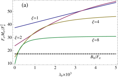
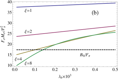
Figure 1: $F_{\sigma}M_{\sigma}$ in the unit of $F_{\pi}^{2}$ for $\xi=1,2,4,8$, $N_{h,c}=3$. $B_{0}/F_{\pi}$ is indicated as black dashed line. (a) $0\leq\lambda_{b}\leq 5\times 10^{-3}$ (b) $0\leq\lambda_{b}\leq 5\times 10^{-4}$.

and hence we obtain a relation (See fig. 2)

$$M_{\sigma\sigma}\simeq 5.0F_{\pi}\quad(\xi_{\sigma}\simeq 5),\quad F_{\sigma}\simeq 3.5F_{\pi}.$$ (42)

When we take a scale normalized by $L_{1}^{-1}=320~{}\text{MeV}$ so that we have $M_{V_{1}}=2.4/L_{1}=m_{\rho(770)}=770~{}\text{MeV}$, we obtain $F_{\pi}=87~{}\text{MeV}$, $M_{\sigma}\sim 450~{}\text{MeV}$ (fig. 2).

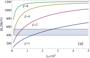
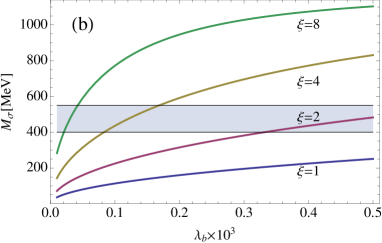
Figure 2: The lightest scalar mass as the sigma meson mass $M_{\sigma}$ v.s. scalar boundary coupling $\lambda_{b}$ with $\xi=1,2,4,8$, $N_{h,c}=3$, $L_{1}^{-1}=320~{}\text{MeV}$. The shaded band indicates the mass range of $f_{0}(500)$ PDG . (a) $0\leq\lambda_{b}\leq 5\times 10^{-3}$ (b) $0\leq\lambda_{b}\leq 5\times 10^{-4}$.

This result well agree with the experimental bound $400~{}\text{MeV}\leq m_{f_{0}(500)}\leq 550~{}\text{MeV}$ PDG , if we identify $f_{0}(500)$ as the sigma meson.

IV Hidden Pion Phenomenology

As a result of the previous sections, we now have three free parameters in this model: $M_{\pi},F_{\pi}$ and $v_{S}=v_{H}\tan\beta$. For numerical analysis, we scan the three-dimensional parameter space $(M_{\pi},F_{\pi},\tan\beta)$. Note that the SM-like Higgs boson with mass $125$ GeV is termed as $H$, and extra scalar particles as $H_{1}$ and $H_{2}$ with $M_{H1}<M_{H2}$. We have considered several theoretical and experimental constraints.

Let us first consider the theoretical constraints. From the stability of the potential, the dimensionless couplings should satisfy the relation,

$$\lambda_{HS}\leq\lambda_{H}\cdot\lambda_{S}~{}~{}{\rm with}~{}~{}\lambda_{H},\lambda_{S}>0,$$ (43)

which are translated into the following relation with the minimization conditions

$$\tan\beta\leq\sqrt{2}~{}\frac{M_{\pi}F_{\pi}}{v_{H}^{2}}.$$ (44)

Since the strongly interacting hidden sector are now treated as linear sigma model, the symmetry breaking condition in the $\sigma$-sector would constrain the value of $\mu^{2}_{\sigma}$ to be positive. With the help of eq. (10), the condition reads

$$M_{\pi}\leq\frac{\xi_{\sigma}F_{\pi}}{\sqrt{3}}.$$ (45)

We also adopt the perturbativity bound on $\lambda_{S}$ with our definition of the Lagrangian:

$$\lambda_{S}\leq\frac{4\pi}{3}.$$ (46)

Experimental constraints considered in the analysis are listed in the following:

• Signal strength for the SM Higgs boson Khachatryan:2014jba ; Aad:2015gba ,

  $$\hat{\mu}=1.00\pm 0.13~{}\text{\cite[cite]{\@@bibref{Authors Phrase1YearPhrase2}{Khachatryan:2014jba}{\@@citephrase{(}}{\@@citephrase{)}}}}.$$ (47)

• Bounds for extra scalar particles from the LEP Barate:2003sz and the LHC CMS:2012bea ; TheATLAScollaboration:2013zha ; ATLAS:2014aga .

• Relic density from Planck satellite Ade:2015xua .

  $$\Omega_{DM}h^{2}=0.1198\pm 0.0015.$$ (48)

• Neutrino signals through the DM capture by the Sun, mostly from Super-Kamiokande for upward muon flux Tanaka:2011uf .

• Fermi-LAT 6-year results for DM annihilation Ackermann:2015zua .

• Higgs invisible width from the LHC Aad:2014iia ; Chatrchyan:2014tja ,

  $${\rm Br}_{inv}\lesssim 0.51,~{}~{}{\rm with}~{}~{}95\%~{}{\rm C.L.}$$ (49)

• Direct detection bound, mostly from LUX Akerib:2013tjd , SuperCDMS Agnese:2014aze , and CRESST-II Angloher:2014myn .

We apply $2\sigma$ bounds with these experimental constraints except for the relic density, for which we use the measured value as an upper bound. This is because there could be additional contributions from hidden baryons to DM thermal relic density, which we do not include in this paper. We vary the $F_{\pi}$ up to 2 TeV and the ranges for $M_{\pi}$ and $\tan\beta$ are fixed with eq. (44) and eq. (45). We use micrOMEGAs Belanger:2013oya for evaluating DM-related observables.

The result of scanning is depicted in fig. 3. Here we see that there is definite lower bound for $F_{\pi}$, around 100 GeV. Also $\tan\beta$ is bounded from below, $\tan\beta\gtrsim 0.7$, mainly because of the perturbativity of $\lambda_{S}$ since it can be written in the form

$$\lambda_{S}=\frac{\lambda_{HS}}{\tan^{2}\beta}+\frac{2M_{\pi}^{2}F_{\pi}^{2}}{v_{H}^{4}\tan^{4}\beta}.$$ (50)

So if $\tan\beta$ is too small, $\lambda_{S}$ will have very large value, above the perturbativity bound. The island on the leftmost side are the solution points where $2M_{\pi}\sim M_{H}$, i.e. the SM-like Higgs resonances. Other points include light scalar resonanaces with $2M_{\pi}\sim M_{H1}$, heavy scalar resonances with $2M_{\pi}\sim M_{H2}$ and non-resonance solutions with $M_{H1}\ll 2M_{\pi}\ll M_{H2}$. The non-resonance solutions favor relatively small $\tan\beta$. For example, if the hidden pion mass is away from both resonance regions more than $30\%$, i.e. $1.3\cdot M_{H1}\leq 2M_{\pi}\leq 0.7\cdot M_{H2}$, then $\tan\beta$ is constrained to be smaller than about $3$. No points survive if the hidden pion mass is far away from the resonance regions, more than about $50\%$. This is because when $\tan\beta$ is small, the off-diagonal term of the mass matrix presented in eq. (5), $M^{2}_{hs}=-M_{hh}^{2}/\tan\beta$, is enhanced compared with large $\tan\beta$ case so that the mixing between the SM-like Higgs boson and singlet scalar fields are enhanced.

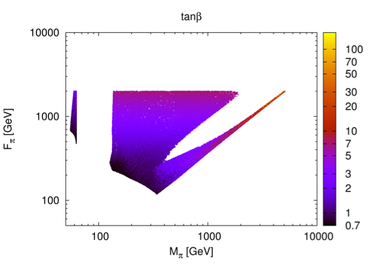
Figure 3: Solution points are shown in $(M_{\pi},F_{\pi})$ plane with color contours for $\tan\beta$.

These features for the solution points can be more easily checked with another forms of plots. In fig. 4, the solution points are shown in $(M_{\pi},M_{H1,H2})$ plane. The thin branch in the left plot is the collection of solution points where $M_{\pi}\sim M_{H1}/2$, light scalar resonances. Note that there is no solution points when $M_{H1}<M_{H}$, i.e. all extra scalar particles are heavier than the SM-like Higgs boson. The right plot, where the points are shown in $(M_{\pi},M_{H2})$ plane, also includes the thin branch that is corresponding to the solution points with heavy scalar resonances. The shape of the plot is almost same as fig. 3, since a relation $M_{H2}\sim\xi_{\sigma}F_{\pi}\sim 5F_{\pi}$ generally holds in this model. As a result, $M_{H2}$ has a definite lower bound ${\color[rgb]{0,0,0}M_{H2}\gtrsim 590~{}{\rm GeV}}$ as ${\color[rgb]{0,0,0}F_{\pi}\gtrsim 115~{}{\rm GeV}}$ does. Both plots also include the non-resonance cases, of which DM mass are far from both resonances and other parameters are tuned to satisfy the all constraints.

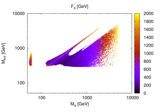
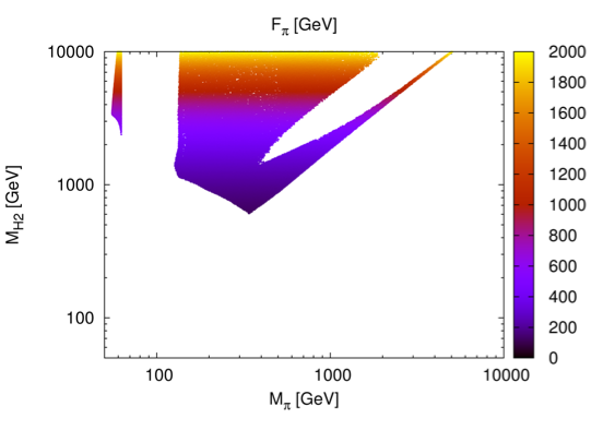
Figure 4: Solution points are shown in $(M_{\pi},M_{H1})$ plane (left) and $(M_{\pi},M_{H2})$ plane (right), with color contours for the hidden pion decay constant $F_{\pi}$.

As a distinctive observable, we show the deviation of the triple Higgs coupling from the SM prediction in fig. 5. The triple Higgs coupling in the model can reach $\sim 85\%$ of the SM prediction for relatively small $M_{\pi}$. If we take larger values for $M_{\pi}$ and $F_{\pi}$, it approaches to the SM one and cannot be a distinctive observable. Especially when $M_{\pi}$ is larger than 1 TeV, the triple Higgs coupling is very close to the SM prediction and the deviation cannot be detected.

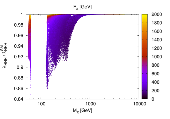
Figure 5: Triple Higgs couplings normalized with the SM values versus the hidden pion masses. Color contours represent the hidden pion decay constant $F_{p}i$.

Let us consider another observables. To be more specific, we separate the cases as the SM-like Higgs resonance and the other cases. fig. 6 shows the correlations between the Higgs signal strength $\hat{\mu}$ and DM-nucleon cross section in Higgs resonance case. Deviation of $\hat{\mu}$ from 1 is generated by the mixing angle $|V_{h0}|^{2}$ in eq. (13). In this case, the SM-like Higgs boson can decay to a pair of DM’s and these decay modes contribute to the Higgs invisible decay width. As one can see in the left plot, the invisible decay width of the SM-like Higgs boson increases when the signal strength decreases and vice versa, just like DM-nucleon cross section. We can understand this by the fact that the deviation of the signal strength is determined entirely by non-zero mixing angles among the SM-like Higgs and other extra scalar particles. The more they are mixed, the more wide the channel between the visible and hidden sector is open. We show in the right plot the same correlation with relic density contours. The variation of the relic density is caused by the small variation of $M_{\pi}$ and $F_{\pi}$ as long as $M_{\pi}$ is close to $\sim M_{H}/2$. In both plots we apply $2\sigma$ bound for the signal strength $\hat{\mu}$ such as $\hat{\mu}\geq 0.74$.

The same correlation is shown in fig. 7 for the other cases than the SM-like Higgs resonance. As mentioned before, the cases include light and heavy scalar resonances and non-resonance solutions. In this plot, the color contour represents the mass of the DM. Unlike the Higgs resonance case, relatively large values of the signal strength are favored, with generically larger values of DM-nucleon cross section. Note that there is an upper limit for $\hat{\mu}$. This bound is originated from the $h-\sigma$ mixing, that should be different from zero for avoiding the overclosure of the universe by the DM.

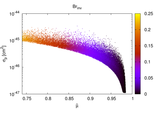
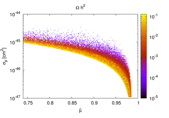
Figure 6: Correlation between the DM-nucleon cross sections and the Higgs signal strengths in the SM-like Higgs resonance cases. Color contours represent the SM-like Higgs invisible decay withs (left) and thermal relic density of the DM (right).

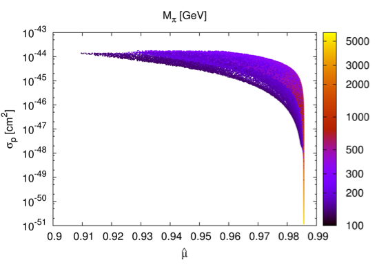
Figure 7: Correlation between the DM-nucleon cross sections and the Higgs signal strengths in resonance and non-resonance cases ,except the SM-like Higgs resonances. Color contours represent the hidden pion masses.

fig. 8 is showing the correlation between the signal strength and triple Higgs coupling normalized with the SM prediction. The left plot is for the SM-like Higgs resonance solutions and the right one for other cases. Both cases are predicting sharp linear correlations, but with different slopes. Two solution points are disjoint with each other, so the measurements of them can be used for the identification of the scenarios, though their values are small.

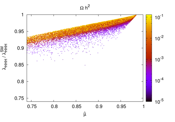
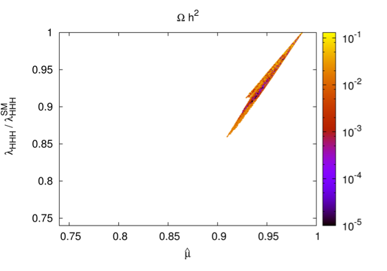
Figure 8: Correlations between the Higgs signal strength and triple Higgs couplings normalized with the SM values for the SM-like Higgs resonance (left) and the other cases (right). Color contours represent thermal relic densities.

Finally, some benchmark points are collected in Table 1. We classify the points as (A) SM Higgs resonance solutions, (B) light scalar resonances, (C) heavy scalar resonances, and (D) non-resonance solutions. The solution points with large relic densities (close to upper bound, $\Omega_{DM}^{exp}h^{2}\sim 0.1198$) are labelled as (I) and (II,III) correspond to the cases of small relic densities. Note that the closer we take the DM mass to the exact resonance, $M_{H}$ (or $M_{H1},M_{H2}$), the smaller the relic density becomes.

type	$F_{\pi}/{\tiny\rm GeV}$	$M_{\pi}/{\tiny\rm GeV}$	$\tan\beta$	$M_{H1}/{\tiny\rm GeV}$	$M_{H2}/{\tiny\rm GeV}$	$\Omega h^{2}$	$\sigma_{p}/{\tiny\rm cm^{2}}$	$\hat{\mu}$	${\rm BR_{Inv}}$	${\lambda_{HHH}}/{\lambda_{HHH}^{SM}}$
A-I	692.19	55.27	0.7881	346.281	3460.96	0.1220	$9.86\cdot 10^{-46}$	0.754	0.206	0.932
A-II	1524.33	62.49	1.648	415.13	7621.67	0.0027	$3.29\cdot 10^{-47}$	0.981	$3.8\cdot 10^{-4}$	0.994
B-I	1244.17	1000.08	4.288	2033.54	6224.10	0.1088	$2.88\cdot 10^{-49}$	0.986	0	1.000
B-II	1607.03	999.63	5.638	2000.65	8036.53	0.0101	$1.05\cdot 10^{-49}$	0.986	0	1.000
B-III	775.72	199.22	2.761	396.81	3878.60	0.0061	$4.92\cdot 10^{-47}$	0.984	0	0.998
C-I	227.49	549.85	1.479	570.38	1153.54	0.1193	$6.08\cdot 10^{-46}$	0.985	0	0.988
C-II	387.01	999.03	6.867	378.17	1938.82	0.0681	$2.07\cdot 10^{-47}$	0.985	0	1.000
D-I	185.66	319.49	1.337	323.97	930.67	0.1192	$4.94\cdot 10^{-45}$	0.964	0	0.965
D-II	208.73	231.86	0.906	405.30	1044.98	0.0101	$6.50\cdot 10^{-45}$	0.967	0	0.966

Table 1: Benchmark points for (A) SM-like Higgs resonance, (B) light scalar resonance, (C) heavy scalar resonance and (D) non-resonance cases.

V Summary and Conclusion

In this paper, we have analyzed the scale-invariant extension of the SM with vector-like confining gauge theory in the hidden sector by using the AdS/QCD proposed in Refs. DaRold:2005zs ; DaRold:2005vr . The model contains the singlet scalar field that connects the confining hidden sector and the scale-invariant SM sector. Hidden sector fermions develop nonzero chiral condensates and generate the linear term in the potential of the singlet scalar field $S$. As a result, the singlet scalar field $S$ develops a nonzero VEV and it provides the tachyonic mass term for the SM Higgs field. Therefore the origin of the EWSB in the SM sector lies in the new strong dynamics in the hidden sector.

We have used the AdS/QCD approach to describe non-perturbative dynamics of the hidden QCD sector. By the AdS/QCD, strongly interacting $SU(3)$ gauge theory in the hidden sector with two-flavors can be described by $SU(2)_{L}\times SU(2)_{R}$ gauge theory on $AdS_{5}$. The spectrum of the mesonic states then can be calculated up to overall scale by considering the two-point correlators. We first fixed the values of the AdS/QCD parameters that reproduce the known spectra of the mesons by identifying first KK mode of the vector state as rho meson. We applied the results to the hidden QCD. In this case, hidden rho meson mass is be treated as overall scale of the hidden QCD. By this, we successfully found out the relation between hidden sigma meson mass and hidden pion decay constant etc. As a result, we reduced the number of free parameters of the model to three, i.e. $F_{\pi},M_{\pi}$ and $\tan\beta$.

The hidden pions can be the DM candidates since the hidden sector flavor symmetry becomes an accidental symmetry of hidden sector strong interaction. We have analyzed these “hidden pion” properties as the DM. Many results of the DM search experiments were considered. In addition to the SM-like Higgs boson, we have two extra neutral scalar fields in the model. Those extended scalar sectors are constrained by the LHC data, for example Higgs signal strengths and non-observation of another scalar particles, etc. By scanning the three-dimensional parameter space $(M_{\pi},F_{\pi},\tan\beta)$, we found that the non-resonance solutions are also possible in addition to the resonance solutions. We also considered various correlations among the experimental observables. For example, there is the correlation between the Higgs signal strength $\hat{\mu}$ and DM-nucleon cross section, and also between $\hat{\mu}$ and the triple SM-like Higgs coupling. Especially for the latter, we found that their values and correlations behave differently depending on whether hidden pions have the SM-like Higgs resonance or not. Though the Higgs signal strength $\hat{\mu}$ has been measured quite precisely and seems to be consistent with the SM prediction, there is still room for the physics beyond the SM as discussed in this paper. If the Higgs signal strength $\hat{\mu}$ is measured more precisely, according to the sharp correlations we found, we can give peculiar predictions on the DM properties and others such as triple Higgs coupling etc. This could be seen in the benchmark points we presented at the end of the analysis.

Let us comment on the future prospects. Our model contains two extra neutral scalar bosons that mix with the SM-like Higgs boson. Mass spectra of those two scalar bosons are constrained by the up-to-date experimental results on the Higgs signal strengths in such a way that both of them are heavier than the 125 GeV SM-like Higgs boson. Besides the resonance solutions by the SM-like Higgs, extra light and heavy scalar particles, the non-resonance solutions are also possible for moderate values of hidden pion mass and decay constant. In that case, the mass of the light extra scalar particle will be around a few hundred GeV, which can be accessible at the LHC Run-II. The model also predicts the values of other observables such as relic density, DM-nucleon cross section and triple Higgs coupling and so forth. Especially, the Higgs signal strength $\hat{\mu}$ will be sharply determined. The more detailed study on the collider phenomenologies, for example, the pair production of the SM-like Higgs boson, could be possible. In addition, more complete studies with the hidden baryons, another DM candidates, can be pursued with the AdS/QCD.

Appendix A AdS/QCD formulas

Scalar meson mass $M_{S_{n}}$ and decay constant $F_{S_{n}}$ are obtained DaRold:2005vr by comparing the scalar correlator

$$\Pi_{S}(p_{E}^{2}) = \alpha^{2}M_{5}L\left[\frac{1}{L_{0}^{2}}+\frac{ip_{E}}{L_{0}}\frac{J_{0}(ip_{E}L_{0})+b(p_{E}Y_{0}Y_{0}(ip_{E}L_{0}))}{J_{1}(ip_{E}L_{0})+b(p_{E})Y_{1}(ip_{E}L_{0})}\right]$$ (51)

$$\stackrel{{\scriptstyle L_{0}\to 0}}{{\simeq}} \alpha^{2}M_{5}L\left[\frac{1}{L_{0}^{2}}+\frac{1}{2}p_{E}^{2}\ln(p_{E}^{2}L_{0}^{2})+\frac{\pi p_{E}^{2}}{2b(p_{E})}\right],$$ (52)

$$b(p_{E}) = -\frac{ip_{E}L_{1}J_{2}(ip_{E}L_{1})-\frac{8\lambda_{b}\xi^{2}}{M_{5}L}J_{1}(ip_{E}L_{1})}{ip_{E}L_{1}Y_{2}(ip_{E}L_{1})-\frac{8\lambda_{b}\xi^{2}}{M_{5}L}Y_{1}(ip_{E}L_{1})}$$ (53)

(where $p_{E}$ is the Euclidean momentum) with the correlator in Large-$N$ QCD

$$\Pi_{S}(p_{E}^{2}) = \sum_{n}\frac{F_{S_{n}}^{2}M_{S_{n}}^{2}}{p_{E}^{2}+M_{S_{n}}^{2}}.$$ (54)

The masses of scalar resonances are determined by finding the poles, $b(p_{E})=0$ or

$$M_{S_{n}}L_{1}J_{2}(M_{S_{n}}L_{1})=\frac{8\lambda_{b}\xi^{2}}{M_{5}L}J_{1}(M_{S_{n}}L_{1}),$$ (55)

and corresponding residues gives the scalar decay constants

$$F_{S_{n}}^{2} = \frac{3\tilde{N}_{c}\pi M_{S_{n}}^{2}(\frac{8\lambda_{b}\xi^{2}}{M_{5}L}Y_{1}(M_{S_{n}}L_{1})-M_{S_{n}}L_{1}Y_{2}(M_{S_{n}}L_{1}))}{M_{S_{n}}L_{1}(1-\frac{8\lambda_{b}\xi^{2}}{M_{5}L})J_{0}(M_{S_{n}}L_{1})+(\frac{8\lambda_{b}\xi^{2}}{M_{5}L}+M_{S_{n}}^{2}L_{1}^{2}-2)J_{1}(M_{S_{n}}L_{1})}.$$ (56)

References

- (1) G. Aad et al. [ATLAS Collaboration], Phys. Lett. B 716 (2012) 1 [arXiv:1207.7214 [hep-ex]].
- (2) S. Chatrchyan et al. [CMS Collaboration], Phys. Lett. B 716 (2012) 30 [arXiv:1207.7235 [hep-ex]].
- (3) C. T. Hill and E. H. Simmons, Phys. Rept. 381 (2003) 235 [Phys. Rept. 390 (2004) 553] [hep-ph/0203079].
- (4) F. Wilczek, Int. J. Mod. Phys. A 21 (2006) 2011 [physics/0511067].
- (5) M. E. Peskin and T. Takeuchi, Phys. Rev. Lett. 65 (1990) 964.
- (6) W. A. Bardeen, FERMILAB-CONF-95-391-T, C95-08-27.3.
- (7) T. Hur, D. W. Jung, P. Ko and J. Y. Lee, Phys. Lett. B 696 (2011) 262 [arXiv:0709.1218 [hep-ph]].
- (8) P. Ko, Int. J. Mod. Phys. A 23, 3348 (2008) doi:10.1142/S0217751X08042109 [arXiv:0801.4284 [hep-ph]].
- (9) P. Ko, AIP Conf. Proc. 1178, 37 (2009). doi:10.1063/1.3264554
- (10) P. Ko, PoS ICHEP 2010, 436 (2010) [arXiv:1012.0103 [hep-ph]].
- (11) T. Hur and P. Ko, Phys. Rev. Lett. 106 (2011) 141802 [arXiv:1103.2571 [hep-ph]].
- (12) M. Heikinheimo, A. Racioppi, M. Raidal, C. Spethmann and K. Tuominen, Mod. Phys. Lett. A 29, 1450077 (2014) [arXiv:1304.7006 [hep-ph]].
- (13) M. Heikinheimo, A. Racioppi, M. Raidal, C. Spethmann and K. Tuominen, Nucl. Phys. B 876, 201 (2013) [arXiv:1305.4182 [hep-ph]].
- (14) M. Holthausen, J. Kubo, K. S. Lim and M. Lindner, JHEP 1312, 076 (2013) [arXiv:1310.4423 [hep-ph]].
- (15) D. W. Jung and P. Ko, Phys. Lett. B 732, 364 (2014) [arXiv:1401.5586 [hep-ph]].
- (16) A. Salvio and A. Strumia, JHEP 1406, 080 (2014) [arXiv:1403.4226 [hep-ph]].
- (17) J. Kubo, K. S. Lim and M. Lindner, Phys. Rev. Lett. 113, 091604 (2014) [arXiv:1403.4262 [hep-ph]].
- (18) J. Kubo, K. S. Lim and M. Lindner, JHEP 1409, 016 (2014) [arXiv:1405.1052 [hep-ph]].
- (19) P. Schwaller, Phys. Rev. Lett. 115, no. 18, 181101 (2015) [arXiv:1504.07263 [hep-ph]].
- (20) Y. Ametani, M. Aoki, H. Goto and J. Kubo, Phys. Rev. D 91, no. 11, 115007 (2015) doi:10.1103/PhysRevD.91.115007 [arXiv:1505.00128 [hep-ph]].
- (21) J. Kubo and M. Yamada, PTEP 2015, no. 9, 093B01 (2015) [arXiv:1506.06460 [hep-ph]].
- (22) N. Haba, H. Ishida, N. Kitazawa and Y. Yamaguchi, Phys. Lett. B 755, 439 (2016) doi:10.1016/j.physletb.2016.02.052 [arXiv:1512.05061 [hep-ph]].
- (23) K. A. Meissner and H. Nicolai, Phys. Lett. B 648 (2007) 312 [hep-th/0612165].
- (24) R. Foot, A. Kobakhidze and R. R. Volkas, Phys. Lett. B 655 (2007) 156 [arXiv:0704.1165 [hep-ph]].
- (25) K. A. Meissner and H. Nicolai, Phys. Lett. B 660 (2008) 260 [arXiv:0710.2840 [hep-th]].
- (26) T. Hambye and M. H. G. Tytgat, Phys. Lett. B 659 (2008) 651 [arXiv:0707.0633 [hep-ph]].
- (27) R. Foot, A. Kobakhidze, K. L. McDonald and R. R. Volkas, Phys. Rev. D 77 (2008) 035006 [arXiv:0709.2750 [hep-ph]].
- (28) S. Iso, N. Okada and Y. Orikasa, Phys. Lett. B 676 (2009) 81 [arXiv:0902.4050 [hep-ph]].
- (29) S. Iso, N. Okada and Y. Orikasa, Phys. Rev. D 80, 115007 (2009) [arXiv:0909.0128 [hep-ph]].
- (30) M. Holthausen, M. Lindner and M. A. Schmidt, Phys. Rev. D 82 (2010) 055002 [arXiv:0911.0710 [hep-ph]].
- (31) L. Alexander-Nunneley and A. Pilaftsis, JHEP 1009, 021 (2010) [arXiv:1006.5916 [hep-ph]].
- (32) K. Ishiwata, Phys. Lett. B 710, 134 (2012) [arXiv:1112.2696 [hep-ph]].
- (33) J. S. Lee and A. Pilaftsis, Phys. Rev. D 86, 035004 (2012) [arXiv:1201.4891 [hep-ph]].
- (34) N. Okada and Y. Orikasa, Phys. Rev. D 85, 115006 (2012) [arXiv:1202.1405 [hep-ph]].
- (35) S. Iso and Y. Orikasa, PTEP 2013, 023B08 (2013) [arXiv:1210.2848 [hep-ph]].
- (36) T. Gherghetta, B. von Harling, A. D. Medina and M. A. Schmidt, JHEP 1302, 032 (2013) [arXiv:1212.5243 [hep-ph]].
- (37) M. Das and S. Mohanty, Int. J. Mod. Phys. A 28, 1350094 (2013) [arXiv:1111.0799 [hep-ph]].
- (38) C. D. Carone and R. Ramos, Phys. Rev. D 88, 055020 (2013) [arXiv:1307.8428 [hep-ph]].
- (39) V. V. Khoze and G. Ro, JHEP 1310, 075 (2013) [arXiv:1307.3764 [hep-ph]].
- (40) A. Farzinnia, H. J. He and J. Ren, Phys. Lett. B 727, 141 (2013) [arXiv:1308.0295 [hep-ph]].
- (41) O. Antipin, M. Mojaza and F. Sannino, Phys. Rev. D 89, no. 8, 085015 (2014) [arXiv:1310.0957 [hep-ph]].
- (42) M. Hashimoto, S. Iso and Y. Orikasa, Phys. Rev. D 89, no. 5, 056010 (2014) [arXiv:1401.5944 [hep-ph]].
- (43) C. T. Hill, Phys. Rev. D 89, no. 7, 073003 (2014) [arXiv:1401.4185 [hep-ph]].
- (44) J. Guo and Z. Kang, Nucl. Phys. B 898, 415 (2015) [arXiv:1401.5609 [hep-ph]].
- (45) S. Benic and B. Radovcic, Phys. Lett. B 732, 91 (2014) [arXiv:1401.8183 [hep-ph]].
- (46) M. Y. Binjonaid and S. F. King, Phys. Rev. D 90, no. 5, 055020 (2014) [Phys. Rev. D 90, no. 7, 079903 (2014)] [arXiv:1403.2088 [hep-ph]].
- (47) K. Allison, C. T. Hill and G. G. Ross, Phys. Lett. B 738, 191 (2014) [arXiv:1404.6268 [hep-ph]].
- (48) A. Farzinnia and J. Ren, Phys. Rev. D 90, no. 1, 015019 (2014) [arXiv:1405.0498 [hep-ph]].
- (49) G. M. Pelaggi, Nucl. Phys. B 893, 443 (2015) [arXiv:1406.4104 [hep-ph]].
- (50) A. Farzinnia and J. Ren, Phys. Rev. D 90, no. 7, 075012 (2014) [arXiv:1408.3533 [hep-ph]].
- (51) R. Foot, A. Kobakhidze and A. Spencer-Smith, Phys. Lett. B 747, 169 (2015) [arXiv:1409.4915 [hep-ph]].
- (52) S. Benic and B. Radovcic, JHEP 1501, 143 (2015) [arXiv:1409.5776 [hep-ph]].
- (53) J. Guo, Z. Kang, P. Ko and Y. Orikasa, Phys. Rev. D 91, no. 11, 115017 (2015) [arXiv:1502.00508 [hep-ph]].
- (54) S. Oda, N. Okada and D. s. Takahashi, Phys. Rev. D 92, no. 1, 015026 (2015) [arXiv:1504.06291 [hep-ph]].
- (55) K. Fuyuto and E. Senaha, Phys. Lett. B 747, 152 (2015).
- (56) K. Endo and K. Ishiwata, Phys. Lett. B 749, 583 (2015) [arXiv:1507.01739 [hep-ph]].
- (57) A. D. Plascencia, JHEP 1509, 026 (2015) [arXiv:1507.04996 [hep-ph]].
- (58) K. Hashino, S. Kanemura and Y. Orikasa, arXiv:1508.03245 [hep-ph].
- (59) A. Karam and K. Tamvakis, Phys. Rev. D 92, no. 7, 075010 (2015) [arXiv:1508.03031 [hep-ph]].
- (60) A. Ahriche, K. L. McDonald and S. Nasri, arXiv:1508.02607 [hep-ph].
- (61) Z. W. Wang, T. G. Steele, T. Hanif and R. B. Mann, arXiv:1510.04321 [hep-ph].
- (62) N. Haba, H. Ishida, R. Takahashi and Y. Yamaguchi, arXiv:1511.02107 [hep-ph].
- (63) K. Ghorbani and H. Ghorbani, JHEP 1604, 024 (2016) doi:10.1007/JHEP04(2016)024 [arXiv:1511.08432 [hep-ph]].
- (64) A. J. Helmboldt, P. Humbert, M. Lindner and J. Smirnov, arXiv:1603.03603 [hep-ph].
- (65) R. Jinno and M. Takimoto, arXiv:1604.05035 [hep-ph].
- (66) A. Ahriche, K. L. McDonald and S. Nasri, arXiv:1604.05569 [hep-ph].
- (67) A. Ahriche, A. Manning, K. L. McDonald and S. Nasri, arXiv:1604.05995 [hep-ph].
- (68) A. Das, S. Oda, N. Okada and D. s. Takahashi, arXiv:1605.01157 [hep-ph].
- (69) V. V. Khoze and A. D. Plascencia, arXiv:1605.06834 [hep-ph].
- (70) L. Da Rold and A. Pomarol, Nucl. Phys. B 721 (2005) 79 [hep-ph/0501218].
- (71) L. Da Rold and A. Pomarol, JHEP 0601, 157 (2006) [hep-ph/0510268].
- (72) K. A. Olive et al. [Particle Data Group Collaboration], Chin. Phys. C 38, 090001 (2014).
- (73) V. Khachatryan et al. [CMS Collaboration], Eur. Phys. J. C 75 (2015) 5, 212 [arXiv:1412.8662 [hep-ex]].
- (74) G. Aad et al. [ATLAS Collaboration], arXiv:1507.04548 [hep-ex].
- (75) R. Barate et al. [LEP Working Group for Higgs boson searches and ALEPH and DELPHI and L3 and OPAL Collaborations], Phys. Lett. B 565 (2003) 61 [hep-ex/0306033].
- (76) CMS Collaboration [CMS Collaboration], CMS-PAS-HIG-13-027.
- (77) The ATLAS collaboration [ATLAS Collaboration], ATLAS-CONF-2013-067, ATLAS-COM-CONF-2013-082.
- (78) G. Aad et al. [ATLAS Collaboration], Phys. Rev. D 92 (2015) 1, 012006 [arXiv:1412.2641 [hep-ex]].
- (79) P. A. R. Ade et al. [Planck Collaboration], arXiv:1502.01589 [astro-ph.CO].
- (80) T. Tanaka et al. [Super-Kamiokande Collaboration], Astrophys. J. 742 (2011) 78 [arXiv:1108.3384 [astro-ph.HE]].
- (81) M. Ackermann et al. [Fermi-LAT Collaboration], arXiv:1503.02641 [astro-ph.HE].
- (82) G. Aad et al. [ATLAS Collaboration], Phys. Rev. Lett. 112 (2014) 201802 [arXiv:1402.3244 [hep-ex]].
- (83) S. Chatrchyan et al. [CMS Collaboration], Eur. Phys. J. C 74 (2014) 2980 [arXiv:1404.1344 [hep-ex]].
- (84) D. S. Akerib et al. [LUX Collaboration], Phys. Rev. Lett. 112 (2014) 091303 [arXiv:1310.8214 [astro-ph.CO]].
- (85) R. Agnese et al. [SuperCDMS Collaboration], Phys. Rev. Lett. 112 (2014) 24, 241302 [arXiv:1402.7137 [hep-ex]].
- (86) G. Angloher et al. [CRESST-II Collaboration], Eur. Phys. J. C 74 (2014) 12, 3184 [arXiv:1407.3146 [astro-ph.CO]].
- (87) G. Belanger, F. Boudjema, A. Pukhov and A. Semenov, Comput. Phys. Commun. 185 (2014) 960 [arXiv:1305.0237 [hep-ph]].