Spatial neutral dynamics

Abstract

Neutral models, in which individual agents with equal fitness undergo a birth-death-mutation process, are very popular in population genetics and community ecology. Usually these models are applied to populations and communities with spatial structure, but the analytic results presented so far are limited to well-mixed or mainland-island scenarios. Here we present a new technique, based on interface dynamics analysis, and apply it to the neutral dynamics in one, two and three spatial dimensions. New results are derived for the correlation length and for the main characteristics of the community, like total biodiversity and the species abundance distribution above the correlation length. Our results are supported by extensive numerical simulations, and provide qualitative and quantitative insights that allow for a rigorous comparison between model predictions and empirical data.

Neutral dynamics, and the neutral models used to describe it, are one of the main conceptual frameworks in population biology and ecology Kimura (1985); Hubbell (2001); Azaele et al. (2015a). A neutral community is a collection of different populations, such as different species (in ecological models) or different groups of individuals with identical genetic sequence (haplotypes, for example, in population genetics). All individuals undergo a stochastic birth-death process, where in most of the interesting scenarios the overall size of the community, $J$, remains fixed or almost fixed. An offspring of an individual will be a member of its parent group with probability $1-\nu$, and with probability $\nu$ it mutates or speciates, becoming the originator of a new taxon. A neutral process does not include selection: all populations are demographically equivalent, having the same rates of birth, death and mutations, and the only driver of population abundance variations is the stochastic birth-death process (demographic noise).

A neutral dynamics is relevant, of course, to any inherited feature that does not affect the phenotype of an individual, such as a polymorphism in the non-coding part of the DNA or silent mutations, but many believe that its scope is much wider. In particular, the neutral theory of molecular evolution Kimura (1985) and the neutral theory of biodiversity Hubbell (2001) both suggest that even the phenotypic diversity observed in natural communities reflects an underlying neutral or almost-neutral process while the effect of selection is absent or very weak. Both theories have revolutionized the fields of population genetics and community dynamics, correspondingly, and despite bitter disputes, their influence is overwhelming.

For a well-mixed ($0$d) community the mathematical analysis of the neutral model is well-established, with the theory of coalescence dynamics Wakeley (2009) and Ewens’s sampling formula Ewens (1972) at its core. However, the species abundance distribution predicted by this model, the Fisher log-series, fails to fit the observed statistics of trees in a tropical forest. To overcome this difficulty, Stephen Hubbell suggested a simple spatial generalization of the neutral model, where a well mixed community on the mainland (a ”metacommunity”) is connected to a relatively small island by migration and immigrant statistics is given by Ewens’s sampling formula Hubbell (2001); Volkov et al. (2003). The abundance of a species on the island reflects the balance between its mainland abundance (assumed to be fixed, as variations on the mainland are much slower) and local stochasticity. The resulting island statistics depend on two parameters only, the combination $\theta=\nu J_{m}$ ($J_{m}$ is the mainland abundance) and $m$, the migration rate. The success of this two-parameter model in describing local communities, and its mathematical simplicity that allows for an exact solution in terms of zero-sum multinomials Volkov et al. (2003), were the key ingredients that contributed to the success of Hubbell’s neutral theory Rosindell et al. (2011); Azaele et al. (2015a).

Still, this mainland-island model is only an approximation. The tropical forest plots used to validate it are not ”islands” per se, instead they are arbitrary segments of very large forests on which a census takes place. Even the plot known as ”Barro-Colorado Island” is a $500\times 1000$m rectangle where the island area is $15.6km^{2}$. In practice there is no natural distinction between the local population and its surroundings and local dispersal ensures correlations between the two, correlations that have no analog in Hubbell’s mainland-island model. Consequently, one would like to have a solution, or at least a set of intuitive arguments, for the generic problem of spatially explicit neutral dynamics Ter Steege (2010). Several attempts have been made in this direction, both in the context of community ecology Zillio et al. (2005); Azaele et al. (2015b, a); O’Dwyer and Green (2010); De Aguiar et al. (2009); Rosindell and Cornell (2007) and in the context of population genetics Wilkins and Wakeley (2002).

The aim of this letter is to present a novel analysis, based on interface dynamics, of the spatial neutral model. Armed with this tool we can present expressions for the correlation length, species abundance distribution and species richness, and these expressions are shown to fit very nicely the results of extensive numerical simulations.

Technically speaking, the neutral dynamics is a ”technicolor” version of the well known voter model Liggett (2013). In the original voter model any individual has one of two colors, or opinions, and in an elementary timestep an agent is chosen at random to change its color, accepting instead the color of one of its randomly chosen neighbors. Such a game ends up, inevitably, with a fixation of the population by one color. A neutral game proceeds according to the same rules, with the exception that the agent accepts its neighbor’s opinion with probability $1-\nu$ and, with probability $\nu$, it becomes the originator of a new color (note that, unlike the two allele model considered by Korolev et al. (2010), in the infinite allele case considered here recurrent mutations are not allowed and a brand new species appears in every mutation).

Like the traditional voter model, the neutral dynamics may be analyzed using a ”backward in time” (coalescence) approach, becoming a coalescence random walk ($A+A\to A$) process Ben-Avraham and Havlin (2000). In its nearest-neighbor spatial version every individual selects its parent from one of its neighbors, and coalescence occurs when two agents choose the same parent. The resulting genealogic tree (in $1d$) is illustrated in Fig 1a, where lines representing ancestral relationships merge until the dynamics reaches the most recent common ancestor. Mutation/speciation events are represented by short thick lines that cut the lines, and all the leaves connected to a certain mutant by lines without mutations carry the same color, i.e, they belong to the same species. This property facilitates the simulation of a neutral dynamics Rosindell and Cornell (2007): instead of simulating the coalescence random walkers until the most recent common ancestor and then introducing random mutations with a chance proportional to the length of a line (number of birth), we have simulated coalescing and dying ($A\stackrel{{\scriptstyle\nu}}{{\longrightarrow}}\emptyset$) walkers, as depicted in figure 1b. Monitoring all descendent of an individual we were able to easily identify the colors of agents at $t=0$ (leaves) and to simulate a large system until it reaches the most recent relevant mutation (i.e., mutation that yields a currently existing species), avoiding the diverging timescales associated with the last coalescence events when only a few ancestors survive.

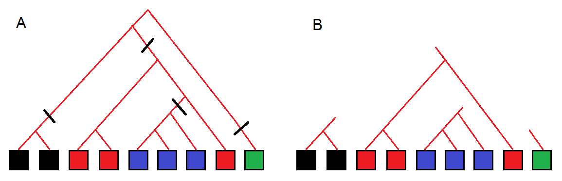
Figure 1: Two cartoons showing a possible genealogy and its corresponding neutral dynamics. In (A) the full genealogy of a $1d$ coalescence process with 9 individuals is presented. Every mutation (represented by thick dark lines cutting the line) generates a new species, and conspecific individuals at present have the same color. Panel (B) shows the same genealogy when simulated only until the last relevant mutation: coalescence history and mutations in the ”missing” part of the tree are irrelevant.

While implementing a backward in time approach for the numerics, our analytic arguments are based on the forward in time evolution of the system and focus on the interface area. To begin, let us consider the neutral dynamics in $1d$ (a model considered by geneticist, see Wilkins and Wakeley (2002)). Looking at a species represented by $x$ individuals (e.g., for the red species in Fig. 1, $x=3$, for the black $x=2$), one realizes that its dynamics is governed by two processes: weak losses at a rate $\nu x$ per generation due to mutations, and an unbiased diffusion in abundance space associated with the birth-death dynamics. Clearly, the strength of diffusion for $x$ is proportional to $I$, the interface between single color segments. For example, the red species in Fig. 1 has four interfaces, while for the blue one $I=2$. Assuming a narrow distribution of the number of interfaces around an average $I(x)$ (our simulations suggest a Poisson distribution), one may write a Fokker-Planck equation for the single species abundance dynamics,

$$\frac{\partial P(x,t)}{\partial t}=\frac{\partial^{2}[I(x)P(x,t)]}{\partial x^{2}}+\nu\frac{\partial[xP(x,t)]}{\partial x}$$ (1)

where $P(x,t)$ is the probability of a certain species to be represented by $x$ individuals at $t$ ($t$ is measured in generations). Once $I(x)$ is known, the equilibrium species abundance distribution (SAD) is given by,

$$P_{eq}(x)=\frac{e^{-\nu\int dx\frac{x}{I(x)}}}{I(x)}.$$ (2)

This formula is valid in any dimension, but $I(x)$ depends on dimensionality. To suggest an expression for $I(x)$, we introduce here a few arguments. The $1d$ case is discussed first, but some of the insights will be used below for higher dimensions.

First, the correlation length $\xi$ is defined via the chance of two individuals, at a distance $\ell$ apart, to have the same color. Having the backward picture in mind, this is equivalent to the chance that two random walkers, starting at a distance $\ell$ from each other, will coalesce before mutation occurs, i.e., within a time shorter than $1/(2\nu)$. The theory of first passage time Redner (2001) suggests that, for a nearest neighbors $1d$ dynamics, $\xi\sim 1/\sqrt{\nu}$. Accordingly, one should expect that species with $x>\xi$ will be rare (i.e., that $P_{eq}^{1d}(x)$ drops substantially above $\xi$) and that $I(x)$ scales linearly with $x$ for $x\gg\xi$, as the density of gaps becomes uncorrelated.

A second argument has to do with the overall species richness (SR). For a system of coalescing random walkers in one dimension the density of agents, $n(s)$ is known to fall like $n(s)=n(0)/\sqrt{s}$ Ben-Avraham and Havlin (2000). Here $s$ represents time, measured in generations, and we use $s$ instead of $t$ since in our case the coalescence picture is relevant when time is measured backward, starting with $n(0)=J$, the overall size of the community. The SR of a sample is given by integration over $s$, where in each generation one counts the number of agents that survived the coalescence-death process, $Je^{-\nu s}/s$, and multiplies it by the chance for mutation. The answer is $\nu$ times the volume of the ”truncated” tree shown in Figure 1b,

$$SR(J,\nu)\approx\nu J\int_{1}^{\infty}\frac{e^{-\nu s}}{\sqrt{s}}\ ds=B\sqrt{\nu}J$$ (3)

where $B$ is a constant of order unity.

On the other hand, $SR(J,\nu)$ is related to the SAD, $P_{eq}(x)$. The linear equation (1) yields a non-normalized SAD where normalization is determined by the condition $\int xP_{eq}(x)dx=J$. Accordingly Zillio et al. (2005),

$$SR(J,\nu)=B\sqrt{\nu}J=J\frac{\int_{1}^{\infty}P_{eq}(x)\ dx}{\int_{1}^{\infty}xP_{eq}(x)\ dx}.$$ (4)

A simple scaling argument shows that (if $P_{eq}$ is non-singular at zero) $P_{eq}$ is a function of $\sqrt{\nu}x$. Combining this with Eq. (2) and with the first argument, we suggest $I_{1d}(x)\sim 2+2B\sqrt{\nu}x{\cal F}(\sqrt{\nu}x)$ where ${\cal F}(z\gg 1)\to 1$.

Species with $x\ll\xi$ are quite compact. When a mutation occurs, it yields two interfaces that behave like two random walkers starting at $\ell=1$. If they survive until $t$ the corresponding species have abundance $x\sim\sqrt{t}$, so their genealogy is contained, more or less, within a triangle of base size $x$ and ”height” $x^{2}$. The chance of a mutation inside this triangle to occur $s$ generations before present is $\nu\sqrt{x^{2}-s}$, and it survives (hence adding two interfaces) with probability $1/\sqrt{s}$. Accordingly, the expected number of interfaces is given by $\nu\int_{0}^{x^{2}}ds\sqrt{(x^{2}-s)/s}\sim\nu x^{2}$ and we thus expect ${\cal F}(x\ll\xi)\to\sqrt{\nu}x$. Assuming further an exponential convergence to the $x>>\xi$ asymptotic value, one may guess a capacitor charging form

$$I_{1d}(x)=2+2B\sqrt{\nu}x\left(1-\exp(-A\sqrt{\nu}x)\right)$$

, with $A$ another constant. Plugging this into Eq. (2) one obtains,

$$P_{eq}^{1d}(x)=C\frac{e^{-\int\limits^{\sqrt{\nu}x}\frac{y\ dy}{2\left[1+By(1-exp(-Ay))\right]}}}{2\left[1+B\sqrt{\nu}x(1-exp(-A\sqrt{\nu}x))\right]}.$$ (5)

When $x\ll\xi$ the number of interfaces is almost fixed at two and the decay is Gaussian, but for large $x$ the decay switches to an exponential form. Figure 2 shows $P_{eq}^{1d}(x)$ for certain values of $\nu$, emphasizing the excellent fit and the data collapse when $P_{eq}^{1d}/\nu$ is plotted against $\sqrt{\nu}x$, where the constant was found to be $C=\nu J$.

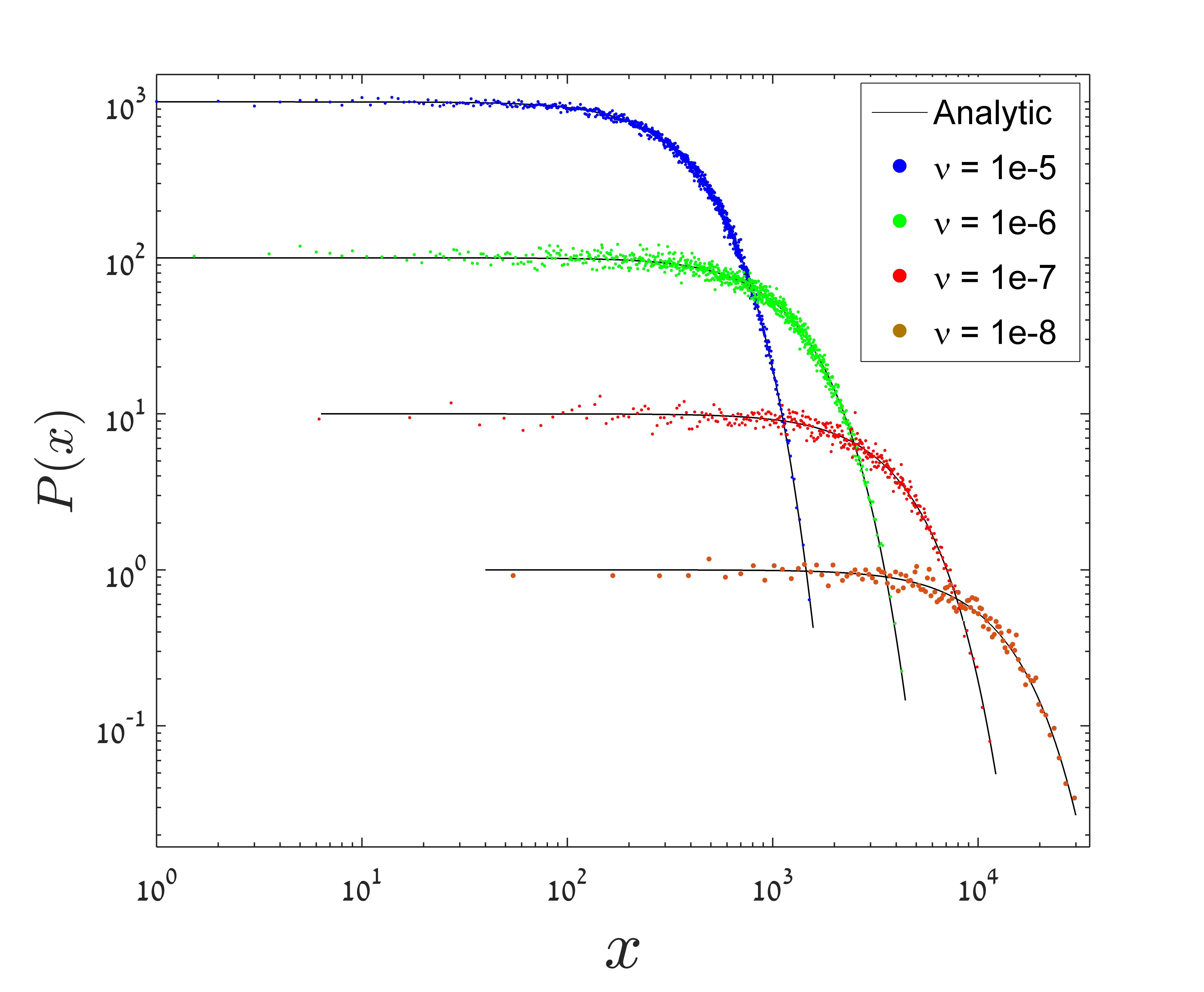
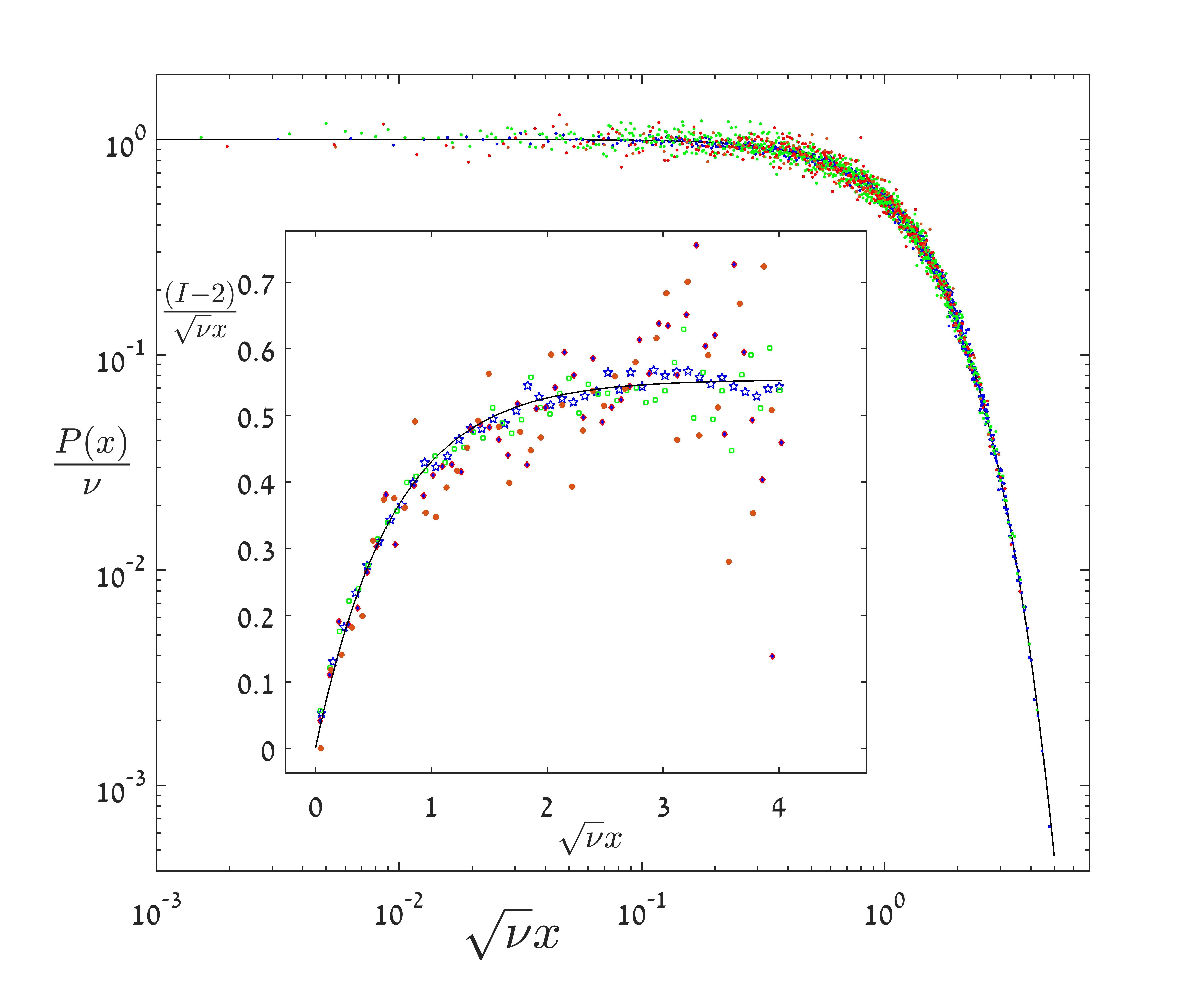
Figure 2: Species abundance distribution, $P(x)$ vs. $x$, for a $1d$ model with $J=10^{8}$ and different values of $\nu$, ranging from $\nu=10^{-5}$ to $10^{-8}$ (upper panel). The agreement with Eq. 5, with $A=1.5$ and $B=0.27$, is evident. In the lower panel $P(x)/\nu$ is plotted against $\sqrt{\nu}x$ for all datasets, and the perfect data collapse indicates that $P(x)$ is a function of $\nu{\cal G}(\sqrt{\nu}x)$, where ${\cal G}$ is a universal scaling function. The inset shows how $(I_{1d}(x)-2)/\sqrt{\nu}x$ scales with $\sqrt{\nu}x$, depicting the crossover from linear to saturation and the fit to the (full line) $\left(1-\exp(-A\sqrt{\nu}x)\right)$ (with the same value of $A$ for all $\nu$s). Datapoints for $x>\xi$ are rare, so the plot for these values is more noisy.

Establishing this intuitive framework by studying the $1d$ case, let us consider now the (much more important) $2d$ neutral model. Two is the critical dimension of the coalescing random walk problem Ben-Avraham and Havlin (2000); Krapivsky (1992) and of the first passage time in general Redner (2001), with logarithmic corrections to the mean field results, so one may expect that its analysis will be more difficult. This is probably true if the problem has to be solved exactly. However, for the analysis considered here the $2d$ model appears to be easier than its $1d$ counterpart.

Under a simple voter-model dynamics without mutations, the chance of the lineage of an individual to survive after $t$ generations goes like $ln(t)/t$ (as opposed to $1/t$ above $2d$) Krapivsky (1992). Accordingly, to keep the population fixed the average number of offspring of a surviving individual after $t$ generations has to be $t/ln(t)$. Therefore, up to logarithmic corrections, the age of a species with abundance $x$ is $t(x)\sim x\ln(x)$

Now, the neutral dynamics without mutation satisfies Eq. (1) with $\nu=0$. A simple scaling argument shows that to have $t\sim x\ln(x)$, $I_{2d}(x)=x/(1+c\ \ln(x))$, where $c$ is constant related to the amplitude of the kernel. Plugging this expression into Eq.(2) the SAD is found to be,

$$P_{eq}^{2d}=A\frac{1+c\ \ln(x)}{x}\exp\left(-\nu x[1+c(\ln(x)-1)]\right).$$ (6)

Figure 3 shows the excellent fits and data collapse this formula yields when $\nu$ varies over six decades, with $A=\nu J$. The species richness above $\xi$ is determined by Eq. (3); while the integration itself yields a complex expression, we find that

$$SR^{2d}(J,\nu)\sim J\nu[\ln(\nu)-1]^{2},$$ (7)

yields a decent approximation (maximum error of $15\%$ at $\nu=0.01$, converging to the correct result as $\nu$ becomes smaller). This expression also converges to $J$ when $\nu\to 1$.

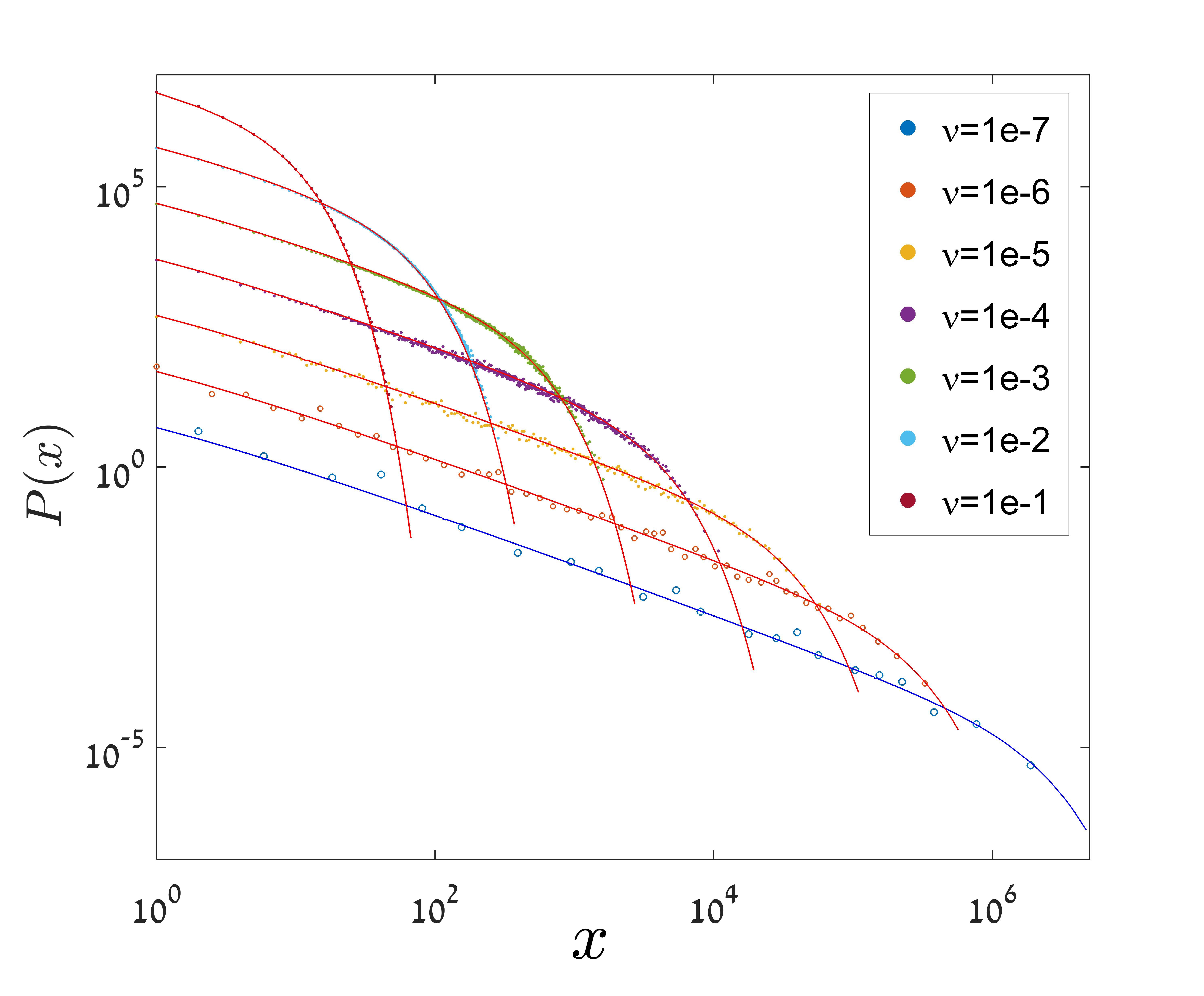
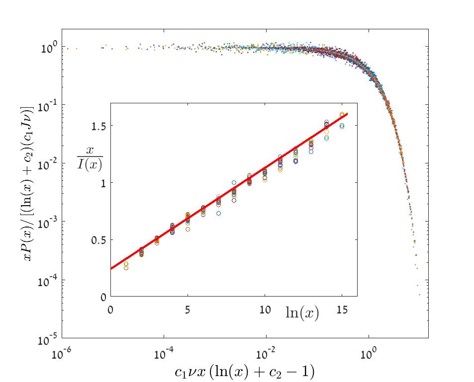
Figure 3: The upper panel shows the species abundance distribution, $P(x)$ as a function of $x$, for $\nu$ values between $10^{-1}$ to $10^{-7}$, together with fits to Eq. (6), with $c=0.36$. In the lower panel the data collapse obtained when $xP_{eq}/[1+c\ \ln(x)]$, for all these curves, is plotted against $\nu x[1+c(\ln(x)-1)]$. The inset shows $x/I(x)$ vs. $\ln(x)$ for $31$ runs from $\nu=10^{-8}$ to $\nu=10^{-1}$ (circles) and the full straight line indicates that $I(x)=x/(1+c\ \ln(x))$, with the same $\nu$ independent value of $c$. Datasets were collected from simulations of the backward in time process for systems of size $7000\times 7000$ ($J=4.9\cdot 10^{7}$) with a nearest neighbor dispersal kernel.

Above the critical dimension, $d>2$, the mean-field expressions of Galton-Watson theory describe accurately the dynamics at long times, meaning that the chance of the lineage of a new mutant to survive $t$ generations is $1/t$ and a surviving mutant has $t$ offspring. Accordingly, from Eq. 1 with $\nu=0$, $I(x)$ must scale linearly with $x$. This leads immediately to the celebrated Fisher log-series statistics,

$$P_{eq}^{d>2}=\frac{Ae^{-\nu x}}{x}.$$ (8)

This Fisher log-series has been implemented in the neutral models Hubbell (2001); Volkov et al. (2003) as the SAD on the mainland. In the relevant parameter regime the 2d SAD (6) and the mean field expression (8) differ strongly, both for frequent species (where the exponential decay is replaced by a factorial decay) and in the tail, where logarithmic corrections are important.

The results presented here disagree with the scaling analysis suggested in Zillio et al. (2005) (this scaling was already criticized in Pigolotti and Cencini (2009), where it failed to fit numerical results) . As one realizes from the backward in time exposition of the problem, the oldest species were originated about $1/\nu$ generations before present, and since every single lineage preforms an unbiased random walk, the largest distance between two conspecific individuals, which sets the correlation length, is of order $1/\sqrt{\nu}$, up to logarithmic corrections in $2d$. By the same token, the field theoretical analysis presented in O’Dwyer and Green (2010), and in particular the expression suggested for the species area curve (Eq. (10) of O’Dwyer and Green (2010)) are in contrast with our simulation results and with Eq. (7), as these authors predict a purely linear dependence of the SR on $\nu$, and a $\nu$ independent correlation length.

Our results, and in particular the universal characteristics of the community such as the functional dependence of species age on its abundance and the tail of the SAD, appear to be relevant for the new generation of large scale spatial surveys, like those presented recently for tropical forests Ter Steege et al. (2013); Slik et al. (2015). The data analysis in these works depends strongly on the assumption that the SAD is Fisher log-series; reinterpretation of these results in view of the spatially explicit model and its SADs presented here could be an enlightening exercise.

Acknowledgments We acknowledge the support of the Israel Science Foundation, grant no. $1427/15$.

References

- Kimura (1985) M. Kimura, The neutral theory of molecular evolution (Cambridge University Press, 1985).
- Hubbell (2001) S. P. Hubbell, The unified neutral theory of biodiversity and biogeography (MPB-32), vol. 32 (Princeton University Press, 2001).
- Azaele et al. (2015a) S. Azaele, S. Suweis, J. Grilli, I. Volkov, J. R. Banavar, and A. Maritan, arXiv preprint arXiv:1506.01721 (2015a).
- Wakeley (2009) J. Wakeley, Coalescent theory: an introduction, vol. 1 (Roberts & Company Publishers Greenwood Village, Colorado, 2009).
- Ewens (1972) W. J. Ewens, Theoretical population biology 3, 87 (1972).
- Volkov et al. (2003) I. Volkov, J. R. Banavar, S. P. Hubbell, and A. Maritan, Nature 424, 1035 (2003).
- Rosindell et al. (2011) J. Rosindell, S. P. Hubbell, and R. S. Etienne, Trends in ecology & evolution 26, 340 (2011).
- Ter Steege (2010) H. Ter Steege, Biotropica 42, 631 (2010).
- Zillio et al. (2005) T. Zillio, I. Volkov, J. R. Banavar, S. P. Hubbell, and A. Maritan, Physical review letters 95, 098101 (2005).
- Azaele et al. (2015b) S. Azaele, A. Maritan, S. J. Cornell, S. Suweis, J. R. Banavar, D. Gabriel, and W. E. Kunin, Methods in Ecology and Evolution 6, 324 (2015b).
- O’Dwyer and Green (2010) J. P. O’Dwyer and J. L. Green, Ecology letters 13, 87 (2010).
- De Aguiar et al. (2009) M. De Aguiar, M. Baranger, E. Baptestini, L. Kaufman, and Y. Bar-Yam, Nature 460, 384 (2009).
- Rosindell and Cornell (2007) J. Rosindell and S. J. Cornell, Ecology Letters 10, 586 (2007).
- Wilkins and Wakeley (2002) J. F. Wilkins and J. Wakeley, Genetics 161, 873 (2002).
- Liggett (2013) T. M. Liggett, Stochastic interacting systems: contact, voter and exclusion processes, vol. 324 (Springer Science & Business Media, 2013).
- Korolev et al. (2010) K. Korolev, M. Avlund, O. Hallatschek, and D. R. Nelson, Reviews of modern physics 82, 1691 (2010).
- Ben-Avraham and Havlin (2000) D. Ben-Avraham and S. Havlin, Diffusion and reactions in fractals and disordered systems (Cambridge University Press, 2000).
- Redner (2001) S. Redner, A guide to first-passage processes (Cambridge University Press, 2001).
- Krapivsky (1992) P. Krapivsky, Physical Review A 45, 1067 (1992).
- Pigolotti and Cencini (2009) S. Pigolotti and M. Cencini, Journal of theoretical biology 260, 83 (2009).
- Ter Steege et al. (2013) H. Ter Steege, N. C. Pitman, D. Sabatier, C. Baraloto, R. P. Salomão, J. E. Guevara, O. L. Phillips, C. V. Castilho, W. E. Magnusson, J.-F. Molino, et al., Science 342, 1243092 (2013).
- Slik et al. (2015) J. F. Slik, V. Arroyo-Rodríguez, S.-I. Aiba, P. Alvarez-Loayza, L. F. Alves, P. Ashton, P. Balvanera, M. L. Bastian, P. J. Bellingham, E. van den Berg, et al., Proceedings of the National Academy of Sciences 112, 7472 (2015).