Cusps in the center of galaxies: a real conflict with observations or a numerical artefact of cosmological simulations?

Abstract

Galaxy observations and N-body cosmological simulations produce conflicting dark matter halo density profiles for galaxy central regions. While simulations suggest a cuspy and universal density profile (UDP) of this region, the majority of observations favor variable profiles with a core in the center. In this paper, we investigate the convergency of standard N-body simulations, especially in the cusp region, following the approach proposed by (Baushev, 2015). We simulate the well known Hernquist model using the SPH code Gadget-3 and consider the full array of dynamical parameters of the particles. We find that, although the cuspy profile is stable, all integrals of motion characterizing individual particles suffer strong unphysical variations along the whole halo, revealing an effective interaction between the test bodies. This result casts doubts on the reliability of the velocity distribution function obtained in the simulations. Moreover, we find unphysical Fokker-Planck streams of particles in the cusp region. The same streams should appear in cosmological N-body simulations, being strong enough to change the shape of the cusp or even to create it. Our analysis, based on the Hernquist model and the standard SPH code, strongly suggests that the UDPs generally found by the cosmological N-body simulations may be a consequence of numerical effects. A much better understanding of the N-body simulation convergency is necessary before a ’core-cusp problem’ can properly be used to question the validity of the CDM model.

I Introduction

Results of N-body simulations come into increasing conflict with observations of the dark matter (DM) distribution in the central regions of dwarf galaxies. Astronomical observations favor relatively soft cored density profiles (Chemin et al., 2011; de Blok et al., 2001; de Blok and Bosma, 2002; Oh et al., 2011; Governato et al., 2012; Tollerud et al., 2012; Del Popolo and Pace, 2016). On the contrary, N-body simulations of cold dark matter tell us that dark matter halos have a universal shape, independent of the halo mass and initial density fluctuation spectrum, and that the central universal density profile (hereafter UDP) is cuspy. The first works on the subject proposed the Navarro-Frenk-White profile (hereafter NFW) that behaves as $\rho\propto r^{-1}$ at the center. Later simulations (Stadel et al., 2009; Navarro et al., 2010) favor the Einasto profile with a finite central density. However, the obtained Einasto index is so high (typically $n\sim 5-6$) that the profile is still cuspy and close to the NFW one.

For a time, there was a hope that the ’core-cusp problem’ would disappear once the baryon contribution is taken into account. However, recent simulations including baryon matter have rather amplified the problem (Oman et al., 2015): apart from the profile disagreement, a more fundamental difficulty was found. Of course, the presence of baryons in simulations changes the density profile, but it remains almost universal for all the halos, while the profiles of real galaxies are extremely varied. The conflict between simulations and observations might suggest that the cold DM paradigm is wrong. However, before reaching this conclusion, the accuracy and convergence of the simulations should be scrutinized. For instance, the overestimation of the energy exchange between the test bodies that may occur in the N-body simulations leads to the cusp formation (Baushev, 2014a). If the energy evolution during the halo formation is limited, then the density profile of the formed halo resembles more closely the observed one (Baushev, 2014b).

As an example, the overestimation of the particle energy exchange may be due to the unphysical pair collisions of the test bodies. Its importance may be characterized by the relaxation time (Binney and Tremaine, 2008, eqn. 1.32)

$$\tau_{r}=\dfrac{N(r)}{8\ln\Lambda}\cdot\tau_{d}$$ (1)

where $N(r)$ is the number of test bodies inside a sphere of radius $r$, $\ln\Lambda$ is the Coulomb logarithm, $\tau_{d}=(6\pi G\bar{\rho}(r))^{-1/2}$ is the characteristic dynamical time of the system at radius $r$, $\bar{\rho}(r)$ is the average density inside $r$. Equation 1 has two important consequences. First, $\tau_{r}$ depends on the smoothing radius of the N-body simulations only through $\Lambda$, i.e., only logarithmically (Baushev, 2015). Therefore, the influence of the unphysical collisional relaxation cannot be decreased much by the smoothing of the test body potentials. Second, since the number of dark matter particles is huge ($\sim 10^{60}$, if dark matter consists of elementary particles), the collisional relaxation plays no role in nature, being a purely numerical effect.

The algorithm stability is the critical point of N-body simulations: the Miller’s instability makes the Liapunov time comparable with the dynamical time of the system (Miller, 1964). Even if we take into account the specificity of N-body algorithms, like the potential smoothing, the instability development time is much shorter than $\tau_{r}$ and remains comparable with the dynamical time at the given radius $\tau_{d}(r)$ (Valluri and Merritt, 2000; Hut and Heggie, 2002). However, different N-body codes, with various versions of the Poisson solvers, integration algorithms etc., lead to final halos with the above-mentioned UDP, which is almost the same and close to NFW. Therefore, it is widely believed that the universal profile is physically meaningful and that it describes real halos, even though the orbits of individual test bodies have no physical significance (Binney and Tremaine, 2008, section 4.7.1(b)). The aim of this paper is to question this opinion.

Indeed, the convergency criteria of N-body simulations used at present are exclusively based on the density profile stability. (Power et al., 2003) found that the cusp of the UDP remains stable at least until $t=1.7\tau_{r}$ and then a core forms. On this basis (Power et al., 2003) supposed that the core formation is the first sign of the collision influence and offered the most extensively used criterion for simulation convergency $t<1.7\tau_{r}$. The acceptance that the collisions have no effect even if the simulation time exceeds $\tau_{r}$ seems surprising. However, later convergency tests (also based only on the stability of the density profile) suggested even softer criteria (Hayashi et al., 2003; Klypin et al., 2013). In this paper we perform a more sophisticated convergency test, going beyond the density profile analysis and considering the full array of the dynamical parameters of the particles.

II Calculations

II.1 The main idea

In order to test the N-body convergency, we follow the method offered in (Baushev, 2015). We simulate the well-known Hernquist model with the density profile $\rho(r)=Ma/[2\pi r(r+a)^{3}]$ (where $a$ is the scale radius and $M$ is the total halo mass), and with the isotropic velocity distribution at each point (Hernquist, 1990). The model is spherically symmetric and fully stable, i.e., the density and velocity profiles should not change with time. We chose the Hernquist model because it is close to the NFW and behaves exactly as the NFW ($\rho\propto r^{-1}$) in the central region, but it has a known analytical solution for the stationary velocity distribution, contrary to the NFW one. The region of the cusp ($r<a$) is of main concern to us.

Since the gravitational potential $\phi(r)$ is constant, the specific energy $\epsilon=\phi(r)+v^{2}/2$ and the specific angular momentum $\vec{K}$ of each particle should be conserved. Instead of $\epsilon$, it will be more convenient to use the apocenter distance of the particle $r_{0}$ (i.e. the maximum distance on which the particle can move off the center, which can be found from the implicit equation $\epsilon=\phi(r_{0})+K^{2}/2r_{0}$). Being an implicit function of the integrals of motion $\epsilon$ and $K$, $r_{0}$ is an integral of motion as well. Thus, any time variation of $\epsilon$, $\vec{K}$, or $r_{0}$ is necessarily a numerical effect, and we may judge the simulation convergency following the behavior of these quantities.

We need to clarify two important points of our work. Some properties of the perfectly symmetrical model we consider (like the exact conservation of the angular momentum for every particle) are unstable and not realistic for real astrophysical DM halos that are always triaxial as a result of tidal perturbations etc. The application of perfectly spherical models to real systems may give rise to false conclusions (Pontzen et al., 2015). However, the use of the spherical model for our purposes is well founded. We are not considering the task of comparison of simulation results with observations. Our aim is just to check if the ’N-body matter’ behaves as a collisionless matter, which is the principle question of the dark matter modelling.

Second, there is a frequent belief that it is much easier to converge on the spherically averaged density distribution than on the full properties of the phase space distribution function. Indeed, we need not correctly reproduce each individual particle trajectory. Moreover, it is not even necessarily desirable since real dark matter halos are not spherically symmetric and therefore host chaotic orbits. However, it would be completely wrong to disregard the phase evolution of the system or consider its evolution as a ’second order effect’ with respect to the density profile shape. As we will show in the Results: the simulation convergency section, correct simulations of the energy and angular momentum of each particle (contrary to individual particle trajectories) are of critical importance for correct simulations of the density profile.

Figure 1: The ratio between the time $t_{20\%}$ when the mass inside some radius $r$ drops on more than $20\%$, to the relaxation time $\tau_{r}(r)$.

II.2 The simulations

We simulate a single separate Hernquist halo. The aim of this work is to perform a sophisticated test of the standard convergency criteria, therefore we do not try to model any real astronomical object. Since the standard N-body units (Hénon, 1971) are used, the results are independent on the choice of $a$ and halo mass. However, we choose some values of the parameters, for illustrative purposes. Let us set $a=100$ pc, which roughly corresponds to the well-known dwarf spheroidal satellite of the Milky Way, Segue 1. This is one of the most popular objects for the indirect dark matter search, since it is close to the Solar System; its present-day mass can be estimated as $3\cdot 10^{7}M_{\odot}$ (Baushev et al., 2012). Segue 1 experienced strong tidal disruption, and we do not know its initial mass. We consider two limiting cases. In the body of the paper we accept the halo mass $M=10^{9}M_{\odot}$, which is comparable with the present-day mass of a larger dwarf satellite, Fornax (Walker and Peñarrubia, 2011) and almost certainly exceeds the initial mass of Segue 1. Thus we consider the case of a compact and very dense dwarf spheroidal galaxy. However, since all the simulations are performed in the dimensionless N-body units, a reader may easily extend the results for any value of $M$. If $a$ is fixed, the only value that is sensitive to the choice of $M$ is time: all the time intervals scale as $\Delta t\propto M^{-0.5}$ (while the ratios of time intervals remain the same). As an illustration, we also considered the case of $M=10^{7}M_{\odot}$, which is certainly lower, then the present-day mass of Segue 1. The only difference is that all the time intervals get ten times larger, and we everywhere specify the values corresponding to $M=10^{7}M_{\odot}$ in the footnotes. Anticipating events, we say that the results shown in all the figures in this paper are not sensitive at all to the choice of $M$.

We use $N=10^{6}$ test bodies . They are placed randomly, in accordance with the analytically obtained space and velocity distributions (Hernquist, 1990). The relaxation time at $r=a$ is $\tau_{r}(a)\simeq 8.8\cdot 10^{16}\text{s}\simeq 2.8\cdot 10^{9}$ years. Therefore, we make $200$ snapshots with the time interval $\Delta t=10^{15}\text{s}\simeq 30$ mln. years, covering the time from $0$ to $t_{max}=2\cdot 10^{17}\text{s}\simeq 6.5\cdot 10^{9}$ years (for the case of the halo mass $M=10^{7}M_{\odot}$, $\tau_{r}(a)\simeq 2.8\cdot 10^{10}$ years, $\Delta t=10^{16}\text{s}\simeq 300$ mln. years, $t_{max}=2\cdot 10^{17}\text{s}\simeq 6.5\cdot 10^{10}$ years). We record the positions and the velocities of each particle on each snapshot.

We evolve the system using one of the most extensively employed in cosmological simulations SPH codes, Gadget-3, an update version of Gadget-2 (Springel et al., 2001; Springel, 2005). The gravitational interactions in Gadget-3 are computed using a hierarchical tree (Barnes and Hut, 1986; Hernquist and Katz, 1989). In this algorithm the space is divided in different cells and the gravitational force acting on a particle is computed using a direct summation for particles that are in the same cell and by means of multipole (up to the quadrupole) expansion for the particles that are in a different cell. The minimum distance between particles to be part of a different cell is controlled by a tree opening criterion. Gadget-3 uses the Barnes-Hut tree opening criterion for the first force computation. This criterion is controlled by an opening angle $\mu$, which determines the maximum ratio between the distance to the center of mass of the cell ($d$) and the size of the cell ($l$). If the cell is too close to the particle, $d/l$ will be greater than $\mu$, and new cells have to be opened to maintain the accuracy on the force computation. In the further evolution of the system a dynamical updating criterion (controlled by the fractional error $f_{acc}$) is used. We use the standard set of parameters $\mu=0.7$ and $f_{acc}=0.005$, as suggested by (Springel, 2005; Springel et al., 2008; Boylan-Kolchin et al., 2009). These values lead to a relative force error that is roughly constant in the simulation $\sim 0.5$%. We chose the softening radius $0.02a=2$ pc, in accordance with (van Kampen, 2000; Hayashi et al., 2003).

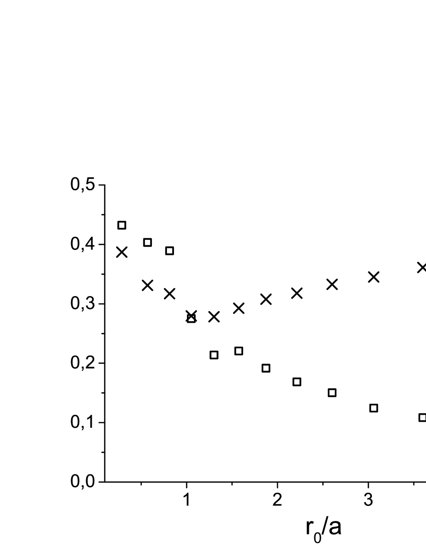
Figure 2: The averaged relative variations $\langle\widehat{\Delta}K/K_{circ}\rangle$ (squares) and $\langle\widehat{\Delta}r_{0}/r_{0}\rangle$ (crosses) of the integrals of motion in a single time step $\Delta t$. See the definition of the averaging $\widehat{\Delta}$ in the section Results: the integrals of motion.

III Results: the integrals of motion

Initially we convert each of the $201$ snapshots into the center-of-mass frame of references at the moment when a snapshot is made.

First of all, we try to reproduce the results of (Power et al., 2003). The density profile indeed remains quite stable, and then a core in the center appears. Exactly following (Power et al., 2003), we consider the moment $t_{20\%}$ when the mass inside some radius drops on $20\%$ comparing to the initial value as the moment of the core formation. The ratio of $t_{20\%}$ to the relaxation time $\tau_{r}$ at the same radius $r$ is represented in Fig. 1. We see that our data by and large confirm the results of (Power et al., 2003), the core really appears at $t\simeq 2\tau_{r}$.

Before proceeding any further, two important comments relating to all the subsequent text should be made. First, our convergency tests are mainly oriented on the radius interval $[0.25a;1.5a]$ where they are the most precise. This choice of the working interval might appear strange at first sight: typically the convergency problems occur much closer to the halo center. However, if we had chosen a realistic area $(r\leq 0.01a)$, then it would have contained only $\sim 100$ test particles, and the statistic would have been poor. On the other hand, the density profile between $0.25a$ and $0.75a$ remains much the same as in the center, since a power-law profile $\rho\propto r^{-1}$ is self-similar. The lower border of the region under consideration $r=0.25a$ is defined by our choice of the timestep $\Delta t=10^{15}$ s (for the case of the halo mass $M=10^{7}M_{\odot}$, $\Delta t=10^{16}\text{s}\simeq 300$ mln. years). At $r=0.1a$, $\tau_{r}\simeq\Delta t$, and the Hernquist profile is certainly corrupted by the collisions even on the first timestep. However, as we will see from the discussion of fig. 4, the core formation becomes visible in phase portrait at much larger distances than in the density profile itself. Therefore, only the results related to $r\geq 0.25a$ can be totally trusted.

Second, we want to consider variations of the integrals of motion as a function of radius. However, each particle contributes to the density profile on an interval between its pericenter radius $r_{min}$ and apocenter radius $r_{0}$. Hereafter we will consider $r_{0}$ as the characteristic radius corresponding to the particle. Indeed, if the particle orbit is elongated, the particle spends almost all the time near the apocenter, in accordance with the Kepler’s second law. On the contrary, if the orbit is circular, the particle moves along almost uniformly, but its radius always remains close to $r_{0}$.

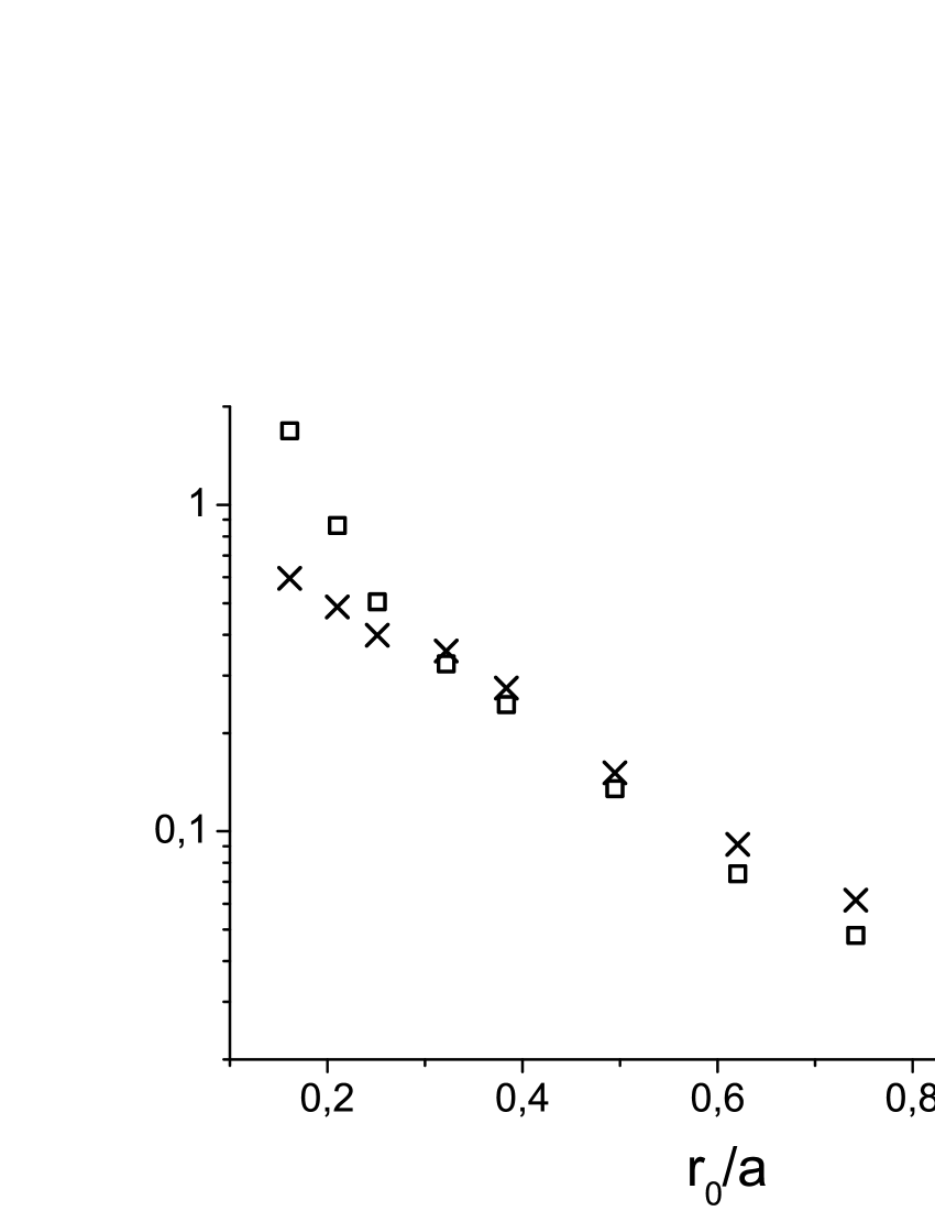
Figure 3: The ratios $\frac{K_{circ}}{\tau_{r}}\left\langle\frac{\widehat{\Delta}K}{\Delta t}\right\rangle^{-1}$ (squares) and $\frac{1}{\tau_{r}}\left\langle\frac{\widehat{\Delta}r_{0}}{r_{0}\Delta t}\right\rangle^{-1}$ (crosses) of the time, in which the particles completely ’forget’ the initial values of the integrals of motion, to the relaxation time $\tau_{r}(r)$.

In order to study the behavior of the integrals of motion (theoretically they should conserve), we order all $10^{6}$ particles according to their $r_{0}$ in the initial snapshot, and then divide the particles into 200 groups of 5000 particles each. All the particles in the same group have similar $r_{0}$, and the group may be characterized by the average initial $\overline{r_{0}}$ of its members. We calculate $\Delta r_{0}/r_{0}=(r_{0}(i+1)-r_{0}(i))/r_{0}$ and $\Delta K/K_{circ}=(K(i+1)-K(i))/K_{circ}$ for each particle on each timestep. Here $i$ is the number of the snapshot, $K_{circ}$ is the angular momentum corresponding to the circular orbit at $r_{0}$; apparently, this is the maximum value of $K$ any particle with the apocenter distance $r_{0}$ may possess. Then we find the root-mean-squares of $\Delta r_{0}/r_{0}$ and $\Delta K/K_{circ}$ averaged over each group and for each snapshot. Our analysis shows that the root-mean-squares do not significantly depend on time until the moment when the core forms at the radius corresponding to $\overline{r_{0}}$ of the group. Therefore, we then average the root-mean-squares of $\Delta r_{0}/r_{0}$ and $\Delta K/K_{circ}$ over all the timesteps where the core had not formed yet. We denote the values averaged in such a complex manner by $\langle\widehat{\Delta}r_{0}/r_{0}\rangle$ and $\langle\widehat{\Delta}K/K_{circ}\rangle$.

The dependance of $\langle\widehat{\Delta}K/K_{circ}\rangle$ (squares) and $\langle\widehat{\Delta}r_{0}/r_{0}\rangle$ (crosses) from the dimensionless radius $\overline{r_{0}}/a$ is represented in Fig. 2. We see that even in a single time step $\Delta t=10^{15}\text{s}\simeq 30$ mln. years (for the case of the halo mass $M=10^{7}M_{\odot}$, $\Delta t=10^{16}\text{s}\simeq 300$ mln. years) the integrals (that should be constant) vary significantly. Fig. 3 represents the values $\frac{K_{circ}}{\tau_{r}}\left\langle\frac{\widehat{\Delta}K}{\Delta t}\right\rangle^{-1}$ (squares) and $\frac{1}{\tau_{r}}\left\langle\frac{\widehat{\Delta}r_{0}}{r_{0}\Delta t}\right\rangle^{-1}$ (crosses) that are the ratios of the time intervals in which an average particle totally ’forgets’ its initial values of $K$ and $r_{0}$ to the relaxation time $\tau_{r}(r)$. Everywhere in the region of reliability ($r\geq 0.25a$) the ratios are much less than $1$.

It means that the particles totally ’forget’ their integrals of motion in a time much shorter than $\tau(r)$. In general one could not expect a reliable simulation of the velocity distribution at $t\sim\tau(r)$ under such conditions.

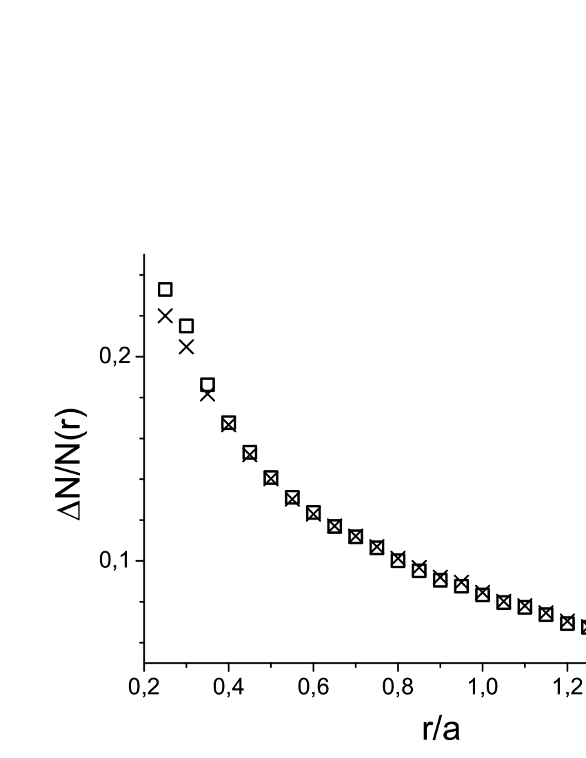
Figure 4: The upward $\Delta N_{+}(r)/\Delta t$ (squares) and downward $\Delta N_{-}(r)/\Delta t$ (crosses) Fokker-Planck streams of particles divided by the total number of the particles $N(r)$ inside $r$.

IV Results: the simulation convergency

Thus, the integrals of motion of the particles are not conserved at all, while the density profile remains stationary in quite good agreement with the theory in our simulations (we should mention, however, that the absence of the collision influence up to almost $2$ relaxation times looks surprising (Baushev, 2015). The same stability and reproducibility of the cusps in cosmological modelling leads to the wide acceptance of the idea that, though no significance can be attached to the trajectories of individual particles in the N-body simulations, the cuspy density profile is meaningful and should correctly describe the profiles of real halos. Let us use our results to illustrate the vulnerability of the profile stability as the only convergency criterion of the N-body simulations.

Indeed, if a Hernquist halo consists of real DM (we suppose that it is cold and noninteracting), the values of $\epsilon$, $\vec{K}$, and $r_{0}$ of each particle must conserve, the particle distribution function $f$ should depend only on $\epsilon$ and $K$ (Binney and Tremaine, 2008) and obey the collisionless kinetic equation $df/dt=0$. It means that there are no particle fluxes in the phase space $(\epsilon,K)$.

However, figures 2 and 3 doubtlessly reveal an intensive energy and angular momentum exchange between the particles, i.e., the test bodies interact. Then the system may be described by the Fokker-Planck (hereafter FP) equation (Landau and Lifshitz, 1980)

$$\dfrac{df}{dt}=\frac{\partial}{\partial q_{\alpha}}\left\{{\tilde{A}_{\alpha}}f+\frac{\partial}{\partial q_{\beta}}[B_{\alpha\beta}f]\right\}$$ (2)

where $q_{\alpha}$ is an arbitrary set of generalized coordinates,

$${\tilde{A}_{\alpha}}=\dfrac{\overline{\delta q_{\alpha}}}{\delta t}\qquad B_{\alpha\beta}=\dfrac{\overline{\delta q_{\alpha}\delta q_{\beta}}}{2\delta t}$$ (3)

We may choose $q_{1}=\epsilon$, $q_{2}=K$, and figure 2 shows that at least coefficients $B_{11}$ and $B_{22}$ in the equation (2) differ essentially from zero. Thus we model real DM halos that are believed to be collisionless, by a system of test bodies governed by the kinetic equation with a significant collisional term, i.e., by an essentially collisional equation.

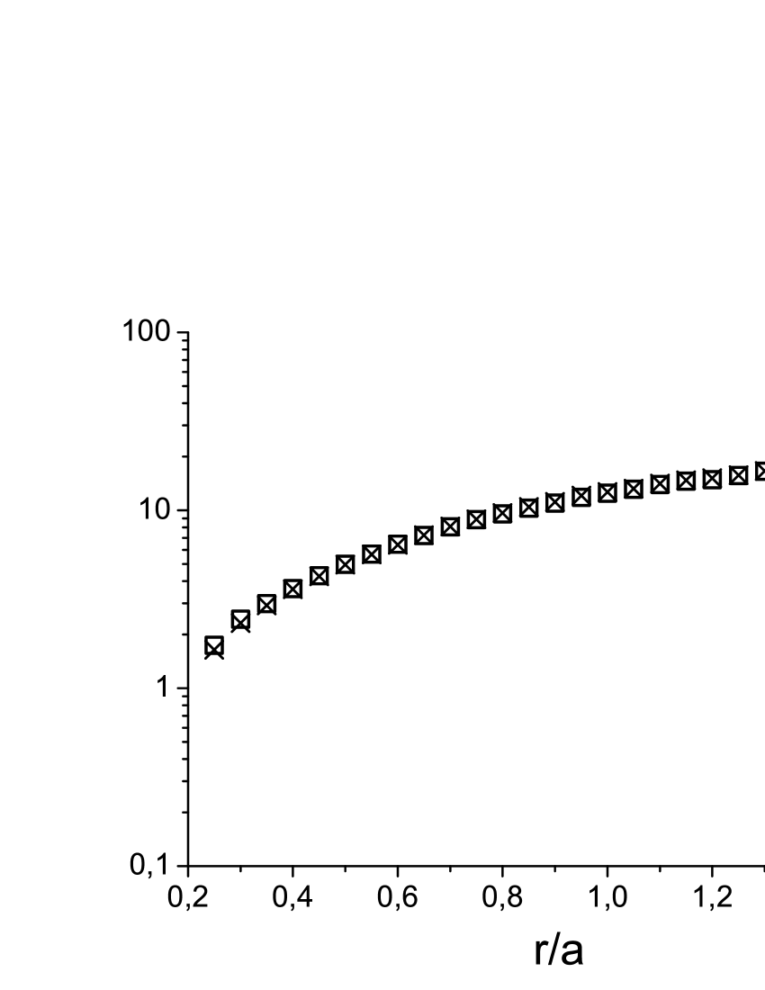
Figure 5: The fractions of $N(r)$ particles inside radius $r$ that is carried away and in by the upward and downward Fokker-Planck streams in the time $1.7\tau_{r}$ offered by (Power et al., 2003) ($1.7\tau_{r}\frac{\Delta N_{+}(r)}{N(r)\Delta t}$ (squares) and $1.7\tau_{r}\frac{\Delta N_{-}(r)}{N(r)\Delta t}$ (crosses), respectively).

An important point must be underscored: the density profile in our simulation indeed holds its shape (close to the NFW one in the center), in gratifying agreement with the theoretical predictions. The variations of the integrals of motion, that we found, mainly touches on the velocity distribution of the particles. Together with the UDP stability in cosmological simulations, it can produce a dangerous illusion that N-body simulations might adequately model the density profiles of dark matter structures, despite the fact that the velocity distribution was distorted. We should emphasize that it cannot be true. Indeed, let us consider a stationary spherically symmetric halo for the sake of simplicity. The particle distribution in the phase space $fd^{3}xd^{3}v$ is a function of only the particle energy $\epsilon$ and three components if its angular momentum $\vec{K}$ (Binney and Tremaine, 2008). If the velocity distribution of the particles is anisotropic in each point (which is the case under consideration in this paper), $f$ depends only on the particle energy $f(ep)=f(\phi(r)+v^{2}/2)=f(\phi(r_{0})+K^{2}/(2r_{0}^{2}))$. The particle speed distribution at some radius $r$ is therewith equal to $4\pi v^{2}f(\phi(r)+v^{2}/2)dv$, and the density is $\int 4\pi v^{2}f(\phi(r)+v^{2}/2)dv$. These relationships clearly demonstrate the impossibility of a reliable determination of the density profile without a reliable determination of the velocity distribution. The distributions over $\vec{v}$ and $r$ are not just bound, there are actually a sort of projections of the same distribution $f$ on the velocity or space coordinates. Apparently, this conclusion is very general and does not depend on the assumption about the spherical symmetry that we made.

We are able to compare the results with the theoretical prediction and check their agreement in the model case that we consider. However, it is impossible in the case of real cosmological simulations. Therefore, any numerical effect influencing on the velocity distribution $f(\vec{v})$ or on the integrals of motion of the test particles puts the density profiles obtained in the simulations in doubt. Moreover, the fact that the cuspy profile $\rho\propto r^{-1}$ turns out to be very stable in our simulation, despite of $r_{0}$ and $K$ variations, is probably not a coincidence, but a direct result of the numerical effects we discuss.

Indeed, the fact that we model collisionless systems with the test bodies governed by an essentially collisional equation is surprising per se, but the main consequence is that the profile stability does not guarantee the simulation correctness. The FP streams in the phase space created by the particle interaction may form stable density profiles (corresponding to the stationary solutions of the Fokker-Planck equation), but these profiles and their persistence are at odds with the behavior of real collisionless systems. As the first and crude illustration, the collisions lead to the contraction of the central region of any realistic profile and finally to the core collapse. The density profile outside the core approaches a power law $\rho\propto r^{-2.23}$ and then remains quite stable for a long time (Binney and Tremaine, 2008). Of course, this distribution is already formed by the unphysical test body collisions, and the immutability of the $\rho\propto r^{-2.23}$ profile says nothing either about the simulation convergency or about the behavior of real collisionless systems.

The core collapse appears at $t\gg\tau_{r}$ and has nothing to do with the Hernquist or the UDP profiles. However, the Fokker-Planck equation has an another stationary solution close to the NFW one (Evans and Collett, 1997; Baushev, 2015).

A question appears: if we obtain a stable cuspy density profile, how can we differentiate cusps correlating with the properties of real collisionless systems from the solutions created by the numerical effects? In a collisionless system, the values of $r_{0}$ of the particles in the cusp should remain constant. If collisions are significant, the values of $r_{0}$ should experience a random walking, and the particles move up and down in the cusp forming a downward stream (of the particles with decreasing $r_{0}$) and an upward stream (of the particles with increasing $r_{0}$). For the cusp to be stable, the streams should compensate each other, which corresponds to a stationary solution of the Fokker-Planck equation. Thus, if the cusp is created by the FP diffusion, we should see two significant streams of particles with decreasing and increasing $r_{0}$, and the streams should compensate each other in order to provide the cusp stability.

We chose two adjacent (i.e., divided by a single $\Delta t$) snapshots at the beginning of the simulations, in order to minimize the core formation effects. For an array of radii $r$, we calculated the number $\Delta N_{+}(r)$ of particles that had $r_{0}<r$ at the first snapshot and $r_{0}>r$ at the second one, and the number $\Delta N_{-}(r)$ of particles that had $r_{0}>r$ at the first snapshot and $r_{0}<r$ at the second one. Of course, $\Delta N_{+}(r)=\Delta N_{-}(r)=0$ in the collisionless case, since $r_{0}$ is an integral of motion.

Fig. 4 represents $\Delta N_{+}(r)$ (squares) and $\Delta N_{-}(r)$ (crosses) divided by the total number of the particles $N(r)$ inside $r$. As we can see, the FP streams exist, though they compensate well each other outside of $r=0.4a$. As we approach the center, the upward stream becomes increasingly stronger than the downward one. This is the first sign of the core formation, that is still invisible in the density profile at this radius, being already quite clear at the phase picture of the system.

A question appears: are the discovered fluxes $\Delta N_{+}(r)$ and $\Delta N_{-}(r)$ real and important? May they be just a small noise, produced by particles near the boundary, crossing and recrossing it and thus giving the impression of flows that do not exist? One can readily see that this is not the case. First of all, $\Delta N_{+}(r)$ and $\Delta N_{-}(r)$ apparently give only the lower bounds on the upward and downward FP streams: the value of $r_{0}$ of a particle could have crossed $r$ an odd number of times (and then it is counted only once) or an even number of times (and then it is not counted at all). Since we count each particle no more than once on a timestep, we totaly avoid the recrossing effect.

Second, the flows are just too strong to be just a noise. For instance, Fig. 4 shows that, though $\Delta N_{+}(r)$ and $\Delta N_{-}(r)$ are just the lower bounds on the streams, $\Delta N_{+}(r)\simeq\Delta N_{-}(r)\simeq 2\cdot 10^{4}$ at $r=a$, i.e. $\sim 2\%$ of the total halo mass crosses this radius because of this unphysical effect on each timestep. This is approximately the total number of particles in the layer of thickness $\sim a/12$ around the radius $r=a$. The value $a/12$ by far exceeds the smoothing radius or any reasonable numerical noise that may occur in the computing scheme.

The surprisingly high intensity of the Fokker-Planck diffusion is the main result of this work. Approximately $8\%$ of particles are renewed even inside $r=a$. It means that in only $10\Delta t\simeq 300$ mln. years (for the case of the halo mass $M=10^{7}M_{\odot}$, $10\Delta t\simeq 3\cdot 10^{9}$ years), i.e., in $~{}5\%$ of the simulation time, all the particles inside the sphere $r=a$ (which contains a quarter of the total mass of the system) can be substituted by a purely numerical effect. The fractions of particles inside radius $r$ that can be carried away or in by the upward and downward Fokker-Planck streams in the Power’s time $1.7\tau_{r}$ are $1.7\tau_{r}\frac{\Delta N_{+}(r)}{N(r)\Delta t}$ and $1.7\tau_{r}\frac{\Delta N_{-}(r)}{N(r)\Delta t}$. Fig. 5 shows that they always significantly exceed $1$. The cusp in our simulations was created in the initial conditions, but its shape is similar to the UDP. We can see that the unphysical FP streams are strong enough to arbitrarily change the shape of the cusp (and therefore the shape is defined by the FP diffusion rather than by the properties of the collisionless system) and even to create it.

Another argument in support of the numerical nature of the cusps in cosmological simulations is the profile universality. The similarity contradicts the observational results (Oman et al., 2015), but is quite natural if the cusps are formed by the FP diffusion. An UDP-like stationary solution is innate for the FP equation: the suppositions in (Evans and Collett, 1997) and (Baushev, 2015) are quite different, but the results are similar. The properties of the solution of the FP equation are totally defined by only a few coefficients $\tilde{A}_{\alpha}$ and $B_{\alpha\beta}$ that can be similar for different N-body codes using similar algorithms, and are almost certainly the same within the same simulation. As a result, the resulting halos are also self-similar, while nature is much more variable.

The second important conclusion of this section is that the profile stability cannot be used as the simulation convergency criterion: the first unquestionable signs of the influence of the test particle interaction appear in the phase portrait much earlier than the density profile evolution and the beginning of the core formation.

The third conclusion is that, since the variations of $K$ and $r_{0}$ are very significant in Fig. 2 even at $r>4a$, where the role of collisions or potential softening is minor, the integral variations there are most likely due to the potential calculating algorithm. But whatever the reason of the variations may be, the ill effect on the simulations is the same from the point of view of the kinetic equation: variations if the integrals of motion reveal the collisional influence and suggest that the system behavior is no longer described by the correct collisionless equation. A convergence study with varying the opening angle $\mu$ of the Barnes-Hut tree opening criterion, softening scale, as well as other parameters of the gravitational force computation, is essential to understanding the origin of the non-conservation of integrals of motion and find the optimal parameter set to decrease these undesirable numerical effects.

A much better understanding of the N-body simulation convergency is necessary to cast doubts on the CDM model on the basis of ’cusp vs. core’ contradiction.

V Acknowledgements

The work is supported by the CONICYT Anillo project ACT-1122 and the Center of Excellence in Astrophysics and Associated Technologies CATA (PFB06). We used the HPC clusters Docorozco (FONDECYT1130458) and Geryon(2) (PFB06, QUIMAL130008 and Fondequip AIC-57).

References

- Baushev (2015) A. N. Baushev, Astroparticle Physics 62, 47 (2015), eprint 1312.0314.
- Chemin et al. (2011) L. Chemin, W. J. G. de Blok, and G. A. Mamon, AJ 142, 109 (2011), eprint 1109.4247.
- de Blok et al. (2001) W. J. G. de Blok, S. S. McGaugh, and V. C. Rubin, AJ 122, 2396 (2001).
- de Blok and Bosma (2002) W. J. G. de Blok and A. Bosma, A&A 385, 816 (2002), eprint arXiv:astro-ph/0201276.
- Oh et al. (2011) S.-H. Oh, W. J. G. de Blok, E. Brinks, F. Walter, and R. C. Kennicutt, Jr., AJ 141, 193 (2011), eprint 1011.0899.
- Governato et al. (2012) F. Governato, A. Zolotov, A. Pontzen, C. Christensen, S. H. Oh, A. M. Brooks, T. Quinn, S. Shen, and J. Wadsley, MNRAS 422, 1231 (2012), eprint 1202.0554.
- Tollerud et al. (2012) E. J. Tollerud, R. L. Beaton, M. C. Geha, J. S. Bullock, P. Guhathakurta, J. S. Kalirai, S. R. Majewski, E. N. Kirby, K. M. Gilbert, B. Yniguez, et al., Astrophys. J. 752, 45 (2012), eprint 1112.1067.
- Del Popolo and Pace (2016) A. Del Popolo and F. Pace, Ap&SS 361, 162 (2016), eprint 1502.01947.
- Stadel et al. (2009) J. Stadel, D. Potter, B. Moore, J. Diemand, P. Madau, M. Zemp, M. Kuhlen, and V. Quilis, MNRAS 398, L21 (2009), eprint 0808.2981.
- Navarro et al. (2010) J. F. Navarro, A. Ludlow, V. Springel, J. Wang, M. Vogelsberger, S. D. M. White, A. Jenkins, C. S. Frenk, and A. Helmi, MNRAS 402, 21 (2010), eprint 0810.1522.
- Oman et al. (2015) K. A. Oman, J. F. Navarro, A. Fattahi, C. S. Frenk, T. Sawala, S. D. M. White, R. Bower, R. A. Crain, M. Furlong, M. Schaller, et al., MNRAS 452, 3650 (2015), eprint 1504.01437.
- Baushev (2014a) A. N. Baushev, Astrophys. J. 786, 65 (2014a), eprint 1205.4302.
- Baushev (2014b) A. N. Baushev, A&A 569, A114 (2014b), eprint 1309.5162.
- Binney and Tremaine (2008) J. Binney and S. Tremaine, Galactic Dynamics: Second Edition (Princeton University Press, 2008).
- Miller (1964) R. H. Miller, Astrophys. J. 140, 250 (1964).
- Valluri and Merritt (2000) M. Valluri and D. Merritt, Advanced Series in Astrophysics and Cosmology 10, 229 (2000), eprint astro-ph/9909403.
- Hut and Heggie (2002) P. Hut and D. C. Heggie, Journal of Statistical Physics 109, 1017 (2002), eprint astro-ph/0111015.
- Power et al. (2003) C. Power, J. F. Navarro, A. Jenkins, C. S. Frenk, S. D. M. White, V. Springel, J. Stadel, and T. Quinn, MNRAS 338, 14 (2003), eprint astro-ph/0201544.
- Hayashi et al. (2003) E. Hayashi, J. F. Navarro, J. E. Taylor, J. Stadel, and T. Quinn, Astrophys. J. 584, 541 (2003), eprint astro-ph/0203004.
- Klypin et al. (2013) A. Klypin, F. Prada, G. Yepes, S. Hess, and S. Gottlober, ArXiv e-prints (2013), eprint 1310.3740.
- Hernquist (1990) L. Hernquist, Astrophys. J. 356, 359 (1990).
- Pontzen et al. (2015) A. Pontzen, J. I. Read, R. Teyssier, F. Governato, A. Gualandris, N. Roth, and J. Devriendt, MNRAS 451, 1366 (2015), eprint 1502.07356.
- Hénon (1971) M. H. Hénon, Ap&SS 14, 151 (1971).
- Baushev et al. (2012) A. N. Baushev, S. Federici, and M. Pohl, Phys. Rev. D 86, 063521 (2012), eprint 1205.3620.
- Walker and Peñarrubia (2011) M. G. Walker and J. Peñarrubia, Astrophys. J. 742, 20 (2011), eprint 1108.2404.
- Springel et al. (2001) V. Springel, N. Yoshida, and S. D. M. White, New Astronomy 6, 79 (2001), eprint astro-ph/0003162.
- Springel (2005) V. Springel, MNRAS 364, 1105 (2005), eprint astro-ph/0505010.
- Barnes and Hut (1986) J. Barnes and P. Hut, Nature (London) 324, 446 (1986).
- Hernquist and Katz (1989) L. Hernquist and N. Katz, ApJS 70, 419 (1989).
- Springel et al. (2008) V. Springel, J. Wang, M. Vogelsberger, A. Ludlow, A. Jenkins, A. Helmi, J. F. Navarro, C. S. Frenk, and S. D. M. White, MNRAS 391, 1685 (2008), eprint 0809.0898.
- Boylan-Kolchin et al. (2009) M. Boylan-Kolchin, V. Springel, S. D. M. White, A. Jenkins, and G. Lemson, MNRAS 398, 1150 (2009), eprint 0903.3041.
- van Kampen (2000) E. van Kampen, ArXiv Astrophysics e-prints (2000), eprint astro-ph/0002027.
- Landau and Lifshitz (1980) L. D. Landau and E. M. Lifshitz, Statistical physics. Pt.1, Pt.2 (1980).
- Evans and Collett (1997) N. W. Evans and J. L. Collett, ApJL 480, L103 (1997), eprint astro-ph/9702085.