Spatial modeling and analysis of cellular networks
using the Ginibre point process: A tutorial

Abstract

Spatial stochastic models have been much used for performance analysis of wireless communication networks. This is due to the fact that the performance of wireless networks depends on the spatial configuration of wireless nodes and the irregularity of node locations in a real wireless network can be captured by a spatial point process. Most works on such spatial stochastic models of wireless networks have adopted homogeneous Poisson point processes as the models of wireless node locations. While this adoption makes the models analytically tractable, it assumes that the wireless nodes are located independently of each other and their spatial correlation is ignored. Recently, the authors have proposed to adopt the Ginibre point process—one of the determinantal point processes—as the deployment models of base stations (BSs) in cellular networks. The determinantal point processes constitute a class of repulsive point processes and have been attracting attention due to their mathematically interesting properties and efficient simulation methods. In this tutorial, we provide a brief guide to the Ginibre point process and its variant, $\alpha$-Ginibre point process, as the models of BS deployments in cellular networks and show some existing results on the performance analysis of cellular network models with $\alpha$-Ginibre deployed BSs. The authors hope the readers to use such point processes as a tool for analyzing various problems arising in future cellular networks.
Keywords: Spatial stochastic models, cellular networks, spatial point processes, Ginibre point process, signal-to-interference-plus-noise ratio, coverage probability.

1 Introduction

Spatial stochastic models have been much used for performance analysis of wireless communication networks and the volume of the literature has been increasing rapidly, where the wireless nodes are located at random on the two dimensional Euclidean plane according to some stochastic point processes (see, e.g., the tutorial articles [1, 2, 3, 4] and monographs [5, 6, 7, 8]). This is due to the fact that the performance of wireless networks critically depends on the spatial configuration of wireless nodes and the irregularity of node locations in a real wireless network can be well captured by a spatial point process. Even for cellular networks, many researchers have proposed and analyzed the spatial stochastic models to cope with various problems arising from the current explosive growth of mobile data traffic, such as cognitive radio [9], interference cancellation [10] and so on (a thorough survey on recent progress is found in [4]).

Most works on such spatial stochastic models of wireless networks have adopted homogeneous Poisson point processes as the models of wireless node locations and this has been the case for the cellular networks (see, e.g., [11, 12, 13, 14, 15, 9, 10]). While this adoption makes the models analytically tractable, it assumes that the wireless nodes are located independently of each other and their spatial correlation is ignored. On the other hand, the base stations (BSs), in particular macro BSs, in a cellular network tend to be deployed rather systematically, such that any two BSs are not too close, and thus a spatial model based on a point process with repulsive nature seems more desirable (see [16]). Recently, the authors have proposed to adopt the Ginibre point process and its variant, $\alpha$-Ginibre point process, as the models of BS deployments in cellular networks and have derived some analytical and numerical results ([17, 18, 19, 20, 21, 22, 23]). The Ginibre point process is known as a main example of the determinantal point processes, which constitute a class of repulsive point processes and have been attracting attention due to their mathematically interesting properties and efficient simulation methods (see, e.g., [24, 25, 26, 27] for details). The $\alpha$-Ginibre point process is also one of the determinantal point processes and is introduced in [28] for interpolating between the original Ginibre and homogeneous Poisson point processes by a parameter $\alpha\in(0,1]$; that is, the original Ginibre point process is obtained by taking $\alpha=1$ and it converges weakly to the homogeneous Poisson point process as $\alpha\to 0$. Indeed, the Ginibre and some other determinantal point processes have been recognized as a promising class of BS deployment models for cellular networks due to the observations that they can capture the spatial characteristics of actual BS deployments (see [29, 30, 31]).

A purpose of this tutorial is to provide a brief guide to the Ginibre and $\alpha$-Ginibre point processes in order for the readers to use them as a tool for analyzing the performance of cellular networks and challenging themselves to various new problems arising in modern cellular networks. On this account, after reviewing some fundamental and useful properties of these spatial point processes, we show some existing results on the performance analysis of cellular network models with $\alpha$-Ginibre deployed BSs. For comparison, we mention the results on the related Poisson deployed BS models as well.

The organization of the paper is as follows. In the next section, we provide a general spatial stochastic model of downlink cellular networks and give a few examples. The signal-to-interference-plus-noise ratio (SINR)—that is a key quantity for the connectivity in wireless networks—for a typical user is defined there. In Section 3, we introduce the $\alpha$-Ginibre point process as a model of the BS deployments in cellular networks, where we first give its definition and then review its fundamental and useful properties. In Section 4, we show some existing results on the coverage analysis of cellular networks with $\alpha$-Ginibre deployed BSs; that is, we give numerically computable forms of coverage probability—the probability that the SINR for the typical user achieves a target threshold—for the example models taken in Section 2. We finally suggest a problem and the promising direction for future development in Section 5.

2 Spatial model of downlink cellular networks

We first define a general spatial stochastic model of downlink cellular wireless networks and then give two examples; one is the most basic model of a homogeneous single-antenna network and the other is of a heterogeneous multi-tier multi-antenna network.

Let $\Phi$ denote a point process on $\mathbb{R}^{2}$ and $X_{i}$, $i\in\mathbb{N}$, denote the points of $\Phi$, where the order of $X_{1},X_{2},\ldots$ is arbitrary. Each point $X_{i}$, $i\in\mathbb{N}$, represents the location of a BS in a cellular network and we refer to the BS located at $X_{i}$ as BS $i$. Assuming that the point process $\Phi$ is simple almost surely (a.s.) and stationary with positive and finite intensity, we focus on a typical user located at the origin $o=(0,0)$. The transmission power of signal from BS $i$, $i\in\mathbb{N}$, is denoted by $P_{i}$. The random propagation effect of fading and shadowing on the signal from BS $i$ to the typical user is denoted by $H_{i}$, $i\in\mathbb{N}$, when the BS $i$ works as a transmitter to the typical user while it is denoted by $G_{i}$ when the BS $i$ works as an interferer for the typical user, where $H_{i}$ and $G_{i}$, $i\in\mathbb{N}$, are nonnegative random variables. The path-loss function representing the attenuation of signals with distance from BS $i$ is given by $L_{i}(r)$, $r>0$, where each $L_{i}$ is a randomly chosen nonincreasing function on $(0,\infty)$. Our network model is then described as the stationary marked point process $\widetilde{\Phi}=\{(X_{i},(P_{i},H_{i},G_{i},L_{i}))\}_{i\in\mathbb{N}}$.

The downlink SINR for the typical user at the origin is defined by

$$\mathsf{SINR}_{o}=\frac{S_{o}(\eta(o))}{I_{o}(\eta(o))+w_{o}},$$ (1)

where $\eta(x)$ denotes the index of the BS associated with the user located at $x\in\mathbb{R}^{2}$ and is determined by a certain association rule (see, e.g., Examples 1 and 2 below), $S_{o}(i)=P_{i}\,H_{i}\,L_{i}(|X_{i}|)$, $i\in\mathbb{N}$, denotes the desired signal power when the typical user is served by the BS $i$ and $I_{o}(i)$ denotes the cumulative interference power from all the BSs except BS $i$ received by the typical user; that is,

$$I_{o}(i)=\sum_{j\in\mathbb{N}\setminus\{i\}}P_{j}\,G_{j}\,L_{j}(|X_{j}|).$$ (2)

Also, $w_{o}$ in (1) denotes a nonnegative constant representing the noise power at the origin.

Example 1 (Homogeneous single-antenna network)

The most simple and basic model is that of the homogeneous single-antenna network, where all the BSs have the same level of transmission power denoted by a constant $p$ (i.e. $P_{i}=p$, $i\in\mathbb{N}$). The propagation effects $(H_{i},G_{i})$, $i\in\mathbb{N}$, are independent and identically distributed (i.i.d.), and also independent of $\Phi=\{X_{i}\}_{i\in\mathbb{N}}$. We often assume the Rayleigh fading and ignore the shadowing for $\{H_{i}\}_{i\in\mathbb{N}}$; that is, each $H_{i}$ is an exponentially distributed random variable with unit mean, denoted by $H_{i}\sim\mathrm{Exp}(1)$. The path-loss function is also common to all the BSs such that $L_{i}(r)=\ell(r)$, which we have in mind is, for example, $\ell(r)=r^{-2\,\beta}$ or $\ell(r)=\min(1,r^{-2\,\beta})$ with $\beta>1$. Each user is served by the nearest BS; that is $\{\eta(x)=i\}=\{|x-X_{i}|\leq|x-X_{j}|,j\in\mathbb{N}\}$ for $x\in\mathbb{R}^{2}$. Due to the homogeneity of the BSs, the nearest BS association is now equivalent to the maximum average received power association since $\mathsf{E}(S_{o}(i)\mid X_{i})=p\,\mathsf{E}(H_{i})\ell(|X_{i}|)$, where $\mathsf{E}(H_{i})$ is identical for all $i\in\mathbb{N}$ and $\ell$ is nonincreasing.

Example 2 (Multi-tier multi-antenna network)

Let $K$ denote a positive integer and $\mathcal{K}=\{1,2,\ldots$, $K\}$. Each BS is classified into one of $K$ distinct tiers (classes) and a BS of tier $k\in\mathcal{K}$ has the specific transmission power $p_{k}$, the number of antennas $m_{k}$, the number of users to be served $\psi_{k}$ ($\leq m_{k}$) and the path-loss function $\ell_{k}(r)$. This model represents the multi-input multi-output (MIMO) transmission in a heterogeneous network (HetNet). Assuming the Rayleigh fading on all links and the single receiving antenna for each user, the discussion in [32] (see, e.g, [33] also) enables us to suppose that the channel power distributions of both the associated and interfering links follow the Erlang distributions with different shape parameters; that is, when the BS $i$ is of tier $k$, $H_{i}\sim\mathrm{Gam}(\delta_{k},1)$ with $\delta_{k}=m_{k}-\psi_{k}+1$ and $G_{i}\sim\mathrm{Gam}(\psi_{k},1)$, where “$\mathrm{Gam}$” denotes the Gamma distribution. Let $\xi_{i}$ denote the tier of BS $i$. This model is then described as the marked point process $\Phi_{\xi}=\{(X_{i},\xi_{i})\}_{i\in\mathbb{N}}$ since $(P_{i},L_{i})=(p_{\xi_{i}},\ell_{\xi_{i}})$, and $(H_{i},G_{i})$, $i\in\mathbb{N}$, are conditionally mutually independent given $\xi_{i}$, $i\in\mathbb{N}$. As for the BS association, we introduce another parameter $b_{k}>0$, $k\in\mathcal{K}$, called the bias factor, and adopt the flexible cell association rule (see [13, 34]); that is, each user is served by the BS that supplies the maximum biased-average-received-power;

$$\{\eta(x)=i\}=\bigl{\{}b_{\xi_{i}}p_{\xi_{i}}\delta_{\xi_{i}}\ell_{\xi_{i}}(|x-X_{i}|)\geq b_{\xi_{j}}p_{\xi_{j}}\delta_{\xi_{j}}\ell_{\xi_{j}}(|x-X_{j}|),\>j\in\mathbb{N}\bigr{\}},$$

where $p_{k}\delta_{k}\ell_{k}(|X_{i}|)=\mathsf{E}(S_{o}(i)\mid X_{i},\xi_{i}=k)$ represents the average received signal power for the typical user from the BS $i$ when this BS is of tier $k$.

3 $\alpha$-Ginibre point processes and their properties

In this section, we give a brief introduction to the Ginibre and $\alpha$-Ginibre point processes. Since these point processes belong to a class of the determinantal point processes on the complex plane $\mathbb{C}\simeq\mathbb{R}^{2}$, we first define a general determinantal point process on $\mathbb{R}^{d}$. Readers are referred to e.g. [24, 25, 26, 27] for further details.

3.1 Determinantal point processes

Let $\Phi$ denote a simple point process on $\mathbb{R}^{d}$ and let $\rho^{(n)}$ denote its $n$th product density functions (joint intensities) with respect to a locally finite measure $\nu$ on $\mathbb{R}^{d}$; that is, for any symmetric and continuous function $f$ with bounded support on $\mathbb{R}^{d\times n}$,

$$\mathsf{E}\Biggl{[}\sum_{\begin{subarray}{c}X_{1},\ldots,X_{n}\in\Phi\\ X_{i}\neq X_{j},i\neq j\end{subarray}}f(X_{1},X_{2},\ldots,X_{n})\Biggr{]}=\int\!\!\int\!\cdots\!\int_{\mathbb{R}^{d\times n}}f(x_{1},x_{2},\ldots,x_{n})\rho^{(n)}(x_{1},x_{2},\ldots,x_{n})\,\prod_{i=1}^{n}\nu(\mathrm{d}x_{i}).$$ (3)

The point process $\Phi$ is then said to be a determinantal point process on $\mathbb{R}^{d}$ with kernel $K$: $\mathbb{R}^{d}\times\mathbb{R}^{d}\to\mathbb{C}$ with respect to the reference measure $\nu$ if the product density function $\rho^{(n)}$ in (3) is given by

$$\rho^{(n)}(x_{1},x_{2},\ldots,x_{n})=\det\bigl{(}K(x_{i},x_{j})\bigr{)}_{i,j=1}^{n},$$ (4)

where “$\det$” denotes the determinant. In order for the point process $\Phi$ to be well-defined, we usually assume that (i) the kernel $K$ is continuous on $\mathbb{R}^{d}\times\mathbb{R}^{d}$​, (ii) $K$ is Hermitian in the sense that $K(x,y)=\overline{K(y,x)}$ for $x$, $y\in\mathbb{R}^{d}$, where $\overline{z}$ denotes the complex conjugate of $z\in\mathbb{C}$ and (iii) the integral operator on $L^{2}(\mathbb{R}^{d})$ corresponding to $K$ is of locally trace class with the spectrum in $[0,1]$; that is, $0\leq(Kf,f)\leq(f,f)$ for any $f\in L^{2}(\mathbb{R}^{d})$, where the inner product is given by $(f,g)=\int_{\mathbb{R}^{d}}f(x)\,\overline{g(x)}\,\nu(\mathrm{d}x)$, and for any bounded set $C\in\mathcal{B}(\mathbb{R}^{d})$, the restriction $K_{C}$ of $K$ on $C$ has eigenvalues $\kappa_{C,i}$, $i\in\mathbb{N}$, satisfying $\sum_{i\in\mathbb{N}}\kappa_{C,i}<\infty$. Under these conditions, $\kappa_{C,i}\in[0,1]$ holds for any bounded $C\in\mathcal{B}(\mathbb{R}^{d})$ and $i\in\mathbb{N}$ (see, e.g., [26, Chap. 4]). Then the number of points of $\Phi$ falling in $C$ has the distribution of the sum of independent Bernoulli random variables $B_{C,i}$ with $\mathsf{P}(B_{C,i}=1)=\kappa_{C,i}$, $i\in\mathbb{N}$; that is,

$$\Phi(C)\mathrel{\buildrel d\over{=}}\sum_{i\in\mathbb{N}}B_{C,i},$$ (5)

where “$\mathrel{\buildrel d\over{=}}$” denotes equality in distribution. This immediately leads to the expectation and variance of $\Phi(C)$;

$$\mathsf{E}\Phi(C)=\sum_{i\in\mathbb{N}}\kappa_{C,i},\quad\mathsf{Var}\,\Phi(C)=\sum_{i\in\mathbb{N}}\kappa_{C,i}\,(1-\kappa_{C,i}),$$

where it should be noted that $\mathsf{Var}\,\Phi(C)\leq\mathsf{E}\Phi(C)<\infty$ for any bounded $C\in\mathcal{B}(\mathbb{R}^{d})$.

The Palm distribution is a basic concept in the point process theory and formalizes the notion of the conditional distribution of a point process given that it has a point at a specific location. The following proposition states that a determinantal point process is closed under the operation of taking the reduced Palm distribution.

Proposition 1 ([25])

Let $\Phi$ denote a determinantal point process on $\mathbb{R}^{d}$ with kernel $K$ with respect to the reference measure $\nu$. Then, for almost every $x_{0}\in\mathbb{R}^{d}$ with respect to the measure $K(x,x)\,\nu(\mathrm{d}x)$, $\Phi$ is also determinantal under the reduced Palm distribution given a point at $x_{0}$ and the corresponding kernel $K^{x_{0}}$ is given by

$$K^{x_{0}}(x,y)=\frac{K(x,y)\,K(x_{0},x_{0})-K(x,x_{0})\,K(x_{0},y)}{K(x_{0},x_{0})},$$ (6)

whenever $K(x_{0},x_{0})>0$.

3.2 $\alpha$-Ginibre point processes

For $\alpha\in(0,1]$, a determinantal point process $\Phi_{\alpha}$ on $\mathbb{C}$ ($\simeq\mathbb{R}^{2}$) is said to be an $\alpha$-Ginibre point process when its kernel $K_{\alpha}$ on $\mathbb{C}\times\mathbb{C}$ is given by

$$K_{\alpha}(z,w)=\mathrm{e}^{z\overline{w}/\alpha},\quad z,w\in\mathbb{C},$$ (7)

with respect to the modified Gaussian measure

$$\nu_{\alpha}(\mathrm{d}z)=\frac{1}{\pi}\,e^{-|z|^{2}/\alpha}\,\mu(\mathrm{d}z),$$ (8)

where $\mu$ denotes the Lebesgue measure on $(\mathbb{C},\mathcal{B}(\mathbb{C}))$. The choice of pair $(K_{\alpha},\nu_{\alpha})$ is not unique and the kernel $\widetilde{K}_{\alpha}(z,w)=\pi^{-1}\,e^{-(|z|^{2}+|w|^{2})/(2\alpha)}\,e^{z\overline{w}/\alpha}$ with respect to the Lebesgue measure $\mu$ defines the same process as $\Phi_{\alpha}$. The process with $\alpha=1$ gives the original Ginibre point process.

Let $\widetilde{\rho}_{\alpha}^{(n)}$, $n\in\mathbb{N}$, denote the product density functions of $\Phi_{\alpha}$ with respect to the Lebesgue measure. For example, the first two product densities are then given by (4) as

$$\widetilde{\rho}_{\alpha}^{(1)}(z) =\widetilde{K}_{\alpha}(z,z)=\pi^{-1},$$ (9)

$$\widetilde{\rho}_{\alpha}^{(2)}(z,w) =\frac{1-\mathrm{e}^{-|z-w|^{2}/\alpha}}{\pi^{2}}.$$ (10)

Note that both the product densities are motion invariant (invariant under translation and rotation). In fact, one can show that the $n$th product density is motion invariant for each $n\in\mathbb{N}$, and hence the $\alpha$-Ginibre point process is motion invariant; that is, stationary and isotropic. We further see that $\widetilde{\rho}_{\alpha}^{(2)}(z,w)\to\pi^{-2}$ as $\alpha\to 0$, converging to the second-order product density of the homogeneous Poisson point process with intensity $\pi^{-1}$. Again, one can show that $\Phi_{\alpha}$ converges weakly to the homogeneous Poisson point process with intensity $\pi^{-1}$ as $\alpha\to 0$ (see [28]). This suggests that the $\alpha$-Ginibre point process constitutes an intermediate class between the original Ginibre and homogeneous Poisson point processes by the parameter $\alpha\in(0,1]$. Figure 1 shows samples of the Poisson and $\alpha$-Ginibre point processes with the same intensity. We can see that the configuration of the points becomes more regular as the value of $\alpha$ becomes larger.

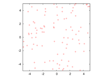
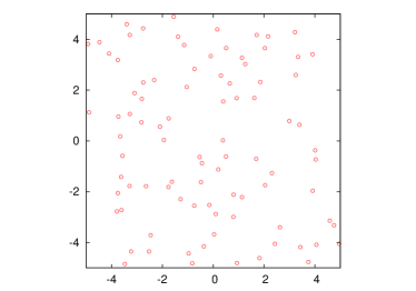
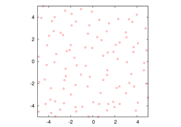
Figure 1: Samples of the Poisson ($\alpha\to 0$, left), $\alpha$-Ginibre ($\alpha=0.5$, center) and original Ginibre ($\alpha=1$, right) point processes with the same intensity. [19]

Remark 1

As seen in (9), the $\alpha$-Ginibre point process has the intensity $\pi^{-1}$ with respect to the Lebesgue measure; that is, for $C\in\mathcal{B}(\mathbb{C})$,

$$\mathsf{E}\Phi(C)=\int_{C}\rho_{\alpha}^{(1)}(z)\,\nu_{\alpha}(\mathrm{d}z)=\frac{\mu(C)}{\pi}.$$

However, we can consider the process with an arbitrary fixed intensity $\lambda\in(0,\infty)$ by scaling. The kernel and reference measure of the scaled $\alpha$-Ginibre point process with intensity $\lambda$ are respectively given by $K_{\alpha,\lambda}(z,w)=\mathrm{e}^{\pi\lambda z\overline{w}/\alpha}$ and $\nu_{\alpha,\lambda}(\mathrm{d}z)=\lambda\,\mathrm{e}^{-\pi\lambda|z|^{2}/\alpha}\,\mu(\mathrm{d}z)$. Or equivalently, the kernel $\widetilde{K}_{\alpha}^{(\lambda)}(z,w)=\lambda\,\mathrm{e}^{-\pi\lambda(|z|^{2}+|w|^{2})/(2\alpha)}\,\mathrm{e}^{\pi\lambda z\overline{w}/\alpha}$ with respect to the Lebesgue measure $\mu$ defines the same process.

We next see the nonzero eigenvalues and the corresponding eigenfunctions of the integral operator corresponding to the kernel $K_{\alpha}$. Let

$$\phi_{\alpha,i}(z)=\frac{z^{i-1}}{\sqrt{(i-1)!\,\alpha^{i}}},\quad i\in\mathbb{N}.$$ (11)

Then we can check that $\phi_{\alpha,i}$, $i\in\mathbb{N}$, are the orthonormal eigenfunctions of $K_{\alpha}$ corresponding to the eigenvalue $\alpha$ satisfying

$$\int_{\mathbb{C}}\phi_{\alpha,i(}z)\,\overline{\phi_{\alpha,j}(z)}\,\nu_{\alpha}(\mathrm{d}z)=\Biggl{\{}\vbox{\hbox{$1$\quad for $i=j$,} \hbox{$0$\quad for $i\neq j$.} }$$

Thus, Mercer’s spectral expansion ([35]) holds such that

$$K_{\alpha}(z,w)=\sum_{i=1}^{\infty}\alpha\,\phi_{\alpha,i}(z)\,\overline{\phi_{\alpha,i}(w)},\quad z,w\in\mathbb{C}.$$

Now, let $D_{r}$ denote the disk on $\mathbb{C}$ centered at the origin with radius $r$. Then $\phi_{\alpha,i}$, $i\in\mathbb{N}$, in (11) are also orthogonal eigenfunctions (but not normal now) of the restriction $K_{\alpha,D_{r}}$ of $K_{\alpha}$ on $D_{r}$ corresponding to the eigenvalues

$$\kappa_{\alpha,D_{r},i}=\alpha\,P(i,r^{2}/\alpha)=\alpha\,\frac{\gamma(i,r^{2}/\alpha)}{\Gamma(i)},\quad i\in\mathbb{N},$$ (12)

where $P(x,y)=\gamma(x,y)/\Gamma(x)$ denotes the regularized lower incomplete Gamma function with the lower incomplete Gamma function $\gamma(x,y)=\int_{0}^{y}t^{x-1}\,\mathrm{e}^{-t}\,\mathrm{d}t$ and the usual Gamma function $\Gamma(x)=\gamma(x,\infty)$. Let $\chi_{i}$, $i\in\mathbb{N}$, denote i.i.d. Bernoulli random variables with $\mathsf{P}(\chi_{i}=1)=\alpha$ and let $Y_{i}$, $i\in\mathbb{N}$, denote mutually independent random variables with $Y_{i}\sim\mathrm{Gam}(i,\alpha^{-1})$, where $\{\chi_{i}\}_{i\in\mathbb{N}}$ and $\{Y_{i}\}_{i\in\mathbb{N}}$ are also independent of each other. Then, since $\mathsf{P}(Y_{i}\leq r^{2})=P(i,r^{2}/\alpha)$, (5) and (12) imply

$$\Phi_{\alpha}(D_{r})\mathrel{\buildrel d\over{=}}\sum_{i\in\mathbb{N}}\chi_{i}\,\boldsymbol{1}_{\{Y_{i}\leq r^{2}\}}.$$

This observation is closely related to the following proposition, which is a generalization of Kostlan’s result [36] for the original Ginibre point process (see also [26, Theorem 4.7.1]).

Proposition 2

Let $X_{i}$, $i\in\mathbb{N}$, denote the points of the $\alpha$-Ginibre point process. Then, the set $\{|X_{i}|^{2}\}_{i\in\mathbb{N}}$ has the same distribution as $\check{\boldsymbol{Y}}=\{\check{Y}_{i}\}_{i\in\mathbb{N}}$, which is extracted from $\boldsymbol{Y}=\{Y_{i}\}_{i\in\mathbb{N}}$ such that $Y_{i}$, $i\in\mathbb{N}$, are mutually independent with $Y_{i}\sim\mathrm{Gam}(i,\alpha^{-1})$ and each $Y_{i}$ is added in $\check{\boldsymbol{Y}}$ with probability $\alpha$ and discarded with $1-\alpha$ independently of others.

Indeed, the $\alpha$-Ginibre point process $\Phi_{\alpha}$ is obtained from the original Ginibre process $\Phi=\Phi_{1}$ by retaining each point of $\Phi$ with probability $\alpha$ (removing it with $1-\alpha$) independently, and then applying the homothety of ratio $\sqrt{\alpha}$ to the retained points in order to maintain the original intensity of the Ginibre process $\Phi$ ([28]). Proposition 2 is useful for analyzing the cellular network models described in the preceding section since the path-loss function usually depends only on the distance from a BS. When we consider the scaled $\alpha$-Ginibre point process with intensity $\lambda\in(0,\infty)$ as in Remark 1, $\mathrm{Gam}(i,\alpha^{-1})$ in the above proposition is replaced by $\mathrm{Gam}(i,\pi\lambda/\alpha)$.

We can extend Proposition 2 to the process under the Palm distribution. Applying (6) to (7), the kernel $K_{\alpha}^{o}$ of the $\alpha$-Ginibre point process under the reduced Palm distribution given a point at the origin is

$$K_{\alpha}^{o}(z,w)=\mathrm{e}^{z\overline{w}/\alpha}-1,$$ (13)

with respect to the same reference measure $\nu_{\alpha}$ in (8). Thus, the first product density is given by

$$\rho_{\alpha}^{o(1)}(z)\,\nu_{\alpha}(\mathrm{d}z)=K_{\alpha}^{o}(z,z)\,\nu_{\alpha}(\mathrm{d}z)=\frac{1}{\pi}\,(1-\mathrm{e}^{-|z|^{2}/\alpha})\,\mu(\mathrm{d}z).$$

Note that the $\alpha$-Ginibre point process is no longer stationary under the Palm distribution and the intensity function is increasing according to the distance from the origin. The following Proposition is obtained by applying the kernel (13) to Theorem 4.7.1 of [26].

Proposition 3

Let $X^{o}_{i}$, $i\in\mathbb{N}$, denote the points of the $\alpha$-Ginibre point process under the reduced Palm distribution. Then, the set $\{|X^{o}_{i}|^{2}\}_{i\in\mathbb{N}}$ has the same distribution as $\check{\boldsymbol{Y}}^{o}=\{\check{Y}^{o}_{i}\}_{i\in\mathbb{N}}$, which is extracted from $\boldsymbol{Y}=\{Y^{o}_{i}\}_{i\in\mathbb{N}}$ such that $Y^{o}_{i}$, $i\in\mathbb{N}$, are mutually independent with $Y^{o}_{i}\sim\mathrm{Gam}(i+1,\alpha^{-1})$ and each $Y^{o}_{i}$ is added in $\check{\boldsymbol{Y}}^{o}$ with probability $\alpha$ and discarded with $1-\alpha$ independently of others.

Note that $\check{\boldsymbol{Y}}^{o}$ in Proposition 3 is obtained from $\check{\boldsymbol{Y}}$ in Proposition 2 by removing the exponentially distributed random variable $Y_{1}\sim\mathrm{Gam}(1,\alpha^{-1})$ if it is retained with probability $\alpha$ (see [28]).

4 Coverage analysis

In this section, we show some existing results on the coverage analysis of the cellular network models described in Section 2; that is, we give the numerically computable forms of the coverage probability for the two examples in Section 2. Here, the coverage probability is defined as the tail probability $\mathsf{P}(\mathsf{SINR}_{o}>\theta)$, $\theta>0$, of the SINR in (1), which represents the probability that the SINR for the typical user achieves a target threshold $\theta$.

4.1 Homogeneous single-antenna network

We here derive a numerically computable form of the coverage probability for the homogeneous single-antenna network model in Example 1, where the BSs are deployed according to the $\alpha$-Ginibre point process with intensity $\lambda\in(0,\infty)$. The corresponding result for the model with Poisson deployed BSs is also derived. The proof for the Poisson deployed BS model mainly follows [11] while that for the $\alpha$-Ginibre deployed BS model does [17, 19].

Theorem 1 ([11, 17, 19])

Consider the homogeneous single-antenna cellular network model in Example 1 with the path-loss function $\ell(r)=r^{-2\beta}$, $r>0$, for $\beta>1$, where $H_{i}\sim\mathrm{Exp}(1)$, $i\in\mathbb{N}$, (Rayleigh fading) and $G_{i}$, $i\in\mathbb{N}$, are i.i.d. When the point process $\Phi$ is the homogeneous Poisson point process with intensity $\lambda\in(0,\infty)$, the coverage probability for the typical user is given by

$$\mathsf{P}(\mathsf{SINR}_{o}^{(\text{PPP})}>\theta)=\int_{0}^{\infty}\exp\biggl{\{}-\frac{\theta\,w_{o}}{p}\,\biggl{(}\frac{t}{\pi\,\lambda}\biggr{)}^{\beta}-t\,\Bigl{(}1+\tau(\theta,\beta)\Bigr{)}\biggr{\}}\,\mathrm{d}t,$$ (14)

where

$$\tau(\theta,\beta)=\frac{\theta^{1/\beta}}{\beta}\int_{1/\theta}^{\infty}\bigl{(}1-\mathcal{L}_{G}(u^{-1})\bigr{)}\,u^{-1+1/\beta}\,\mathrm{d}u,$$ (15)

and $\mathcal{L}_{G}$ denotes the Laplace transform of $G_{i}$, $i\in\mathbb{N}$. On the other hand, when $\Phi$ is the $\alpha$-Ginibre point process with intensity $\lambda$,

$$\mathsf{P}(\mathsf{SINR}_{o}^{(\text{$\alpha$-GPP})}>\theta)=\alpha\int_{0}^{\infty}\exp\biggl{\{}-t-\frac{\theta\,w_{o}}{p}\,\biggl{(}\frac{\alpha\,t}{\pi\lambda}\biggr{)}^{\beta}\biggr{\}}\,M_{\alpha}(t,\theta,\beta)\,S_{\alpha}(t,\theta,\beta)\,\mathrm{d}t,$$ (16)

where

$$M_{\alpha}(t,\theta,\beta) =\prod_{i=0}^{\infty}\Bigl{[}1-\alpha+\alpha\,J_{i}(t,\theta,\beta)\Bigr{]},$$ (17)

$$S_{\alpha}(t,\theta,\beta) =\sum_{i=0}^{\infty}\frac{t^{i}}{i!}\,\Bigl{[}1-\alpha+\alpha\,J_{i}(t,\theta,\beta)\Bigr{]}^{-1},$$ (18)

with

$$J_{i}(t,\theta,\beta)=\frac{1}{i!}\int_{t}^{\infty}\mathrm{e}^{-u}\,u^{i}\,\mathcal{L}_{G}\biggl{(}\theta\,\biggl{(}\frac{t}{u}\biggr{)}^{\beta}\biggr{)}\,\mathrm{d}u.$$ (19)

For the proof of (14)–(15) for the Poisson deployed BS model, we use the probability generating functional for point processes.

Definition 1

Let $\Phi=\{X_{i}\}_{i\in\mathbb{N}}$ denote a point process on $\mathbb{R}^{d}$ with intensity measure $\Lambda$; that is, $\mathsf{E}\Phi(C)=\Lambda(C)$ for $C\in\mathcal{B}(\mathbb{R}^{d})$. For any measurable function $v$: $\mathbb{R}^{d}\to[0,1]$ such that $\int_{\mathbb{R}^{d}}\bigl{(}1-v(x)\bigr{)}\,\Lambda(\mathrm{d}x)<\infty$, the probability generating functional of the point process $\Phi$ is defined as

$$\mathcal{G}_{\Phi}(v)=\mathsf{E}\biggl{[}\prod_{i\in\mathbb{N}}v(X_{i})\biggr{]}.$$

Proposition 4 (e.g., [37, Sec. 9.4])

For the Poisson point process $\Phi$ on $\mathbb{R}^{d}$ with intensity measure $\Lambda$, its probability generating functional is given as

$$\mathcal{G}_{\Phi}^{(\text{PPP})}(v)=\exp\biggl{\{}-\int_{\mathbb{R}^{d}}\bigl{(}1-v(x)\bigr{)}\,\Lambda(\mathrm{d}x)\biggr{\}}.$$ (20)

Note that, if $\Phi$ is stationary with intensity $\lambda$, then $\Lambda(\mathrm{d}x)$ above is replaced by $\lambda\,\mathrm{d}x$.

Proof of Theorem 1:.

In the definition of the SINR in (1), each $H_{i}$ is independent of $\Phi=\{X_{i}\}_{i\in\mathbb{N}}$ and $\{G_{j}\}_{j\in\mathbb{N}\setminus\{i\}}$. Also, $\eta(o)$ is determined by $\Phi=\{X_{i}\}_{i\in\mathbb{N}}$. Thus, conditioning on $\Phi=\{X_{i}\}_{i\in\mathbb{N}}$ and $\{G_{j}\}_{j\in\mathbb{N}\setminus\{\eta(o)\}}$, and using $H_{i}\sim\mathrm{Exp}(1)$, $i\in\mathbb{N}$, we have

$$\mathsf{P}(\mathsf{SINR}_{o}>\theta)=\mathsf{P}\biggl{(}H_{\eta(o)}>\theta\,\frac{I_{o}(\eta(o))+w_{o}}{p\,\ell(|X_{\eta(o)}|)}\biggr{)}=\mathsf{E}\biggl{[}\exp\biggl{\{}-\theta\,\frac{I_{o}(\eta(o))+w_{o}}{p\,\ell(|X_{\eta(o)}|)}\biggr{\}}\biggr{]}.$$

Furthermore, the definition of the interference (2) and the Laplace transform of $G_{j}$, $j\in\mathbb{N}$, lead to

$$\mathsf{P}(\mathsf{SINR}_{o}>\theta)=\mathsf{E}\biggl{[}\exp\biggl{\{}-\frac{\theta\,w_{o}}{p\,\ell(|X_{\eta(o)}|)}\biggr{\}}\prod_{j\in\mathbb{N}\setminus\{\eta(o)\}}\!\mathcal{L}_{G}\biggl{(}\theta\,\frac{\ell(|X_{j}|)}{\ell(|X_{\eta(o)}|)}\biggr{)}\biggr{]},$$ (21)

which is the starting point for both the Poisson and $\alpha$-Ginibre deployed BS cellular network models.

We first show (14)–(15) for the Poisson deployed BS model. For the homogeneous Poisson point process $\Phi$ on $\mathbb{R}^{2}$ with intensity $\lambda$, the distribution for the distance to the nearest point from the origin is given by

$$\mathsf{P}(|X_{\eta(o)}|>r)=\mathsf{P}\bigl{(}\Phi(D_{r})=0\bigr{)}=\mathrm{e}^{-\lambda\pi r^{2}},$$ (22)

where $D_{r}$ denotes the disk centered at the origin with radius $r$. Given $|X_{\eta(o)}|=r$, other points of $\Phi$ also follow the Poisson point process on $\mathbb{R}^{2}\setminus D_{r}$, and thus applying the probability generating functional (20), we obtain

$$\mathsf{E}\biggl{[}\prod_{j\in\mathbb{N}}\mathcal{L}_{G}\biggl{(}\theta\,\frac{\ell(|X_{j}|)}{\ell(r)}\biggr{)}\biggm{|}X_{j}\in\mathbb{R}^{2}\!\setminus\!D_{r},\>j\in\mathbb{N}\biggr{]} =\exp\biggl{\{}-\lambda\int_{|x|>r}\biggl{[}1-\mathcal{L}_{G}\biggl{(}\theta\,\frac{\ell(|x|)}{\ell(r)}\biggr{)}\biggr{]}\,\mathrm{d}x\biggr{\}}$$

$$=\exp\biggl{\{}-2\pi\lambda\int_{r}^{\infty}\biggl{[}1-\mathcal{L}_{G}\biggl{(}\theta\,\frac{\ell(s)}{\ell(r)}\biggr{)}\biggr{]}\,s\,\mathrm{d}s\biggr{\}}.$$ (23)

Hence, applying (22), (4.1) and $\ell(r)=r^{-2\beta}$ to (21) yields (14)–(15) after some manipulations.

On the other hand, for the $\alpha$-Ginibre deployed BS model, we use $\boldsymbol{Y}=\{Y_{i}\}_{i\in\mathbb{N}}$ in Proposition 2 such that $Y_{i}$, $i\in\mathbb{N}$, are mutually independent and each $Y_{i}$ is retained with probability $\alpha$ independently of others. Thus, dividing the cases in each of which the point corresponding to $Y_{i}$ is retained and associated with the typical user, (21) with $\ell(r)=r^{-2\beta}$ reduces to

$$\mathsf{P}(\mathsf{SINR}_{o}^{(\text{$\alpha$-GPP})}>\theta) =\alpha\sum_{i\in\mathbb{N}}\mathsf{E}\biggl{[}\exp\biggl{\{}-\frac{\theta\,w_{o}}{p}\,{Y_{i}}^{\beta}\biggr{\}}\prod_{j\in\mathbb{N}\setminus\{i\}}\biggl{\{}1-\alpha+\alpha\,\mathcal{L}_{G}\biggl{(}\theta\,\biggl{(}\frac{Y_{i}}{Y_{j}}\biggr{)}^{\beta}\biggr{)}\,\boldsymbol{1}_{\{Y_{j}\geq Y_{i}\}}\biggr{\}}\biggr{]}.$$

Finally, applying $Y_{i}\sim\mathrm{Gam}(i,\pi\lambda/\alpha)$, $i\in\mathbb{N}$ yields (16)–(19) after some manipulations.  ∎

Figure 2 shows the comparison result of the coverage probability with different values of $\alpha$. Each plot indicates the coverage probability for a given value of $\theta$ in the case of $w_{o}=0$ (noise-free) and $\beta=2$ (i.e., $\ell(r)=r^{-4}$). It seems that the coverage probability is increasing in $\alpha$. However, a numerical result in [18] shows that the coverage probability is not always monotone in $\alpha$ as $\theta\to\infty$.

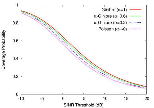
Figure 2: Comparison of coverage probability in terms of $\alpha$ in the single tier model ($\ell(r)=r^{-4}$, no noise). [19]

4.2 Two-tier Ginibre-Poisson overlaid network

In this subsection, we consider the case of $K=2$ in Example 2, where the BSs of tier $1$ are deployed according to the $\alpha$-Ginibre point process $\Phi_{1}$ with intensity $\lambda_{1}$ while the BSs of tier $2$ follow the homogeneous Poisson point process $\Phi_{2}$ with intensity $\lambda_{2}$. This represents that, in heterogeneous multi-tier cellular networks, the macro BSs are deployed rather systematically while the femto BSs are located in an opportunistic manner. We assume that the two point processes $\Phi_{1}$ and $\Phi_{2}$ are independent of each other. In the coverage of users, the target thresholds can differ for the two tiers; that is, the SINR should be larger than $\theta_{k}$ when a user is served by a BS of tier $k$ for $k=1$, $2$.

For the ease of understanding, we impose some extent of simplifying setting (see [23] for a general setting). First, we ignore the noise power and set $w_{o}=0$, in this case, the SINR in (1) is called the signal-to-interference ratio (SIR). Furthermore, we only consider the case where the number of users served at each BS is equal to the number of antennas; that is, $m_{k}=\psi_{k}$ for $k=1$, $2$. This case reduces to the single-input single-output (SISO) transmission when $m_{k}=\psi_{k}=1$ while this is called the full form of space-division multiple access (full SDMA) transmission when $m_{k}=\psi_{k}>1$. In this setting, $H_{i}\sim\mathrm{Exp}(1)$, $i\in\mathbb{N}$, since $\delta_{k}=1$ for each $k\in\mathcal{K}$, and they are mutually independent.

Theorem 2

Consider the two-tier multi-antenna cellular network model in Example 2 with $K=2$, $\ell_{1}(r)=r^{-2\beta_{1}}$ and $\ell_{2}(r)=r^{-2\beta_{2}}$. Then, under the setting described above, the coverage probability for the typical user is given by

$$\mathsf{P}(\mathsf{SIR}_{o}^{(\mathrm{MIMO})}>\theta_{\xi_{\eta(o)}}) =\alpha\int_{0}^{\infty}M_{\alpha}(t,\theta_{1},\beta_{1})\,S_{\alpha}(t,\theta_{1},\beta_{1})$$ (24a)

$$\qquad\mbox{}\times\exp\biggl{\{}-t-C_{\alpha}^{(1,2)}(t)\,\bigl{(}1+\tau_{1,2}(\theta_{1},\beta_{2}\bigr{)}\biggr{\}}\,\mathrm{d}t$$ (24b)

$$\quad\mbox{}+\int_{0}^{\infty}M_{\alpha}^{(2,1)}(t,\theta_{2},\beta_{1},\beta_{2})$$ (24c)

$$\quad\qquad\mbox{}\times\exp\Bigl{\{}-t\,\bigl{(}1+\tau(\theta_{2},\beta_{2})\bigr{)}\Bigr{\}}\ \mathrm{d}t$$ (24d)

where $M_{\alpha}(t,\theta,\beta)$ and $S_{\alpha}(t,\theta,\beta)$ are the same as in (17) and (18) respectively with $\mathcal{L}_{G}(s)=\mathcal{L}_{G,1}(s)=(1+s)^{-\psi_{1}}$ in $J_{i}$ in (19). Moreover,

$$C_{\alpha}^{(1,2)}(t) =\pi\lambda_{2}\,\biggl{(}\frac{b_{2}p_{2}}{b_{1}p_{1}}\biggr{)}^{1/\beta_{2}}\,\biggl{(}\frac{\alpha t}{\pi\lambda_{1}}\biggr{)}^{\beta_{1}/\beta_{2}},$$

$$\tau_{1,2}(\theta,\beta) =\frac{\theta^{1/\beta}}{\beta}\int_{1/\theta}^{\infty}\biggl{[}1-\biggl{(}\frac{u}{u+b_{1}/b_{2}}\biggr{)}^{\psi_{2}}\biggr{]}\,u^{-1+1/\beta}\,\mathrm{d}u,$$

and

$$M_{\alpha}^{(2,1)}(t,\theta,\beta_{1},\beta_{2})=\prod_{i=0}^{\infty}\Bigl{[}1-\alpha+\alpha\,J_{\alpha,i}^{(2,1)}(t,\theta,\beta_{1},\beta_{2})\Bigr{]},$$

where

$$J_{\alpha,i}^{(2,1)}(t,\theta,\beta_{1},\beta_{2}) =\frac{1}{i!}\int_{C_{\alpha}^{(2,1)}(t)}^{\infty}\mathrm{e}^{-u}\,u^{i}\,\biggl{[}1+\theta\,\frac{p_{1}}{p_{2}}\,\frac{(t/\pi\lambda_{2})^{\beta_{2}}}{(\alpha u/\pi\lambda_{1})^{\beta_{1}}}\biggr{]}^{-\psi_{1}}\mathrm{d}u,$$

with

$$C_{\alpha}^{(2,1)}(t)=\frac{\pi\lambda_{1}}{\alpha}\,\biggl{(}\frac{b_{1}p_{1}}{b_{2}p_{2}}\biggr{)}^{1/\beta_{1}}\,\biggl{(}\frac{t}{\pi\lambda_{2}}\biggr{)}^{\beta_{2}/\beta_{1}}.$$

$\tau(\theta,\beta)$ is also the same as in (15) with $\mathcal{L}_{G}(u^{-1})=\mathcal{L}_{G,2}(u^{-1})=\bigl{[}u/(u+1)\bigr{]}^{\psi_{2}}$.

The proof is placed in the appendix and we here make a short remark on Theorem 2. The formula of the coverage probability in the theorem consists of two parts (24a)–(24b) and (24c)–(24d). The first part corresponds to that the typical user is served by a BS of tier $1$, so that the term in (24a) is given as the same form as in (16). The term in (24b) corresponds to the cumulative interference from all the BSs of tier $2$, which can be seen similar to the second term in the exponential in (14). The second part (24c)–(24d) corresponds to that the typical user is served by a BS of tier $2$, so that the term in (24d) has the same form as the second term in the exponential in (14). The term in (24c) corresponds to the cumulative interference from all the BSs of tier $1$, so that $M_{\alpha}^{(2,1)}$ has a similar form to $M_{\alpha}$ in (17) (the term corresponding to $S_{\alpha}$ does not appear in this case).

5 Conclusion

In this tutorial, we have introduced the $\alpha$-Ginibre point process as the model of BS deployments in cellular networks. First, we have reviewed the definition and some useful properties of this process, and then we have seen the two existing results on the coverage analysis of cellular network models, where the BSs are deployed according to the $\alpha$-Ginibre point processes. The authors now hope that the readers will use the ($\alpha$-)Ginibre point process and challenge themselves to various problems arising in future cellular networks.

Finally, when we use the Ginibre and other determinantal point processes as the models of BS deployments, we might face to a computation problem. Although the obtained formulas are indeed numerically computable, as seen in (16)–(19) and (24a)–(24d), they include infinite sums and infinite products, which may lead to the time-consuming computation. One direction to avoid this problem could be some kinds of asymptotics and/or approximation (see, e.g., [18, 21, 38, 39, 40] for this direction).

Appendix A Proof of Theorem 2

We divide the coverage probability into two cases according to the tier of the BS associated with the typical user;

$$\mathsf{P}\bigl{(}\mathsf{SIR}_{o}^{(\mathrm{MIMO})}>\theta_{\xi_{\eta(o)}}\bigr{)} =\mathsf{P}\bigl{(}\mathsf{SIR}_{o}^{(\mathrm{MIMO})}>\theta_{1},\>\xi_{\eta(o)}=1\bigr{)}+\mathsf{P}\bigl{(}\mathsf{SIR}_{o}^{(\mathrm{MIMO})}>\theta_{2},\>\xi_{\eta(o)}=2\bigr{)},$$ (25)

and consider the two terms separately.

Case of $\xi_{\eta(o)}=1$:

Let $\mathbb{N}_{1}$ and $\mathbb{N}_{2}$ denote the random partition of $\mathbb{N}$ such that $\mathbb{N}_{k}=\{i\in\mathbb{N}:\xi_{i}=k\}$ for $k=1$, $2$. Then, the interference (2) for $i\in\mathbb{N}_{1}$ is written as

$$I_{o}(i)=\sum_{j\in\mathbb{N}_{1}\setminus\{i\}}p_{1}\,G_{j}\,\ell_{1}(|X_{j}|)+\sum_{j\in\mathbb{N}_{2}}p_{2}\,G_{j}\,\ell_{2}(|X_{j}|).$$

Applying this to the first term on the right-hand side of (25) yields

$$\mathsf{P}\bigl{(}\mathsf{SIR}_{o}^{(\mathrm{MIMO})}>\theta_{1},\>\xi_{\eta(o)}=1\bigr{)}$$

$$=\mathsf{E}\Biggl{[}\exp\biggl{\{}-\theta_{1}\,\frac{I_{o}(\eta(o))}{p_{1}\,\ell_{1}(|X_{\eta(o)}|)}\biggr{\}}\,\boldsymbol{1}_{\{\xi_{\eta(o)}=1\}}\Biggr{]}$$

$$=\mathsf{E}\Biggl{[}\prod_{j\in\mathbb{N}_{1}\setminus\{\eta(o)\}}\mathcal{L}_{G,1}\Biggl{(}\theta_{1}\,\biggl{(}\frac{|X_{\eta(o)}|}{|X_{j}|}\biggr{)}^{2\beta_{1}}\Biggr{)}\prod_{j\in\mathbb{N}_{2}}\mathcal{L}_{G,2}\Biggl{(}\theta_{1}\frac{p_{2}}{p_{1}}\frac{|X_{\eta(o)}|^{2\beta_{1}}}{|X_{j}|^{2\beta_{2}}}\Biggr{)}\,\boldsymbol{1}_{\{\xi_{\eta(o)}=1\}}\Biggr{]},$$ (26)

where $\ell_{1}(r)=r^{-2\beta_{1}}$ and $\ell_{2}(r)=r^{-2\beta_{2}}$ are also used. Note here that $\{\eta(o)=i\}$ with $i\in\mathbb{N}_{1}$ implies $\{|X_{j}|\geq|X_{i}|\}$ for $j\in\mathbb{N}_{1}$ while for $j\in\mathbb{N}_{2}$,

$$\{b_{1}p_{1}|X_{i}|^{-2\beta_{1}}\geq b_{2}p_{2}|X_{j}|^{-2\beta_{2}}\}=\{|X_{j}|\geq R_{1,2}(|X_{i}|)\},$$

with $R_{1,2}(r)=(b_{2}p_{2}/(b_{1}p_{1}))^{1/(2\beta_{2})}r^{\beta_{1}/\beta_{2}}$. Thus, using $\boldsymbol{Y}=\{Y_{i}\}_{i\in\mathbb{N}}$ in Proposition 2, (A) further reduces to

$$\mathsf{P}\bigl{(}\mathsf{SIR}_{o}^{(\mathrm{MIMO})}>\theta_{1},\>\xi_{\eta(o)}=1\bigr{)} =\alpha\sum_{i\in\mathbb{N}}\mathsf{E}\Biggl{[}\prod_{j\in\mathbb{N}\setminus\{i\}}\Biggl{\{}1-\alpha+\alpha\,\mathcal{L}_{G,1}\Biggl{(}\theta_{1}\,\Biggl{(}\frac{Y_{i}}{Y_{j}}\Biggr{)}^{\beta_{1}}\Biggr{)}\,\boldsymbol{1}_{\{Y_{j}>Y_{i}\}}\Biggr{\}}$$

$$\qquad\mbox{}\times\prod_{j\in\mathbb{N}}\mathcal{L}_{G,2}\Biggl{(}\theta_{1}\frac{p_{2}}{p_{1}}\frac{{Y_{i}}^{\beta_{1}}}{|X_{2,j}|^{2\beta_{2}}}\Biggr{)}\,\boldsymbol{1}_{\{|X_{2,j}|\geq R_{1,2}({Y_{i}}^{1/2})\}}\Biggr{]},$$ (27)

where $\{X_{2,j}\}_{j\in\mathbb{N}}$ follows the homogeneous Poisson point process with intensity $\lambda_{2}$. Conditioning on $Y_{i}$ and applying the generating functional (20) to the second infinite product on the right-hand side of (A), we have

$$\mathsf{E}\Biggl{[}\prod_{j\in\mathbb{N}}\mathcal{L}_{G,2}\Biggl{(}\theta_{1}\frac{p_{2}}{p_{1}}\frac{{Y_{i}}^{\beta_{1}}}{|X_{2,j}|^{2\beta_{2}}}\Biggr{)}\,\boldsymbol{1}_{\{|X_{2,j}|\geq R_{1,2}({Y_{i}}^{1/2})\}}\Biggm{|}Y_{i}\Biggr{]}$$

$$=\exp\Biggl{\{}-\lambda_{2}\!\!\int_{\mathbb{R}^{2}}\Biggl{[}1\!-\!\mathcal{L}_{G,2}\Biggl{(}\theta_{1}\frac{p_{2}}{p_{1}}\frac{{Y_{i}}^{\beta_{1}}}{|x|^{2\beta_{2}}}\Biggr{)}\boldsymbol{1}_{\{|x|\geq R_{1,2}({Y_{i}}^{1/2})\}}\Biggr{]}\mathrm{d}x\Biggr{\}}$$

$$=\exp\Biggl{\{}-\pi\lambda_{2}\biggl{(}\frac{b_{2}p_{2}}{b_{1}p_{1}}\biggr{)}^{1/\beta_{2}}{Y_{i}}^{\beta_{1}/\beta_{2}}\,\Bigl{(}1+\tau_{1,2}(\theta_{1},\beta_{2})\Bigr{)}\Biggr{\}},$$ (28)

where

$$\tau_{1,2}(\theta,\beta)=\frac{\theta^{1/\beta}}{\beta}\int_{1/\theta}^{\infty}\biggl{[}1-\biggl{(}\frac{u}{u+b_{1}/b_{2}}\biggr{)}^{\psi_{2}}\biggr{]}\,u^{-1+1/\beta}\,\mathrm{d}u.$$

Hence, substituting (A) to (A) and applying $Y_{i}\sim\mathrm{Gam}(i,\pi\lambda_{1}/\alpha)$, $i\in\mathbb{N}$, we obtain (24a)–(24b) after some manipulations.

Case of $\xi_{\eta(o)}=2$:

Similar to the above, the second term on the right-hand side of (25) is given as

$$\mathsf{P}\bigl{(}\mathsf{SIR}_{o}^{(\mathrm{MIMO})}>\theta_{2},\>\xi_{\eta(o)}=2\bigr{)}$$

$$=\mathsf{E}\Biggl{[}\prod_{j\in\mathbb{N}_{1}}\mathcal{L}_{G,1}\Biggl{(}\theta_{2}\,\frac{p_{1}}{p_{2}}\frac{|X_{\eta(o)}|^{2\beta_{2}}}{|X_{j}|^{2\beta_{1}}}\Biggr{)}\prod_{j\in\mathbb{N}_{2}\setminus\{\eta(o)\}}\mathcal{L}_{G,2}\Biggl{(}\theta_{2}\,\biggl{(}\frac{|X_{\eta(o)}|}{|X_{j}|}\biggr{)}^{2\beta_{2}}\Biggr{)}\,\boldsymbol{1}_{\{\xi_{\eta(o)}=2\}}\Biggr{]}.$$ (29)

Now, $\{\eta(o)=i\}$ with $i\in\mathbb{N}_{2}$ implies that

$$\{b_{2}p_{2}|X_{i}|^{-2\beta_{2}}\geq b_{1}p_{1}|X_{j}|^{-2\beta_{1}}\}=\{|X_{j}|\geq R_{2,1}(|X_{i}|)\},$$

with $R_{2,1}(r)=(b_{1}p_{1}/(b_{2}p_{2}))^{1/(2\beta_{1})}r^{\beta_{2}/\beta_{1}}$ for $i\in\mathbb{N}_{1}$ while $\{|X_{j}|\geq|X_{i}|\}$ for $j\in\mathbb{N}_{2}$. Therefore, using the distribution of $|X_{\eta(o)}|$ in (22) and also $\boldsymbol{Y}=\{Y_{i}\}_{i\in\mathbb{N}}$ in Proposition 2, (A) reduces to

$$\mathsf{P}\bigl{(}\mathsf{SIR}_{o}^{(\mathrm{MIMO})}>\theta_{2},\>\xi_{\eta(o)}=2\bigr{)} =\int_{0}^{\infty}2\pi\lambda_{2}\,r\,\mathrm{e}^{-\lambda_{2}\pi r^{2}}\mathsf{E}\Biggl{[}\prod_{j\in\mathbb{N}}\Biggl{\{}1-\alpha+\alpha\,\mathcal{L}_{G,1}\Biggl{(}\theta_{2}\frac{p_{1}}{p_{2}}\frac{r^{2\beta_{2}}}{{Y_{j}}^{\beta_{1}}}\Biggr{)}\,\boldsymbol{1}_{\{Y_{j}\geq R_{2,1}(r)^{2}\}}\Biggr{\}}\Biggr{]}$$

$$\qquad\mbox{}\times\mathsf{E}\Biggl{[}\prod_{j\in\mathbb{N}}\mathcal{L}_{G,2}\Biggl{(}\theta_{2}\biggl{(}\frac{r}{|X_{2,j}|}\biggr{)}^{2\beta_{2}}\Biggr{)}\Biggm{|}|X_{2,j}|\geq r,j\in\mathbb{N}\Biggr{]}\,\mathrm{d}r,$$ (30)

where by applying (20), the second expectation in the integrand of (A) is equal to

$$\mathsf{E}\Biggl{[}\prod_{j\in\mathbb{N}}\mathcal{L}_{G,2}\Biggl{(}\theta_{2}\biggl{(}\frac{r}{|X_{2,j}|}\biggr{)}^{2\beta_{2}}\Biggr{)}\Biggm{|}|X_{2,j}|\geq r,j\in\mathbb{N}\Biggr{]} =\exp\Biggl{\{}-2\pi\lambda_{2}\int_{r}^{\infty}\Biggl{[}1-\mathcal{L}_{G,2}\Biggl{(}\theta_{2}\biggl{(}\frac{r}{s}\biggr{)}^{2\beta_{2}}\Biggr{)}\Biggr{]}\,s\,\mathrm{d}s\Biggr{\}}.$$

Hence, substituting this to (A) and applying $Y_{i}\sim\mathrm{Gam}(i,\pi\lambda_{1}/\alpha)$, $i\in\mathbb{N}$, we obtain (24c)–(24d) after some manipulations.  ∎

References

• [1] J. G. Andrews, R. K. Ganti, M. Haenggi, N. Jindal, and S. Weber, “A primer on spatial modeling and analysis in wireless networks,” IEEE Commun. Magazine, vol. 48, pp. 156–163, 2010.
• [2] M. Haenggi, J. G. Andrews, F. Baccelli, O. Dousse, and M. Franceschetti, “Stochastic geometry and random graphs for the analysis and design of wireless networks,” IEEE J. Select. Areas Commun., vol. 27, pp. 1029–1046, 2009.
• [3] H. ElSawy, E. Hossain, and M. Haenggi, “Stochastic geometry for modeling, analysis, and design of multi-tier and cognitive cellular wireless networks: A survey,” IEEE Commun. Surveys Tutorials, vol. 15, pp. 996–1019, 2013.
• [4] H. ElSawy, A. Sultan-Salem, M. S. Alouini, and M. Z. Win, “Modeling and analysis of cellular networks using stochastic geometry: A tutorial,” arXiv: 1604.03689 [cs.IT], 2016.
• [5] F. Baccelli and B. Błaszczyszyn, “Stochastic geometry and wireless networks, Volume I: Theory,” Found. Trends Networking, vol. 3, pp. 249–449, 2009.
• [6] F. Baccelli and B. Błaszczyszyn, “Stochastic geometry and wireless networks, Volume II: Applications,” Found. Trends Networking, vol. 4, pp. 1–312, 2009.
• [7] M. Haenggi, Stochastic Geometry for Wireless networks, Cambridge Univ. Press, 2013.
• [8] S. Mukherjee, Analytical Modeling of Heterogeneous Cellular Networks: Geometry, Coverage, and Capacity, Cambridge Univ. Press, 2014.
• [9] H. ElSawy and E. Hossain, “Two-tier HetNets with cognitive femto-cells: Downlink performance modeling and analysis in a multichannel environment,” IEEE Trans. Mobile Comput., vol. 13, pp. 649–663, 2014.
• [10] M. Wildemeersch, M.K. T. Quek, A. Rabbachin, and C. Slump, “Successive interference cancellation in heterogeneous networks,” IEEE Trans. Commun., vol. 62, pp. 4440–4453, 2014.
• [11] J. G. Andrews, F. Baccelli, and R. K. Ganti, “A tractable approach to coverage and rate in cellular networks,” IEEE Trans. Commun., vol. 59, pp. 3122–3134, 2011.
• [12] H. S. Dhillon, R. K. Ganti, F. Baccelli, and J. G. Andrews, “Modeling and analysis of $K$-tier downlink heterogeneous cellular networks,” IEEE J. Select. Areas Commun., vol. 30, pp. 550–560, 2012.
• [13] H. S. Jo, Y. J. Sang, P. Xia, and J. G. Andrews, “Heterogeneous cellular networks with flexible cell association: A comprehensive downlink SINR analysis,” IEEE Trans. Wireless Commun., vol. 11, pp. 3484–3495, 2012.
• [14] S. Mukherjee, “Downlink SINR distribution in a heterogeneous cellular wireless network,” IEEE J. Select. Areas Commun., vol. 30, pp. 575–585, 2012.
• [15] M. D. Renzo, A. Guidotti, and G. E. Corazza, “Average rate of downlink heterogeneous cellular networks over generalized fading channels: A stochastic geometry approach,” IEEE Trans. Commun., vol. 61, pp. 3050–3071, 2013.
• [16] A. Guo and M. Haenggi, “Spatial stochastic models and metrics for the structure of base stations in cellular networks,” IEEE Trans. Wireless Commun., vol. 12, pp. 5800–5812, 2013.
• [17] N. Miyoshi and T. Shirai, “A cellular network model with Ginibre configured base stations,” Adv. Appl. Probab., vol. 46, pp. 832–845, 2014.
• [18] N. Miyoshi and T. Shirai, “Cellular networks with $\alpha$-Ginibre configurated base stations,” The Impact of Applications on Mathematics: Proc. Forum Math. Industry 2013, pp. 211–226, Springer, 2014.
• [19] I. Nakata and N. Miyoshi, “Spatial stochastic models for analysis of heterogeneous cellular networks with repulsively deployed base stations,” Perform. Eval., vol. 78, pp. 7–17, 2014.
• [20] T. Kobayashi and N. Miyoshi, “Uplink cellular network models with Ginibre deployed base stations,” ITC-26, 2014.
• [21] H. Nagamatsu, N. Miyoshi, and T. Shirai, “Padé approximation for coverage probability in cellular networks,” WiOpt 2014, pp. 693–700, 2014.
• [22] N. Miyoshi and T. Shirai, “Downlink coverage probability in a cellular network with Ginibre deployed base stations and Nakagami-$m$ fading channels,” WiOpt 2015, pp. 483–489, 2015.
• [23] T. Kobayashi and N. Miyoshi, “Downlink coverage probability in Ginibre-Poisson overlaid MIMO cellular networks,” WiOpt 2016, pp. 369–376, 2016.
• [24] A. Soshnikov, “Determinantal random point fields,” Russian Math. Surveys, vol. 55, pp. 923–975, 2000.
• [25] T. Shirai and Y. Takahashi, “Random point fields associated with certain Fredholm determinants I: Fermion, Poisson and Boson processes,” J. Funct. Analysis, vol. 205, pp. 414–463, 2003.
• [26] J. B. Hough, M. Krishnapur, Y. Peres, and B. Virág, Zeros of Gaussian Analytic Functions and Determinantal Point Processes, American Math. Soc., 2009.
• [27] F. Lavancier, J. Møller, and E. Rubak, “Determinantal point process models and statistical inference,” J. Royal Stat. Soc.: Ser. B, vol. 77, pp. 853–877, 2015.
• [28] A. Goldman, “The Palm measure and the Voronoi tessellation for the Ginibre process,” Annals Appl. Probab., vol. 20, pp. 90–128, 2010.
• [29] N. Deng, W. Zhou, and M. Haenggi, “The Ginibre point process as a model for wireless networks with repulsion,” IEEE Trans. Wireless Commun., vol. 14, pp. 107–121, 2015.
• [30] J. S. Gomez, A. Vasseur, A. Vergne, L. Decreusefond, and W. Chen, “A case study on regularity in cellular network deployment,” IEEE Wireless Commun. Letters, vol. 4, pp. 421–424, 2015.
• [31] Y. Li, F. Baccelli, H. S. Dhillon, and J. G. Andrews, “Statistical modeling and probabilistic analysis of cellular networks with determinantal point processes,” IEEE Trans. Commun., vol. 63, pp. 3405–3422, 2015.
• [32] H. Huang, C. B. Papadias, and S. Venkatesan, MIMO Communication for Cellular Networks, Springer, 2012.
• [33] H. S. Dhillon, M. Kountouris, and J. G. Andrews, “Downlink MIMO HetNets: Modeling, ordering results and performance analysis,” IEEE Trans. Wireless Commun., vol. 12, pp. 5208–5222, 2013.
• [34] A. K. Gupta, H. S. Dhillon, S. Vishwanath, and J. G. Andrews, “Downlink coverage probability in MIMO HetNets with flexible cell selection,” IEEE GLOBECOM 2014, pp. 1534–1539, 2014.
• [35] J. Mercer, “Functions of positive and negative type, and their connection with the theory of integral equations,” Philos. Trans. Royal Soc. London: Ser. A, vol. 209, pp. 415–446, 1909.
• [36] E. Kostlan, “On the spectra of Gaussian matrices,” Linear Algebra Appl., vol. 162–164, pp. 385–388, 1992.
• [37] D. J. Daley and D. Vere-Jones, An Introduction to the Theory of Point Processes, Volume II: General Theory and Structure, Second ed., Springer, 2008.
• [38] R. K. Ganti and M. Haenggi, “Asymptotics and approximation of the SIR distribution in general cellular networks,” IEEE Trans. Wireless Commun., vol. 15, pp. 2130–2143, 2016.
• [39] H. Wei, N. Deng, W. Zhou, and M. Haenggi, “Approximate SIR analysis in general heterogeneous cellular networks,” IEEE Trans. Commun., vol. 64, pp. 1259–1273, 2016.
• [40] N. Miyoshi and T. Shirai, “A sufficient condition for tail asymptotics of SIR distribution in downlink cellular networks,” WiOpt 2016, pp.454–460, 2016.