Arbitrage-Free Combinatorial Market Making via Integer Programming

Abstract

We present a new combinatorial market maker that operates arbitrage-free combinatorial prediction markets specified by integer programs. Although the problem of arbitrage-free pricing, while maintaining a bound on the subsidy provided by the market maker, is #P-hard in the worst case, we posit that the typical case might be amenable to modern integer programming (IP) solvers. At the crux of our method is the Frank-Wolfe (conditional gradient) algorithm which is used to implement a Bregman projection aligned with the market maker’s cost function, using an IP solver as an oracle. We demonstrate the tractability and improved accuracy of our approach on real-world prediction market data from combinatorial bets placed on the 2010 NCAA Men’s Division I Basketball Tournament, where the outcome space is of size $2^{63}$. To our knowledge, this is the first implementation and empirical evaluation of an arbitrage-free combinatorial prediction market on this scale.

2940716.2940767

Author addresses: C. Kroer, Computer Science Dept, CMU; ckroer@cs.cmu.edu; M. Dudík and S. Lahaie, Microsoft Research; {mdudik,slahaie}@microsoft.com; S. Balakrishnan, Dept of Statistics, CMU; siva@stat.cmu.edu. This work was done while C. Kroer and S. Balakrishnan were at Microsoft Research.

1 Introduction

Prediction markets have been successfully used to elicit and aggregate forecasts in a variety of domains, including business [21, 6], politics [4], and entertainment [20]. In a prediction market, traders buy and sell securities with values that depend on some unknown future outcome. For instance, a play-money prediction market that Yahoo! ran for the 2010 NCAA Men’s Division I Basketball Tournament included a security that paid out 1 point if the team from Duke were to win the championship and 0 points otherwise. Thus, when the price of the security was 0.15, traders who believed that Duke’s probability of winning was larger than 0.15 were incentivized to buy shares of the security, and those that believed it was lower were incentivized to sell. The market price can be interpreted as an aggregate belief and used as a forecast.

We study prediction markets implemented by a centralized algorithm called a cost-based market maker [10, 2]. All shares are bought from and sold to the market maker, rather than between traders, and the market maker uses a convex potential function to determine current security prices. Compared with an exchange, which matches buyers and sellers, a market-maker mechanism is particularly desirable in combinatorial markets, which offer securities on interrelated propositions. For instance, the NCAA 2010 market included securities on events “Duke wins more games than Cornell” and “a team from the Big East conference wins the championship” as well as many others. Because of the large number of securities in combinatorial markets, there may be no sellers interested in trading with a given buyer, a problem known as low liquidity. In contrast, a market maker is always available to trade, thus providing liquidity and allowing incorporation of information in the market.

Designers of cost-based markets aim to meet several desirable properties, including boundedness of loss suffered by the market maker and absence of arbitrage, that is, risk-free profitable trades. Bounded loss is a necessity for money markets, otherwise the market operator risks bankruptcy. Lack of arbitrage is also highly desirable. First, we would like to attract traders that provide information rather than computation. Second, arbitrage-free markets produce more accurate forecasts. While Abernethy et al. [2] provide a complete theoretical characterization of cost-based markets with bounded loss and no arbitrage, pricing in such markets is NP-hard or #P-hard for even the simplest combinatorial settings [7]. Previous solutions restrict the betting language to allow polynomial time algorithms [e.g., 8, 9, 22] or devise approximations [12].

In this paper we move beyond the hardness barrier. We hypothesize that while the pricing may be difficult in the worst case, a typical case is amenable to modern integer programming solvers. Guided by this hypothesis, we propose a fully general, bounded-loss, arbitrage-free market maker based on integer programming (IP) methods. Our market maker is guaranteed to maintain bounded loss, and attempts to remove arbitrage by making calls to the IP solver.

Our mechanism begins with any bounded-loss cost function and adds two ingredients. First, we use an integer program to specify the set of valid payoff vectors, each of which enumerates the security payoffs in a single outcome. Arbitrage-free prices are exactly the convex combinations of valid payoff vectors. Second, as we run the cost-based market, we periodically remove arbitrage by projecting the market state onto the set of arbitrage-free prices, using the IP solver as an oracle within the projection algorithm. The integer program for payoff vectors is typically compact in size and easy to specify based on security definitions. For instance, when securities correspond to logical propositions, outcomes correspond to truth-assignment of literals, and each valid payoff vector enumerates 0 for false and 1 for true propositions in a given outcome. Conjunctions and disjunctions are easily expressed within an IP, so we have a compact representation for all problems in NP. To implement projection, we use the Frank-Wolfe algorithm [14, 17], also known as the conditional gradient algorithm, which is well-suited to our setting because it only accesses the target set (in our case, the set of valid payoff vectors) through the operation of linear optimization, which can be handled by an IP solver. The projection that we consider is the Bregman projection, which generalizes the Euclidean projection to arbitrary convex potentials.

There are two specific issues in applying the Frank-Wolfe (FW) algorithm within cost-based markets. First, while all iterates of the FW algorithm are within the convex hull of valid payoff vectors, and therefore arbitrage-free, we need to ensure that bounded loss is maintained. In Sec. 4.2, we show how to achieve this by a suitable modification of the stopping condition of FW. The second, seemingly more serious concern, is that the projection problems that arise for common cost functions, such as Hanson’s 2003, 2007 logarithmic market scoring rule (LMSR), exhibit derivatives that go to infinity at the border of the set of arbitrage-free prices, which violates the assumptions of the FW algorithm. Fortunately, we can adapt a recently developed variant of FW [18], designed for the case when the derivative might grow to infinity, but its growth is suitably controlled, which is the case for LMSR.

Our approach, which we call the Frank-Wolfe market maker (FWMM), is related to DudikLaPe12’s [2012] linearly-constrained market maker (LCMM), which also alternates trades and (partial) arbitrage removal. While FWMM uses linear constraints in the IP to define valid payoff vectors, the arbitrage removal in LCMM is driven by a set of linear constraints on the arbitrage-free prices (i.e., the convex hull of valid payoff vectors). The IP constraints of FWMM can be used directly in LCMM, as linear-programming relaxations, but they are usually too loose, so tighter constraints need to be derived ad hoc for each new security type, sometimes using involved combinatorial reasoning [12, 13]. Since LCMM updates are usually substantially faster than solving an IP, the arbitrage-removal steps of LCMM and FWMM can be interleaved, and the more expensive projection step of FWMM should be invoked only after LCMM cannot remove much arbitrage.

We evaluate the efficacy of FWMM on Yahoo!’s NCAA 2010 basketball tournament prediction market data, from which we extracted 88k trades on 5k securities in a combinatorial market with $2^{63}$ outcomes. Once the projections become practically fast, FWMM achieves superior accuracy to LCMM. Our experiments also show that the initial phase of the projection algorithm, which involves calls to the IP solver to decide which securities can be logically settled given the games completed so far, is fast even for the largest problem sizes. The results from this initial phase can be propagated as a partial outcome into the cost function, which yields an improvement over LCMM even when the overall projection algorithm is too slow.

Tournaments have previously been considered by Chen et al. [9] and Xia and Pennock [22]. Both focus on restricted (but non-trivial) tournament betting languages that yield tractability, but cannot, for instance, handle comparisons. In contrast, our approach works for general outcome spaces that can be represented by an IP, rather than only tournaments. Our work is closely related to the applications of Frank-Wolfe and integer programming to inference in graphical models [18, 3], but needs to address several issues specific to incentives and information revelation in prediction markets.

2 Preliminaries

We begin with an overview of cost-based market making [10, 2] and then provide a high-level outline of our approach. As a running example we use the NCAA 2010 Tournament: a single-elimination tournament with 64 teams playing over 6 rounds, meaning that in each round, half of the remaining teams are eliminated.

2.1 Cost-based market making

Let $\Omega$ denote a finite set of outcomes, corresponding to mutually exclusive and exhaustive states of the world. We are interested in eliciting expectations of binary random variables $\phi_{i}:\Omega\to\{0,1\}$, indexed by $i\in\mathcal{I}$, which model the occurrence of various events such as “Duke wins the NCAA championship.” Each variable $\phi_{i}$ is associated with a security, which is a contract that pays out $\phi_{i}(\omega)$ dollars when the outcome $\omega$ occurs. Therefore, the random variable $\phi_{i}$ is also called the payoff function. Binary securities pay out $1 if the specified event occurs and $0 otherwise. The vector $(\phi_{i})_{i\in\mathcal{I}}$ is denoted $\boldsymbol{\phi}$. Traders buy bundles $\boldsymbol{\delta}\in\mathbb{R}^{\mathcal{I}}$ of security shares issued by a central market maker; negative entries in $\boldsymbol{\delta}$ are permitted and correspond to short-selling. A trader holding a bundle $\boldsymbol{\delta}$ receives a (possibly negative) payoff $\boldsymbol{\delta}\cdot\boldsymbol{\phi}(\omega)$ when $\omega\in\Omega$ occurs.

Following Chen and Pennock [10] and Abernethy et al. [2], we assume that the market maker determines security prices using a convex and differentiable potential function $C:\mathbb{R}^{\mathcal{I}}\to\mathbb{R}$ called a cost function. The state of the market is specified by a vector $\boldsymbol{\theta}\in\mathbb{R}^{\mathcal{I}}$ listing the number of shares of each security sold so far by the market maker. A trader wishing to buy a bundle $\boldsymbol{\delta}$ in the market state $\boldsymbol{\theta}$ must pay $C(\boldsymbol{\theta}+\boldsymbol{\delta})-C(\boldsymbol{\theta})$ to the market maker, after which the new state becomes $\boldsymbol{\theta}+\boldsymbol{\delta}$. Thus, the vector of instantaneous prices in the state $\boldsymbol{\theta}$ is $\boldsymbol{p}(\boldsymbol{\theta})\coloneqq\nabla C(\boldsymbol{\theta})$. Its entries can be interpreted as market estimates of $\mathbb{E}[\phi_{i}]$: a trader can make an expected profit by buying (at least a small amount) of the security $i$ if she believes that $\mathbb{E}[\phi_{i}]$ is larger than the instantaneous price $p_{i}(\boldsymbol{\theta})=\partial C(\boldsymbol{\theta})/\partial\theta_{i}$, and by selling if she believes that $\mathbb{E}[\phi_{i}]$ is lower than $p_{i}(\boldsymbol{\theta})$; therefore, risk neutral traders with sufficient budgets maximize their expected profits by moving the price vector to match their expectation of $\boldsymbol{\phi}$.

Example 2.1.

Logarithmic market-scoring rule (LMSR). Hanson’s 2003, 2007 logarithmic market scoring rule (LMSR) is a cost function for a complete market. In a complete market, $\mathcal{I}=\Omega$ and securities are indicators of individual outcomes, $\phi_{i}(\omega)=1\{\omega=i\}$, where $1\{\cdot\}$ denotes the binary indicator, equal to $1$ if true and $0$ if false. Thus, traders can express arbitrary probability distributions over $\Omega$. For instance, to set up a complete market for the number of wins of Duke in the six-round NCAA tournament, we would set $\mathcal{I}=\Omega=\{0,1,\dotsc,6\}$. LMSR has the form $C(\boldsymbol{\theta})=\log(\sum_{i\in\mathcal{I}}e^{\theta_{i}})$ and prices $p_{i}(\boldsymbol{\theta})=e^{\theta_{i}}/(\sum_{j\in\mathcal{I}}e^{\theta_{j}})$.

Example 2.2.

Sum of independent markets. Now consider a market with 7 securities for the number of wins of Duke and an additional 7 securities for the number of wins of Cornell. The outcome space consists of pairs of numbers between 0 and 6, but not all pairs are possible, because if Duke and Cornell win rounds 1–4, they meet in round 5 and only one advances. Thus, $\Omega=\{(\omega_{1},\omega_{2})\in\{0,\dotsc,6\}^{2}:\>\min\{\omega_{1},\omega_{2}\}\leq 4\}$. Securities are indexed by pairs $\mathcal{I}=\{1,2\}\times\{0,\dotsc,6\}$, with the first entry indicating the school and the second the number of wins, yielding the payoff functions $\phi_{j,x}(\boldsymbol{\omega})=1\{\omega_{j}=x\}$. A natural cost function is the sum of LMSRs, $C(\boldsymbol{\theta})=\smash[b]{\sum_{j=1}^{2}\log(\sum_{x=0}^{6}e^{\theta_{j,x}})}$, which yields prices $p_{j,x}(\boldsymbol{\theta})=e^{\theta_{j,x}}/(\sum_{y=0}^{6}e^{\theta_{j,y}})$. Thus, prices vary independently for each school, as if we ran two separate markets.

2.2 Arbitrage, marginal polytope and Bregman projection

We consider two standard desiderata for cost-based markets. The first is the bounded loss property: there should be a constant which bounds the ultimate loss of the market maker once the outcome is determined, regardless of how many shares of each security are sold. The second is the no arbitrage property: there should be no trade that guarantees a positive profit, regardless of the outcome. Following Abernethy et al. [2], we next relate bounded loss to properties of the convex conjugate of $C$, and review equivalence between optimal arbitrage removal and Bregman projection.

Given a cost function $C$, let $R$ denote its convex conjugate,

$$R({\boldsymbol{\mu}})\coloneqq\sup_{\boldsymbol{\theta}^{\prime}\in\mathbb{R}^{\mathcal{I}}}\bigl{[}\boldsymbol{\theta}^{\prime}\cdot{\boldsymbol{\mu}}-C(\boldsymbol{\theta}^{\prime})\bigr{]}\enspace,$$ (1)

which is itself a convex function on $\mathbb{R}^{\mathcal{I}}$, allowed to take on the value $\infty$. If the market is in a state $\boldsymbol{\theta}=\boldsymbol{0}$ and a trader believes that $\mathbb{E}[\boldsymbol{\phi}]={\boldsymbol{\mu}}$, then her expected profit for the bundle $\boldsymbol{\theta}^{\prime}$ is $\boldsymbol{\theta}^{\prime}\cdot{\boldsymbol{\mu}}-\bigl{(}C(\boldsymbol{\theta}^{\prime})-C(\boldsymbol{0})\bigr{)}$, which is maximized by Eq. (1), omitting the constant term $C(\boldsymbol{0})$. More generally, the maximum expected profit of a trader with a belief ${\boldsymbol{\mu}}$ in a market state $\boldsymbol{\theta}$ can be shown to equal the mixed Bregman divergence, defined as

$$D({\boldsymbol{\mu}}\|\boldsymbol{\theta})\coloneqq R({\boldsymbol{\mu}})+C(\boldsymbol{\theta})-\boldsymbol{\theta}\cdot{\boldsymbol{\mu}}\enspace.$$

Convex conjugacy implies that $D({\boldsymbol{\mu}}\|\boldsymbol{\theta})\geq 0$, with equality if and only if ${\boldsymbol{\mu}}=\boldsymbol{p}(\boldsymbol{\theta})$, which is equivalent to $\boldsymbol{\theta}\in\partial R({\boldsymbol{\mu}})$, where $\partial R$ is the subdifferential of $R$.

Example 2.3.

For the LMSR, $R({\boldsymbol{\mu}})$ is equal to negative entropy whenever ${\boldsymbol{\mu}}$ is a probability distribution and $\infty$ otherwise, i.e., $R({\boldsymbol{\mu}})=\mathbb{I}\{{\boldsymbol{\mu}}\in\Delta\}+\sum_{i\in\mathcal{I}}\mu_{i}\ln\mu_{i}$, where $\Delta$ is the set of probability distributions on $\Omega$ and $\mathbb{I}\{\cdot\}$ denotes the convex indicator, equal to $0$ if true and $\infty$ if false. Bregman divergence is the Kullback-Leibler (KL) divergence, $D({\boldsymbol{\mu}}\|\boldsymbol{\theta})=\mathbb{I}\{{\boldsymbol{\mu}}\in\Delta\}+\sum_{i\in\mathcal{I}}\mu_{i}\ln\left(\mu_{i}/p_{i}(\boldsymbol{\theta})\right)$, which is an information-theoretic measure of the difference between two probability distributions.

Let $\mathcal{Z}\coloneqq\{\boldsymbol{\phi}(\omega):\>\omega\in\Omega\}$ denote the (finite) set of all valid payoff vectors, and $\mathcal{M}$ be its convex hull, called the marginal polytope. The marginal polytope is exactly the set of vectors ${\boldsymbol{\mu}}$ that can be written as expectations $\mathbb{E}[\boldsymbol{\phi}]$ under some probability distribution over $\Omega$, so we refer to elements of $\mathcal{M}$ as coherent beliefs or coherent prices. Abernethy et al. [2] show that a cost-based market maker has the bounded loss property if and only if $\max_{\boldsymbol{z}\in\mathcal{Z}}R(\boldsymbol{z})<\infty$. We assume that this is the case for the conjugate of our cost $C$. Note that this assumption is satisfied for LMSR, because negative entropy equals zero at the vertices of the simplex. It is also satisfied in Example 2.2, where $R({\boldsymbol{\mu}})$ is the sum of negative entropies of the two markets.

Given a state $\boldsymbol{\theta}$, we define the Bregman projection of $\boldsymbol{\theta}$ on $\mathcal{M}$ as the point

$${\boldsymbol{\mu^{\star}}}\coloneqq\operatorname*{argmin}_{{\boldsymbol{\mu}}\in\mathcal{M}}D({\boldsymbol{\mu}}\|\boldsymbol{\theta})\enspace.$$

The Bregman projection is related to an optimal arbitraging trade by the following standard result (the proof is in Appendix A for completeness):

Proposition 2.4.

If the market is in a state $\boldsymbol{\theta}$, the guaranteed profit of any trader is at most $D({\boldsymbol{\mu^{\star}}}\|\boldsymbol{\theta})$ where ${\boldsymbol{\mu^{\star}}}$ is the Bregman projection of $\boldsymbol{\theta}$ on $\mathcal{M}$. Furthermore, this profit is achieved by any trade $\boldsymbol{\delta^{\star}}$ moving the market to a state $\boldsymbol{\theta^{\star}}$ with $\boldsymbol{p}(\boldsymbol{\theta^{\star}})={\boldsymbol{\mu^{\star}}}$.

This means that an arbitrage opportunity exists whenever the prices are incoherent, since $\boldsymbol{p}(\boldsymbol{\theta})\not\in\mathcal{M}$ implies that $D({\boldsymbol{\mu^{\star}}}\|\boldsymbol{\theta})>0$. After the trade $\boldsymbol{\delta^{\star}}$, we have $\boldsymbol{p}(\boldsymbol{\theta^{\star}})={\boldsymbol{\mu^{\star}}}\in\mathcal{M}$ and thus there is no arbitrage opportunity in the market.

2.3 The outline of Frank-Wolfe market maker (FWMM)

The mechanism proposed in this paper, called Frank-Wolfe market maker, alternates between processing trades according to the cost $C$ and removing arbitrage. In the arbitrage removal step, our goal is to find the state $\boldsymbol{\theta^{\star}}$ from Proposition 2.4. We do this by solving the Bregman projection problem using the Frank-Wolfe (FW) algorithm, which reduces the Bregman projection problem to a sequence of linear programs of the form

$$\min_{{\boldsymbol{\mu}}\in\mathcal{M}}\mathbf{c}\cdot{\boldsymbol{\mu}}\enspace,$$

for suitably chosen vectors $\mathbf{c}$. Since the optimum of a linear program occurs at a vertex, reducing the Bregman projection problem to a sequence of linear programs results in an important simplification. Instead of specifying the marginal polytope $\mathcal{M}$, whose description can be exponentially large in the number of securities, it suffices to describe its vertices $\mathcal{Z}$, which we show can be done via a compact set of linear inequalities together with integer constraints. More precisely, we assume that the set $\mathcal{Z}$ is described by a matrix $\mathbf{A}$ and a vector $\mathbf{b}$ such that

$$\mathcal{Z}=\left\{\boldsymbol{z}\in\{0,1\}^{\mathcal{I}}:\>\mathbf{A}^{\top}\boldsymbol{z}\geq\mathbf{b}\right\}\enspace.$$ (2)

Viewed in this way, the FW algorithm solves the Bregman projection problem by solving a sequence of integer programs. We refer to the linear constraints describing the set $\mathcal{Z}$ as IP constraints.

Example 2.5.

We next derive IP constraints for the market for the number of wins of Duke and Cornell from Example 2.2. First, there are exclusivity and exhaustivity constraints of the form $\sum_{x=0}^{6}z_{j,x}=1$ for $j\in\{1,2\}$, corresponding to the fact that in any outcome $\boldsymbol{\omega}$, for each $j$, exactly one of the securities $\phi_{j,x}(\boldsymbol{\omega})$ will equal 1 across $x\in\{0,\dotsc,6\}$. However, these two constraints do not capture the fact that at most one of the teams can have exactly 5 or 6 wins. Specifically, in any outcome $\boldsymbol{\omega}$, we have

$$\phi_{1,5}(\boldsymbol{\omega})+\phi_{2,5}(\boldsymbol{\omega})+\phi_{1,6}(\boldsymbol{\omega})+\phi_{2,6}(\boldsymbol{\omega})\leq 1\enspace.$$

Thus, we also include the third constraint: $z_{1,5}+z_{2,5}+z_{1,6}+z_{2,6}\leq 1$. Our reasoning so far shows that any valid payoff vector satisfies the three mentioned constraints. It can be verified that any vector $\boldsymbol{z}$ satisfying these constraints is valid, i.e., it corresponds to $\boldsymbol{\phi}(\boldsymbol{\omega})$ for some $\boldsymbol{\omega}\in\Omega$, so these three constraints correctly specify $\mathcal{Z}$.

2.4 Linearly-constrained market maker (LCMM)

The FW algorithm relies on the ability to solve integer programs (IPs), which can take exponential time in the worst case. Therefore, our mechanism also incorporates fast (poly-time) partial arbitrage removal similar to DudikLaPe12’s [2012] linearly-constrained market maker (LCMM).

In LCMM, arbitrage is partly removed by considering a set of linear constraints that must be satisfied by coherent prices. Namely, an LCMM takes as an input a relaxation $\tilde{\mathcal{M}}\supseteq\mathcal{M}$ described by linear constraints called LCMM constraints:

$$\tilde{\mathcal{M}}=\{{\boldsymbol{\mu}}\in\mathbb{R}^{\mathcal{I}}:\>\mathbf{\tilde{A}}^{\top}{\boldsymbol{\mu}}\geq\mathbf{\tilde{b}}\}\enspace.$$

When any LCMM constraint is violated, there is an arbitrage opportunity in the market, with an easy-to-compute arbitraging trade. LCMM acts as an arbitrager until none of the constraints are violated. Since $\tilde{\mathcal{M}}$ is a relaxation of $\mathcal{M}$, the resulting state is not necessarily arbitrage-free.

Assuming we have a description of $\mathcal{Z}$ using IP constraints specified by a matrix $\mathbf{A}$ and a vector $\mathbf{b}$, one simple strategy is to construct $\tilde{\mathcal{M}}$ as a linear-program (LP) relaxation of $\mathcal{Z}$, i.e.,

$$\tilde{\mathcal{M}}=\{{\boldsymbol{\mu}}\in\mathbb{R}^{\mathcal{I}}:\>\text{$\mu_{i}\in[0,1]$ for all $i\in\mathcal{I}$ and $\mathbf{A}^{\top}{\boldsymbol{\mu}}\geq\mathbf{b}$}\}\enspace.$$ (3)

These constraints are satisfied by all $\boldsymbol{z}\in\mathcal{Z}$ and hence also by their convex combinations ${\boldsymbol{\mu}}\in\mathcal{M}$. Generally, this relaxation is only a loose superset of $\mathcal{M}$, so various ad hoc strategies are required to obtain a tighter $\tilde{\mathcal{M}}$ [12, 13]. We present one example of such a strategy in Sec. 3, for the class of comparison securities.

3 Market Design

We next show how to instantiate the market design elements of Sec. 2 in real-world combinatorial markets, including the NCAA 2010 tournament evaluated in Sec. 5. Namely, we need to define: (i) the payoff function $\boldsymbol{\phi}$, (ii) the cost function $C$, (iii) the initial market state $\boldsymbol{\theta}$, (iv) the IP constraints describing $\mathcal{Z}$, and (v) the LCMM constraints describing $\tilde{\mathcal{M}}$. We also need to consider how the cost and market state should be updated as the true outcome is gradually revealed over time. For example, in the NCAA tournament, 63 games play out over the course of several weeks and we would like to fix prices of securities whose payoff has already been determined.

3.1 Compositional market design

We use a compositional market design along the lines of Dudík et al. [13], which is a generalization of the sum of LMSRs structure of Example 2.2. The market construction begins with a collection of random variables $X_{j}:\Omega\to\mathcal{X}_{j}$, indexed by $j\in\mathcal{J}$, whose marginal distributions we wish to elicit, such as the number of wins of Duke and Cornell in Example 2.2. Securities are indexed by $i=(j,x)$, with $j\in\mathcal{J}$ and $x\in\mathcal{X}_{j}$, and correspond to indicators of the events $X_{j}=x$, i.e.,

$$\phi_{j,x}(\omega)=1\{X_{j}(\omega)=x\}\enspace.$$

The cost function is the sum of LMSRs across the random variables $X_{j}$:

$$\textstyle C(\boldsymbol{\theta})=b\sum_{j\in\mathcal{J}}\ln\left(\sum_{x\in\mathcal{X}_{j}}e^{\theta_{j,x}/b}\right)\enspace,$$ (4)

where $b>0$ is the liquidity parameter controlling how fast the prices change in response to trading. A smaller value of $b$ (lower liquidity) means prices rise faster as shares are purchased; a larger value of $b$ (higher liquidity) yields slower changes. As in Example 2.2, Eq. (4) implies that we effectively run an independent LMSR market for each $X_{j}$. Thus, in the absence of arbitrage removal steps, we say that $C$ implements the independent markets cost function.

Initially, our market contains no random variables and hence no securities. The market operator can create new random variables and specify their relationship to any existing variables. At the time of creation of a new variable $X_{j}$, the operator specifies (i) its domain $\mathcal{X}_{j}$, (ii) the mapping $X_{j}(\omega)$, (iii) initial prices $\mu_{j,x}$ across $x\in\mathcal{X}_{j}$ (these prices determine the initial-state coordinates $\theta_{j,x}$), (iv) IP constraints to restrict $z_{j,x}$ across $x\in\mathcal{X}_{j}$, and (v) LCMM constraints to restrict $\mu_{j,x}$ across $x\in\mathcal{X}_{j}$. Due to the additive structure of the cost $C$, new variables $X_{j}$ can be added at any time during the run of the market without affecting prices of existing securities.

Below we specify the items (i)–(v) for different types of random variables in our market. When describing the IP constraints on $\boldsymbol{z}$ and LCMM constraints on ${\boldsymbol{\mu}}$, we use the notation $z\{X_{j}=x\}$ and $\mu\{X_{j}=x\}$ for the entries $z_{j,x}$ and $\mu_{j,x}$, respectively. We also allow random variables with names other than $X_{j}$, e.g., $X$ or $G_{r,t}$, and use the notation such as $z\{X=x\}$ and $\mu\{X=x\}$ for the corresponding entries of $\boldsymbol{z}$ and ${\boldsymbol{\mu}}$.

When adding a new random variable $X$, the initial prices $\mu\{X=x\}$ can be chosen based on the prices of the random variables present in the market. New IP constraints always include the exclusivity and exhaustivity constraint, $\sum_{x\in\mathcal{X}}z\{X=x\}=1$, but additional constraints may be needed to correctly describe the mapping $X(\omega)$. We add LCMM constraints using the simple strategy mentioned in Sec. 2.4, as an LP relaxation of IP constraints, with an exception of one variable type (comparison variables).

Our market contains random variables of the following types:

Atomic tournament variables

These random variables model outcomes in a single-elimination tournament with $k$ rounds and $2^{k}$ teams. Teams are numbered $1$ through $2^{k}$. In the first round, there are $2^{k-1}$ games, between teams $2i-1$ and $2i$, and the resulting $2^{k-1}$ winners advance to the second round, where again teams are matched in the order of increasing indices and the winners advance to the next round etc. The team $t$ is associated with the random variable $X_{t}$ whose outcome is the total number of wins of team $t$, i.e., $\mathcal{X}_{t}=\{0,\dotsc,k\}$.

Figure 1: An example of a tournament with four teams. The domains of the game outcome variables $G_{r,t}$ are shown on the right. The shown variables are equivalent to additional game variables: $G_{1,1}\equiv G_{1,2}$, $G_{1,3}\equiv G_{1,4}$, and $G_{2,1}\equiv G_{2,2}\equiv G_{2,3}\equiv G_{2,4}$.

We also have random variables corresponding to the games played, with the outcome of each variable being the winner of the corresponding game. For a team $t$ and round $r$, let $G_{r,t}$ denote the game that the team $t$ will play in the $r$-th round if it advances to that point. We are slightly abusing notation, because $G_{r,t}$ and $G_{r,t^{\prime}}$ can refer to the same game (and hence the same random variable) for distinct $t$ and $t^{\prime}$ (see Fig. 1). For instance $G_{k,t}\equiv G_{k,t^{\prime}}$ for all $t,t^{\prime}$, as there is only one game (the finals) in round $k$. With this notation in hand, we can introduce the IP constraints relating the entries of $\boldsymbol{z}$ representing game and team variables:

$$z\{X_{t}=r\} =z\{G_{r,t}=t\}-z\{G_{r+1,t}=t\} t r<k$$ for all and ,

$$z\{X_{t}=k\} =z\{G_{k,t}=t\} t$$ for all .

LCMM constraints are just LP relaxations of the above, i.e., they are the same as the IP constraints, with $z\{\cdot\}$ replaced with $\mu\{\cdot\}$. The market operator needs to specify initial prices $\mu\{X_{t}=r\}$ and $\mu\{G_{k,t}=t\}$ explicitly, based for instance on the past performance of teams.

Sums

Given a set of existing random variables $X_{1},\dotsc,X_{n}$ taking on integer values with the minimum and maximum values $m_{j}\coloneqq\min\mathcal{X}_{j}$ and $M_{j}\coloneqq\max\mathcal{X}_{j}$, we define a new random variable $X$ to represent their sum,

$$X(\omega)\coloneqq X_{1}(\omega)+\dots+X_{n}(\omega)\enspace,$$

with the domain $\mathcal{X}=\{m,m+1,\dotsc,M\}$ where $m=\sum_{j=1}^{n}m_{j}$ and $M=\sum_{j=1}^{n}M_{j}$. The initial prices are set proportional to a discretized Gaussian distribution with the mean and variance equal to the sum of means and variances of $X_{1}$ through $X_{n}$, under the distribution described by the current prices $\mu\{X_{j}=x\}$.

We introduce the following IP constraint:

$$\textstyle\sum_{x\in\mathcal{X}}x\cdot z\{X=x\}=\sum_{j=1}^{n}\sum_{x_{j}\in\mathcal{X}_{j}}x_{j}\cdot z\{X_{j}=x_{j}\}\enspace.$$

As before, the added LCMM constraint is an LP relaxation of the added IP constraint.

Comparisons

Given two existing random variables $X_{1}$ and $X_{2}$ taking on integer values with the minimum and maximum values $m_{j}\coloneqq\min\mathcal{X}_{j}$ and $M_{j}\coloneqq\max\mathcal{X}_{j}$, we define a new random variable $X$ with the domain $\{\textit{lt},\textit{eq},\textit{gt}\}$ to represent the result of their comparison:

$$X(\omega)\coloneqq\begin{cases}\textit{lt}&\text{if $X_{1}(\omega)<X_{2}(\omega)$,}\\ \textit{eq}&\text{if $X_{1}(\omega)=X_{2}(\omega)$,}\\ \textit{gt}&\text{if $X_{1}(\omega)>X_{2}(\omega)$.}\end{cases}$$

The initialization prices are determined by first considering an integer-valued variable $Y=X_{2}-X_{1}$, and initializing its distribution to the discrete Gaussian with the mean equal to the difference of means and the variance initialized to the sum of variances of $X_{2}$ and $X_{1}$ under current prices. The initial prices of $X=\textit{lt}$, $X=\textit{eq}$ and $X=\textit{gt}$ are obtained as probabilities that $Y<0$, $Y=0$ and $Y>0$. The variable $Y$ is discarded and is not part of the market.

The IP constraints for the new entries of $\boldsymbol{z}$ are based on the following four identities:

$$X_{1}-X_{2} \geq(m_{1}-M_{2})1\{X_{1}<X_{2}\}\enspace,\quad X_{1}-X_{2}-1 \geq(m_{1}-M_{2}-1)1\{X_{1}\leq X_{2}\}\enspace,$$

$$X_{1}-X_{2} \leq(M_{1}-m_{2})1\{X_{1}>X_{2}\}\enspace,\quad X_{1}-X_{2}+1 \leq(M_{1}-m_{2}+1)1\{X_{1}\geq X_{2}\}\enspace.$$

To obtain IP constraints, we replace each $X_{j}$ with $\sum_{x\in\mathcal{X}_{j}}x\cdot z\{X_{j}\!=x\}$ on the left-hand side, and replace the comparison indicators on the right-hand side by $z\{X\!=\textit{lt}\}$ for $1\{X_{1}<X_{2}\}$, and $z\{X\!=\textit{lt}\}+z\{X\!=\textit{eq}\}$ for $1\{X_{1}\leq X_{2}\}$, and similarly for $X_{1}>X_{2}$ and $X_{1}\geq X_{2}$.

LCMM constraints in this case are not simply an LP relaxation of IP constraints, but instead they yield a tighter set $\tilde{\mathcal{M}}$. They are based on the following identities, which can be derived from the transitivity of the comparison and the union bound:

$$\mathbb{P}\{X_{1}\leq x\} \leq\mathbb{P}\{X_{1}<X_{2}\}+\mathbb{P}\{X_{2}\leq x\} x\geq m_{1} x\leq M_{2}$$ for all and ,

$$\mathbb{P}\{X_{1}\leq x\} \leq\mathbb{P}\{X_{1}\leq X_{2}\}+\mathbb{P}\{X_{2}<x\} x\geq m_{1} x\leq M_{2}$$ for all and .

For instance, the first inequality follows because $X_{1}\leq x$ implies that either $X_{1}<X_{2}$ or $X_{2}\leq x$. Otherwise we would have a contradiction: $X_{1}\geq X_{2}>x$. The resulting LCMM constraints are

$$\mu\{X_{1}\leq x\} \leq\mu\{X=\textit{lt}\}+\mu\{X_{2}\leq x\} m_{1}\leq x\leq M_{2}$$ for all ,

$$\mu\{X_{1}\leq x\} \leq\mu\bigl{\{}X\in\{\textit{lt},\textit{eq}\}\bigr{\}}+\mu\{X_{2}<x\} m_{1}\leq x\leq M_{2}$$ for all ,

with analogous constraints with $X_{1}$ and $X_{2}$ swapped (and gt swapped for lt). We use the shorthand $\mu\{X\in\mathcal{E}\}$ for $\sum_{x\in\mathcal{E}}\mu\{X=x\}$.

3.2 Partial outcomes

In a typical combinatorial market, outcomes are gradually revealed over time. For example, in the NCAA tournament, 63 games play out over the course of several weeks. Thus, the market evolves through a sequence of partial outcomes defined as follows:

Definition 3.1.

A subset $\sigma\subseteq\mathcal{I}\times\{0,1\}$ is called a partial outcome if there exists a valid payoff vector $\boldsymbol{z}\in\mathcal{Z}$ such that $z_{i}=b$ for all $(i,b)\in\sigma$.

We write $\mathcal{I}_{\sigma}\coloneqq\{i:\>(i,b)\in\sigma\text{ for some }b\}$ for the set of securities whose payoffs have been determined, or settled, by $\sigma$. As securities get settled, we would like to fix their prices to 0 or 1. This is not possible by simply updating the state, but instead we need to switch to a different cost function while maintaining the information state of the market. We adapt the construction of Dudík et al. [11] to our setting.

First, we say that a vector ${\boldsymbol{u}}\in\mathbb{R}^{\mathcal{I}}$ is compatible with $\sigma$ if $u_{i}=b$ for all $(i,b)\in\sigma$. We write $V_{\sigma}$ for the set of vectors compatible with $\sigma$—note that $V_{\sigma}$ is an axis-aligned affine space of dimension $\lvert\mathcal{I}\backslash\mathcal{I}_{\sigma}\rvert$. Given a partial outcome $\sigma$, we define the set of associated valid payoffs $\mathcal{Z}_{\sigma}\coloneqq\mathcal{Z}\cap V_{\sigma}$, and the associated marginal polytope $\mathcal{M}_{\sigma}\coloneqq\operatorname{conv}(\mathcal{Z}_{\sigma})$. We assume that given a partial outcome $\sigma$, the market maker uses the cost function

$$\textstyle C_{\sigma}(\boldsymbol{\theta})=\sup_{{\boldsymbol{\mu}}\in V_{\sigma}}\left[\boldsymbol{\theta}\cdot{\boldsymbol{\mu}}-R({\boldsymbol{\mu}})\right]\enspace,$$ (5)

whose conjugate is, by definition, $R_{\sigma}({\boldsymbol{\mu}})=R({\boldsymbol{\mu}})+\mathbb{I}\{{\boldsymbol{\mu}}\in V_{\sigma}\}$, which coincides with $R$ on $\mathcal{M}_{\sigma}$. The corresponding price map and Bregman divergence are denoted $\boldsymbol{p}_{\sigma}$ and $D_{\sigma}$. The transformation of $C$ to $C_{\sigma}$ maintains the loss bound of the original market maker (see Appendix B) and also maintains the information state of the market analogously to conditioning, as our next example shows.

Example 3.2.

Partially settled LMSR. Recall that in a complete market, $\mathcal{I}=\Omega$ and payoff vectors $\boldsymbol{\phi}(\omega)$ have exactly one entry equal to 1: the entry corresponding to the realized outcome. Therefore, the partial outcome $\sigma$ can have at most one security settled to 1. If there is such a security $i^{\star}$ then the market is fully settled and, by Eq. (5), we obtain $C_{\sigma}(\boldsymbol{\theta})=\theta_{i^{\star}}$, $p_{\sigma,i}(\boldsymbol{\theta})=1\{i=i^{\star}\}$. If $\sigma$ only contains securities settled to zero, i.e., the corresponding outcomes have been excluded, the cost function obtained by Eq. (5) is an LMSR over the remaining outcomes, $C_{\sigma}(\boldsymbol{\theta})=\log(\sum_{i\not\in\mathcal{I}_{\sigma}}e^{\theta_{i}})$. The prices are $p_{\sigma,i}(\boldsymbol{\theta})=0$ for $i\in\mathcal{I}_{\sigma}$ and $p_{\sigma,i}(\boldsymbol{\theta})=e^{\theta_{i}}/(\sum_{j\not\in\mathcal{I}_{\sigma}}e^{\theta_{j}})$ for $i\not\in\mathcal{I}_{\sigma}$, so the probability distribution over $\Omega$ described by $\boldsymbol{p}_{\sigma}(\boldsymbol{\theta})$ corresponds to $\boldsymbol{p}(\boldsymbol{\theta})$ conditioned on the event $\omega\not\in\mathcal{I}_{\sigma}$.

4 Frank-Wolfe Market Maker

Input: cost function $C$, initial state $\boldsymbol{\theta}_{0}$, initial partial outcome $\sigma_{0}$,
Input: LCMM constraints specified by $\mathbf{\tilde{A}}$, $\mathbf{\tilde{b}}$,
Input: IP constraints specified by $\mathbf{A}$, $\mathbf{b}$,
Input: FW algorithm parameters $\alpha\in(0,1)$, $\varepsilon_{0}\in(0,1)$, $\varepsilon_{D}>0$
Initialize the market state and partial outcome: $\boldsymbol{\theta}\leftarrow\boldsymbol{\theta}_{0},\,\sigma\leftarrow\sigma_{0}$
For $t=1,\dotsc,T$ (where $T$ is an a priori unknown number of trades):
	receive a request for a bundle $\boldsymbol{\delta}_{t}$
	sell the bundle $\boldsymbol{\delta}_{t}$ for the cost $C_{\sigma}(\boldsymbol{\theta}+\boldsymbol{\delta}_{t})-C_{\sigma}(\boldsymbol{\theta})$
	$\boldsymbol{\theta}\leftarrow\boldsymbol{\theta}+\boldsymbol{\delta}_{t}$
	$\sigma\leftarrow\sigma\cup\{\text{newly settled securities if any}\}$
	perform an LCMM step:
		choose $\boldsymbol{\eta}\geq 0$ such that $C_{\sigma}(\boldsymbol{\theta}+\mathbf{\tilde{A}}\boldsymbol{\eta})-C_{\sigma}(\boldsymbol{\theta})\leq\mathbf{\tilde{b}}\cdot\boldsymbol{\eta}$
		$\boldsymbol{\theta}\leftarrow\boldsymbol{\theta}+\mathbf{\tilde{A}}\boldsymbol{\eta}$
	perform a projection step:
		$(\sigma,\boldsymbol{\theta})\leftarrow\texttt{ProjectFW}(\boldsymbol{\theta};\,C,\sigma,\mathbf{A},\mathbf{b},\alpha,\varepsilon_{0},\varepsilon_{D})$
Observe $\omega$, consistent with $\sigma$
Pay traders $\boldsymbol{\delta}_{1}\cdot\boldsymbol{\phi}(\omega),\,\boldsymbol{\delta}_{2}\cdot\boldsymbol{\phi}(\omega),\,\dotsc,\,\boldsymbol{\delta}_{T}\cdot\boldsymbol{\phi}(\omega)$

MECHANISM 1 Frank-Wolfe Market Maker (FWMM)

In this section we fully describe and analyze the Frank-Wolfe market maker (FWMM) outlined in Sec. 2.3.

At a high level, FWMM interleaves rapid pricing according to $C$ with arbitrage removal, while also updating the partial outcome—see Mechanism 1. There are two kinds of arbitrage removal: fast but only partial arbitrage removal via an LCMM step, and a complete removal of the remaining arbitrage via Bregman projection. For LCMM steps we use the fast algorithm of Dudík et al. [12]. Bregman projection is implemented via a variant of the Frank-Wolfe (FW) algorithm, which we refer to as ProjectFW and describe later in this section. ProjectFW does not only return a new state $\boldsymbol{\theta}$ such that $\boldsymbol{p}_{\sigma}(\boldsymbol{\theta})$ is the Bregman projection of the previous state on $\mathcal{M}_{\sigma}$. It also extends the partial outcome to securities that can be logically settled based on all other settled securities. This permanently removes the specific arbitrage opportunities associated with such securities since their prices become fixed to 0 or 1.

Both arbitrage-removal steps correspond to trades that yield a non-negative profit regardless of the outcome, which means that the loss bound of the original cost $C$ is only improved by the value of this profit. The non-negative profit of LCMM steps follows from Dudík et al. [12]. For ProjectFW, which is an iterative algorithm, we guarantee non-negative profit by designing a suitable stopping condition.

As we mention earlier, while we hope that the IPs created during the run of the FW algorithm are easy to solve, they are NP-hard in general, and so the IP solver can get stuck in a brute-force search. Therefore, we need the ability to interrupt the projection step, for instance, when a new trade arrives. When our implementation, ProjectFW, is interrupted in early stages, it yields no update. In later stages, it returns an arbitrage-free market state corresponding to a trade with a non-negative but possibly suboptimal profit. Thus, the loss bound is always maintained, even when ProjectFW is interrupted.

4.1 Fully-corrective Frank-Wolfe algorithm

Recall that the FW algorithm reduces the problem of Bregman projection, i.e., a convex minimization over the set $\mathcal{M}$, into a sequence of linear optimization problems over the set $\mathcal{Z}$. Our version, presented as Algorithm 2, is based on the fully-corrective variant of the Frank-Wolfe algorithm [17], also known as the simplicial decomposition method [5], which we overview next.

The FW algorithm solves problems of the form

$$\min_{{\boldsymbol{\mu}}\in\mathcal{M}}F({\boldsymbol{\mu}})\enspace,$$ (6)

where $\mathcal{M}$ is a compact convex set (in our case a polytope) and $F$ is a convex function. Over the course of iterations $t=1,2,\dotsc$, the algorithm maintains an active set $\mathcal{Z}_{t}$ of the vertices of the polytope $\mathcal{M}$ that have been discovered so far, and repeatedly:

1. solves the minimization over the convex hull of $\mathcal{Z}_{t-1}$ to obtain a new iterate

   $${\boldsymbol{\mu}}_{t}\coloneqq\operatorname*{argmin}_{{\boldsymbol{\mu}}\in\operatorname{conv}(\mathcal{Z}_{t-1})}F({\boldsymbol{\mu}})\enspace,$$

2. finds a new descent vertex $\boldsymbol{z}_{t}$ in the direction of the (negative) gradient of $F$,

   $$\boldsymbol{z}_{t}\coloneqq\operatorname*{argmin}_{\boldsymbol{z}\in\mathcal{Z}}\bigl{[}\nabla F({\boldsymbol{\mu}}_{t})\cdot\boldsymbol{z}\bigr{]}\enspace,$$

3. and adds $\boldsymbol{z}_{t}$ to the set of active vertices, so $\mathcal{Z}_{t}=\mathcal{Z}_{t-1}\cup\{\boldsymbol{z}_{t}\}$.

Note that while the set $\mathcal{Z}$ of valid payoffs can be exponentially large, the set of active vertices $\mathcal{Z}_{t}$ grows by only one vertex per iteration (and is initialized with only a small number of vertices). Therefore, Step (1), which is a convex optimization problem of dimension $\lvert\mathcal{Z}_{t}\rvert$, can be solved efficiently by standard algorithms. We use accelerated projected gradient [19].

Step (2), the linear optimization over the set $\mathcal{Z}$, is the computationally expensive step. As discussed in Sec. 2.3, in our case it can be implemented by a call to an IP solver. In all of our experiments, the running time of Step (2) substantially dominated the running time of Step (1).

The convergence of the FW algorithm is analyzed via the FW gap, defined as

$$g({\boldsymbol{\mu}})\coloneqq\max_{\boldsymbol{z}\in\mathcal{Z}}\bigl{[}\nabla F({\boldsymbol{\mu}})\cdot({\boldsymbol{\mu}}-\boldsymbol{z})\bigr{]}\enspace,$$

which bounds the suboptimality of ${\boldsymbol{\mu}}$. Specifically, $g({\boldsymbol{\mu}})\geq F({\boldsymbol{\mu}})-F({\boldsymbol{\mu^{\star}}})$, where ${\boldsymbol{\mu^{\star}}}$ is a solution to Eq. (6). Thus, we can just monitor the gap $g({\boldsymbol{\mu}}_{t})=\nabla F({\boldsymbol{\mu}}_{t})\cdot({\boldsymbol{\mu}}_{t}-\boldsymbol{z}_{t})$, and return the iterate ${\boldsymbol{\mu}}_{t}$ when the gap becomes sufficiently small. The gap converges to zero at the rate of $O(L\operatorname{diam}(\mathcal{M})/t)$ where $L$ is the Lipschitz constant of $\nabla F$ under an arbitrary norm and $\operatorname{diam}(\mathcal{M})$ is the diameter of $\mathcal{M}$ under the same norm [17].

To apply the FW algorithm to the problem of Bregman projection, we set its objective to the Bregman divergence: $F({\boldsymbol{\mu}})=D({\boldsymbol{\mu}}\|\boldsymbol{\theta})=R({\boldsymbol{\mu}})+C(\boldsymbol{\theta})-\boldsymbol{\theta}\cdot{\boldsymbol{\mu}}$. One formal problem arises due to the fact that the function $R$ is not necessarily differentiable only subdifferentiable. To overcome this, we assume existence of a differentiable extension $\bar{R}$. For LMSR, this is $\bar{R}({\boldsymbol{\mu}})=\mathbb{I}\{{\boldsymbol{\mu}}\geq\boldsymbol{0}\}+\sum_{i\in\mathcal{I}}\mu_{i}\ln\mu_{i}$, and similarly for the sum of LMSRs. The key point is that $\bar{R}$ coincides with $R$ over $\mathcal{M}$, so we can optimize the (differentiable) function $F({\boldsymbol{\mu}})=\bar{R}({\boldsymbol{\mu}})+C(\boldsymbol{\theta})-\boldsymbol{\theta}\cdot{\boldsymbol{\mu}}$. (More details in Appendix C.)

Apart from differentiability, there are two additional challenges in applying the FW algorithm within Mechanism 1. First, we need to choose a stopping condition for the FW algorithm that would yield a state update with a guaranteed profit, since such updates maintain the worst-case loss bound of the market maker. Second, even though we have achieved the differentiability of $F$ for our case of interest (the sum of LMSRs), the resulting derivative is unbounded, so the standard convergence analysis of FW does not apply. Fortunately, the growth of the derivative at the boundary is sufficiently controlled to obtain convergence of a modified version of FW, which is what we use in Algorithm 2. (The precise statement of the controlled growth condition is in Appendix C.)

Input:   cost function $C$, state $\boldsymbol{\theta}$, partial outcome $\sigma$,
Input:   IP constraints specified by $\mathbf{A}$, $\mathbf{b}$,
Input:   approx. ratio $\alpha\in(0,1)$, initial contraction $\varepsilon_{0}\in(0,1)$, convergence threshold $\varepsilon_{D}>0$
Output:   extended partial outcome ${\hat{\sigma}}\supseteq\sigma$
Output:   state $\boldsymbol{\hat{\theta}}$, whose price vector is an approx. Bregman projection of $\boldsymbol{\theta}$ on $\mathcal{M}_{\hat{\sigma}}$ in the sense
Output:   that one of the following holds:
Output:    1. $\boldsymbol{p}_{\hat{\sigma}}(\boldsymbol{\hat{\theta}})\in\mathcal{M}_{\hat{\sigma}}$  and moving from $\boldsymbol{\theta}$ to $\boldsymbol{\hat{\theta}}$ guarantees the profit of $\alpha D_{{\hat{\sigma}}}({\boldsymbol{\mu^{\star}}}\|\boldsymbol{\theta})$
Output:    2. $\boldsymbol{\hat{\theta}}=\boldsymbol{\theta}$ and $D_{{\hat{\sigma}}}({\boldsymbol{\mu^{\star}}}\|\boldsymbol{\theta})\leq\varepsilon_{D}$
Output:    3. algorithm was interrupted; moving from $\boldsymbol{\theta}$ to $\boldsymbol{\hat{\theta}}$ guarantees a non-negative profit
Output:   where ${\boldsymbol{\mu^{\star}}}=\operatorname*{argmin}_{{\boldsymbol{\mu}}\in\mathcal{M}_{\hat{\sigma}}}D_{{\hat{\sigma}}}({\boldsymbol{\mu}}\|\boldsymbol{\theta})\vphantom{\boldsymbol{\hat{\theta}}}$
Initialize the interior point, active vertex set, and extend the partial outcome:
	$({\boldsymbol{u}},\mathcal{Z}_{0},{\hat{\sigma}})\leftarrow\texttt{InitFW}(\sigma,\mathbf{A},\mathbf{b})$
Define the objective function:
	$F({\boldsymbol{\mu}})\coloneqq\bar{R}_{\hat{\sigma}}({\boldsymbol{\mu}})-\boldsymbol{\theta}\cdot{\boldsymbol{\mu}}+C_{\hat{\sigma}}(\boldsymbol{\theta})$
For $t=1,2,\dotsc$
	perform a FW iteration on the contracted polytope:
		let $\mathcal{Z}^{\prime}=(1-\varepsilon_{t-1})\mathcal{Z}_{t-1}+\varepsilon_{t-1}{\boldsymbol{u}}\;$ denote the contracted active set
		${\boldsymbol{\mu}}_{t}\leftarrow\operatorname*{argmin}_{{\boldsymbol{\mu}}\in\operatorname{conv}(\mathcal{Z}^{\prime})}F({\boldsymbol{\mu}})$
		$\boldsymbol{\theta}_{t}\leftarrow\nabla\bar{R}_{\hat{\sigma}}({\boldsymbol{\mu}}_{t})$
		call IP solver to find the descent vertex (note that $\nabla F({\boldsymbol{\mu}}_{t})=\boldsymbol{\theta}_{t}-\boldsymbol{\theta}$):
			$\boldsymbol{z}_{t}\leftarrow\operatorname*{argmin}_{\boldsymbol{z}\in\mathcal{Z}_{{\hat{\sigma}}}}(\boldsymbol{\theta}_{t}-\boldsymbol{\theta})\cdot\boldsymbol{z}$
		$\mathcal{Z}_{t}=\mathcal{Z}_{t-1}\cup\{\boldsymbol{z}_{t}\}$
	compute the FW gap $g({\boldsymbol{\mu}}_{t})=(\boldsymbol{\theta}_{t}-\boldsymbol{\theta})\cdot({\boldsymbol{\mu}}_{t}-\boldsymbol{z}_{t})$
	update the best-iterate-so-far $t^{\star}\leftarrow\operatorname*{argmax}_{\tau\leq t}\bigl{[}F({\boldsymbol{\mu}}_{\tau})-g({\boldsymbol{\mu}}_{\tau})\bigr{]}$
	check stopping conditions:
		if $g({\boldsymbol{\mu}}_{t})\leq(1-\alpha)F({\boldsymbol{\mu}}_{t})$,;

;

or;

$F({\boldsymbol{\mu}}_{t})\leq\varepsilon_{D}$,;

;

or;

termination requested return ${\hat{\sigma}}$ and $\boldsymbol{\hat{\theta}}=\begin{cases}\boldsymbol{\theta}_{t^{*}}&\text{if $g({\boldsymbol{\mu}}_{t^{*}})\leq F({\boldsymbol{\mu}}_{t^{*}})$}\\ \boldsymbol{\theta}&\text{otherwise}\end{cases}$ adapt contraction if necessary: let $g_{\boldsymbol{u}}=(\boldsymbol{\theta}_{t}-\boldsymbol{\theta})\cdot({\boldsymbol{\mu}}_{t}-{\boldsymbol{u}})$ if $g_{\boldsymbol{u}}<0$ and $g({\boldsymbol{\mu}}_{t})/(-4g_{\boldsymbol{u}})<\varepsilon_{t-1}$ $\varepsilon_{t}\leftarrow\min\bigl{\{}g({\boldsymbol{\mu}}_{t})/(-4g_{\boldsymbol{u}}),\,\varepsilon_{t-1}/2\bigr{\}}$ else $\varepsilon_{t}\leftarrow\varepsilon_{t-1}$

ALGORITHM 2 ProjectFW. Bregman Projection via Adaptive Fully-Corrective Frank-Wolfe.

The modified version of FW, due to Krishnan et al. [18], performs FW iterations over a contracted version of the polytope $\mathcal{M}$, or, more precisely, over a contracted version of $\mathcal{M}_{{\hat{\sigma}}}$, which reflects already settled securities. The contracted polytope is defined as $\mathcal{M}^{\prime}\coloneqq(1-\varepsilon)\mathcal{M}_{{\hat{\sigma}}}+\varepsilon{\boldsymbol{u}}$, where ${\boldsymbol{u}}\in\mathcal{M}_{{\hat{\sigma}}}$ is a coherent price vector whose coordinates are neither 0 nor 1, except for those already settled by ${\hat{\sigma}}$. In other words, $\mathcal{M}^{\prime}$ is a version of $\mathcal{M}_{{\hat{\sigma}}}$ shrunk towards the point ${\boldsymbol{u}}$, which we call an interior point. Since coordinates of ${\boldsymbol{u}}$ are bounded away from 0 and 1, the vertices of the contracted polytope $\mathcal{M}^{\prime}$ have their coordinates also bounded away from 0 and 1 (except for $\mathcal{I}_{\hat{\sigma}}$). The controlled growth property then gives a bound on the Lipschitz constant of the gradient and guarantees convergence for any fixed $\varepsilon$, for the problem of projecting onto $\mathcal{M}^{\prime}$. To obtain the convergence to the projection onto $\mathcal{M}_{{\hat{\sigma}}}$, we adaptively decrease $\varepsilon$ according to the rule of Krishnan et al. [18]. Their analysis shows that this adaptive version of FW drives the duality gap $g({\boldsymbol{\mu}}_{t})$ to zero and thus indeed solves the non-contracted problem. Two missing pieces that we describe in the remainder of this section are the stopping condition and the construction of the interior point ${\boldsymbol{u}}$.

4.2 Stopping condition for the FW algorithm

The stopping condition needs to ensure that moving the market from a state $\boldsymbol{\theta}$ to $\boldsymbol{\hat{\theta}}$ constitutes a trade with a non-negative profit. We start with a lower bound on the guaranteed profit of any iterate of the FW algorithm, and then use it to derive the stopping condition. We omit the conditioning on ${\hat{\sigma}}$ from the exposition here.

Proposition 4.1.

Consider a purchase that moves the market from a state $\boldsymbol{\theta}$ to a new state $\boldsymbol{\hat{\theta}}=\nabla\bar{R}(\hat{{\boldsymbol{\mu}}})$. The resulting profit is guaranteed to be at least $D(\hat{{\boldsymbol{\mu}}}\|\boldsymbol{\theta})-g(\hat{{\boldsymbol{\mu}}})$.

Thus, it is “safe” to move the market to $\boldsymbol{\hat{\theta}}$ whenever $D(\hat{{\boldsymbol{\mu}}}\|\boldsymbol{\theta})\geq g(\hat{{\boldsymbol{\mu}}})$ (for proof see Appendix D). To maximize the profit guarantee, we should return the iterate that maximizes the difference $D(\hat{{\boldsymbol{\mu}}}\|\boldsymbol{\theta})-g(\hat{{\boldsymbol{\mu}}})$, which is what we do in Algorithm 2.

Apart from a forced interruption (e.g., because of the arrival of a new trade or exceeding of the time limit), the stopping conditions of Algorithm 2 concern two separate cases. First, recall that the algorithm is minimizing $F({\boldsymbol{\mu}})=D({\boldsymbol{\mu}}\|\boldsymbol{\theta})$ via a sequence of iterates ${\boldsymbol{\mu}}_{t}\in\mathcal{M}$ that satisfy $D({\boldsymbol{\mu}}_{t}\|\boldsymbol{\theta})\to D({\boldsymbol{\mu^{\star}}}\|\boldsymbol{\theta})$ and $g({\boldsymbol{\mu}}_{t})\to 0$ as $t\to\infty$. Therefore, if prices $\boldsymbol{p}(\boldsymbol{\theta})$ are incoherent, i.e., $D({\boldsymbol{\mu^{\star}}}\|\boldsymbol{\theta})>0$, eventually we will have $g({\boldsymbol{\mu}}_{t})<D({\boldsymbol{\mu}}_{t}\|\boldsymbol{\theta})$. In fact, we can guarantee something stronger. Namely, given a fixed $\alpha\in(0,1)$, we will reach an iteration when

$$g({\boldsymbol{\mu}}_{t})\leq(1-\alpha)D({\boldsymbol{\mu}}_{t}\|\boldsymbol{\theta})\enspace.$$

At this point, our profit guarantee is at least

$$D({\boldsymbol{\mu}}_{t}\|\boldsymbol{\theta})-g({\boldsymbol{\mu}}_{t})\geq\alpha D({\boldsymbol{\mu}}_{t}\|\boldsymbol{\theta})\geq\alpha D({\boldsymbol{\mu^{\star}}}\|\boldsymbol{\theta})$$

thanks to the optimality of ${\boldsymbol{\mu^{\star}}}$. This means that we are extracting at least an $\alpha$-fraction of the available arbitrager profits; this covers the first stopping condition and the first output case of Algorithm 2. On the other hand, if the prices $\boldsymbol{p}(\boldsymbol{\theta})$ are coherent or close-to-coherent, then $D({\boldsymbol{\mu}}_{t}\|\boldsymbol{\theta})$ will eventually drop below our convergence threshold $\varepsilon_{D}$, which we can set arbitrarily small. Since $D({\boldsymbol{\mu^{\star}}}\|\boldsymbol{\theta})\leq D({\boldsymbol{\mu}}_{t}\|\boldsymbol{\theta})$, this covers the second stopping condition and the second output case of Algorithm 2. The final case follows directly from Proposition 4.1.

Input: partial outcome $\sigma$, IP constraints specified by $\mathbf{A}$, $\mathbf{b}$
Output: extended partial outcome ${\hat{\sigma}}\supseteq\sigma$
Output: point ${\boldsymbol{u}}\in\mathcal{M}_{\hat{\sigma}}$ such that $u_{i}\in(0,1)$ for $i\not\in\mathcal{I}_{{\hat{\sigma}}}$
Output: non-empty set $\mathcal{Z}_{0}$ of vertices of $\mathcal{M}_{\hat{\sigma}}$
Initialize $\mathcal{Z}_{0}\leftarrow\emptyset$, ${\hat{\sigma}}\leftarrow\sigma$, $\mathcal{C}\leftarrow\emptyset$
For each $i\in\mathcal{I}\backslash\mathcal{I}_{\sigma}$ and each $b\in\{0,1\}$
	if $(i,b)\not\in\mathcal{C}$
		call IP solver to find $\boldsymbol{\hat{z}}=\operatorname*{argmax}_{\boldsymbol{z}\in\mathcal{Z}_{\sigma}}(2b-1)z_{i}$
		if $\hat{z}_{i}=b$
			$\mathcal{Z}_{0}\leftarrow\mathcal{Z}_{0}\cup\{\boldsymbol{\hat{z}}\}$
			$\mathcal{C}\leftarrow\mathcal{C}\cup\{(j,\hat{z}_{j}):\>j\in\mathcal{I}\}$
		else
			${\hat{\sigma}}\leftarrow{\hat{\sigma}}\cup\{(i,1-b)\}$
If $\mathcal{Z}_{0}=\emptyset$
	$\mathcal{Z}_{0}\leftarrow\{\text{the unique point compatible with ${\hat{\sigma}}$}\}$
Return ${\hat{\sigma}}$, $\mathcal{Z}_{0}$, and ${\boldsymbol{u}}=\frac{1}{\lvert\mathcal{Z}_{0}\rvert}\sum_{\boldsymbol{z}\in\mathcal{Z}_{0}}\boldsymbol{z}$

ALGORITHM 3 InitFW. Initialization for ProjectFW.

4.3 Finding the interior point

The goal here is to find a point ${\boldsymbol{u}}\in\mathcal{M}$ where coordinates corresponding to unsettled securities are strictly between 0 and 1. In the process, we also obtain the initial set of active vertices and an extended partial outcome ${\hat{\sigma}}$. To construct ${\boldsymbol{u}}$, Algorithm 3 iterates through coordinates $i$ that have not been settled in the provided partial outcome $\sigma$, and calls the IP solver to find a valid vector $\boldsymbol{\hat{z}}$ that is consistent with $\sigma$, but also has the $i$-th coordinate equal to $b=0$ or $b=1$. If the IP solver fails to find such $\boldsymbol{\hat{z}}$ for either value $b$, it means that the $i$-th coordinate can be settled to $1-b$. Otherwise the found $\boldsymbol{\hat{z}}$ is added to the set of active vertices. This guarantees that each coordinate $i$ is either present in ${\hat{\sigma}}$, or the active set contains some valid vertices with both the value $0$ and $1$ at the $i$-th coordinate. Therefore, the average of the active vertices satisfies the requirement for ${\boldsymbol{u}}$. If the active set is empty, it means that all of the securities have been settled and the unique valid vector consistent with ${\hat{\sigma}}$ satisfies the requirement.

5 Experiments

5.1 Data description

Our data consists of bets made in Predictalot, a combinatorial prediction market run by Yahoo! in 2010 for the NCAA Men’s Division I Basketball Tournament, commonly known as March Madness. The tournament lasted from March 18th to April 5th, 2010. It consisted of 64 teams playing a single-elimination tournament over 6 rounds. In each round, half of the remaining teams were eliminated. Traders were allowed to buy securities at any point in time throughout the tournament; the first bets were placed four days prior to the tournament start and the last bets were placed towards the end of the final match. Many bets referred to groupings of teams, known as conferences, brackets or seeds (e.g., there are sixteen seed levels and four teams to each seed).

There were 93 036 bets placed altogether on many different securities in Predictalot. Our experiments focus on a large subset of these, which we briefly describe here. The largest group of bets (56%) can be expressed as bundles over atomic tournament variables (winners of individual games, and the number of wins of individual teams). These include bets such as “Duke wins exactly 3 games”, “Cornell exits in round 2 or later”, “a team from the Big Ten conference wins the championship”. In addition to these bets, we also supported combinatorial bets for comparisons of the number of wins of single teams, e.g., “Duke wins more games than Cornell”, and comparisons of the number of wins by teams from different conferences, e.g., “teams from Big Ten win more games than teams from Big East”. These were implemented as comparison variables derived from pairs of atoms, and pairs of sums, respectively. The two comparison types encompass 12% of original bets.

Our resulting dataset contains 63 689 bets, constituting 68% of all bets in the original market. Combinatorial bets (comparisons) make up 17% of our final dataset. The three largest groups of bets we did not include were: “team $t_{1}$ wins more games than $t_{2}$, and $t_{3}$ wins more games than $t_{4}$” (6%); “the number of upsets in round $r$ will be less than/equal to/greater than $c$” (3%); and “the sum of seeds in round $r$ will be less than/equal to/greater than $c$” (3%).

Price initialization

Our dataset contains realized trades, but we have no other price data from the run of the market. In particular, the initial Predictalot prices were not available, so we used the following scheme to initialize atomic tournament variables $X_{t}$ (the number of wins of team $t$) and $G_{r,t}$ (the outcome of a game). We considered bets within the 6 hour time window starting at 27 hours and ending at 21 hours before the first match of the tournament. Let $\mu^{\prime}$ denote the price at which securities were sold in this window (we use last such price if multiple exist). To initialize the game variables $G_{r,t}$, we use the prices of bets on the champion of the tournament (i.e., $X_{t}=k$):

$$\mu\{G_{r,t}=t\}=\frac{\mu^{\prime}\{X_{t}=k\}}{\sum_{t^{\prime}\in T}\mu^{\prime}\{X_{t^{\prime}}=k\}}\enspace,$$

where $T$ is the set of all teams that can reach the game $G_{r,t}$; if the denominator equals zero, we initialize prices $\mu\{G_{r,t}=t^{\prime}\}$ across $t^{\prime}\in T$ to a uniform distribution. To initialize securities $X_{t}=x$, we proceeded as follows. If $\mu^{\prime}\{X_{t}=x\}$ is present, we use that as the initialization price, otherwise we use the difference between $\mu^{\prime}\{G_{x,t}=t\}$ and $\mu^{\prime}\{G_{x+1,t}=t\}$, where we replace one or both of these terms by our already calculated prices according to $\mu$ whenever the $\mu^{\prime}$ prices are not present. The resulting prices are then normalized to sum to one for each $X_{t}$. The team and game prices are then projected on the polytope described by LCMM constraints to obtain market initialization.

Settling outcomes

Similar to initialization prices, the times when the individual games were settled were not available, so we handcrafted a dataset consisting of all game start times (to the best of our knowledge, end times are not listed anywhere) and settled each game 100 minutes after the game start. The choice of 100 minutes is conservative, based on the anecdotal observation that the shortest NCAA games last about 120 minutes, including the time for commercials and timeouts.

5.2 Evaluation

We compare three market treatments: independent markets (IND), the linearly contrained market maker (LCMM), and a market maker with both linear constraints and Bregman projections for arbitrage removal (FWMM). Each market maker builds upon and extends the previous one. Recall that in IND, we use LMSR to price the securities associated with each random variable, but prices for separate variables vary independently, even if the underlying events are related. LCMM enforces price relationships across random variables using linear constraints, and FWMM adds projection steps onto the marginal polytope. The market makers were implemented in Java, using Gurobi Optimizer 5.5 to solve the integer programs in the FW algorithm. We refer to our implementation as the (market) engine.

We evaluate the three market makers by a counterfactual replay of the trades placed in Predictalot. All the market makers depend on the liquidity parameter $b$ (see Eq. 4). Rather than optimizing $b$, we used a fixed liquidity of 150 and varied each trader’s budget. (The effect is equivalent, as increasing the budget increases price responsiveness to the trade orders.) Each trade order is viewed as a new agent, so the budget is constant for each trade. We used budget levels 0.1, 1, 10, 100, and 1000.

For each trade, the Predictalot dataset contains the number of shares purchased and the total cost paid. By taking the average price per share $\bar{p}$, we obtain a lower bound on the trader’s probability estimate when the trade was placed. From this we create a limit order for our market engine by drawing a limit price uniformly from $[\bar{p},1]$, and providing the constant budget level mentioned previously. A limit order states that the trader wishes to purchase shares until either the market price reaches the limit price, or the budget is exhausted, whichever occurs first. Any sell orders with average price $\bar{p}$ were transformed into buy orders of the complementary bundle, at price $1-\bar{p}$, and then converted into limit orders. By using three different seeds for the randomization, we generated three input files for the market engine. All market makers were run on all three input files. As the results were highly consistent across the randomization seeds, we found three replicates to be sufficient.

To summarize, we ran the three different market makers (IND, LCMM, FWMM) at five budget levels (0.1, 1, 10, 100, 1000) over the three randomly generated input files. During a market run, the engine records summaries of security prices and prices of all purchased bundles. These summaries are generated at regular intervals, including every hour and every 100 trades. We use the log likelihood to assess the accuracy of the security prices, viewed as probability forecasts, at a given point in time. Let ${\boldsymbol{\mu}}$ be the price vector. We consider log likelihoods associated with two different kinds of events. First is the log likelihood assigned to the final realized value $x^{\star}$ of a variable $X$, which equals $\log\mu\{X=x^{\star}\}$. Second is the log likelihood corresponding to the bundle of the form $X\in\mathcal{E}$, viewed as a binary variable (the event occurs or not), which is defined as

$$1\{x^{\star}\in\mathcal{E}\}\log\mu\{X\in\mathcal{E}\}+1\{x^{\star}\not\in\mathcal{E}\}\log\mu\{X\not\in\mathcal{E}\}\enspace.$$

A larger log likelihood indicates a better forecast. We report the average log likelihood over all variables, and the average log likelihood over all purchased bundles. The former can be viewed as an average accuracy of the market, the latter is weighted towards the part of the market that sees more trading.

Effect of liquidity

We first examine the effect of varying the budget level (equivalently, liquidity) on the overall performance of the three market makers. Fig. 2 provides the average prediction accuracy of the three market makers over variables and bundles, where the average is taken over all hourly summaries. The plots show the expected trends: when budget is too low, traders cannot incorporate their information into the market, while when budget is too high, prices are too sensitive to individual trades. The optimal budget setting is 10 for IND and LCMM, and 100 for FWMM. However, both LCMM and FWMM are far less sensitive to the budget level than IND, because information propagation (via constraints) can correct wrong bets.

The improvement of FWMM over LCMM for variables ranges from $2.1\%$ to $5.6\%$, with a median of $3.3\%$ over all budget levels and random seeds. For bundles, the improvement ranges from $0.9\%$ to $3.2\%$, with a median of $2.2\%$. For the time period covering the first 16 games, LCMM and FWMM are very similar (see the next section), bringing their average performance closer together; excluding these games, the median improvement increases from $3.3\%$ to $12.4\%$ for securities, and from $2.2\%$ to $5.6\%$ for bundles. Because accuracy here is averaged over all hourly summaries, it is implictly weighed by duration, which is hard to interpret. To obtain a more fine-grained view, we next consider the evolution of market accuracy over time.

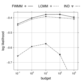
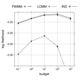
Figure 2: Market maker accuracy, varying the budget level. Left: average over variables. Right: average over bundles. Average taken over all hourly logs and all random seeds.

Accuracy over time

Fig. 3 plots the prediction accuracy of the three markets as time progresses. We set a time limit of 30 minutes for Bregman projection. The first time it successfully completes is only at time stamp ‘2010-03-21 13:58:50’, after 45 games are already settled. We therefore begin the plot at time stamp ‘2010-03-19 00:00:00’, corresponding to 16 settled games, as there is very little difference between LCMM and FWMM before that point. The reason FWMM still exceeds LCMM on occasion before the first projection is due to the extension of the partial outcome afforded by the IP, as explained in Sec. 4.

Each point of the time series represents an average over all variables or bundles defined at that time, including those whose outcomes have been settled. This explains the upwards trends of the plots, culminating at accuracy 0 (a perfect score). The trend is not entirely monotonic, as we see from the bundle log likelihood in the stretch after March 22. The dotted vertical lines indicate the beginning of days on which games are played. On such days, we see that accuracy is initially stable, then sharply increases as the games take course and their outcomes are settled.

In Fig. 3, we see that once Bregman projections successfully complete, the improvement of FWMM over LCMM becomes sustained. The accuracy improvements from this point onwards range from $0\%$ to $80\%$ for variables, with a median of $38\%$ over all hourly summaries. The improvements range from $0\%$ to $44\%$ for bundles, with a median of $9\%$.

Figure 3: Market maker accuracy over time, at budget level 10. Left: average over variables. Right: average over bundles. Average taken over all variables or bundles defined at that time, over all random seeds. The dotted vertical lines are at 00:00 on days when games are played. The solid vertical line indicates the start of projections in FWMM.

6 Discussion and Conclusion

In our experiments, FWMM outperformed LCMM once the outcome space was sufficiently reduced, via settled securities, to allow computing of Bregman projections within 30 minutes on a standard workstation. This time limit yielded a manageable experimental turnaround, with about 5 hours to execute the trades that originally spanned 22 days. In practice, a market designer can allow longer computation and use more powerful hardware, and expect improvements for larger problem sizes.

Several approaches could further speed up our framework. For instance, FW can be used to construct separating hyperplanes to tighten the outer LCMM approximation, and thereby contribute to arbitrage removal even when there is no time to compute the projection. Also, instead of solving IPs to optimality in each iteration, it may be possible to interleave IP with local search to obtain additional descent vertices. Since IP is by far the most time-consuming part of FW, this could yield substantial speedups.

APPENDIX

Appendix A Proof of Proposition 2.4

We first calculate the largest possible guaranteed profit:

$$\adjustlimits{\sup}_{\boldsymbol{\delta}\in\mathbb{R}^{\mathcal{I}}}{\min}_{\boldsymbol{z}\in\mathcal{Z}}\bigl{[}\boldsymbol{\delta}\cdot\boldsymbol{z}-C(\boldsymbol{\theta}+\boldsymbol{\delta})+C(\boldsymbol{\theta})\bigr{]} =\adjustlimits{\sup}_{\boldsymbol{\theta}^{\prime}\in\mathbb{R}^{\mathcal{I}}}{\min}_{{\boldsymbol{\mu}}\in\mathcal{M}}\bigl{[}(\boldsymbol{\theta}^{\prime}-\boldsymbol{\theta})\cdot{\boldsymbol{\mu}}-C(\boldsymbol{\theta}^{\prime})+C(\boldsymbol{\theta})\bigr{]}$$

$$=\adjustlimits{\min}_{{\boldsymbol{\mu}}\in\mathcal{M}}{\sup}_{\boldsymbol{\theta}^{\prime}\in\mathbb{R}^{\mathcal{I}}}\bigl{[}(\boldsymbol{\theta}^{\prime}-\boldsymbol{\theta})\cdot{\boldsymbol{\mu}}-C(\boldsymbol{\theta}^{\prime})+C(\boldsymbol{\theta})\bigr{]}$$ (7)

$$=\min_{{\boldsymbol{\mu}}\in\mathcal{M}}\bigl{[}R({\boldsymbol{\mu}})-\boldsymbol{\theta}\cdot{\boldsymbol{\mu}}+C(\boldsymbol{\theta})\bigr{]}$$ (8)

$$=\min_{{\boldsymbol{\mu}}\in\mathcal{M}}D({\boldsymbol{\mu}}\|\boldsymbol{\theta})=D({\boldsymbol{\mu^{\star}}}\|\boldsymbol{\theta})\enspace,$$ (9)

where Eq. (7) follows by Sion’s minimax theorem and Eqs. (8) and (9) from definitions of the convex conjugate and Bregman divergence, respectively. This shows that from the state $\boldsymbol{\theta}$ the guaranteed profit is at most $D({\boldsymbol{\mu^{\star}}}\|\boldsymbol{\theta}).$

Recall that $\boldsymbol{\delta^{\star}}$ is any trade that moves the market to a state $\boldsymbol{\theta^{\star}}$ such that $\boldsymbol{p}(\boldsymbol{\theta^{\star}})={\boldsymbol{\mu^{\star}}}$. We next show that $\boldsymbol{\delta^{\star}}$ is an optimal trade, i.e., that this trade gives a profit that is at least $D({\boldsymbol{\mu^{\star}}}\|\boldsymbol{\theta}).$ Let $F({\boldsymbol{\mu}})\coloneqq D({\boldsymbol{\mu}}\|\boldsymbol{\theta})$. Since ${\boldsymbol{\mu^{\star}}}$ optimizes $F$ on $\mathcal{M}$, by the first order optimality, we have for any ${\boldsymbol{u}}\in\partial F({\boldsymbol{\mu^{\star}}})$ and $\boldsymbol{z}\in\mathcal{Z}$ that ${\boldsymbol{u}}\cdot(\boldsymbol{z}-{\boldsymbol{\mu^{\star}}})\geq 0$. Since $\boldsymbol{p}(\boldsymbol{\theta^{\star}})={\boldsymbol{\mu^{\star}}}$, the conjugacy implies that $\boldsymbol{\theta^{\star}}\in\partial R({\boldsymbol{\mu^{\star}}})$ and thus $(\boldsymbol{\theta^{\star}}-\boldsymbol{\theta})\in\partial F({\boldsymbol{\mu^{\star}}})$, so the first order optimality yields

$$0\leq(\boldsymbol{\theta^{\star}}-\boldsymbol{\theta})\cdot(\boldsymbol{z}-{\boldsymbol{\mu^{\star}}})\enspace,$$

which rearranges to

$$(\boldsymbol{\theta^{\star}}-\boldsymbol{\theta})\cdot\boldsymbol{z}\geq(\boldsymbol{\theta^{\star}}-\boldsymbol{\theta})\cdot{\boldsymbol{\mu^{\star}}}\enspace.$$ (10)

The profit from the trade $\boldsymbol{\delta^{\star}}$ given any outcome $\omega$ is therefore at least

$$(\boldsymbol{\theta^{\star}}-\boldsymbol{\theta})\cdot\boldsymbol{\phi}(\omega)-C(\boldsymbol{\theta^{\star}})+C(\boldsymbol{\theta}) \geq(\boldsymbol{\theta^{\star}}-\boldsymbol{\theta})\cdot{\boldsymbol{\mu^{\star}}}-C(\boldsymbol{\theta^{\star}})+C(\boldsymbol{\theta})$$

$$=R({\boldsymbol{\mu^{\star}}})-\boldsymbol{\theta}\cdot{\boldsymbol{\mu^{\star}}}+C(\boldsymbol{\theta})$$

$$=D({\boldsymbol{\mu^{\star}}}\|\boldsymbol{\theta})\enspace,$$

where the first line follows by substituting $\boldsymbol{\phi}(\omega)$ for $\boldsymbol{z}$ in Eq. (10), the second line follows from the conjugacy of $R$ and $C$, and the third line from the definition of $D$, completing the proof. ∎

Appendix B Bounded loss property under gradual revelation of outcome

We show that the bound on the worst-case loss of the cost $C$ is maintained if we update the cost function using a sequence of partial outcomes, gradually revealing the final outcome $\omega$. We begin with the worst-case bound on the loss under cost $C$:

Proposition B.1.

If the initial market state is $\boldsymbol{\theta}_{0}$ then the worst-case loss of a market-maker using $C$ is $\max_{\omega\in\Omega}D(\boldsymbol{\phi}(\omega)\|\boldsymbol{\theta}_{0})$.

Proof B.2.

Let $\boldsymbol{\theta}$ denote the final state before the outcome $\omega$ is revealed. Then the market maker has collected $C(\boldsymbol{\theta})-C(\boldsymbol{\theta}_{0})$ as the revenue for the sold shares, and needs to pay out $(\boldsymbol{\theta}-\boldsymbol{\theta}_{0})\cdot\boldsymbol{\phi}(\omega)$ as a payoff to the traders. The worst-case loss is therefore

$$\adjustlimits{\max}_{\omega\in\Omega}{\sup}_{\boldsymbol{\theta}}\Bigl{[}(\boldsymbol{\theta}-\boldsymbol{\theta}_{0})\cdot\boldsymbol{\phi}(\omega)-\bigl{(}C(\boldsymbol{\theta})-C(\boldsymbol{\theta}_{0})\bigr{)}\Bigr{]}$$

$$\quad{}=\adjustlimits{\max}_{\omega\in\Omega}{\sup}_{\boldsymbol{\theta}}\Bigl{[}\bigl{(}\boldsymbol{\theta}\cdot\boldsymbol{\phi}(\omega)-C(\boldsymbol{\theta})\bigr{)}-\boldsymbol{\theta}_{0}\cdot\boldsymbol{\phi}(\omega)+C(\boldsymbol{\theta}_{0})\Bigr{]}$$

$$\quad{}=\max_{\omega\in\Omega}\Bigl{[}R\bigl{(}\boldsymbol{\phi}(\omega)\bigr{)}-\boldsymbol{\theta}_{0}\cdot\boldsymbol{\phi}(\omega)+C(\boldsymbol{\theta}_{0})\Bigr{]}$$

$$\quad{}=\max_{\omega\in\Omega}D(\boldsymbol{\phi}(\omega)\|\boldsymbol{\theta}_{0})\enspace.$$ ∎

Now, we will analyze the case with partial outcomes. We assume that the initial partial outcome $\sigma_{0}=\emptyset$, and that the market goes through a sequence of partial outcomes $\sigma_{0}\subseteq\sigma_{1}\subseteq\dotsb\subseteq\sigma_{T}$ until finally an outcome $\omega$ is revealed, consistent with $\sigma_{T}$. After the revelation of each $\sigma_{t}$, the market-maker switches to the cost function $C_{\sigma_{t}}$. The initial market state is denoted $\boldsymbol{\theta}_{0}$ and the market state in which the market switches to $C_{\sigma_{t}}$ is denoted $\boldsymbol{\theta}_{t}$.

Proposition B.3.

If the initial market state is $\boldsymbol{\theta}_{0}$ then, regardless of the sequence of partial outcomes $\sigma_{1},\dotsc,\sigma_{T}$, the worst-case loss of the market-maker using the sequence of costs $C_{\sigma_{t}}$ is $\max_{\omega\in\Omega}D(\boldsymbol{\phi}(\omega)\|\boldsymbol{\theta}_{0})$, i.e., the same as that of the market-maker using $C$ without incorporating partial outcomes.

Proof B.4.

Recall that the market state at the time of switch from $C_{\sigma_{t-1}}$ to $C_{\sigma_{t}}$ is $\boldsymbol{\theta}_{t}$. We first show that the value of the cost at the time of switch decreases:

$$C_{\sigma_{t}}(\boldsymbol{\theta}_{t})=\sup_{{\boldsymbol{\mu}}\in V_{\sigma_{t}}}\left[\boldsymbol{\theta}\cdot{\boldsymbol{\mu}}-R({\boldsymbol{\mu}})\right]\leq\sup_{{\boldsymbol{\mu}}\in V_{\sigma_{t-1}}}\left[\boldsymbol{\theta}\cdot{\boldsymbol{\mu}}-R({\boldsymbol{\mu}})\right]=C_{\sigma_{t-1}}(\boldsymbol{\theta}_{t})$$ (11)

where the middle inequality follows because $V_{\sigma_{t}}\subseteq V_{\sigma_{t-1}}$. We are now ready to prove the bound on the worst-case loss. Let $\Omega(\sigma_{T})$ denote the set of outcomes compatible with $\sigma_{T}$, and recall that $\sigma_{0}=\emptyset$, so $C_{\sigma_{0}}\equiv C$. Recall that $\boldsymbol{\theta}_{t}$ for $t=1,\dotsc,T$ are the states of the market when the cost becomes $C_{\sigma_{t}}$. Finally, let $\boldsymbol{\theta}_{T+1}$ denote the final state. Then the worst-case loss of the market maker can be bounded as follows

$$\max_{\sigma_{1}\subseteq\sigma_{2}\subseteq\dotsc\subseteq\sigma_{T}\vphantom{\Omega}}\adjustlimits{\max}_{\omega\in\Omega(\sigma_{T})}{\sup}_{\boldsymbol{\theta}_{1},\dotsc,\boldsymbol{\theta}_{T+1}}\left[(\boldsymbol{\theta}_{T+1}-\boldsymbol{\theta}_{0})\cdot\boldsymbol{\phi}(\omega)-\sum_{t=0}^{T}\bigl{(}C_{\sigma_{t}}(\boldsymbol{\theta}_{t+1})-C_{\sigma_{t}}(\boldsymbol{\theta}_{t})\bigr{)}\right]$$

$$\quad{}=\max_{\sigma_{1}\subseteq\sigma_{2}\subseteq\dotsc\subseteq\sigma_{T}\vphantom{\Omega}}\adjustlimits{\max}_{\omega\in\Omega(\sigma_{T})}{\sup}_{\boldsymbol{\theta}_{1},\dotsc,\boldsymbol{\theta}_{T+1}}\biggl{[}(\boldsymbol{\theta}_{T+1}-\boldsymbol{\theta}_{0})\cdot\boldsymbol{\phi}(\omega)-\bigl{(}C_{\sigma_{T}}(\boldsymbol{\theta}_{T+1})-C_{\sigma_{0}}(\boldsymbol{\theta}_{0})\bigr{)}\biggr{.}$$

$$\hskip 162.6075pt\biggl{.}{}-\sum_{t=1}^{T}\bigl{(}C_{\sigma_{t-1}}(\boldsymbol{\theta}_{t})-C_{\sigma_{t}}(\boldsymbol{\theta}_{t})\bigr{)}\biggr{]}$$ (12)

$$\quad{}\leq\max_{\sigma_{T}\vphantom{\Omega}}\adjustlimits{\max}_{\omega\in\Omega(\sigma_{T})}{\sup}_{\boldsymbol{\theta}_{T+1}}\Bigl{[}(\boldsymbol{\theta}_{T+1}-\boldsymbol{\theta}_{0})\cdot\boldsymbol{\phi}(\omega)-C_{\sigma_{T}}(\boldsymbol{\theta}_{T+1})+C_{\sigma_{0}}(\boldsymbol{\theta}_{0})\Bigr{]}$$ (13)

$$\quad{}=\max_{\sigma_{T}\vphantom{\Omega}}\max_{\omega\in\Omega(\sigma_{T})}\Bigl{[}R\bigl{(}\boldsymbol{\phi}(\omega)\bigr{)}-\boldsymbol{\theta}_{0}\cdot\boldsymbol{\phi}(\omega)+C(\boldsymbol{\theta}_{0})\Bigr{]}$$ (14)

$$\quad{}=\max_{\omega\in\Omega}D(\boldsymbol{\phi}(\omega)\|\boldsymbol{\theta}_{0})\enspace.$$ (15)

Eq. (12) follows by rearranging the terms. Eq. (13) follows by Eq. (11). Eq. (14) follows because the convex conjugate of $C_{\sigma_{T}}$ is $R_{\sigma_{T}}({\boldsymbol{\mu}})=\mathbb{I}\{{\boldsymbol{\mu}}\in V_{\sigma_{T}}\}+R({\boldsymbol{\mu}})$, and $R_{\sigma_{T}}\bigl{(}\boldsymbol{\phi}(\omega)\bigr{)}=R\bigl{(}\boldsymbol{\phi}(\omega)\bigr{)}$ thanks to the compatibility of $\omega$ with $\sigma_{T}$. Finally, Eq. (15) follows from the definition of Bregman divergence, completing the proof.

Appendix C Differentiability and controlled growth of $R$

The algorithm used by our market maker requires a differentiable objective whose gradient does not grow too fast as it approaches the boundary of $\mathcal{M}$. Note that for LMSR, the Bregman divergence is formally not even differentiable in its first argument (it is subdifferentiable). So, in addition to requiring the controlled growth of the gradient, we also need to assume that $R$ can be extended into a differentiable function. Specifically, we say that $\bar{R}:\mathbb{R}^{\mathcal{I}}\to(-\infty,\infty]$ is a convex extension of $R$ if $\bar{R}$ is convex and coincides with $R$ wherever $R<\infty$. We require existence of an extension with the controlled growth property in the following sense:

Definition C.1.

Let $\mathcal{S}\subseteq[0,1]^{n}$ be a compact convex set. We say that a convex function $F$ exhibits controlled growth on $\mathcal{S}$ if it is differentiable on $\mathcal{S}\cap(0,1)^{n}$ and if there exists a fixed $p\geq 0$ and $L\geq 0$ such that for any $\varepsilon>0$, the gradient $\nabla F$ has a bounded Lipschitz constant $L_{\varepsilon}\leq L\varepsilon^{-p}$ over $\mathcal{S}\cap[\varepsilon,1-\varepsilon]^{n}$.

Assumption C.2

$R$ has a convex extension $\bar{R}$ such that for all partial outcomes $\sigma$, when $\bar{R}$ is viewed as a function on $V_{\sigma}$, it exhibits controlled growth on $\mathcal{M}_{\sigma}$.

We write $\bar{R}_{\sigma}$ for the restriction of $\bar{R}$ to $V_{\sigma}$. Note that this restriction is formally a function defined on a space of dimension $\lvert\mathcal{I}\backslash\mathcal{I}_{\sigma}\rvert$ and thus, formally, $\nabla\bar{R}_{\sigma}$ has the dimension $\lvert\mathcal{I}\backslash\mathcal{I}_{\sigma}\rvert$. We extend $\nabla\bar{R}_{\sigma}$ into a vector in $\mathbb{R}^{\mathcal{I}}$ by inserting zeros at coordinates $i\in\mathcal{I}_{\sigma}$. A key consequence of this construction is that for any partial outcome $\sigma$ and all ${\boldsymbol{\mu}}\in\mathcal{M}_{\sigma}$ such that $\mu_{i}\in(0,1)$ for $i\not\in\mathcal{I}_{\sigma}$, the gradient $\nabla\bar{R}_{\sigma}({\boldsymbol{\mu}})$ is defined, and $\nabla\bar{R}_{\sigma}({\boldsymbol{\mu}})\in\partial R_{\sigma}({\boldsymbol{\mu}})$. As a result, we have that $\boldsymbol{\theta}=\nabla\bar{R}_{\sigma}({\boldsymbol{\mu}})$ implies that $\nabla C_{\sigma}(\boldsymbol{\theta})={\boldsymbol{\mu}}$ (but not vice versa). Assumption C.2 can be verified for instance by upper-bounding the operator norm of the Hessian, which directly upper-bounds the Lipschitz constant of the gradient.

Example C.3.

Controlled growth for LMSR. We define the extension of negative entropy over the non-negative orthant, $\bar{R}({\boldsymbol{\mu}})=\mathbb{I}\{{\boldsymbol{\mu}}\geq\boldsymbol{0}\}+\sum_{i\in\mathcal{I}}\mu_{i}\log\mu_{i}$, which yields $\bar{R}_{\sigma}({\boldsymbol{\mu}})=\mathbb{I}\{\mu_{i}\geq 0\text{ for all }i\not\in\mathcal{I}_{\sigma}\}+\sum_{i\not\in\mathcal{I}_{\sigma}}\mu_{i}\log\mu_{i}$. The Hessian is a diagonal matrix with entries $1/\mu_{i}$, so its operator norm is $\max_{i\not\in\mathcal{I}_{\sigma}}1/\mu_{i}$, and thus $L_{\varepsilon}=O(1/\varepsilon)$, which satisfies the controlled growth condition with $p=1$.

Appendix D Proof of Proposition 4.1

The guaranteed profit when moving from $\boldsymbol{\theta}$ to $\boldsymbol{\hat{\theta}}$ is

$$\min_{\omega\in\Omega}\Bigl{[}(\boldsymbol{\hat{\theta}}-\boldsymbol{\theta})\cdot\boldsymbol{\phi}(\omega)-C(\boldsymbol{\hat{\theta}})+C(\boldsymbol{\theta})\Bigr{]}$$

$$\qquad{}=\min_{{\boldsymbol{\mu}}\in\mathcal{M}}\Bigl{[}(\boldsymbol{\hat{\theta}}-\boldsymbol{\theta})\cdot{\boldsymbol{\mu}}-C(\boldsymbol{\hat{\theta}})+C(\boldsymbol{\theta})\Bigr{]}$$ (16)

$$\qquad{}=\min_{{\boldsymbol{\mu}}\in\mathcal{M}}\Bigl{[}(\boldsymbol{\hat{\theta}}-\boldsymbol{\theta})\cdot({\boldsymbol{\mu}}-\hat{{\boldsymbol{\mu}}})+\boldsymbol{\hat{\theta}}\cdot\hat{{\boldsymbol{\mu}}}-C(\boldsymbol{\hat{\theta}})-\boldsymbol{\theta}\cdot\hat{{\boldsymbol{\mu}}}+C(\boldsymbol{\theta})\Bigr{]}$$

$$\qquad{}=\min_{{\boldsymbol{\mu}}\in\mathcal{M}}\Bigl{[}(\boldsymbol{\hat{\theta}}-\boldsymbol{\theta})\cdot({\boldsymbol{\mu}}-\hat{{\boldsymbol{\mu}}})+R(\hat{{\boldsymbol{\mu}}})-\boldsymbol{\theta}\cdot\hat{{\boldsymbol{\mu}}}+C(\boldsymbol{\theta})\Bigr{]}$$ (17)

$$\qquad{}=D(\hat{{\boldsymbol{\mu}}}\|\boldsymbol{\theta})-g(\hat{{\boldsymbol{\mu}}})\enspace.$$ (18)

Eq. (16) follows because the minimized objective is linear in $\boldsymbol{\phi}(\omega)$. Eq. (17) follows from the definition of $R$. Finally, Eq. (18) follows because $\nabla F(\hat{{\boldsymbol{\mu}}})=\nabla\bar{R}(\hat{{\boldsymbol{\mu}}})-\boldsymbol{\theta}=\boldsymbol{\hat{\theta}}-\boldsymbol{\theta}$, and hence

$$g(\hat{{\boldsymbol{\mu}}})=\max_{{\boldsymbol{\mu}}\in\mathcal{M}}\Bigl{[}(\boldsymbol{\hat{\theta}}-\boldsymbol{\theta})\cdot(\hat{{\boldsymbol{\mu}}}-{\boldsymbol{\mu}})\Bigr{]}\enspace.$$ ∎

References

- [1]
- Abernethy et al. [2011] Jacob Abernethy, Yiling Chen, and Jennifer Wortman Vaughan. 2011. An optimization-based framework for automated market-making. In EC-11.
- Belanger et al. [2013] David Belanger, Dan Sheldon, and Andrew McCallum. 2013. Marginal Inference in MRFs using Frank-Wolfe. In NIPS 2013 workshop on Greedy Optimization, Frank-Wolfe and Friends.
- Berg et al. [2008] Joyce Berg, Robert Forsythe, Forrest Nelson, and Thomas Rietz. 2008. Results from a Dozen Years of Election Futures Markets Research. In Handbook of Exp. Econ. Results.
- Bertsekas [2015] Dimitri P. Bertsekas. 2015. Convex Optimization Algorithms.
- Charette [2007] Robert Charette. 2007. An Internal Futures Market. Information Management (March 2007).
- Chen et al. [2008] Yiling Chen, Lance Fortnow, Nicolas Lambert, David M. Pennock, and Jennifer Wortman. 2008. Complexity of Combinatorial Market Makers. In EC-08.
- Chen et al. [2007] Yiling Chen, Lance Fortnow, Evdokia Nikolova, and David M. Pennock. 2007. Betting on Permutations. In EC-07.
- Chen et al. [2008] Yiling Chen, Sharad Goel, and David M. Pennock. 2008. Pricing Combinatorial Markets for Tournaments. In STOC-08.
- Chen and Pennock [2007] Yiling Chen and David M. Pennock. 2007. A Utility Framework for Bounded-Loss Market Makers. In UAI-07.
- Dudík et al. [2014] Miroslav Dudík, Rafael Frongillo, and Jennifer Wortman Vaughan. 2014. Market Making with Decreasing Utility for Information. In UAI-14.
- Dudík et al. [2012] Miroslav Dudík, Sébastien Lahaie, and David M. Pennock. 2012. A Tractable Combinatorial Market Maker Using Constraint Generation. In EC-12.
- Dudík et al. [2013] Miroslav Dudík, Sébastien Lahaie, David M. Pennock, and David Rothschild. 2013. A Combinatorial Prediction Market for the U.S. Elections. In EC-13.
- Frank and Wolfe [1956] Marguerite Frank and Philip Wolfe. 1956. An algorithm for quadratic programming. Naval research logistics quarterly 3, 1-2 (1956).
- Hanson [2003] Robin D. Hanson. 2003. Combinatorial information market design. Information Systems Frontiers 5, 1 (2003).
- Hanson [2007] Robin D. Hanson. 2007. Logarithmic market scoring rules for modular combinatorial information aggregation. Journal of Prediction Markets 1, 1 (2007).
- Jaggi [2013] Martin Jaggi. 2013. Revisiting Frank-Wolfe: Projection-free sparse convex optimization. In ICML-13.
- Krishnan et al. [2015] Rahul G. Krishnan, Simon Lacoste-Julien, and David Sontag. 2015. Barrier Frank-Wolfe for marginal inference. In NIPS-15.
- Nesterov [2007] Yurii Nesterov. 2007. Gradient methods for minimizing composite objective function. Technical Report. UCL.
- Pennock et al. [2002] David M. Pennock, Steve Lawrence, C. Lee Giles, and Finn A. Nielsen. 2002. The real power of artificial markets. Science 291 (2002).
- Spann and Skiera [2003] Martin Spann and Bernd Skiera. 2003. Internet-Based Virtual Stock Markets for Business Forecasting. Management Science 49, 10 (2003).
- Xia and Pennock [2011] Lirong Xia and David M. Pennock. 2011. An Efficient Monte-Carlo Algorithm for Pricing Combinatorial Prediction Markets for Tournaments. In IJCAI-11.