Measurement of the Top Quark Mass Using the Matrix Element Technique in Dilepton Final States.

Abstract

We present a measurement of the top quark mass in $p\bar{p}$ collisions at a center-of-mass energy of 1.96 TeV at the Fermilab Tevatron collider. The data were collected by the D0 experiment corresponding to an integrated luminosity of 9.7 fb^-1. The matrix element technique is applied to $t\bar{t}$ events in the final state containing leptons (electrons or muons) with high transverse momenta and at least two jets. The calibration of the jet energy scale determined in the lepton + jets final state of $t\bar{t}$ decays is applied to jet energies. This correction provides a substantial reduction in systematic uncertainties. We obtain a top quark mass of $m_{t}=173.93\pm 1.84$ GeV.

I Introduction

The top quark is the heaviest elementary particle of the standard model (SM) Abazov et al. (2014a, 2015); CDF and D0 collaborations (2014); Khachatryan et al. (2016); ATLAS Collaboration, CDF Collaboration, CMS Collaboration, and D0 Collaboration (2014). Its mass ($m_{t}$) is a free parameter of the SM Lagrangian that is not predicted from first principles. The top quark was discovered in 1995 by the CDF and D0 Collaborations at the Tevatron $p\bar{p}$ collider at Fermilab Abachi et al. (1995); Abe et al. (1995). Despite the fact that the top quark decays weakly, its large mass leads to a very short lifetime of approximately $5\cdot 10^{-25}$ s Jezabek and Kühn (1988, 1989); Abazov et al. (2012a). It decays into a $W$ boson and a $b$ quark before hadronizing, a process that has a characteristic time scale of $1/\Lambda_{\rm{QCD}}\approx(200~{}{\rm MeV})^{-1}$, equivalent to $\tau_{\rm{had}}\approx 3.3\cdot 10^{-24}$ s, where $\Lambda_{\rm{QCD}}$ is the fundamental scale of quantum chromodynamics (QCD). This provides an opportunity to measure the mass of the top quark with high precision due to possibility of reconstructing the top quark parameters using its decay particles.

At the Tevatron, top quarks are produced mainly as $t\bar{t}$  pairs through the strong interaction. At leading order (LO) in perturbative QCD, a pair of top quarks is produced via quark-antiquark ($q\bar{q}$) annihilation with a probability of about 85% Bernreuther et al. (2004); Czakon et al. (2013), or via gluon-gluon ($gg$) fusion.

Final states of $t\bar{t}$  production are classified according to the decays of the two $W$ bosons. This results in final states with two, one, or no leptons, which are referred to as the dilepton ($\ell\ell$), lepton + jets ($\ell$+jets), and all-jet channels, respectively. In this measurement we use events in the dilepton final state where both $W$ bosons decay to leptons: $t\bar{t}\to W^{+}b\ W^{-}\bar{b}\to\ell^{+}\nu_{\ell}b\ \ell^{-}\bar{\nu_{\ell}}\bar{b}$. More specifically, we consider three combinations of leptons, $ee$, $e\mu$, and $\mu\mu$, including also electrons and muons from leptonic decays of $\tau$ leptons, $W\to\tau\nu_{\tau}\to\ell\nu_{\ell}\nu_{\tau}$. We present an updated measurement of the top quark mass in the dilepton channel using the matrix element (ME) approach  Abazov et al. (2004). This measurement improves the previous result using the matrix element technique with 5.3 fb^-1 of integrated luminosity Abazov et al. (2011b) by a factor of 1.6, where the statistical uncertainty is improved by a factor of 1.1 and systematic uncertainty by a factor of 2.7. The most precise $m_{t}$ measurement by D0 experiment based on this method was performed in $\ell$+jets analysis  Abazov et al. (2014a, 2015). The CMS Collaboration has applied a different approach for measuring $m_{t}$ in the dilepton channel, obtaining a precision of 1.23 GeV Khachatryan et al. (2016).

This measurement uses the entire data set accumulated by the D0 experiment during Run II of the Fermilab Tevatron collider, corresponding to an integrated luminosity of 9.7 fb^-1. We use the final D0 jet energy scale (JES) corrections and the refined corrections of the $b$ quark jet energy scale Abazov et al. (2014b). The measurement is performed with a blinded approach, as described in Section IV. Similarly to the recent top mass measurement in the dilepton final state using a neutrino weighting technique Abazov et al. (2016), we correct jet energies by a calibration factor obtained in the top quark mass measurement in the $\ell$+jets analysis Abazov et al. (2014a, 2015).

II Detector and event samples

II.1 D0 detector

The D0 detector is described in detail in Refs. Abazov et al. (2006, 2005); Abolins et al. (2008); Angstadt et al. (2010); Ahmed et al. (2011); Casey et al. (2013); Bezzubov et al. (2014). It has a central tracking system consisting of a silicon microstrip tracker and a central fiber tracker, both located within a 2 T superconducting solenoidal magnet. The central tracking system is designed to optimize tracking and vertexing at detector pseudorapidities of $|\eta_{\text{det}}|<2.5$. A liquid-argon sampling calorimeter has a central section (CC) covering $|\eta_{\text{det}}|$ up to $\approx 1.1$, and two end calorimeters (EC) that extend coverage to $|\eta_{\text{det}}|\approx 4.2$, with all three housed in separate cryostats. An outer muon system, with pseudorapidity coverage of $|\eta_{\text{det}}|<2$, consists of a layer of tracking detectors and scintillation trigger counters in front of 1.8 T iron toroids, followed by two similar layers after the toroids.

The sample of $p\bar{p}$ collision data considered in this analysis is split into four data-taking periods: “Run IIa”, “Run IIb1”, “Run IIb2”, and “Run IIb3” with the corresponding integrated luminosities given in Table I. All event simulations are split according to these epochs to better model changes of detector response with time, such as the addition of an additional SMT layer Angstadt et al. (2010)or the reconstruction algorithm performance variations due to increasing luminosity Abazov et al. (2014c).

II.2 Object identification

Top pair events in the dilepton channel contain two isolated charged leptons, two $b$ quark jets, and a significant imbalance in transverse momentum ($/\kern-5.50003ptp_{T}$) due to escaping neutrinos.

Electrons are identified as energy clusters in the calorimeter within a cone of radius ${\cal R}=\sqrt{(\Delta\eta)^{2}+(\Delta\phi)^{2}}=0.2$ (where $\phi$ is the azimuthal angle) that are consistent in their longitudinal and transverse profiles with expectations from electromagnetic showers. More than 90% of the energy of an electron candidate must be deposited in the electromagnetic part of the calorimeter. The electron is required to be isolated by demanding that less than $20$% of its energy is deposited in an annulus of $0.2<{\cal R}<0.4$ around its direction. This cluster has to be matched to a track reconstructed in the central tracking system. We consider electrons in the CC with $|\eta_{\text{det}}|<1.1$ and in the EC with $1.5<|\eta_{\text{det}}|<2.5$. The transverse momenta of electrons ($p_{T}^{e}$) must be greater than $15$ GeV. In addition, we use a multivariate discriminant based on tracking and calorimeter information to reject jets misidentified as electrons. It has an electron selection efficiency between 75% and 80%, depending on the data taking period, rapidity of the electron, and number of jets in the event. The rejection rate for jets is approximately $96$%.

Muons are identified Abazov et al. (2014c) as segments in at least one layer of the muon system that are matched to tracks reconstructed in the central tracking system. Reconstructed muons must have $p_{T}>15$ GeV, $|\eta|<2$, and satisfy the two following isolation criteria. First, the transverse energy deposited in the calorimeter annulus $0.1<{\cal R}<0.4$ around the muon ($E_{T}^{\mu,\text{iso}}$) must be less than 15% of the transverse momentum of the muon ($p^{\mu}_{T}$). Secondly, the sum of the transverse momenta of the tracks in a cone of radius ${\cal R}=0.5$ around the muon track in the central tracking system ($p_{T}^{\mu,\text{iso}}$) must be less than 15% of $p^{\mu}_{T}$.

Jets are identified as energy clusters in the electromagnetic and hadronic parts of the calorimeter, reconstructed using an iterative mid-point cone algorithm with radius ${\cal R}=0.5$ Blazey et al. (2000). An external JES correction is determined by calibrating the energy deposited in the jet cone using transverse momentum balance in exclusive photon+jet and dijet events in data Abazov et al. (2014b). When a muon track overlaps the jet cone, twice the $p_{T}$ of the muon is added to the jet $p_{T}$, assuming that the muon originates from a semileptonic decay of a hadron belonging to the jet and that the neutrino has the same $p_{T}$ as the muon. In addition, we use the difference in single-particle responses between data and Monte Carlo (MC) simulation to provide a parton-flavor dependent JES correction Abazov et al. (2014b). This correction significantly reduces the bias in the jet energy and the total JES uncertainty of the jets initiated by $b$ quarks. Jet energies in simulated events are also corrected for residual differences in energy resolution and energy scale between data and simulation. These correction factors are measured by comparing data and simulation in Drell$-$Yan ($\mbox{$Z/\gamma^{\star}$}\to ee$) events with accompanying jets Abazov et al. (2014b).

The typical JES uncertainty is approximately $2\%$. We improve this by calibrating the jet energy after event selection through a constant scale factor $k_{\rm JES}$ measured in the lepton+jets final state using jets associated with $W$ boson decay Abazov et al. (2014a, 2015). This approach was first applied in Ref. Abazov et al. (2012b). We apply the $k_{\rm JES}$ factor to the jet $p_{T}$ in data as $p^{\rm corr}_{T}=p_{T}/k_{\rm JES}$, independently for each data taking period. We use the correction factors averaged over $e$+jets and $\mu$+jets final states (Table 1). The uncertainties related to the determination and propagation of the $k_{\rm JES}$ scale factor are accounted for as systematic uncertainties and described in Section V.

Data taking period	Integrated luminosity, pb-1	$k_{\rm JES}$
RunIIa	1081	0.993 $\pm$ 0.016
RunIIb1	1223	1.027 $\pm$ 0.013
RunIIb2	3034	1.033 $\pm$ 0.008
RunIIb3	4398	1.026 $\pm$ 0.006

Table 1: The integrated luminosity and the jet energy scale correction factor $k_{\rm JES}$, averaged over $e$+jets and $\mu$+jets channels Abazov et al. (2014a, 2015), for the four separate data taking periods.

We use a multivariate analysis (MVA) technique to identify jets originating from $b$ quarks Abazov et al. (2010, 2014d). The algorithm combines the information from the impact parameters of tracks and from variables that characterize the properties of secondary vertices within jets. Jet candidates for $b$ tagging are required to have at least two tracks with $p_{T}>0.5$ GeV originating from the vertex of the $p\bar{p}$ interaction, and to be matched to a jet reconstructed from just the charged tracks.

The missing transverse momentum, $/\kern-5.50003ptp_{T}$, is reconstructed from the energy deposited in the calorimeter cells, and all corrections to $p_{T}$ for leptons and jets are propagated into a revised $/\kern-5.50003ptp_{T}$. A significance in $/\kern-5.50003ptp_{T}$, symbolized by $\sigma_{/\kern-2.79996ptp_{T}}$, is defined through a likelihood ratio based on the $/\kern-5.50003ptp_{T}$ probability distribution, calculated from the expected resolution in $/\kern-5.50003ptp_{T}$ and the energies of electrons, muons, and jets.

II.3 Event selection

We follow the approach developed in Ref. Abazov et al. (2011a) to select dilepton events, using the criteria listed below:

1. For the $ee$ and $\mu\mu$ channels, we select events that pass at least one single-lepton trigger, while for the $e\mu$ channel we consider events selected through a mixture of single and multilepton triggers and lepton+jet triggers. Efficiencies for single electron and muon triggers are measured using $\mbox{$Z/\gamma^{\star}$}\to ee$ or $\mbox{$Z/\gamma^{\star}$}\to\mu\mu$ data, and found to be $\approx 99$% and $\approx 80$%, respectively, in dilepton events. For the $e\mu$ channel, the trigger efficiency is $\approx$ 100%.

2. We require at least one $p\bar{p}$ interaction vertex in the interaction region with $|z|<60$ cm, where $z$ is the coordinate along the beam axis, and $z=0$ is the center of the detector. At least three tracks with $p_{T}>0.5$ GeV must be associated with this vertex.

3. We require at least two isolated leptons with $\mbox{$p_{T}$}>15$ GeV, both originating from the same interaction vertex. The two highest-$p_{T}$ leptons must have opposite electric charges.

4. To reduce the background from bremsstrahlung in the $e\mu$ final state, we require the distance in ($\eta,\phi$) space between the electron and the muon trajectories to be ${\cal R}(e,\mu)>0.3$.

5. We require the presence of at least two jets with $\mbox{$p_{T}$}>20$ GeV and $|\eta_{\text{det}}|<2.5$.

6. The $t\bar{t}$ final state contains two $b$ quark jets. To improve the separation between signal and background, we apply a selection using the $b$ quark jet identification MVA discriminant to demand that at least one of the two jets with highest $p_{T}$ is $b$ tagged Abazov et al. (2010, 2014d). The $b$ tagging helps significantly in rejecting Z boson related backgrounds. We apply requirements on the MVA variable that provide $b$ quark jet identification efficiencies of 84% in $e\mu$, 80% in $ee$, and 78% in $\mu\mu$ final states, with background misidentifications rates of 23%, 12%, and 7%, respectively.

7. Additional selection criteria based on global event properties further improve the signal purity. In $e\mu$ events, we require $H_{T}>110$ GeV, where $H_{T}$ is the scalar sum of the $p_{T}$ of the leading lepton and the two leading jets. In the $ee$ final state, we require $\sigma_{/\kern-2.79996ptp_{T}}$$>5$, while in the $\mu\mu$ channel, we require $/\kern-5.50003ptp_{T}$$>40$ GeV and $\sigma_{/\kern-2.79996ptp_{T}}$$>2.5$.

8. In rare cases, the numerical integration of the matrix elements described in Section III.1 may yield extremely small probabilities that prevent us from using the event in the analysis. We reject such events using a selection that has an efficiency of 99.97% for simulated $t\bar{t}$ signal samples. For background MC events, the efficiency is 99.3%. No event is removed from the final data sample because of this requirement.

II.4 Simulation of signal and background events

The main sources of background in the $\ell\ell$  channel are Drell$-$Yan production ($q\bar{q}\to(\mbox{$Z/\gamma^{\star}$}\to\ell\ell)$+jets), diboson production (WW, WZ, and ZZ), and instrumental background. The instrumental background arises mainly from $(W\to\ell\nu)$+jets and multijet events, in which one or two jets are misidentified as electrons, or where muons or electrons originating from semileptonic decays of heavy-flavor hadrons appear to be isolated. To estimate the $t\bar{t}$ signal efficiency and the background contamination, we use MC simulation for all contributions, except for the instrumental background, which is estimated from data.

The number of expected $t\bar{t}$ signal events is estimated using the LO matrix element generator alpgen (version v2.11) Mangano et al. (2003) for the hard-scattering process, with up to two additional partons, interfaced with the pythia generator Sjöstrand et al. (2006) (version 6.409, with a D0 modified Tune A Affolder et al. (2002)) for parton showering and hadronization. The CTEQ6M parton distribution functions (PDF) Pumplin et al. (2002); Nadolsky et al. (2008) are used in the event generation, with the top quark mass set to 172.5 GeV. The next-to-next-to LO (NNLO) $t\bar{t}$ cross section of $7.23^{+0.11}_{-0.20}$ pb Czakon and Mitov (2014) is used for the normalization. For the calibration of the ME method, we also use events generated at $m_{t}=$ 165 GeV, 170 GeV, 175 GeV, and 180 GeV. Those samples are simulated in the same way as the sample with the $m_{t}=172.5$ GeV. Drell$-$Yan samples are also simulated using alpgen (version 2.11) for the hard-scattering process, with up to three additional partons, and the pythia (version 6.409, D0 modified Tune A) generator for parton showering and hadronization. We separately generate processes corresponding to $Z$-boson production with heavy flavor partons, $(Z\to\ell\ell)+b\bar{b}$ and $(Z\to\ell\ell)+c\bar{c}$, and light flavor partons. Samples with light partons only are generated separately for the parton multiplicities of 0, 1, 2 and 3, samples with the heavy flavor partons are generated including additional 0, 1 and 2 light partons. The MC cross sections for all Drell$-$Yan samples are scaled up with a next-to-LO (NLO) $K$-factor of 1.3, and cross sections for heavy-flavor samples are scaled up with additional $K$-factors of 1.52 for $(Z\to\ell\ell)+b\bar{b}$ and 1.67 for $(Z\to\ell\ell)+c\bar{c}$, as estimated with the MCFM program Ellis (2006). In the simulation of diboson events, the pythia generator is used for both hard scattering and parton showering. To simulate effects from additional overlapping $p\bar{p}$ interactions, “zero bias” events are selected randomly in collider data and overlaid on the simulated events. Generated MC events are processed using a geant3-based Brun and Carminati (1993) simulation of the D0 detector.

II.5 Estimation of instrumental background contributions

In the $ee$ and $e\mu$ channels, we determine the contributions from events in data with jets misidentified as electrons through the “matrix method” Abazov et al. (2007). A sample of events ($n_{\text{loose}}$) is defined using the same selections as given for $t\bar{t}$ candidates in items (i) – (vii) above, but omitting the requirement on the electron MVA discriminant. For the dielectron channel, we drop the MVA requirement on one of the randomly-chosen electrons.

Using $\mbox{$Z/\gamma^{\star}$}\to ee$ data, we measure the efficiency $\varepsilon_{e}$ that events with electrons must pass the requirements on the electron MVA discriminant. We measure the efficiency $f_{e}$ that events with no electron pass the electron MVA requirement by using $e\mu$ events selected with criteria (i) – (v), but requiring leptons of same electric charge. We also apply a reversed isolation requirement to the muon, $E^{\mu,\text{iso}}_{T}/p^{\mu}_{T}>0.2$, $p^{\mu,\text{iso}}_{T}/p^{\mu}_{T}>0.2$, and $\mbox{$/\kern-5.50003ptp_{T}$}<15$ GeV, to minimize the contribution from $W$+jets events.

We extract the number of events with misidentified electrons ($n_{f}$), and the number of events with true electrons ($n_{e}$), by solving the equations

$$n_{\text{{loose}}} =n_{e}/\varepsilon_{e}+n_{f}/f_{e},$$ (1)

$$n_{\text{tight}} =n_{e}+n_{f},$$

where $n_{\text{tight}}$ is the number of events remaining after implementing selections (i) – (vii). The factors $f_{e}$ and $\varepsilon_{e}$ are measured for each jet multiplicity (0, 1, and 2 jets), and separately for electron candidates in the central and end sections of the calorimeter. Typical values of $\varepsilon_{e}$ are 0.7 – 0.8 in the CC and 0.65 – 0.75 in the EC. Values of $f_{e}$ are 0.005 – 0.010 in the CC, and 0.005 – 0.020 in the EC.

In the $e\mu$ and $\mu\mu$ channels, we determine the number of events with an isolated muon arising from decays of hadrons in jets by relying on the same selection as for the $e\mu$ or $\mu\mu$ channels, but requiring that both leptons have the same charge. In the $\mu\mu$ channel, the number of background events is taken to be the number of same-sign events. In the $e\mu$ channel, it is the number of events in the same-sign sample after subtracting the contribution from events with misidentified electrons in the same way as it is done in Ref. Abazov et al. (2013).

To use the ME technique, we need a pool of events to calculate probabilities corresponding to the instrumental background. In the $e\mu$ channel, we use the loose sample defined above to model misidentified electron background. Using this selection we obtain a background sample of 2901 events. In the $\mu\mu$ channel, the estimated number of multijet and $W$+jets background events is zero (Table 2). In the $ee$ channel, the number of such events is too small to provide a representative instrumental background sample. Instead we increase the number of background events due to $Z$-boson production by the corresponding amount in the calibration procedure.

II.6 Sample composition

The numbers of predicted background events as well as the expected numbers of signal events for the final selection in $e\mu$, $\mu\mu$, and $ee$ channels are given in Table 2. They show the high signal purity of the selected sample. The $e\mu$ channel has a relatively low fraction of the $Z/\gamma^{\star}$+jets background events because the electron and muon are produced through the cascade decay of the $\tau$-lepton, $\mbox{$Z/\gamma^{\star}$}\to\tau\tau\to e\mu\nu_{e}\nu_{\mu}$. Comparisons between distributions measured in data and predictions after the final selection are shown in Figs. 2-4 for the combined $ee$, $e\mu$, and $\mu\mu$ channels. Only statistical uncertainties are shown. The predicted number of $t\bar{t}$ and background events is normalized to the number of events found in data. The jet $p_{T}$ and $H_{T}$ distributions in Figs. 4 and 4 are shown after applying the $k_{\rm JES}$ correction from the $\ell$+jets analysis Abazov et al. (2014a, 2015).

	$Z/\gamma^{\star}$ + jets	Diboson	Instr.	$t\bar{t}$	Total	Data
$e\mu$	$13.0^{+1.7}_{-1.6}$	$3.7^{+0.8}_{-0.8}$	$16.4^{+4.0}_{-4.0}$	$260.6^{+22.5}_{-16.3}$	$293.8^{+23.5}_{-17.7}$	346
$ee$	$13.8^{+2.1}_{-1.9}$	$1.9^{+0.4}_{-0.4}$	$1.8^{+0.2}_{-0.2}$	$88.0^{+9.1}_{-8.2}$	$105.5^{+10.3}_{-9.5}$	104
$\mu\mu$	$10.6^{+1.3}_{-1.4}$	$1.7^{+0.4}_{-0.4}$	$0^{+0.05}_{-0.05}$	$76.0^{+6.2}_{-4.1}$	$88.3^{+6.7}_{-4.7}$	92
$\ell\ell$	$37.4^{+5.1}_{-4.9}$	$7.3^{+1.6}_{-1.6}$	$18.2^{+4.0}_{-4.0}$	$424.6^{+37.8}_{-28.6}$	$487.6^{+40.5}_{-31.9}$	545

Table 2: The numbers of expected background and $t\bar{t}$ events, and the number of events observed in data. The NNLO cross section is used to normalize the $t\bar{t}$ content. Systematic uncertainties are shown for all the expected numbers.

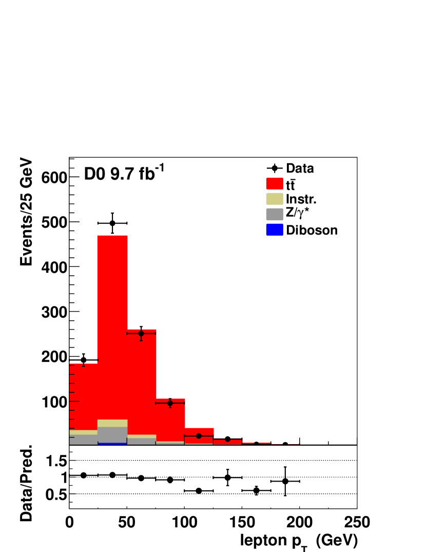
Figure 1: The distributions in lepton $p_{T}$ and the ratio of data to predictions for the combined $ee$, $e\mu$, and $\mu\mu$ final states after applying requirements (i) – (vii).

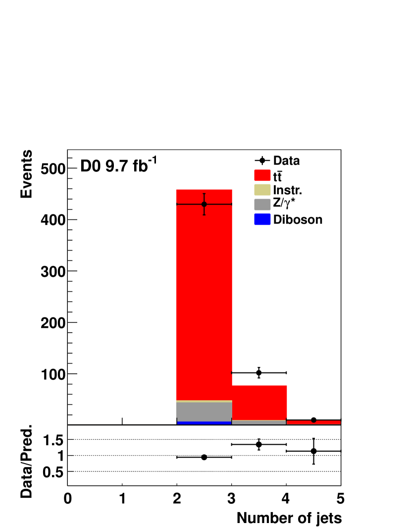
Figure 2: The distributions in the number of jets and the ratio of data to the prediction for the combined $ee$, $e\mu$, and $\mu\mu$ final states after applying requirements (i) – (vii).

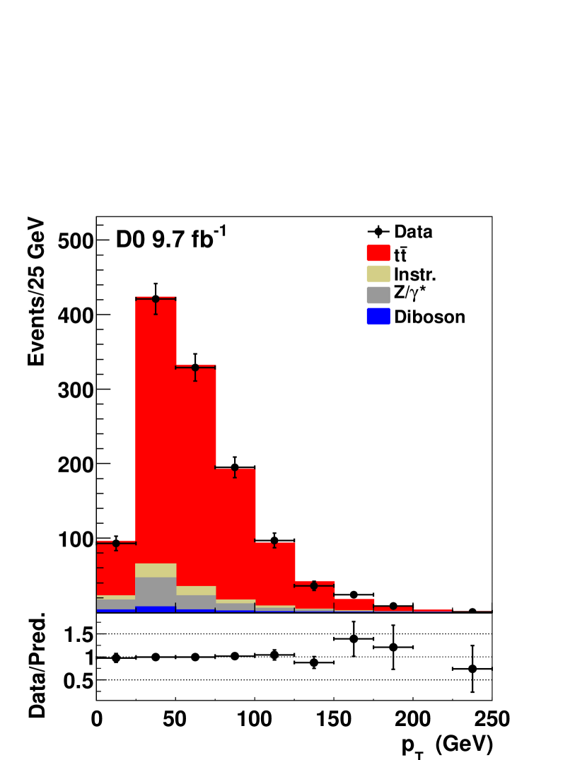
Figure 3: The distributions in jet $p_{T}$ after implementing the $k_{\rm JES}$ correction, and the ratio of data to the prediction for the combined $ee$, $e\mu$, and $\mu\mu$ final states after applying requirements (i) – (vii).

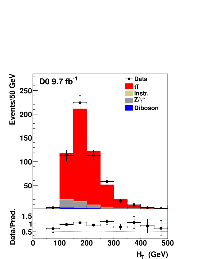
Figure 4: The distributions in $H_{T}$ after implementing the $k_{\rm JES}$ correction, and the ratio of data to the prediction for the combined $ee$, $e\mu$, and $\mu\mu$ final states after applying requirements (i) – (vii).

III MASS DETERMINATION Method

III.1 Matrix Element Technique

This measurement uses the matrix element technique Abazov et al. (2004). This method provides the most precise $m_{t}$ measurement at the Tevatron in the $\ell$+jets final state Abazov et al. (2014a, 2015), and was applied in previous measurement of $m_{t}$ in the dilepton final state using 5.3 fb^-1 of integrated luminosity Abazov et al. (2011b). The ME method used in this analysis is described below.

III.2 Event probability calculation

The ME technique assigns a probability to each event, which is calculated as

$$P(x,f_{t\bar{t}},m_{t})=f_{t\bar{t}}\cdot P_{t\bar{t}}(x,m_{t})+(1-f_{t\bar{t}})\cdot P_{\rm bkg}(x),$$ (2)

where $f_{t\bar{t}}$ is the fraction of $t\bar{t}$ events in the data, and $P_{t\bar{t}}$ and $P_{\rm bkg}$ are the respective per-event probabilities calculated under the hypothesis that the selected event is either a $t\bar{t}$ event, characterized by a top quark mass $m_{t}$, or background. Here, $x$ represents the set of measured observables, i.e., $p_{T}$, $\eta$, and $\phi$ for jets and leptons. We assume that the masses of top quarks and anti-top quarks are the same. The probability $P_{t\bar{t}}(x,m_{t})$ is calculated as

$$\begin{split}P_{t\bar{t}}(x,m_{t})=\frac{1}{\sigma_{\rm obs}(m_{t})}\int f_{\rm PDF}(q_{1})f_{\rm PDF}(q_{2})\times\\ \times\frac{(2\pi)^{4}|\mathscr{M}(y,m_{t})|^{2}}{q_{1}q_{2}s}W(x,y)d\Phi_{6}dq_{1}dq_{2},\end{split}$$ (3)

where $q_{1}$ and $q_{2}$ represent the respective fractions of proton and antiproton momenta carried by the initial state partons, $f_{{\rm PDF}}$ represents the parton distribution functions, and $y$ refers to partonic four-momenta of the final-state objects. The detector transfer functions (TF), $W(x,y)$, correspond to the probability for reconstructing parton four-momenta $y$ as the final-state observables $x$. The term $d\Phi_{6}$ represents the six-body phase space, and $\sigma_{\rm obs}(m_{t})$ is the $t\bar{t}$  cross section observed at the reconstruction level, calculated using the matrix element $\mathscr{M}(y,m_{t})$, corrected for selection efficiency. The LO matrix element $\mathscr{M}(y,m_{t})$ for the processes $q\bar{q}\to t\bar{t}\to W^{+}W^{-}b\bar{b}\to\ell^{+}\ell^{-}\nu_{\ell}\bar{\nu_{\ell}}b\bar{b}$ is used in our calculation Mahlon and Parke (1997) and it contains a Breit-Wigner function to represent each $W$ boson and top quark mass. The matrix element is averaged over the colors and spins of the initial state partons, and summed over the colors and spins of the final state partons. The $gg$ matrix element is neglected, since it comprises only 15% of the total $t\bar{t}$ production cross-section at the Tevatron. Including it does not significantly improve the statistical sensitivity of the method.

The electron momenta and the directions of all reconstructed objects are assumed to be perfectly measured and are therefore represented through $\delta$ functions, $\delta(x-y)$, reducing thereby the dimensionality of the integration. This leaves the magnitues of the jet and muon momenta to be modelled. Following the same approach as in the previous measurement Abazov et al. (2011b), we parametrize the jet energy resolution by a sum of two Gaussian functions with parameters depending linearly on parton energies, while the resolution in the curvature of the muon ($1/p^{\mu}_{T}$) is described by a single Gaussian function. All TF parameters are determined from simulated $t\bar{t}$ events. We use the same parametrizations for the transfer functions as in the $\ell$+jets $m_{t}$ measurement. The detailed description of the TFs is given in Ref. Abazov et al. (2015).

The masses of the six final state particles are set to 0 except for the $b$ quark jets, for which a mass of 4.7 GeV is used. We integrate over 8 dimensions in the $ee$ channel, 9 in the $e\mu$ channel, and 10 in the $\mu\mu$ channel. As integration variables we use the top and antitop quark masses, the $W^{+}$ and $W^{-}$ boson masses, the transverse momenta of the two jets, the $p_{T}$ and $\phi$ of the $t\bar{t}$ system, and $1/p^{\mu}_{T}$ for muons. This choice of variables differs from that of the previous measurement Abazov et al. (2011b), providing a factor of $\approx 100$ reduction in integration time.

To reconstruct the masses of the top quarks and $W$ bosons, we solve the kinematic equations analytically by summing over the two possible jet-parton assignments and over all real solutions for each neutrino momentum Fiedler et al. (2010). If more than two jets exist in the event, we use only the two with highest transverse momenta. The integration is performed using the MC based numerical integration algorithm VEGAS Lepage (1978, 1980), as implemented in the GNU Scientific Library Galassi et al. (2009).

Since the dominant source of background in the dilepton final state is from $\mbox{$Z/\gamma^{\star}$}+\rm jets$ events, as can be seen from Table 2, we consider only the $\mbox{$Z/\gamma^{\star}$}+\rm jets$ matrix element in the calculation of the background probability, $P_{\rm bkg}(x)$. The LO $(\mbox{$Z/\gamma^{\star}$}\to\ell\ell)$+2 jets ME from the vecbos generator Berends et al. (1991) is used in this analysis. In the $e\mu$ channel, background events are produced through the $(\mbox{$Z/\gamma^{\star}$}\to\tau\tau\to\ell\ell)$+2 jets processes. Since $\mbox{$Z/\gamma^{\star}$}\to\tau\tau$ decays are not implemented in vecbos, we use an additional transfer function to describe the energy of the final state lepton relative to the initial $\tau$ lepton, obtained from parton-level information Fiedler et al. (2010). As for $P_{t\bar{t}}(x,m_{t})$, the directions of the jets and charged leptons are assumed to be well-measured, and each kinematic solution is weighted according to the $p_{T}$ of the $\mbox{$Z/\gamma^{\star}$}+\rm jets$ system. The integration of the probability $P_{\rm bkg}(x)$ is performed over the energies of the two partons initiating the selected jets and both possible assignments of jets to top quark decays.

The normalization of the background per-event probability could be defined in the same way as for the signal probabilities, i.e. by dividing the probabilities by $\sigma_{\rm obs}$. However, the calculation of the integral equivalent to Eq. (3) for the background requires significant computational resources, and therefore a different approach is chosen. We use a large ensemble including $t\bar{t}$ and background events in known proportion. We fit the fraction of background events in the ensemble by adjusting the background normalization. The value which minimizes the  the difference between the fitted signal fraction and the true one is chosen as the background normalization factor (see  Ref. Grohsjean (2008) for more details).

III.3 Likelihood evaluation and $m_{t}$ extraction

To extract the top quark mass from a set of $n$ events with measured observables $x_{1},..,x_{n}$, we construct a log-likelihood function from the event probabilities

$$-\ln L(x_{1},..,x_{n};f_{t\bar{t}},m_{t})=-\sum_{i=1}^{n}\ln(P_{\rm evt}(x_{i};f_{t\bar{t}},m_{t})).$$ (4)

This function is minimized with respect to the two free parameters $f_{t\bar{t}}$ and $m_{t}$. To calculate the signal probabilities, we use step sizes of 2.5 GeV for $m_{t}$ and 0.004 for $f_{t\bar{t}}$. The minimum value of the log-likelihood function, $m_{\rm lhood}$, is fitted using a second degree polynomial function, in which $f_{t\overline{t}}$ is fixed at its fitted value. The statistical uncertainty on the top quark mass, $\sigma_{\rm lhood}$, is given by the difference in the mass at $-\ln L_{\rm min}$ and at $-\ln L_{\rm min}+0.5$. The $m_{t}$ extractions are done separately for $ee$, $e\mu$, and $\mu\mu$ final states and for the combination of all three channels.

III.4 Method calibration

We calibrate the method to correct for biases in the measured mass and statistical uncertainty through an ensemble testing technique. We generate data-like ensembles with simulated signal and background events, measure the top quark mass $m^{i}_{\rm lhood}$ and its uncertainty $\sigma^{i}_{\rm lhood}$ in each ensemble $i$ through the minimization of the log-likelihood function, and calculate the following quantities:

1. The mean value $m_{\rm mean}$ of the $m^{i}_{\rm lhood}$ distribution. Comparing $m_{\rm mean}$ with the input in the simulation determines the bias in $m_{t}$.

2. The mean value $\Delta m_{t}$ of the uncertainty distribution in $\sigma^{i}_{\rm lhood}$. This quantity characterizes the expected uncertainty in the measured top quark mass.

3. The standard deviation of the distribution of the pull variable, $w_{\rm pull}$, or pull width, where the pull variable is defined as $w_{\rm pull}=(m^{i}_{\rm lhood}-m_{\rm mean})/\sigma^{i}_{\rm lhood}$, provides a correction to the statistical uncertainty $\sigma_{\rm lhood}$.

We use resampling (multiple uses of a given event) when generating the ensembles. In the D0 MC simulation, a statistical weight $w_{j}$ is associated with each event $j$, which is given by the product of the MC cross section weight, simulation-to-data efficiency corrections and other simulation-to-data correction factors. The probability for an event to be used in the ensemble is proportional to its weight $w_{j}$. Multiple use of the events significantly reduces the uncertainty of the ensemble testing procedure for a fixed number of ensembles, but leads to the overestimation of the statistical precision, for which we account through a dedicated correction factor.

We use 1000 ensembles per MC input mass $m_{t}$, with the number of events per ensemble equal to the number of events selected in data. In each ensemble, the number of events from each background source is generated following multinomial statistics, using the expected number of background events in Table 2. The number of $t\bar{t}$ events is calculated as the difference between the total number of events in the ensemble and the generated number of background events. We combine all three channels to construct a joint calibration curve. Using MC samples generated at five MC $m_{t}$, we determine a linear calibration between the measured and generated masses: $m_{\rm mean}-172.5$ GeV $=p_{0}+p_{1}({\rm MC}\ m_{t}-172.5)$ GeV. The relations obtained for the combination of the $e\mu$, $ee$, and $\mu\mu$ final states are shown in Fig. 5. The difference of the calibration curve from the ideal case demonstrates that the method suffers from some biases.

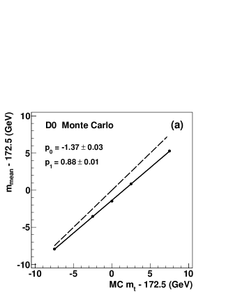
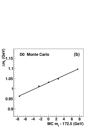
Figure 5: The response of the ME method in (a) $m_{t}$, (b) statistical uncertainty on the $m_{t}$, and (c) the pull width, shown as a function of the MC input $m_{t}$ for the combined $ee$, $e\mu$, and $\mu\mu$ channels. The error bars in (a) and (b) are invisibly small. The dashed line in (a) represents the case of ideal response.

Final state	$ee$	$e\mu$	$\mu\mu$	$\ell\ell$
Uncertainty, GeV	3.69	1.71	3.57	1.45

Table 3: The expected statistical uncertainties for a generated $m_{t}=172.5$ GeV for the $ee$, $e\mu$, and $\mu\mu$ channels and their combination.

The expected statistical uncertainty for the generated top quark mass of 172.5 GeV is calculated as $\Delta m_{t}^{\rm exp}=\Delta m_{t}(172.5\ {\rm GeV})\cdot w_{\rm pull}/p_{1}$, and given in Table 3.

IV Fit to Data

The fit to data is first performed using an unknown random offset in the measured mass. This offset is removed only after the final validation of the methodology. We apply the ME technique to data as follows:

1. The $k_{\rm JES}$  correction factor from the lepton+jets mass analysis Abazov et al. (2014a, 2015) is applied to the jet $p_{T}$ in data as $p^{\rm corr}_{T}=p_{T}/k_{\rm JES}$ (Section II). The uncertainties related to the propagation of this correction from $\ell$+jets to the dilepton final state are included in the systematic uncertainties as a residual JES uncertainty and statistical uncertainty on $k_{\rm JES}$ scale factor discussed in Section V.2.

2. The calibration correction from Fig. 5 is applied to $m_{\rm lhood}$ and $\sigma_{\rm lhood}$ to obtain the measured values:

   $$m_{\rm meas} =(m_{\rm lhood}-p_{0}-172.5)/p_{1}+172.5~{}{\rm(GeV)},$$ (5)

   $$\sigma_{\rm meas} =\sigma_{\rm lhood}\cdot w_{\rm pull}/p_{1}.$$

3. The fit to the log-likelihood function is the best fit to a parabola in an interval containing a 10 GeV range in MC $m_{t}$ around the minimum before its calibration.

The log-likelihood function in data is shown in Fig. 7. Table 4 shows the results for each channel separately and for their combination. The distribution in the expected statistical uncertainty for an input MC top quark mass of 175 GeV (the closest input value to the mass obtained in data) for the three combined channels is shown in Fig. 7.

Final state	Mass (GeV)
$ee$	176.94 $\pm$ 4.65
$e\mu$	172.18 $\pm$ 1.95
$\mu\mu$	176.04 $\pm$ 4.82
$\ell\ell$	$173.93$ $\pm$ $1.61$

Table 4: The calibrated top quark mass for the $ee$, $e\mu$, and $\mu\mu$ channels, and for their combination. The quoted uncertainties are statistical.

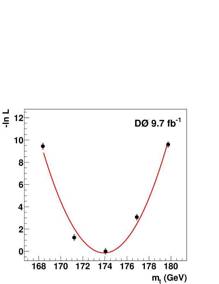
Figure 6: The negative log-likelihood ratio for the combined $ee$, $e\mu$, and $\mu\mu$ data after calibration, as a function of the input MC $m_{t}$. The curve is the best fit to a parabola in the interval 168.4 $-$ 179.7 GeV.

Figure 7: The distribution in the expected statistical uncertainty $\sigma_{\rm lhood}^{\rm exp}$ for the combined $ee$, $e\mu$, and $\mu\mu$ channels after applying calibration, for the MC input $m_{t}=175$ GeV. The arrow indicates the statistical uncertainty for data after the calibration ($\sigma_{\rm meas}$).

V Systematic Uncertainties and Results

Systematic uncertainties affect the measured $m_{t}$ in two ways. First, the distribution in the signal and background log-likelihood functions can be affected directly by a change in some parameter, leading to a bias in the calibration. Second, the signal-to-background ratio in the selected data can be affected by the parameter change, leading to a difference in the combined signal and background log-likelihood function, again causing a a bias in the calibration. Ideally, these two contributions can be treated coherently for each source of systematic uncertainty, but since the second effect is much smaller than the first for the most important systematic uncertainties, we keep the same signal-to-background ratio in pseudo-experiments, except for the systematic uncertainty in the signal fraction. Background events are included in the evaluation of all sources of systematic uncertainty, and all systematic uncertainties are evaluated using the simulated events with a top quark mass of 172.5 GeV.

V.1 Systematic uncertainties in modeling signal and background

We determine uncertainties related to signal modeling by comparing simulations with different generators and parameters, as described below.

Higher order corrections. By default, we use LO alpgen to model signal events. To evaluate the effect of higher-order corrections on the top quark mass, we use signal events generated with the NLO MC generator mc@nlo (version 3.4) Frixione and Webber (2002, 2008), interfaced to herwig (version 6.510) Corcella et al. (2001) for parton showering and hadronization. The CTEQ6M PDFs Pumplin et al. (2002); Nadolsky et al. (2008) are used to generate events at a top quark mass of $m_{t}=172.5$ GeV. Because mc@nlo is interfaced to herwig for simulating the showering contributions to the process of interest, we use alpgen+herwig events for this comparison, in order to avoid double-counting an uncertainty due to a different showering model.

Initial state radiation (ISR) and final-state radiation (FSR). This systematic uncertainty is evaluated comparing the result using alpgen+pythia  by changing the factorization and renormalization scale parameters, up and down by a factor of 2, as done in Ref. Abazov et al. (2015).

Hadronization and underlying event. The systematic uncertainty due to the hadronization and the underlying event (UE) is estimated as the difference between $m_{t}$ measured using the default alpgen+pythia events and events generated using different hadronization models. We consider three alternatives: alpgen+herwig, alpgen+pythia using Perugia Tune 2011C (with color reconnection), or using Perugia Tune 2011NOCR (without color reconnection) Skands (2010). We take the largest of these differences, which is the difference relative to alpgen+herwig, as an estimate of the systematic uncertainty for choice of effects from the hadronization and the UE.

Color reconnection. We estimate the effect of the model for color reconnection (CR) by comparing the top quark mass measured with alpgen+pythia Perugia Tune 2011C (with color reconnection), and with Perugia Tune 2011NOCR (without color reconnection) Skands (2010). Our default alpgen+pythia tune does not have explicit CR modeling, so we consider Perugia2011NOCR as the default in this comparision.

Uncertainty in modeling $\bm{b}$ quark fragmentation ($\bm{b}$ quark jet modeling). Uncertainties in simulation of $b$ quark fragmentation can affect the $m_{t}$ measurement through $b$ quark jet identification or transfer functions. This is studied using the procedure described in Ref. Peters et al. (2006) by reweighting $b$ quark fragmentation to match a Bowler scheme tuned to either LEP or SLD data.

PDF uncertainties. The systematic uncertainty due to the choice of PDF is estimated by changing the 20 eigenvalues of the CTEQ6.1M PDF within their uncertainties in $t\bar{t}$  MC simulations. Ensemble tests are repeated for each of these changes and the total uncertainty is evaluated as in Ref. Abazov et al. (2015).

Transverse momentum of the $\bm{t\bar{t}}$ system. To evaluate this systematic uncertainty, we reconstruct the $t\bar{t}$ $p_{T}$ from the two leading jets, two leading leptons, and $/\kern-5.50003ptp_{T}$. The distribution in the MC events is reweighted to match that in data using a linear fit to the $p_{T}$ distribution of the $t\bar{t}$  system. To improve statistics, we combine all the dilepton channels for the extraction of the reweighting function.

Heavy-flavor scale factor. In the alpgen $(\mbox{$Z/\gamma^{\star}$}\rightarrow\ell\ell)+\rm jets$ background samples, the fraction of heavy-flavor events is not well modelled. Therefore, a heavy-flavor scale factor is applied to the $(Z\to\ell\ell)+b\bar{b}$ and $(\mbox{$Z/\gamma^{\star}$}\to\ell\ell)+c\bar{c}$ cross sections to increase the heavy-flavor content. This scale factor has an uncertainty of $\pm 20\%$. We estimate its systematic effect by changing the scale factor within this uncertainty.

Multiple $\bm{p\bar{p}}$ interactions. Several independent $p\bar{p}$ interactions in the same bunch crossing may influence the measurement of $m_{t}$. We reweight the number of interactions in simulated MC samples to the number of interactions found in data before implementing any selection requirements. To estimate the effect from a possible mismatch in luminosity profiles, we examine the distribution in instantaneous luminosity in both data and MC after event selection, and reweight the instantaneous luminosity profile in MC events to match data.

V.2 JES systematic uncertainties

The relative difference between the JES in data and MC simulations is described by the $k_{\rm JES}$ factor extracted in the $\ell$+jets mass measurement Abazov et al. (2014a, 2015). As mentioned above, we apply this scale factor to jet $p_{T}$ in data. In the previous dilepton analysis Abazov et al. (2011b), the JES and the ratio of $b$ and light jet responses were the dominant systematic uncertainties. The improvements made in the jet calibration Abazov et al. (2014b) and use of the $k_{\rm JES}$ factor in the dilepton channel reduce the uncertainty related to the JES from 1.5 GeV to 0.5 GeV.

Residual uncertainty in JES. This uncertainty arises from the fact that the JES depends on the $p_{T}$ and $\eta$ of the jet. The JES correction in the $\ell$+jets measurement assumes a constant scale factor, i.e., we correct the average JES, but not the $p_{T}$ and $\eta$ dependence. In addition, the $k_{\rm JES}$ correction can be affected by the different jet $p_{T}$ requirements on jets in the $\ell$+jets and in dilepton final states. There can also be a different JES offset correction due to different jet multiplicities. We estimate these uncertainties as follows. We use MC events in which the jet energies are shifted upward by one standard deviation of the $\gamma$+jet JES uncertainty and correct jet $p_{T}$ in these samples to $p^{\rm corrMC}_{T}=p^{\rm MC}_{T}\cdot k^{\rm UP}_{\rm JES}/k_{\rm JES}$, where $k^{\rm UP}_{\rm JES}$ is the JES correction measured in the $\ell$+jets analysis for the MC events that are shifted up by one standard deviation. The $1/k_{\rm JES}$ factor appears because the $k_{\rm JES}$  is applied to the data and not to MC samples. Following the same approach as in Abazov et al. (2014b), we assume that the downward change for the JES samples has the same effect as the upward changes in jet $p_{T}$.

Uncertainty on the $\bm{k_{\bf{\rm JES}}}$ factor. The statistical uncertainty on the $k_{\rm JES}$  scale factor is 0.5% – 1.5% depending on the data taking period (Table 1). We recalculate the mass measured in MC with the $k_{\rm JES}$ correction shifted by one standard deviation. This procedure is applied separately for each data taking period, and the uncertainties are summed in quadrature.

Ratio of $\bm{b}$ and light jet responses or flavor-dependent uncertainty. The JES calibration used in this measurement contains a flavor-dependent jet response correction, which accounts for the difference in detector response to different jet flavors, in particular $b$ quark jets versus light-quark jets. This correction is applied to the jets in MC simulation through a convolution of the corrections for all simulated particles associated to the jet as a function of particle $p_{T}$ and $\eta$. It is constructed in a way that preserves the flavor-averaged JES corrections for $\gamma$+ jets events  Abazov et al. (2014b). The $k_{\rm JES}$ correction does not improve this calibration, because it is measured in light jet flavor from $WW\to qq^{\prime}$ decays. To propagate the effect of the uncertainty to the measured $m_{t}$ value, we change the corresponding correction by the size of the uncertainty and recalculate $m_{t}$.

V.3 Object reconstruction and identification

Trigger. To evaluate the impact of the trigger on our analysis, we scale the number of background events according to the uncertainty on the trigger efficiency for different channels. The number of signal $t\bar{t}$ events is recalculated as the difference between the number of events in data and the expected number of background events. We reconstruct ensembles according to the varied event fractions and extract the new mass.

Electron momentum scale and resolution. This uncertainty reflects the difference in the absolute lepton momentum measurement and the simulated resolution Abazov et al. (2014e) between data and MC events. We estimate this uncertainty by changing the corresponding parameters up and down by one standard deviation for the simulated samples, and assigning the difference in the measured mass as a systematic uncertainty.

Systematic uncertainty in $\bm{p_{T}}$ resolution of muons. We estimate the uncertainty by changing the muon $p_{T}$ resolution Abazov et al. (2014c) by $\pm 1$ standard deviation in the simulated samples and assign the difference in the measured mass as a systematic uncertainty.

Jet identification. Scale factors are used to correct the jet identification efficiency in MC events. We estimate the systematic uncertainty by changing these scale factors by $\pm 1$ standard deviation.

Systematic uncertainty in jet resolution. The procedure of correction of jet energies for residual differences in energy resolution and energy scale in simulated events Abazov et al. (2014b) applies additional smearing to the MC jets in order to account for the differences in jet $p_{T}$ resolution in data and MC. To compute the systematic uncertainty on the jet resolution, the parameters for jet energy smearing are changed by their uncertainties.

$\bm{b}$-tagging efficiency. A difference in $b$-tagging modeling between data and simulation may case a systematic change in $m_{t}$. To estimate this uncertainty, we change the $b$ tagging corrections up and down within their uncertainties using reweighting.

V.4 Method

MC calibration. An estimate of the statistical uncertainties from the limited size of MC samples used in the calibration procedure is obtained through the statistical uncertainty of the calibration parameters. To determine this contribution, we propagate the uncertainties on the calibration constants $p_{0}$ and $p_{1}$ (Fig. 5) to $m_{t}$.

Instrumental background. To evaluate systematic uncertainty due to instrumental background, we change its contribution by $\pm 25\%$. The number of signal $t\bar{t}$ events is recalculated by subtracting the instrumental background from the number of events in data, and ensemble studies are repeated to extract $m_{t}$.

Background contribution (or signal fraction). To propagate the uncertainty associated with the background level, we change the number of background events according to its uncertainty, rerun the ensembles, and extract $m_{t}$. In the ensembles, the number of $t\bar{t}$ events is defined by the difference in the observed number of events in data and the expected number of background events.

V.5 MC statistical uncertainty estimation

We evaluated MC statistical uncertainties in the estimation of systematic uncertainties. To obtain the MC statistical uncertainty in the $t\bar{t}$ samples, we divide each sample into independent subsets. The dispersion of masses in these subsets is used to estimate the uncertainty. The estimated MC statistical uncertainties for the signal modeling and jet and electron energy resolution are $0.11-0.14$ GeV, for all other the typical uncertainty is around $0.04$ GeV. In cases when the obtained estimate of MC statistical uncertainty is larger than the value of the systematic uncertainty, we take the MC statistical uncertainty as the systematic uncertainty.

V.6 Summary of systematic uncertainties

Table 5 summarizes all contributions to the uncertainty on the $m_{t}$ measurement with the ME method. Each source is corrected for the slope of the calibration from Fig. 5(a). The uncertainties are symmetrized in the same way as in the $\ell$+jets  measurement Abazov et al. (2014a, 2015). We use sign $\pm$ if the positive variation of the source of uncertainty corresponds to a positive variation of the measured mass, and $\mp$ if it corresponds to a negative variation for two-sided uncertainties. We quote the uncertainties for one sided sources or the ones dominated by one-side component in Table 5, indicating the direction of $m_{t}$ change when using an alternative instead of the default model. As all the entries in the total systematic uncertainty are independent, the total systematic uncertainty on the top mass measurement is obtained by adding all the contributions in quadrature.

Source	Uncertainty (GeV)
Signal and background modeling:
Higher order corrections	$+0.16$
ISR/FSR	$\pm 0.16$
Hadronization and UE	$+0.31$
Color Reconnection	$+0.15$
b-jet modelling	$+0.21$
PDF uncertainty	$\pm 0.20$
Heavy flavor	$\mp 0.06$
$p_{T}(t\bar{t})$	$+0.03$
Multiple $p\bar{p}$ interactions	$-0.10$
Detector modeling:
Residual jet energy scale	$-0.20$
Uncertainty on $k_{\rm JES}$ factor	$\mp 0.46$
Flavor dependent jet response	$\mp 0.30$
Jet energy resolution	$\mp 0.15$
Electron momentum scale	$\mp 0.10$
Electron resolution	$\mp 0.16$
Muon resolution	$\mp 0.10$
b-tagging efficiency	$\mp 0.28$
Trigger	$\pm 0.06$
Jet ID	$+0.08$
Method:
MC calibration	$\pm 0.03$
Instrumental background	$\pm 0.07$
MC background	$\pm 0.06$
Total systematic uncertainty	$\pm 0.88$
Total statistical uncertainty	$\pm 1.61$
Total uncertainty	$\pm 1.84$

Table 5: Systematic and statistical uncertainties for the measurement of $m_{t}$ in dilepton final states. The values are given for the combination of the $ee$, $e\mu$, and $\mu\mu$ channels.

VI Conclusion

We have performed a measurement of the top quark mass in the dilepton channel $t\bar{t}\to W^{+}b\ W^{-}\bar{b}\to\ell^{+}\nu_{\ell}b\ \ell^{-}\bar{\nu_{\ell}}\bar{b}$  using the matrix element technique in 9.7 fb^-1  of integrated luminosity collected by the D0 detector at the Fermilab Tevatron $p\bar{p}$ Collider. The result $m_{t}=173.93\pm 1.61\ {\rm(stat)}\pm 0.88\ {\rm(syst)}$ $\mathrm{Ge\kern-1.00006ptV}$, corresponding to a relative precision of 1.0%, is consistent with the values of the current Tevatron CDF and D0 collaborations (2014) and world combinations ATLAS Collaboration, CDF Collaboration, CMS Collaboration, and D0 Collaboration (2014).

We thank the staffs at Fermilab and collaborating institutions, and acknowledge support from the Department of Energy and National Science Foundation (United States of America); Alternative Energies and Atomic Energy Commission and National Center for Scientific Research/National Institute of Nuclear and Particle Physics (France); Ministry of Education and Science of the Russian Federation, National Research Center “Kurchatov Institute” of the Russian Federation, and Russian Foundation for Basic Research (Russia); National Council for the Development of Science and Technology and Carlos Chagas Filho Foundation for the Support of Research in the State of Rio de Janeiro (Brazil); Department of Atomic Energy and Department of Science and Technology (India); Administrative Department of Science, Technology and Innovation (Colombia); National Council of Science and Technology (Mexico); National Research Foundation of Korea (Korea); Foundation for Fundamental Research on Matter (The Netherlands); Science and Technology Facilities Council and The Royal Society (United Kingdom); Ministry of Education, Youth and Sports (Czech Republic); Bundesministerium für Bildung und Forschung (Federal Ministry of Education and Research) and Deutsche Forschungsgemeinschaft (German Research Foundation) (Germany); Science Foundation Ireland (Ireland); Swedish Research Council (Sweden); China Academy of Sciences and National Natural Science Foundation of China (China); and Ministry of Education and Science of Ukraine (Ukraine).

References

- Abazov et al. (2014a) V. M. Abazov et al. (D0 Collaboration), Precision measurement of the top-quark mass in lepton+jets final states, Phys. Rev. Lett. 113, 032002 (2014a).
- Abazov et al. (2015) V. M. Abazov et al. (D0 Collaboration), Precision measurement of the top-quark mass in leptonjets final states, Phys. Rev. D 91, 112003 (2015).
- ATLAS Collaboration, CDF Collaboration, CMS Collaboration, and D0 Collaboration (2014) ATLAS Collaboration, CDF Collaboration, CMS Collaboration, and D0 Collaboration, First combination of Tevatron and LHC measurements of the top-quark mass (2014), eprint arXiv:1403.4427.
- Khachatryan et al. (2016) V. Khachatryan et al. (CMS Collaboration), Measurement of the top quark mass using proton-proton data at and 8 TeV, Phys. Rev. D93, 072004 (2016).
- CDF and D0 collaborations (2014) CDF and D0 collaborations (CDF Collaboration, D0 Collaboration), Combination of CDF and D0 results on the mass of the top quark using up to 9.7 fb-1 at the Tevatron (2014), eprint arXiv:1407.2682.
- Abachi et al. (1995) S. Abachi et al. (D0 Collaboration), Observation of the top quark, Phys. Rev. Lett. 74, 2632 (1995).
- Abe et al. (1995) F. Abe et al. (CDF Collaboration), Observation of top quark production in collisions, Phys. Rev. Lett. 74, 2626 (1995).
- Jezabek and Kühn (1988) M. Jezabek and J. H. Kühn, Semileptonic Decays of Top Quarks, Phys. Lett. B 207, 91 (1988).
- Jezabek and Kühn (1989) M. Jezabek and J. H. Kühn, QCD Corrections to Semileptonic Decays of Heavy Quarks, Nucl. Phys. 314, 1 (1989).
- Abazov et al. (2012a) V. M. Abazov et al. (D0 Collaboration), An Improved determination of the width of the top quark, Phys. Rev. D 85, 091104 (2012a).
- Bernreuther et al. (2004) W. Bernreuther, A. Brandenburg, Z. G. Si, and P. Uwer, Top quark pair production and decay at hadron colliders, Nucl. Phys. 690, 81 (2004).
- Czakon et al. (2013) M. Czakon, M. L. Mangano, A. Mitov, and J. Rojo, Constraints on the gluon PDF from top quark pair production at hadron colliders, J. High Energy Phys. 1307, 167 (2013).
- Abazov et al. (2004) V. M. Abazov et al. (D0 Collaboration), A precision measurement of the mass of the top quark, Nature 429, 638 (2004).
- Abazov et al. (2014b) V. M. Abazov et al. (D0 Collaboration), Jet energy scale determination in the D0 experiment, Nucl. Instrum. Meth. A 763, 442 (2014b).
- Abazov et al. (2016) V. M. Abazov et al. (D0 Collaboration), Precise measurement of the top quark mass in dilepton decays using optimized neutrino weighting, Phys. Lett. B752, 18 (2016).
- Abazov et al. (2006) V. M. Abazov et al. (D0 Collaboration), The upgraded D0 detector, Nucl. Instrum. Meth. A 565, 463 (2006).
- Abazov et al. (2005) V. M. Abazov et al., The muon system of the run II D0 detector, Nucl. Instrum. Meth. A 552, 372 (2005).
- Abolins et al. (2008) M. Abolins et al., Design and Implementation of the New D0 Level-1 Calorimeter Trigger, Nucl. Instrum. Meth. A 584, 75 (2008).
- Angstadt et al. (2010) R. Angstadt et al. (D0 Collaboration), The Layer 0 Inner Silicon Detector of the D0 Experiment, Nucl. Instrum. Meth. A 622, 298 (2010).
- Ahmed et al. (2011) S. Ahmed et al. (D0 Collaboration), The D0 Silicon Microstrip Tracker, Nucl. Instrum. Meth. A 634, 8 (2011).
- Casey et al. (2013) B. Casey et al., The D0 Run IIb Luminosity Measurement, Nucl. Instrum. Meth. A 698, 208 (2013).
- Bezzubov et al. (2014) V. Bezzubov et al., The Performance and Long Term Stability of the D0 Run II Forward Muon Scintillation Counters, Nucl. Instrum. Meth. A 753, 105 (2014).
- Abazov et al. (2014c) V. M. Abazov et al. (D0 Collaboration), Muon reconstruction and identification with the Run II D0 detector, Nucl. Instrum. Meth. A 737, 281 (2014c).
- Blazey et al. (2000) G. C. Blazey et al., in Proceedings of the Workshop on QCD and Weak Boson Physics in Run II, edited by U. Baur, R. K. Ellis, and D. Zeppenfeld (2000), pp. 47–77, eprint hep-ex/0005012.
- Abazov et al. (2012b) V. M. Abazov et al. (D0 Collaboration), Measurement of the top quark mass in collisions using events with two leptons, Phys. Rev. D 86, 051103 (2012b).
- Abazov et al. (2010) V. M. Abazov et al. (D0 Collaboration), -Jet Identification in the D0 Experiment, Nucl. Instrum. Meth. A 620, 490 (2010).
- Abazov et al. (2014d) V. M. Abazov et al. (D0 Collaboration), Improved quark jet identification at the D0 experiment, Nucl. Instrum. Meth. A 763, 290 (2014d).
- Abazov et al. (2011a) V. M. Abazov et al. (D0 Collaboration), Measurement of the production cross section using dilepton events in collisions, Phys. Lett. B 704, 403 (2011a).
- Mangano et al. (2003) M. L. Mangano, M. Moretti, F. Piccinini, R. Pittau, and A. D. Polosa, ALPGEN, a generator for hard multiparton processes in hadronic collisions, J. High Energy Phys. 07, 001 (2003).
- Sjöstrand et al. (2006) T. Sjöstrand, S. Mrenna, and P. Z. Skands, PYTHIA 6.4 Physics and Manual, J. High Energy Phys. 05, 026 (2006).
- Affolder et al. (2002) T. Affolder et al. (CDF Collaboration), Charged jet evolution and the underlying event in collisions at 1.8 TeV, Phys. Rev. D 65, 092002 (2002).
- Pumplin et al. (2002) J. Pumplin et al., New generation of parton distributions with uncertainties from global QCD analysis, J. High Energy Phys. 07, 012 (2002).
- Nadolsky et al. (2008) P. M. Nadolsky et al., Implications of CTEQ global analysis for collider observables, Phys. Rev. D 78, 013004 (2008).
- Czakon and Mitov (2014) M. Czakon and A. Mitov, Top++: A Program for the Calculation of the Top-Pair Cross-Section at Hadron Colliders, Comput. Phys. Commun. 185, 2930 (2014).
- Ellis (2006) R. K. Ellis, An update on the next-to-leading order Monte Carlo MCFM, Nucl. Phys. Proc. Suppl. 160, 170 (2006).
- Brun and Carminati (1993) R. Brun and F. Carminati, Geant: Detector description and simulation tool, CERN Program Library Long Writeup W5013 (1993).
- Abazov et al. (2007) V. M. Abazov et al. (D0 Collaboration), Measurement of the production cross section in collisions at = 1.96-TeV using kinematic characteristics of lepton + jets events, Phys. Rev. D76, 092007 (2007).
- Abazov et al. (2013) V. M. Abazov et al. (D0 Collaboration), Measurement of the asymmetry in angular distributions of leptons produced in dilepton final states in collisions at = 1.96 TeV, Phys. Rev. D 88, 112002 (2013).
- Abazov et al. (2011b) V. M. Abazov et al. (D0 Collaboration), Precise measurement of the top quark mass in the dilepton channel at D0, Phys. Rev. Lett. 107, 082004 (2011b).
- Mahlon and Parke (1997) G. Mahlon and S. J. Parke, Maximizing spin correlations in top quark pair production at the Tevatron, Phys. Lett. B 411, 173 (1997).
- Fiedler et al. (2010) F. Fiedler, A. Grohsjean, P. Haefner, and P. Schieferdecker, The Matrix Element Method and its Application in Measurements of the Top Quark Mass, Nucl. Instrum. Meth. A 624, 203 (2010).
- Lepage (1978) G. Lepage, A new algorithm for adaptive multidimensional integration, Journal of Computational Physics 27, 192 (1978).
- Lepage (1980) G. Lepage, VEGAS: An Adaptive Multi-dimensional Integration Program (1980), Cornell preprint CLNS 80-447.
- Galassi et al. (2009) M. Galassi, J. Davies, J. Theiler, B. Gough, G. Jungman, P. Alken, M. Booth, and F. Rossi, GNU Scientific Library Reference Manual - Third Edition, ISBN 0954612078 (Network Theory Ltd, 2009).
- Berends et al. (1991) F. A. Berends, H. Kuijf, B. Tausk, and W. T. Giele, On the production of a W and jets at hadron colliders, Nucl. Phys. B357, 32 (1991).
- Grohsjean (2008) A. Grohsjean, Measurement of the top quark mass in the dilepton final state using the matrix element method (2008), Fermilab-Thesis-2008-92.
- Frixione and Webber (2002) S. Frixione and B. R. Webber, Matching NLO QCD computations and parton shower simulations, J. High Energy Phys. 06, 029 (2002).
- Frixione and Webber (2008) S. Frixione and B. R. Webber, The MC@NLO 3.4 Event Generator (2008), eprint arXiv:0812.0770.
- Corcella et al. (2001) G. Corcella et al., HERWIG 6.5: an event generator for Hadron Emission Reactions With Interfering Gluons (including supersymmetric processes), J. High Energy Phys. 01, 010 (2001).
- Skands (2010) P. Z. Skands, Tuning Monte Carlo Generators: The Perugia Tunes, Phys. Rev. D 82, 074018 (2010).
- Peters et al. (2006) Y. Peters, K. Hamacher, and D. Wicke, Precise tuning of the b fragmentation for the D0 Monte Carlo, FERMILAB-TM-2425-E (2006).
- Abazov et al. (2014e) V. M. Abazov et al. (D0 Collaboration), Electron and Photon Identification in the D0 Experiment, Nucl. Instrum. Meth. A 750, 78 (2014e).