Landau quantization, Aharonov-Bohm effect and two-dimensional pseudoharmonic quantum dot around a screw dislocation

Abstract

In this paper, we investigate the influence of a screw dislocation on the energy levels and the wavefunctions of an electron confined in a two-dimensional pseudoharmonic quantum dot under the influence of an external magnetic field inside a dot and Aharonov-Bohm field inside a pseudodot. The exact solutions for energy eigenvalues and wavefunctions are computed as functions of applied uniform magnetic field strength, Aharonov-Bohm flux, magnetic quantum number and the parameter characterizing the screw dislocation, the Burgers vector. We investigate the modifications due to the screw dislocation on the light interband absorption coefficient and absorption threshold frequency. Two scenarios are possible, depending on if singular effects either manifest or not. We found that as the Burgers vector increases, the curves of frequency are pushed up towards of the growth of it. One interesting aspect which we have observed is that the Aharonov-Bohm flux can be tuned in order to cancel the screw effect of the model.

I Introduction

The study of quantum dynamics for particles in constant magnetic Landau and Lifschitz (1981) and Aharonov-Bohm (AB) flux fields Aharonov and Bohm (1959), which are perpendicular to the plane where the particles are confined, has been carried out over the last years. The existence of other potentials are also included, depending on the purpose of the investigation. For example, in Ref. Tan and Inkson (1996) an exactly soluble model to describe quantum dots, anti-dots, one-dimensional rings and straight two-dimensional wires in the presence of such fields was proposed. It is an ideal tool to investigate the AB effects and the persistent currents in quantum rings, for instance. In Ikhdair and Sever (2007), the exact bound-state energy eigenvalues and the corresponding eigenfunctions for several diatomic molecular systems in a pseudoharmonic potential were analytically calculated for any arbitrary angular momentum. The Dirac bound states of anharmonic oscillator Hamzavi et al. (2014) and the nonrelativistic molecular models Ikhdair et al. (2015) under external magnetic and AB flux fields were investigated recently. Other examples can be found elsewhere.

On the other hand, the investigation on how a screw dislocation affects quantum phenomena in semiconductors has received considerable attention. In the continuum limit (low energy), such works are based on the geometric theory of defects in semiconductors developed by Katanaev and Volovich Katanaev and Volovich (1992). In this approach, the semiconductor with a screw dislocation is described by a Riemann-Cartan manifold where the torsion is associated to the Burgers vector. In this continuum limit, a screw dislocation affects a quantum system like an isolated magnetic flux tube, causing an AB interference phenomena Kawamura (1978); Bueno et al. (2016). The energy spectrum of electrons around this kind of defect shows a profile similar to that of the AB system Bausch et al. (1999a, 1998); Furtado and Moraes (1999); Bakke and Moraes (2012); Lorenci and Jr. (2012); Netto et al. (2008). These works describe the effect due to the geometric electron motion only. A second ingredient plays an important role in these quantum systems. It is an additional deformed potential induce by a lattice distortion Bausch et al. (1999b). It is a repulsive scalar potential(noncovariant) and shows pronounced influences in the physical quantities in such systems. The impact of this potential was first addressed in Ref. Bausch et al. (1999a), where the scattering of electrons around a screw dislocation was investigated. Recently, it was showed that a single screw dislocation has profound influences on the electronic transport in semiconductors Taira and Shima (2014). Both contributions, the covariant and noncovariant terms, were taken into account. For the electronic device industry, these defects represents a problem since they interfere in the electronic properties of the materials by way of scattering, due to such repulsive potential. Therefore, research on screw dislocation and how it may influence the dynamics of carriers is important for the improvement of electronic technology, the discovery of new phenomena and better control of transmission processesSlager et al. (2014, 2016).

In this paper, we investigate how the quantum dots and antidots, with the pseudoharmonic interaction and under the influence of external magnetic and AB flux fields, are influenced by the presence of a screw dislocation. We obtain exact analytical expressions for the energy spectrum and wavefunctions. The modification due such topological defect in the light absorption coefficient is examined and its influences in the threshold frequency value of absorption coefficient are addressed. Two scenarios are possible, depending on if singular effects are taking into account or are not. It is found that when the Burgers increases, the curves of such frequency are pushed up towards its growth. It is also noted that the AB flux can be tuned in order to cancel the influence of the screw dislocation in those physical quantities.

The plan of this work is the following. In Sec. II, we derive the Schrodinger equation for an electron around a screw dislocation in the presence of an external magnetic field, an AB field and in the presence of a two-dimensional pseudoharmonic potential. This case can find applications in the context of quantum dots and anti-dots. In Sec. III, we investigate how the screw dislocation affects such energy levels and we investigate the impact on them due to the deformed potential. We consider the electron confined on an interface so that we can discus our results in the context of a (quasi) two dimensional electron gas (2DEG). In Sec. IV, we investigate the modifications due to the screw dislocation on the light interband absorption coefficient and absorption threshold frequency. The conclusions remarks are outlined in Section V.

II The Schrodinger equation for an electron around a screw dislocation

Consider the model consisting of a non interacting electron gas around an infinitely long linear screw dislocation oriented along the $z$-axis. The three-dimensional geometry of this medium is characterized by a torsion which is identified with the surface density of the Burgers vector in the classical theory of elasticity. In order to understand the dynamics of this system in a more consistent manner, we must take into account the existence of a deformed potential, which is induced by elastic deformations on the 3D crystal. The metric of the medium with this kind of defect is given (in cylindrical coordinates) by Katanaev and Volovich (1992)

$$ds^{2}=\left(dz+\beta d\varphi\right)^{2}+d\rho^{2}+\rho^{2}d\varphi^{2},$$ (1)

with $\left(\rho,\varphi,z\right)\rightarrow\left(\rho,\varphi+2\pi,z\right)$ and $\beta$ is a parameter related to the Burgers vector $b$ by $\beta=b/2\pi$. The induced metric describes a flat medium with a singularity at the origin. The only non-zero component of the torsion tensor is given by the two form

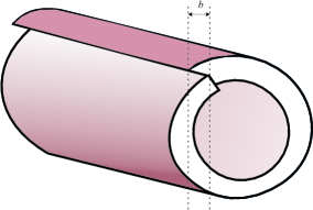
Figure 1: Cylindrical portion of a 3D solid showing the dislocation.

$$T^{1}=2\pi\beta\delta^{2}(\rho)d\rho\wedge d\varphi,$$ (2)

with $\delta^{2}(\rho)$ being the two-dimensional delta function in the flat space. Figure 1 illustrates the formation of a screw dislocation in the bulk of a 3D crystal.

Since we consider electrons on common semiconductors, we have to introduce a deformed potential which describes the effects of the lattice deformation on the electronic properties in such materials Bausch et al. (1999b). For a screw dislocation, it is found to be

$$V_{d}(\rho)=\frac{\hbar^{2}}{2ma^{2}}\frac{b^{2}}{4\pi^{2}\rho^{2}}\left[2+a^{2}\left(\frac{\partial}{\partial z}\right)^{2}\right],$$ (3)

where $a$ is the lattice constant.

The Hamiltonian for a quantum charged particle in a background $g_{ij}$ in the presence of the potential described above and in the presence of magnetic fields is given by

$$H=\frac{1}{2m}\left(p_{i}-eA_{i}\right)g^{ij}\left(p_{j}-eA_{j}\right)+V_{d}(\rho),$$ (4)

where $g\equiv\det{g_{ij}}$, with $i,j=\rho,\varphi,z$ and $e$ is the electric charge. For the field configuration, we consider the existence of a constant magnetic field along the $z$-direction, $\mathbf{B_{1}}=B\mathbf{\hat{z}}$, which is obtained from the potential (in the Landau gauge),

$$\mathbf{A}_{1}=\frac{B\rho}{2}\mathbf{\hat{\varphi}}.$$ (5)

We also consider in the model the presence of the AB potential,

$$\mathbf{A}_{2}=\frac{\phi_{AB}}{2\pi\rho}\mathbf{\hat{\varphi}},$$ (6)

which provides the magnetic flux tube

$$\mathbf{B_{2}}=\frac{\phi_{AB}}{2\pi}\frac{\delta(\rho)}{\rho}\mathbf{\hat{z}},$$ (7)

and a scalar pseudoharmonic interaction defined by

$$V_{\mathrm{conf}}=V_{0}\left(\frac{\rho}{\rho_{0}}-\frac{\rho_{0}}{\rho}\right)^{2},$$ (8)

where $\rho_{0}$ and $V_{0}$ are the zero point (effective radius) and the chemical potential Ikhdair and Hamzavi (2012). As pointed out in Ref. Taira and Shima (2014), the presence of a screw dislocation causes an effective vector potential $\mathbf{A}_{\mathrm{eff}}$ defined by

$$\mathbf{A}_{\mathrm{eff}}\equiv\mathbf{\hat{\varphi}}\frac{\hbar b}{2\pi\rho}\frac{\partial}{\partial z}.$$ (9)

The magnitude of screw dislocation, $b$, plays a similar role to $\phi_{AB}$ in the AB system, but $\mathbf{A}_{\mathrm{eff}}$ is a differential operator instead.

Our goal is to solve the problem of an electron gas interacting with $\mathbf{A}_{1}+\mathbf{A}_{2}+\mathbf{A}_{\mathrm{eff}}$. This model is described by the Schr dinger equation

$$-\frac{\hbar^{2}}{2m}\left[\frac{\partial^{2}}{\partial z^{2}}+\frac{\partial^{2}}{\partial\rho^{2}}+\frac{1}{\rho}\frac{\partial}{\partial\rho}+\frac{1}{\rho^{2}}\left(\frac{\partial}{\partial\varphi}-\beta\frac{\partial}{\partial z}+\delta\right)^{2}\right]\psi$$

$$+\left[\frac{ieB\hbar}{2m}\left(\frac{\partial}{\partial\varphi}-\beta\frac{\partial}{\partial z}+\delta\right)+\frac{e^{2}B^{2}\rho^{2}}{8m}\right]\psi$$

$$+V_{d}(\rho)\psi+V_{\mathrm{conf}}(\rho)\psi=E\psi,$$ (10)

where $\delta\equiv e\phi_{AB}/2\pi\hbar$ is the flux parameter.

In the next section, we solve the Schrodinger equation above and discuss the impact of such deformed potential on the energy levels around this kind of defect.

III Influence of a screw dislocation on the energy levels

In this section, we start by investigating the influence of the screw dislocation on the energy levels of electrons on a 3D solid taking into account the deformed potential (3). The equation (10) is solved by considering the ansatz $\psi(\rho,\varphi,z)=Ce^{il\varphi}e^{ik_{z}z}R(\rho)$, where $l=0,\pm 1,\pm 2,\pm 3,...$, $k_{z}\in\Re$ and $C$ is a normalization constant. Equation (10) leads to

$$-\frac{\hbar^{2}}{2m}\left[\frac{d^{2}}{d\rho^{2}}+\frac{1}{\rho}\frac{d}{d\rho}-\frac{1}{\rho^{2}}\left(l-\beta k+\delta\right)^{2}-k^{2}\right]R(\rho)$$

$$+\left[\frac{e^{2}B^{2}\rho^{2}}{8m}-\frac{eB\hbar}{2m}\left(l-\beta k+\delta\right)+V_{0}\left(\frac{\rho}{\rho_{0}}-\frac{\rho_{0}}{\rho}\right)^{2}\right]R(\rho)$$

$$+\frac{\hbar^{2}}{2ma^{2}}\frac{b^{2}}{4\pi^{2}\rho^{2}}\left(2+a^{2}k^{2}\right)R(\rho)=ER(\rho).$$ (11)

This differential equation can be rewritten as

$$\left[\frac{d^{2}}{d\rho^{2}}+\frac{1}{\rho}\frac{d}{d\rho}-\frac{\nu^{2}}{\rho^{2}}-\Omega^{2}\rho^{2}+\epsilon\right]R(\rho)=0,$$ (12)

where

$$\epsilon=\frac{2m}{\hbar^{2}}\left[E-k^{2}+\frac{eB\hbar}{2m}\left(l-\beta k+\delta\right)+2V_{0}\right],$$

$$\nu^{2}=\left(l-\beta k+\delta\right)^{2}+\frac{2\beta^{2}}{a^{2}}\left(1-\frac{k^{2}a^{2}}{2}\right)+\frac{2mV_{0}\rho_{0}^{2}}{\hbar^{2}},$$

and

$$\Omega^{2}=\frac{e^{2}B^{2}}{4\hbar^{2}}+\frac{2mV_{0}}{\hbar^{2}\rho_{0}^{2}}.$$

The general solution of the eigenvalue equation (12) is given by Abramowitz and Stegun (1972)

$$R(\rho) =C_{1}e^{-\frac{\Omega}{2}\rho^{2}}(\Omega\rho^{2})^{\frac{1}{2}+\frac{\left|\nu\right|}{2}}\mathrm{M}\left(d_{\nu},1+\left|\nu\right|,\Omega\rho^{2}\right)$$

$$+C_{2}e^{-\frac{\Omega}{2}\rho^{2}}(\Omega\rho^{2})^{\frac{1}{2}+\frac{\left|\nu\right|}{2}}\mathrm{U}\left(d_{\nu},1+\left|\nu\right|,\Omega\rho^{2}\right),$$ (13)

with

$$d_{\nu}=\frac{1}{2}+\frac{\left|\nu\right|}{2}-\frac{\epsilon}{4\Omega}.$$ (14)

The functions $\mathrm{M}$ and $\mathrm{U}$ in Eq. (13) denote the confluent hypergeometric functions of the first and second kind, respectively. Unlike $\mathrm{M}(a,b,z)$, which is an entire function of $z$, $U(a,b,z)$ may show a singularity at zero. If our system does not show singularity, then we can make $C_{2}\equiv 0$. However, if the wavefunction couples with singular potentials, we can instead, make $C_{1}\equiv 0$ Hagen (2008). Remember that our electron gas is in a region where exist a topological defect, which may introduce a singularity in our problem. We first consider the case for regular wavefunctions and after that we discuss what changes whenever we have the irregular ones. Therefore, we are left with

$$R(\rho)=C_{1}e^{-\frac{\Omega}{2}\rho^{2}}(\Omega\rho^{2})^{\frac{1}{2}+\frac{\left|\nu\right|}{2}}\mathrm{M}\left(d_{\nu},1+\left|\nu\right|,\Omega\rho^{2}\right).$$ (15)

A necessary condition for $R(\rho)$ to be square-integrable is $\lim_{\rho\rightarrow\infty}R(\rho)=0$, which is fulfilled if $d_{\nu}=-n$, with $n=0,1,2,3,...$. In this way, the eigenvalues of Eq. (12) are given by

$$E_{n}=\left(2n+\left|\nu\right|+1\right)\frac{\Omega\hbar^{2}}{m}-\left(l-\beta k+\delta\right)\frac{\hbar\omega_{c}}{2}+\frac{\hbar^{2}k^{2}}{2m}-2V_{0},$$ (16)

where $\omega_{c}\equiv eB/m$ is the cyclotron frequency. Equation (16) are the modified Landau levels. For $\delta=0$ and $V_{0}=0$, we have

$$E_{n}\equiv E_{n}^{\mathrm{deff}}=\left(n+\frac{\left|\nu\right|}{2}-\frac{l-\beta k}{2}+\frac{1}{2}\right)\hbar\omega_{c}+\frac{\hbar^{2}k^{2}}{2m}.$$ (17)

Notice that the deformed potential has a pronounced influence on the energy levels. In the absence of such interaction, the energy levels are given by Furtado and Moraes (1999)

$$E_{n}=\left(n+\frac{\left|l-\beta k\right|}{2}-\frac{l-\beta k}{2}+\frac{1}{2}\right)\hbar\omega_{c}+\frac{\hbar^{2}k^{2}}{2m}.$$ (18)

For $\delta=0$, $V_{0}=0$, $\beta=0$ and ignoring the motion along the $z-$ direction, we have

$$E_{n}=\left(n+\frac{1}{2}\right)\hbar\omega_{c}\;,$$

which are the usual Landau levels for electrons on a flat sample.

At this point, we consider the electrons on an flat interface, with thickness $d$, around a screw dislocation. They are confined by an infinite square well potential in the $z$-direction ($0\leq z\leq d$). This way, we have $k_{z}=\ell\pi/d$ , where $\ell=1,2,3,...$ We will consider just the first transverse mode $\ell=1$ filled. Then, the parameter $\nu^{2}$ in Eq. (12) can be put in the following way,

$$\nu^{2}=\left(l-\frac{b}{2d}+\delta\right)^{2}+\frac{b^{2}}{2a^{2}\pi^{2}}-\frac{1}{4}\frac{b^{2}}{d^{2}}+\frac{2mV_{0}\rho_{0}^{2}}{\hbar^{2}}.$$ (19)

In the case where $\delta\equiv 0$ and $V_{0}\equiv 0$, we have

$$\nu^{2}=\left(l-\frac{b}{2d}\right)^{2}+\frac{b^{2}}{2a^{2}\pi^{2}}-\left(\frac{b}{2d}\right)^{2}.$$ (20)

As pointed out above, the presence of a deformed potential has a pronounced influence on the energy levels, since in its absence, we have just

$$\nu=\left(l-\frac{a}{2d}\right).$$ (21)

In the absence of both the magnetic fields, we find

$$E_{n}=\hbar\sqrt{\frac{8V_{0}}{m\rho_{0}^{2}}}\left(n+\frac{1}{2}+\frac{\left|\mu\right|}{2}\right)+\frac{\hbar^{2}k^{2}}{2m}-2V_{0},$$ (22)

where

$$\mu^{2}=\left(l-\frac{b}{2d}\right)^{2}+\frac{b^{2}}{2a^{2}\pi^{2}}-\frac{b^{2}}{4d^{2}}+\frac{2mV_{0}\rho_{0}^{2}}{\hbar^{2}}.$$

In the absence of the deformed potential, we have

$$\mu^{2}=\left(l-\frac{b}{2d}\right)^{2}+\frac{2mV_{0}\rho_{0}^{2}}{\hbar^{2}}.$$ (23)

We now turn our attention to the case considering the irregular solution which is achieved by considering $C_{1}\equiv 0$ in Eq. (13), that is

$$R(\rho)=C_{1}e^{-\frac{\Omega}{2}\rho^{2}}\left(\Omega\rho^{2}\right)^{\frac{1}{2}+\frac{\left|\nu\right|}{2}}\mathrm{U}\left(-n,1+\left|\nu\right|,\Omega\rho^{2}\right).$$ (24)

As showed in Ref. Filgueiras et al. (2010), this solution diverges as $\rho\rightarrow 0$ but is square integrable when

$$-1<\left|\nu\right|<1\;.$$ (25)

The eigenvalue of (24) are the same given by Eq. (16) but with the constraint (25) above, which can be achieved only if $l=0$. In Eq. (16), any value of $l$ is allowed.

IV Influence of the screw dislocation on the interband light absorption coefficient and in the threshold frequency value of absorption

In this section, we calculate the direct interband light absorption coefficient $K(\omega)$ and the threshold frequency of absorption in a quantum pseudodot under the influence of external magnetic field, AB flux field and the screw dislocation. The light absorption coefficient can be expressed asAtoyan et al. (2004, 2006); Raigoza et al. (2005); Khordad (2010)

$$K(\omega) =N$$

$$\times\sum_{n,l,\nu}\sum_{n^{\prime},l^{\prime},\nu^{\prime}}\left|\int\psi_{n,m,\nu}^{e}\left(\rho,\phi\right)\psi_{n^{\prime},l^{\prime},\nu^{\prime}}^{h}\left(\rho,\phi\right)\rho d\rho d\phi\right|^{2}$$

$$\times\delta\left(\Delta-E_{n,m,\nu}^{e}-E_{n^{\prime},l^{\prime},\nu^{\prime}}^{h}\right),$$ (26)

where $\Delta\equiv\hbar\varpi-\varepsilon_{g}$, $\varepsilon_{g}$ is the width of forbidden energy gap, $\varpi$ is the frequency of incident light, $N$ is a quantity proportional to the square of dipole moment matrix element modulus, $\psi^{e\left(h\right)}$ is the wave function of the electron(hole) and $E^{e(h)}$ is the corresponding energy of the electron (hole). Considering the solution (15), the Eq.(26) becomes Ikhdair and Hamzavi (2012)

$$K(\omega) =N\sum_{n,l,\nu}\sum_{n^{\prime},l^{\prime},\nu^{\prime}}\frac{\Omega^{\left|\nu\right|+\left|\nu^{\prime}\right|+2}(n+\left|\nu\right|)!(n^{\prime}+\left|\nu^{\prime}\right|)!}{\pi^{2}n!n^{\prime}!\left(\left|\nu\right|!\right)^{2}(\left|\nu^{\prime}\right|!)^{2}}$$

$$\times\Bigg{|}\int_{0}^{2}\pi e^{i(l+l^{\prime})}\int_{0}^{\infty}\rho d\rho e^{-\frac{1}{2}(\Omega+\Omega^{{}^{\prime}})\rho^{2}}\rho^{\left|\nu\right|+\left|\nu^{\prime}\right|}$$

$$\times\,\mathrm{M}\left(-n,1+\left|\nu\right|,\Omega\rho^{2}\right)\mathrm{M}\left(-n^{\prime},1+\left|\nu^{\prime}\right|,\Omega^{\prime}\rho^{2}\right)\Bigg{|}^{2}$$

$$\times\,\delta\left(\Delta-E_{n,m,\nu}^{e}-E_{n^{\prime},l^{\prime},\nu^{\prime}}^{h}\right).$$ (27)

Following Ref. Ikhdair and Hamzavi (2012), the light absorption coefficient is given by

$$K\left(\omega\right)=N\sum_{n,l,\nu}\sum_{n^{\prime},l^{\prime},\nu^{\prime}}P_{nn^{\prime}}^{\nu}Q_{nn^{\prime}}^{\nu}\delta\left(\Delta-E_{n,m,\nu}^{e}-E_{n^{\prime},l^{\prime},\nu^{\prime}}^{h}\right),$$ (28)

where

$$P_{nn^{{}^{\prime}}}^{\nu} =\frac{1}{\left(\left|\nu\right|!\right)^{4}}(\Omega\Omega^{\prime})^{\left|\nu\right|+1}\left(\frac{\Omega+\Omega^{\prime}}{\Omega-\Omega^{\prime}}\right)^{2\left(n+n^{\prime}\right)}$$

$$\times\frac{\left(n+\left|\nu\right|\right)!\left(n^{\prime}+\left|\nu\right|\right)!}{n!n^{\prime}!},$$

and

$$Q_{nn^{\prime}}^{\nu}=\left[A_{\left|\nu\right|,\Omega}\mathrm{M}\left(n,n^{\prime},\left|\nu\right|+1;-\frac{4\Omega\Omega^{\prime}}{\left(\Omega-\Omega^{\prime}\right)^{2}}\right)\right]^{2},$$

where

$$A_{\left|\nu\right|,\Omega}=\left(\left|\nu\right|\right)!\left(\frac{2}{\Omega+\omega^{\prime}}\right)^{2\left|\nu\right|+1}.$$

For the case considering the irregular solution above, we must consider the expressions above but changing the function $\mathrm{M}$(the confluent hypergeometric functions of the first kind) by $\mathrm{U}$ (the confluent hypergeometric functions of the second kind). For this last case, only $l=0$ is allowed.

From Eqs. (16) and (27), the threshold frequency of absorption will be given by

$$\hbar\varpi =\left(2n+\left|\nu\right|+1\right)\left(\frac{\Omega_{h}}{m_{h}}+\frac{\Omega_{e}}{m_{e}}\right)\hbar^{2}$$

$$-\frac{1}{2}\left(\frac{1}{m_{h}}+\frac{1}{m_{e}}\right)\left(l-\beta k+\delta\right)\hbar eB$$

$$+\frac{1}{2}\left(\frac{1}{m_{h}}+\frac{1}{m_{e}}\right)\hbar^{2}k^{2}+\varepsilon_{g}-4V_{0},$$ (29)

where $m_{e}$($m_{h}$) are the electron effective mass(hole effective mass) and

$$\Omega_{e}=\sqrt{\frac{e^{2}B^{2}}{4\hbar^{2}}+\frac{2m_{e}V_{0}}{\hbar^{2}\rho_{0}^{2}}},\;\;\Omega_{h}=\sqrt{\frac{e^{2}B^{2}}{4\hbar^{2}}+\frac{2m_{h}V_{0}}{\hbar^{2}\rho_{0}^{2}}}.$$

By ignoring the motion along $z$-direction and in the absence of both the defect($\beta\equiv 0$) and the AB flux field($\delta\equiv 0$), we recover the threshold frequency of absorption found in Ref. Khordad (2010). Further, taking $(n,l)=(0,0)$ in the presence of the fields (5) and (6), we find

$$\hbar\varpi_{00} =\left(\left|\nu_{l=0}\right|+1\right)\left(\frac{\Omega_{h}}{m_{h}}+\frac{\Omega_{e}}{m_{e}}\right)\hbar^{2}$$

$$+\frac{1}{2}\left(\frac{1}{m_{h}}-\frac{1}{m_{e}}\right)\left(\delta-\beta k\right)\hbar eB$$

$$+\varepsilon_{g}+\frac{1}{2}\left(\frac{1}{m_{h}}+\frac{1}{m_{e}}\right)\hbar^{2}k^{2}-4V_{0}.$$ (30)

In the absence of screw dislocation, we recover the expressions of Ref. Ikhdair and Hamzavi (2012), that is

$$\hbar\varpi_{00}^{b\equiv 0} =\left(1+\sqrt{\delta^{2}+\frac{2m_{h}V_{0}\rho_{0}^{2}}{\hbar^{2}}}\right)\frac{\Omega_{h}}{m_{h}}\hbar^{2}$$

$$+\left(1+\sqrt{\delta^{2}+\frac{2m_{e}V_{0}\rho_{0}^{2}}{\hbar^{2}}}\right)\frac{\Omega_{e}}{m_{e}}\hbar^{2}$$

$$+\varepsilon_{g}+\frac{1}{2}\left(\frac{1}{m_{h}}-\frac{1}{m_{e}}\right)\hbar eB\delta-4V_{0}.$$ (31)

Due to the presence of the defect, we now have the following expression for the the threshold frequency,

$$\hbar\varpi_{00}^{\mathrm{screw}} =\left(1+\sqrt{\delta^{2}-\frac{\delta b}{d}+\frac{b^{2}}{2a^{2}\pi^{2}}+\frac{2m_{e}V_{0}\rho_{0}^{2}}{\hbar^{2}}}\right)\frac{\Omega_{e}}{m_{e}}\hbar^{2}$$

$$+\left(1+\sqrt{\delta^{2}-\frac{\delta b}{d}+\frac{b^{2}}{2a^{2}\pi^{2}}+\frac{2m_{h}V_{0}\rho_{0}^{2}}{\hbar^{2}}}\right)\frac{\Omega_{h}}{m_{h}}\hbar^{2}$$

$$+\varepsilon_{g}+\frac{1}{2}\left(\frac{1}{m_{h}}-\frac{1}{m_{e}}\right)\left(\delta-\frac{b}{2d}\right)\hbar eB-4V_{0},$$ (32)

if the deformed potential is taken into account. When $\delta\equiv 0$, Eq. (32) become

$$\hbar\varpi_{00}^{\mathrm{screw}} =\left(1+\sqrt{\frac{b^{2}}{2a^{2}\pi^{2}}+\frac{2m_{e}V_{0}\rho_{0}^{2}}{\hbar^{2}}}\right)\frac{\Omega_{e}}{m_{e}}\hbar^{2}$$

$$+\left(1+\sqrt{\frac{b^{2}}{2a^{2}\pi^{2}}+\frac{2m_{h}V_{0}\rho_{0}^{2}}{\hbar^{2}}}\right)\frac{\Omega_{h}}{m_{h}}\hbar^{2}$$

$$+\varepsilon_{g}-\frac{1}{4d}\left(\frac{1}{m_{h}}-\frac{1}{m_{e}}\right)\hbar eBb-4V_{0}.$$ (33)

Let us now investigate the influence of the screw dislocation on the threshold value of absorption for transition $000\rightarrow 000$, comparing the two cases, one with and the other without the noncovariant deformed potential. The argument of Dirac delta function allows one to define such threshold value of absorption as

$$\frac{\hbar\varpi_{00}}{\varepsilon_{g}}=1+\frac{E_{0}^{e}+E_{0}^{h}}{\varepsilon_{g}}.$$

Let us now set the following parameters:

$$\eta=\frac{\rho_{0}\varepsilon_{g}}{\hbar}\sqrt{\frac{m_{e}}{V_{0}}},\;\;\eta^{\prime}=\frac{\rho_{0}\varepsilon_{g}}{\hbar}\sqrt{\frac{m_{h}}{V_{0}}},$$

$$\kappa=\frac{e\hbar B}{m_{e}\varepsilon_{g}},\;\kappa^{\prime}=\frac{e\hbar B}{m_{h}\varepsilon_{g}}.$$

For a quantum dot, we take $V_{0}\rho_{0}^{2}\rightarrow 0$. In this case, we obtain

$$\frac{E_{0}^{e}}{\varepsilon_{g}}=\frac{1}{2}(1+\xi)\sqrt{\kappa^{2}+\frac{8}{\eta^{2}}}-\frac{\kappa}{2}\left(\delta-\frac{b}{2d}\right)-\frac{2V_{0}}{\varepsilon_{g}},$$ (34)

$$\frac{E_{0}^{h}}{\varepsilon_{g}}=\frac{1}{2}(1+\xi)\sqrt{\kappa^{\prime 2}+\frac{8}{\eta^{\prime 2}}}+\frac{\kappa^{\prime}}{2}\left(\delta-\frac{b}{2d}\right)-\frac{2V_{0}}{\varepsilon_{g}},$$ (35)

where

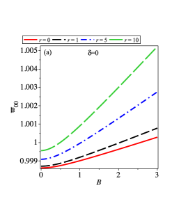
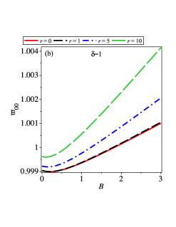
Figure 2: The variations of threshold frequency of absorption $\varpi_{00}$ (in unit of $\epsilon_{g}$) as function of $B$ for several values of the $r$ parameter. In (a) we display $\varpi_{00}$ for absence of a flux field $\delta=0$ and in (b) we display $\varpi_{00}$ for $\delta=1.0$.

$$\xi=\sqrt{\delta^{2}-\frac{\delta b}{d}+\frac{b^{2}}{2a^{2}\pi^{2}}}.$$

On the other hand, for a quantum anti-dot, we take the limit $\left(V_{0}/\rho_{0}^{2}\right)\rightarrow 0$. In this case, by maintaining the deformed potential, we have

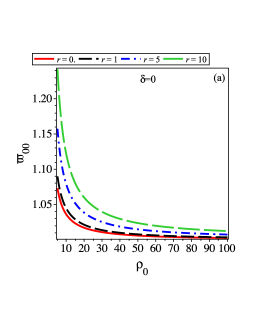
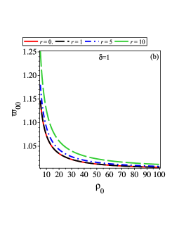
Figure 3: The variations of threshold frequency of absorption $\varpi_{00}$ (in unit of $\epsilon_{g}$) as function of $\rho_{0}$ for several values of the $r$ parameter. In (a) we depicted $\varpi_{00}$ for $\delta=0$ and in (b) $\varpi_{00}$ is plotted for $\delta=1.0$.

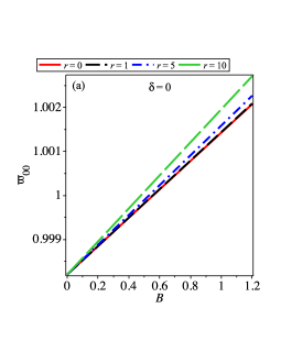
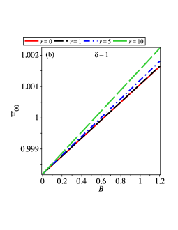
Figure 4: The anti-dot frequency of absorption $\varpi_{00}$ as function of $B$ for several values of the $r$ parameter. In (a) we display $\varpi_{00}$ for absence of a flux field $\delta=0$. In (b) we display $\varpi_{00}$ for $\delta=1.0$

$$\frac{E_{0}^{e}}{\varepsilon_{g}}=\frac{\kappa}{2}\left(\varsigma+1-\delta+\frac{b}{2d}\right)-\frac{2V_{0}}{\varepsilon_{g}},$$ (36)

$$\frac{E_{0}^{h}}{\varepsilon_{g}}=\frac{\kappa^{\prime}}{2}\left(\varsigma+1+\delta-\frac{b}{2d}\right)-\frac{2V_{0}}{\varepsilon_{g}},$$ (37)

where

$$\varsigma=\sqrt{\delta^{2}-\frac{\delta b}{d}+\frac{b^{2}}{2a^{2}\pi^{2}}+\frac{2m_{e}V_{0}\rho_{0}^{2}}{\hbar^{2}}}.$$

Now we study the effect of the AB flux field, the presence and absence of Burgers vector, quantum dot potential and quantum anti-dot potential on the threshold frequency of absorption $\varpi_{00}$ for the typical 2D structure of GaAs, with the following parameters: $V_{0}=0.68346$ meV, $a=5$Å, $d=15$nm, $m_{e}=0.067m_{0}$ and $m_{h}=0.34m_{0}$, where $m_{0}$ is the free electron effective mass. In Fig. 2, we show the variations of the threshold frequency of absorption $\varpi_{00}$ (in units of $\varepsilon_{g}$) for a quantum dot as a function of magnetic field (in units of Tesla) for different values of the ratio $\lambda=b/2d$, which characterize the influence of a screw dislocation and the parameter $r=b/a$.

In Fig. 2(a) shows the variations of the threshold frequency of absorption $\varpi_{00}$ at a fixed energy gap $\varepsilon_{g}$, the chemical potential $V_{0}$ and AB flux $\delta=0$, for four values of positive $\lambda$ and $r$. It is seen that $\varpi_{00}$ increases when the applied magnetic field increases. It is easily seen from the figure that the dependence of $\varpi_{00}$ on $B$ is nonlinear for small applied magnetic fields. On the other hand, by increasing the magnetic field the lines remain linear. It is also noted that when $r$ increases, the curves of frequency $\varpi_{00}$ are pushed up towards of the growth $r$.

The Fig. 2(b) illustrates the behavior of $\varpi_{00}$ for different values of the parameter $r$ and fixed AB flux $\delta=1$. From this figure, we can see that the threshold frequency $\varpi_{00}$ displays a minimum for weak magnetic field. On the other hand, for strong magnetic field behavior is linear. One interesting aspect is that the magnetic flux $\delta$ contributes to the cancellation of screw effect of the model. In the figure this cancellation occurs when $\delta=1$ and $r=1$.

In Fig. 3, we have plots of the variations of the threshold frequency of absorption $\varpi_{00}$ with quantum dot size (in units of $\rho_{0}$). It is seen in Fig. 3(a) that $\varpi_{00}$ decreases when the quantum dot size increases in absence of the AB flux $\delta=0$. In Fig 3(b), we can see that there is an overlap of the curves for $r=0$ and $r=1$ when $\delta=1$, this indicates to us that the AB flux field help to be canceled the screw dislocation.

The effect of the AB flux field on the anti-dot threshold frequency of absorption $\varpi_{00}$ are shown in Fig. 4. In Fig. 4(a), we plot the variation of the anti-dot threshold frequency of absorption $\varpi_{00}$ in the absence of the AB flux field $\delta=0$ as a function of magnetic field. We find that the dependence of $\varpi_{00}$ on $B$ is linear. Fig 4(b) demonstrates the dependence of the anti-dot threshold frequency on $B$ at $\delta=1.0$ with different values of $r$. The behavior of $\varpi_{00}$ is similar frequency of absorption of Fig. 4(a), but the value of $\varpi_{00}$ for $\delta=1$ is always less that frequency of absorption $\varpi_{00}$ when $\delta$ takes the value $0$.

V Concluding Remarks

In conclusion, we have investigated the energy levels for a 2DEG around a screw dislocation under the pseudoharmonic interaction consisting of quantum dot and anti-dot potentials in the presence of an uniform strong magnetic field $B$ and AB flux.

It is known that such a defect on elastic media generates a torsion field that acts on the particle as if an external AB flux were being applied to it. In the usual AB effect, the charged particles in the presence of an uniform magnetic field may be confined to a plane perpendicular to the field lines. This is not possible in the case of torsion, which needs motion in three-dimensional space in order to show up its effects. Because of this fact, we have considered a quasi two-dimensional electron gas confined on a thin interface in such a way that the effects of torsion can manifest. Due to the existence of a screw dislocation, we have considered the effects of two contributions: a covariant term, which comes from the geometric approach in the continuum limit and a noncovariant repulsive scalar potential. Both appear due to elastic deformations on a semiconductor with such kind of topological defect. We have found that this noncovariant term changes significantly the energy levels of electrons in this system. As we have said above, these defects represents a problem since they interfere in the electronic properties of the materials by way of scattering, as we can note by analyzing the non covariant potential in Eq. (3). Therefore, investigations on how this kind of defect influences the dynamics of carriers in common semiconductors are important for the improvement of electronic technology. In our case, the modification introduced by such topological defect in the light absorption coefficient is due to an effective angular momentum induced by torsion. For the threshold frequency value of absorption, we have found that, as the Burgers vector increases, the curves of such frequency are pushed up towards its growth. Moreover, it was noted that the singular effects can take place as well. It is also noted that the AB flux can be tuned in order to cancel the influence of the screw dislocation in these physical quantities.

References

- Landau and Lifschitz (1981) L. D. Landau and E. M. Lifschitz, Quantum Mechanics (Pergamon, Oxford, 1981).
- Aharonov and Bohm (1959) Y. Aharonov and D. Bohm, Phys. Rev. 115, 485 (1959).
- Tan and Inkson (1996) W.-C. Tan and J. C. Inkson, Phys. Rev. B 53, 6947 (1996).
- Ikhdair and Sever (2007) S. Ikhdair and R. Sever, J. Mol. Structure: Theochem 806, 155 (2007).
- Hamzavi et al. (2014) M. Hamzavi, S. M. Ikhdair, and B. J. Falaye, Ann. Phys. 341, 153 (2014).
- Ikhdair et al. (2015) S. M. Ikhdair, B. J. Falaye, and M. Hamzavi, Ann. Phys. 353, 282 (2015).
- Katanaev and Volovich (1992) M. Katanaev and I. Volovich, Ann. Phys. (NY) 216, 1 (1992).
- Kawamura (1978) K. Kawamura, Zeitschrift für Physik B Condensed Matter 29, 101 (1978).
- Bueno et al. (2016) M. Bueno, C. Furtado, and K. Bakke, Physica B: Condensed Matter 496, 45 (2016).
- Bausch et al. (1999a) R. Bausch, R. Schmitz, and L. A. Turski, Phys. Rev. B 59, 13491 (1999a).
- Bausch et al. (1998) R. Bausch, R. Schmitz, and L. A. Turski, Phys. Rev. Lett. 80, 2257 (1998).
- Furtado and Moraes (1999) C. Furtado and F. Moraes, Europhys. Lett. 45, 279 (1999).
- Bakke and Moraes (2012) K. Bakke and F. Moraes, Phys. Lett. A 376, 2838 (2012).
- Lorenci and Jr. (2012) V. A. D. Lorenci and E. S. M. Jr., Phys. Lett. A 376, 2281 (2012).
- Netto et al. (2008) A. S. Netto, C. Chesman, and C. Furtado, Phys. Lett. A 372, 3894 (2008).
- Bausch et al. (1999b) R. Bausch, R. Schmitz, and u. A. Turski, Ann. Phys. (Leipzig) 8, 181 (1999b).
- Taira and Shima (2014) H. Taira and H. Shima, Solid State Communications 177, 61 (2014).
- Slager et al. (2014) R.-J. Slager, A. Mesaros, V. Juričić, and J. Zaanen, Phys. Rev. B 90, 241403 (2014).
- Slager et al. (2016) R.-J. Slager, V. Juričić, V. Lahtinen, and J. Zaanen, Phys. Rev. B 93, 245406 (2016).
- Ikhdair and Hamzavi (2012) S. M. Ikhdair and M. Hamzavi, Physica B: Condensed Matter 407, 4198 (2012).
- Abramowitz and Stegun (1972) M. Abramowitz and I. A. Stegun, eds., Handbook of Mathematical Functions (New York: Dover Publications, 1972).
- Hagen (2008) C. R. Hagen, Phys. Rev. A 77, 036101 (2008).
- Filgueiras et al. (2010) C. Filgueiras, E. O. Silva, W. Oliveira, and F. Moraes, Ann. Phys. (NY) 325, 2529 (2010).
- Atoyan et al. (2004) M. Atoyan, E. Kazaryan, and H. Sarkisyan, Physica E: Low-dimensional Systems and Nanostructures 22, 860 (2004).
- Atoyan et al. (2006) M. Atoyan, E. Kazaryan, and H. Sarkisyan, Physica E: Low-dimensional Systems and Nanostructures 31, 83 (2006).
- Raigoza et al. (2005) N. Raigoza, A. Morales, and C. Duque, Physica B: Condensed Matter 363, 262 (2005).
- Khordad (2010) R. Khordad, Solid State Sciences 12, 1253 (2010).