Vortex lines attached to dark solitons in Bose-Einstein condensates and Boson-Vortex Duality in 3+1 Dimensions

Abstract

We demonstrate the existence of stationary states composed of vortex lines attached to planar dark solitons in scalar Bose-Einstein condensates. Dynamically stable states of this type are found at low values of the chemical potential in channeled condensates, where the long-wavelength instability of dark solitons is prevented. In oblate, harmonic traps, U-shaped vortex lines attached by both ends to a single planar soliton are shown to be long-lived states. Our results are reported for parameters typical of current experiments, and open up a way to explore the interplay of different topological structures. These configurations provide Dirichlet boundary conditions for vortex lines and thereby mimic open strings attached to D-branes in string theory. We show that these similarities can be formally established by mapping the Gross-Pitaevskii theory into a dual effective string theory for open strings via a boson-vortex duality in 3+1 dimensions. Combining a one-form gauge field living on the soliton plane which couples to the endpoints of vortex lines and a two-form gauge field which couples to vortex lines, we obtain a gauge-invariant dual action of open vortex lines with their endpoints attached to dark solitons.

I Introduction

Quantum vortices and planar dark solitons are frequently generated in current experiments with ultracold gases, from Bose-Einstein condensates (BECs) Fetter2009 ; Frantzeskakis2010 to Fermi gases Zwierlein2005 ; Ku2014 ; Ku2016. With phase imprinting techniques, the phase of the superfluid can be arranged to show either continuous $2\pi$ changes around vortex lines, or sudden leaps across the soliton planes. These topological defects, which separate regions with different values of the resulting order parameter, also appear after the quench crossing a second-order phase transition breaking the underlying continuous symmetry known as the Kibble-Zurek mechanism Kibble1976 ; Zurek1985 . The great achievement of techniques in experiments with ultracold gases has directed researchers’ attention towards more complex physical systems presenting nontrivial topologies, which might simulate different types of topological excitations discussed in quantum field theory and string theory. For instance, analogues of cosmic strings in superfluids  Zurek1985 ; Lamporesi2013 and analogues of Dirac monopoles in the spin-1 BEC Savage2003 ; Borgh2012 have been proposed. ³He A-B interfaces and the boundary surface of the two-component BEC have been suggested as analogues of branes in string theory Bradley2007 ; Nitta-1 ; Nitta-2 ; Nitta-3 . Isolated monopoles monopolesinBECs and Dirac monopoles DiracmonopoleBECs have been observed in recent spin-1 BEC experiments.

In this work we show that scalar BECs are also suitable for studying rich structures of topological defects. In spite of the fact that there have been an intensive research about vortices and solitons in scalar BECs, as far as we know, the study of topological structures showing junctions between them has not been performed. Only a particular configuration of this type has been addressed in the context of an effective low-dimensional model in trapped condensates Mateo2013 . Note that in a trapped BEC without dark solitons stable vortex lines which do not form loops have to end at the condensate boundary. Here, within a mean field approach, we address the dynamics of scalar BECs containing vortex lines that extend between soliton stripes. This arrangement makes it possible to find the ends of a vortex line in the bulk of the system, just at the position of the soliton. Configurations of this type will be referred to as open vortex lines, and they provide Dirichlet boundary conditions for the vortex ends. It is interesting to note that they mimic open strings attached to D-branes in string theory, in particular the so-called BIons. Although the arrangements shown in the present work are not generic from the string theory point of view, they might still offer a ground for simulating particular aspects of it. To establish this connection on more formal terms, we show that the Gross-Pitaevskii (GP) theory can be mapped into an effective string theory via the so-called boson-vortex duality.

The rest of the paper is structured as follows. In Section II, we present the mean field model based on the Gross-Pitaevskii energy functional, which is used to describe accurately the dynamics of BECs containing vortices and solitons. In Section III, we propose the boson-vortex duality for open vortex lines ending on dark solitons. The following sections are dedicated to particular realistic configurations fitting into both the GP description and its dual description. First, in Section IV, we consider condensates trapped along their transverse directions and containing axisymmetric vortex lines separated by dark solitons that extend over the cross section of the system. We demonstrate that a 3D condensate endowed with this structure can be a dynamically stable stationary state. Beyond a threshold value for the interaction energy such configuration becomes unstable due to the soliton decay, and the whole system can evolve through new emerging vortex lines. Second, in Section V, we study slightly oblate condensates holding symmetric planar solitons, to which U-shaped vortex lines, that are referred to as half vortex rings, are attached. In this variant configuration, each curved vortex line has both ends on a single dark soliton. We show that, although such stationary state is dynamically unstable, it has a long lifetime. The ultimate decay of the soliton shows chaotic behaviors of vortex lines, which might be related to quantum turbulence processes. A common feature of both configurations is the presence of vortex line pairs separated by the soliton plane. We finish with the conclusions in Section VI, where we emphasize that the topological states considered in this paper are feasible to be realized under current experimental techniques.

II Gross-Pitaevskii Model

We follow a mean-field approach for modeling dilute gases of repulsive interacting bosons making Bose-Einstein condensates at zero temperature. The state of such a system is described by a complex order parameter $\Psi(\mathbf{r},t)$, whose dynamics is determined by the non-relativistic GP Lagrangian density:

$${\cal L}_{GP}=\frac{i\hbar}{2}\left(\Psi\frac{\partial\Psi^{*}}{\partial t}-\Psi^{*}\frac{\partial\Psi}{\partial t}\right)-H_{\rm GP},$$ (1)

where the energy density is given by

$$H_{\rm GP}=\frac{\hbar^{2}}{2m}|\nabla\Psi|^{2}+\frac{g}{2}\left(|\Psi|^{2}-|\Psi_{0}|^{2}\right)^{2}.$$ (2)

Here $g=4\pi\hbar^{2}a/m$ is the interaction parameter, characterized by the $s$-wave scattering length $a$ and the atomic mass $m$. Note that the energy is measured relative to the ground state $\Psi_{0}(\mathbf{r},t)=\psi_{0}(\mathbf{r})\,\exp(-i\mu\,t/\hbar)$ with chemical potential $\mu$. For homogeneous systems, $\Psi_{0}$ is a real constant, apart from a global phase, and $\mu$ fixes the value of the uniform density $|\Psi_{0}|^{2}=\mu/g$. In the presence of an external potential $V(\mathbf{r})$, a local chemical potential $\mu_{l}(\mathbf{r})=\mu-V(\mathbf{r})$ can be defined, which in the limit of high interaction energy, or Thomas-Fermi regime, allows to approximate the non-uniform ground-state density by $|\Psi_{0}(\mathbf{r})|^{2}=\mu_{l}(\mathbf{r})/g$. In this way, we will use Eq. (1) as a unified model for both homogeneous and non-homogeneous systems. In the latter case, this means that when the system is closed, the energy is measured with respect to the ground state having the same chemical potential, and thus, in general, a different number of particles. For non-homogeneous systems, we will consider harmonic trapping potentials with cylindrical symmetry $V(\mathbf{r})=V_{z}(z)+V_{\perp}(r_{\perp})=m\omega_{z}^{2}z^{2}/2+m\omega_{\bot}^{2}r_{\perp}^{2}/2$, having an aspect ratio $\lambda=\omega_{z}/\omega_{\perp}$, where the transverse coordinates are $(\theta,r_{\perp})=(\tan^{-1}(y/x),\sqrt{x^{2}+y^{2}})$. As a length unit, we define the characteristic length of the transverse trap $a_{\perp}=\sqrt{\hbar/m\omega_{\perp}}$.

The equation of motion corresponding to the Lagrangian density ${\cal L}_{GP}$ is the time-dependent GP equation

$$i\hbar\frac{\partial\Psi}{\partial t}=\left(-\frac{\hbar^{2}}{2m}\nabla^{2}+g(|\Psi|^{2}-|\Psi_{0}|^{2})\right)\Psi.$$ (3)

Its stationary solutions with chemical potential $\mu$, that is $\Psi(\mathbf{r},t)=\psi(z,\theta,r_{\perp})$, fulfill the time-independent GP equation

$$\left(-\frac{\hbar^{2}}{2m}\nabla^{2}+g(|\psi|^{2}-|\psi_{0}|^{2})\right)\psi=0.$$ (4)

III Duality

III.1 Effective string action

The boson-vortex duality is a powerful tool to study the dynamics of vortex rings Lund1976 ; ZeePaper ; Gubser ; Gubser16 ; Horn2015 . It has been demonstrated that the dual description of the GP theory in 3+1 dimensions is equivalent to a certain type of effective string theory ZeePaper ; Franz ; Gubser . In this paper we extend the dual mapping to open vortex lines and argue that dark solitons in the original GP theory could play the role of D-branes in the effective string theory by introducing a pinned boundary condition for vortex lines BECstring1 . In the following, for simplicity we set the trapping potential to be zero, i.e. $V(\mathbf{r})=0$.

Introducing the Madelung transformation $\Psi=\sqrt{\rho}\,e^{i\phi}$, the equivalent expression of the GP Lagrangian density Eq. (1) in terms of the condensate density $\rho$ and the phase $\phi$ reads

$$\mathcal{L}_{GP}\simeq-\hbar\rho\dot{\phi}-\rho\frac{\hbar^{2}}{2m}(\nabla\phi)^{2}-\frac{g}{2}(\rho-\rho_{0})^{2}\,,$$ (5)

where we neglect the quantum pressure term $\sim(\nabla\sqrt{\rho})^{2}$, which should be valid at long wavelengths (the hydrodynamic limit) that we are interested in. We rewrite the quadratic term $-\rho{\hbar^{2}}(\nabla\phi)^{2}/{2m}$ via the so-called Hubbard-Stratanovich transformation HS , and obtain the dual representation of the original theory Eq. (5) :

$$\mathcal{L}^{*}_{GP} \simeq -\hbar\rho\dot{\phi}-\hbar\nabla\phi\cdot\mathbf{f}+\frac{m}{2\rho}\mathbf{f}\cdot\mathbf{f}-\frac{g}{2}(\rho-\rho_{0})^{2}$$ (6)

$$= -\hbar f^{\mu}\partial_{\mu}\phi+\frac{m}{2\rho}\mathbf{f}\cdot\mathbf{f}-\frac{g}{2}(\rho-\rho_{0})^{2},$$

where $\partial_{\mu}\equiv(\partial_{t},\nabla)$, and $\mathbf{f}$ is an auxiliary three-vector, which is also the space-like components of the four-vector $f^{\mu}\equiv(\rho,\mathbf{f})$. The physical meaning of the field $\mathbf{f}$ becomes clear by evaluating its equation of motion $\mathbf{f}=\rho\frac{\hbar}{m}\nabla\phi$, which matches the superfluid current $\mathbf{J}$ in the GP theory described by Eq. (1) Lund1976 .

Let us now decompose the phase $\phi$ into a non-singular part and a few singular parts related to the topological defects:

$$\phi=\phi_{g}+\phi_{\rm cv}+\phi_{\rm ov}+\phi_{\rm s},$$ (7)

where $\phi_{g}$ is the smooth phase, which is the Goldstone mode associated with the $U(1)$ symmetry breaking, $\phi_{\rm cv}$ is the phase of vortex rings, $\phi_{\rm ov}$ is the phase of open vortex lines, and $\phi_{\rm s}$ represents the phase of dark solitons. Note that Eq. (7) just means that $\phi_{\rm cv}$, $\phi_{\rm ov}$ and $\phi_{\rm s}$ have singularities, and they may still contain smooth parts. The action of the non-singular part $\phi_{g}$ reads

$$\mathcal{S}_{g} = \int d^{4}x\left(-\hbar f^{\mu}\partial_{\mu}\phi_{g}\right)$$

$$= \hbar\int d^{4}x\left[\partial_{\mu}f^{\mu}\phi_{g}-\partial_{\mu}(f^{\mu}\phi_{g})\right].$$

By integrating out the smooth phase $\phi_{g}$ in the bulk, we obtain

$$\partial_{t}\rho+\nabla\cdot\mathbf{f}=\partial_{\mu}f^{\mu}=0,$$ (9)

which can be solved by

$$f^{\mu}=\frac{1}{2}\epsilon^{\mu\nu\lambda\sigma}\partial_{\nu}B_{\lambda\sigma}\,,$$ (10)

where $\epsilon^{\mu\nu\lambda\sigma}$ is the totally-antisymmetric tensor, and $B_{\lambda\sigma}$ is an antisymmetric rank-2 gauge field. Note that $f^{\mu}$ is invariant under the gauge transformation $B_{\mu\nu}\rightarrow B_{\mu\nu}+\partial_{\mu}\Lambda_{\nu}-\partial_{\nu}\Lambda_{\mu}$, where $\Lambda_{\nu}$ is an arbitrary four vector.

In the dual description, the action of a vortex ring in 3+1 dimensions has already been proposed Lund1976 ; ZeePaper ; Franz ; Gubser . In this paper we focus on open vortex lines. For an open vortex line the action reads

$$\mathcal{S}_{\rm ov} = \int d^{4}x\left(-\hbar f^{\mu}\partial_{\mu}\phi_{\rm ov}\right)$$

$$= -\frac{\hbar}{2}\int d^{4}x\epsilon^{\mu\nu\lambda\sigma}\partial_{\nu}B_{\lambda\sigma}\partial_{\mu}\phi_{\rm ov}$$

$$= \frac{\hbar}{2}\int d^{4}x\left[\partial_{\mu}(\epsilon^{\mu\nu\lambda\sigma}B_{\lambda\sigma}\partial_{\nu}\phi_{\rm ov})-B_{\mu\nu}\epsilon^{\mu\nu\lambda\sigma}\partial_{\lambda}\partial_{\sigma}\phi_{\rm ov}\right].$$

We elaborate on these terms by considering a vortex line which is parallel to the z-axis, whose topological nature can be seen from the term

$$\int d^{2}x\,\epsilon^{zt\lambda\sigma}\partial_{\lambda}\partial_{\sigma}\phi_{\rm ov}=2\pi.$$ (12)

The topological defects produced by vortex lines can be introduced explicitly through

$$\epsilon^{\mu\nu\lambda\sigma} \partial_{\lambda}\partial_{\sigma}\phi_{\rm ov}$$

$$=-2\pi\sum_{i}\int_{\Sigma_{i}}d\tau d\sigma\epsilon^{\alpha\beta}\partial_{\alpha}X^{\mu}\partial_{\beta}X^{\nu}\delta^{4}(x^{\mu}-X^{\mu}),$$

where $\Sigma_{i}$ is the worldsheet spanned by the $i$-th vortex line, and $\alpha,\,\beta\in\{0,1\}$ label the worldsheet coordinates. $\epsilon^{\alpha\beta}$ is a rank-2 antisymmetric tensor, and we set $\epsilon^{10}=1$. The space $\sigma\in[\sigma_{0},\sigma_{1}]$, and the time $\tau$ is chosen to be $t$. $X^{\mu}=X^{\mu}(\tau,\sigma)$ stands for the coordinates of a vortex line, namely $X^{0}=t$, $\mathbf{X}=(x,y,z)$. Hence, the bulk action of the open vortex line reads

$$S^{\rm v}_{\rm bulk} = -\frac{\hbar}{2}\int d^{4}xB_{\mu\nu}\epsilon^{\mu\nu\lambda\sigma}\partial_{\lambda}\partial_{\sigma}\phi_{\rm ov}$$

$$= \frac{\eta}{2}\sum_{i}\int_{\Sigma_{i}}d\tau d\sigma B_{\mu\nu}\epsilon^{\alpha\beta}\partial_{\alpha}X^{\mu}\partial_{\beta}X^{\nu},$$

where $\eta\equiv 2\pi\hbar$ and $B_{\mu\nu}=B_{\mu\nu}(X^{\mu})$.

Suppose that an ($x$-$y$)-planar dark soliton, to which a vortex line can be attached, is located at $z=z_{0}$. We make use of the soliton property of producing a localized $\pi$ phase jump by crossing the soliton plane, i.e.

$$\partial_{z}\phi_{s}(t,x,y,z)=\pi\int d^{3}\sigma\,\delta^{3}(x^{a}-Y^{a}(\sigma_{i}))\delta(z-z_{0}),$$

$$\partial_{a}\phi_{s}(t,x,y,z)=\ell\int d^{3}\sigma\,\partial_{a}\hat{\phi}_{s}(\sigma_{i})\,\delta^{3}(x^{a}-Y^{a}(\sigma_{i}))\delta(z-z_{0}),$$ (15)

where $\sigma_{i}$ ($i$ = 1, 2, 3) are the coordinates on the dark soliton plane, $Y^{a}(\sigma_{i})\in\{t,x,y\}$ is the map from $\sigma_{i}$ to the spacetime coordinates, $\ell$ is a length scale inserted for dimensional reasons, and $\hat{\phi}_{s}(\sigma_{i})$ is the transverse phase defined only along the dark soliton plane, which in turn contains a smooth part and a singular part. In addition, the superfluid current along the $z$-direction vanishes at the soliton plane

$${\rm J}^{z}(t,x,y,z_{0})=0,$$ (16)

which implies $f^{z}(t,x,y,z_{0})=0$ and thus imposes a constraint on the $B$-field, according to Eq. (10). Consequently, the boundary term in the action Eq. (III.1) vanishes on the dark soliton surface $-\hbar\int d^{3}xf^{z}(z_{0},x,y,t)\phi_{g}=0$. As a result, the action for the dark soliton is

$$\mathcal{S}_{s}=\int d^{4}x\left(-\hbar f^{\mu}\partial_{\mu}\phi_{s}\right)=-\hbar\int d^{3}x\left(\ell f^{a}\partial_{a}\hat{\phi}_{s}\right).$$ (17)

Combining the boundary term in the action of the open vortex Eq. (III.1):

$$\frac{\hbar}{2}\int d^{3}x\,\epsilon^{zabc}B_{bc}\partial_{a}\phi_{\rm ov}\,,$$ (18)

with a,b,c $\in\{t,x,y\}$, and the dark soliton action Eq. (17), we obtain the boundary action

$$\mathcal{S}^{\rm v}_{\rm boundary}=-\hbar\int d^{3}x\left(\ell f^{a}-\frac{1}{2}\epsilon^{abc}B_{bc}\right)\partial_{a}\hat{\phi}_{s}.$$

Here we made the identification $\phi_{\rm ov}(z\rightarrow z^{\pm}_{0},x,y,t)=\hat{\phi}_{s}(x,y,t)$, which implies that the endpoints of the open vortex lines are the vortex excitations living on the soliton surface ($z\rightarrow z^{\pm}_{0}$). As it has previously been done for $\phi_{g}$, integrating out the smooth part of $\hat{\phi}_{s}$ leads to

$$\partial_{a}(\ell f^{a}-\frac{1}{2}\epsilon^{abc}B_{bc})=0\,,$$ (20)

whose solution is

$$\ell f^{a}-\frac{1}{2}\epsilon^{abc}B_{bc}=\frac{1}{2}\epsilon^{abc}F_{bc},$$ (21)

where $F_{ab}\equiv\partial_{a}A_{b}-\partial_{b}A_{a}$ is the field strength of $A_{a}$, and $A_{a}$ is a one-form gauge field living on the dark soliton surface ($z\rightarrow z^{\pm}_{0}$). Therefore, we are left with the singular part $\hat{\phi}^{s}_{s}$ of $\hat{\phi}_{s}$

$$\mathcal{S}^{\rm v}_{\rm boundary} = -\hbar\int d^{3}x\frac{1}{2}\epsilon^{abc}F_{bc}\partial_{a}\hat{\phi}^{s}_{s}$$ (22)

$$= -\frac{1}{2}\hbar\int d^{3}x\epsilon^{abc}(\partial_{b}A_{c}-\partial_{c}A_{b})\partial_{a}\hat{\phi}^{s}_{s}$$

$$= -\hbar\int d^{3}xA_{a}(\epsilon^{abc}\partial_{b}\partial_{c}\hat{\phi}^{s}_{s}),$$

and for the endpoints of vortex lines, similar to Eqs. (12)–(III.1), we get

$$\epsilon^{abc}\partial_{b}\partial_{c}\hat{\phi}^{s}_{s}=-2\pi\sum_{i}\int_{\partial\Sigma_{i}}d\tau\partial_{\tau}X^{a}\delta^{3}(x^{a}-X^{a}(\tau)),$$ (23)

where $\partial\Sigma_{i}$ is the boundary of the worldsheet $\Sigma_{i}$, and $X^{a}(\tau)$ are the coordinates of an endpoint of a vortex line, namely $X^{0}=t$, $\mathbf{X}=(x,y)$. Then we obtain

$$\mathcal{S}^{\rm v}_{\rm boundary} = -\hbar\int d^{3}xA_{a}(\epsilon^{abc}\partial_{b}\partial_{c}\hat{\phi}^{s}_{s})$$ (24)

$$= \eta\sum_{i}\int_{\partial\Sigma_{i}}d\tau A_{a}\partial_{\tau}X^{a},$$

where $A^{a}=A^{a}(X^{a})$.

In terms of the field strengths, the last two terms of the action Eq. (6) can be written as

$$S_{\rm gauge} =\frac{m}{2\rho}\mathbf{f}\cdot\mathbf{f}-\frac{g}{2}(\rho-\rho_{0})^{2}$$

$$=-\frac{g}{4\ell}\int d^{3}x\,(\widetilde{F}+\widetilde{B})^{2}-\,\frac{g}{2}\int d^{4}x\,\,h_{3}^{2}.$$ (25)

Near $\rho\simeq\rho_{0}$, $H_{\mu\nu\lambda}\equiv\partial_{\mu}B_{\nu\lambda}+\partial_{\nu}B_{\lambda\mu}+\partial_{\lambda}B_{\mu\nu}\simeq H^{0}_{\mu\nu\lambda}+h_{\mu\nu\lambda}$, where $H^{0}_{\mu\nu\lambda}$ is the background field with $H^{0}_{123}=\rho_{0}$, and the fluctuations are given by $h_{3}^{2}=h_{\mu\nu\lambda}h^{\mu\nu\lambda}/6$, through the metric $\eta_{\mu\nu}=\textrm{diag}\{-c_{s}^{2},\,1,\,1,\,1\}$ determined by the speed of sound $c_{s}=\sqrt{g\rho_{0}/m}$. $\widetilde{F}$ and $\widetilde{B}$ are the fluctuations of $F$ and $B$ on the soliton plane respectively.

Collecting all the contributions, we finally obtain the following dual description of open vortex lines:

$$\mathcal{S}^{\ast} = S^{\rm v}_{\rm bulk}+S^{\rm v}_{\rm boundary}+S_{\rm gauge}$$ (26)

$$= \frac{\eta}{2}\sum_{i}\int_{\Sigma_{i}}d\sigma d\tau\,B_{\mu\nu}\epsilon^{\alpha\beta}\partial_{\alpha}X^{\mu}\,\partial_{\beta}X^{\nu}$$

$$+\,\eta\sum_{j}\int_{\partial\Sigma_{j}}d\tau\,A_{a}\,\partial_{\tau}X^{a}-\frac{g}{4\ell}\int d^{3}x\,(\widetilde{F}+\widetilde{B})^{2}$$

$$-\,\frac{g}{2}\int d^{4}x\,\,h_{3}^{2}\,.$$

The summation over $\Sigma_{i}$ includes all the vortex lines and the summation over $\partial\Sigma_{j}$ includes all the endpoints of vortex lines attached to dark solitons. It is important to note that the resulting action Eq. (26) is invariant under the gauge transformations Zwiebach :

$$B_{\mu\nu} \rightarrow B_{\mu\nu}+\partial_{\mu}\Lambda_{\nu}-\partial_{\nu}\Lambda_{\mu},$$ (27)

$$A_{a} \rightarrow A_{a}-\Lambda_{a}.$$ (28)

The action given in Eq. (26) has two aspects. First of all, it provides a hydrodynamic description of open vortex lines in scalar BECs, which is useful to study the dynamics of open vortex lines with Dirichlet boundary conditions and vortex-sound interactions. On the other hand, it can be viewed as an effective open string action without the tension term, or equivalently an action in the large $B$-field limit, in the presence of D-branes. Hence, the dual theory Eq. (26) might provide a possibility to test some aspects of string theory in BEC experiments.

III.2 Equation of motion

In the following we will discuss a simple example of the action Eq. (26). From now on we will only consider a single vortex line whose endpoints are attached to two parallel dark solitons. Here, for simplicity, we ignore the dynamics of the dark solitons and treat them as hard walls. We will also assume that the fluctuations of $B_{\mu\nu}$ and $A_{a}$ in space-time are small, and hence the field strength parts in $S_{\rm gauge}$ can be neglected since they provide higher order terms.

In order to have non-trivial dynamics of a single vortex line, we need to introduce in the action Eq. (26) a phenomenological tension term, which plays the role of kinetic energy of vortices. This term has been neglected up to now because of the assumption of infinitely thin topological defects. Such assumption implies the lack of vortex cores and also the absence of a “physical” mass of the vortex lines, which is responsible, among other dynamical effects, for the buoyancy-like forces in inhomogeneous backgrounds Konotop2004 . As a consequence, the tension term can be seen as a remnant of the core structure of the vortices in the hydrodynamic limit.

We introduce the tension term in Eq. (26) by adding a Polyakov string action Zwiebach proportional to the the string tension $T$:

$$\mathcal{S}^{\rm single} = \frac{T}{2c_{s}}\int_{\Sigma}d\sigma d\tau\sqrt{-h}\,h^{\alpha\beta}\,\eta_{\mu\nu}\,\partial_{\alpha}X^{\mu}\partial_{\beta}X^{\nu}$$ (29)

$$+\frac{\eta}{2}\int_{\Sigma}d\sigma d\tau\,B_{\mu\nu}\epsilon^{\alpha\beta}\partial_{\alpha}X^{\mu}\partial_{\beta}X^{\nu}$$

$$+\,\eta\int_{\partial\Sigma}d\tau\,A_{a}\,\partial_{\tau}X^{a},$$

where $h^{\alpha\beta}=\rm diag\{-1/c^{2}_{s},1\}$ is the worldsheet metric, and $\sqrt{-h}=\sqrt{-{\rm det}(h_{\alpha\beta})}=c_{s}$. $T$ has the standard dimension $[E]/[L]$ for the string tension and in terms of BEC units $T\sim\pi\hbar^{2}\rho_{0}/2m$.

Considering a small variation $\delta X^{\mu}$ on top of the background vortex configuration $X^{\mu}$ bgdfield , the variation of the action to the leading order in $\delta X^{\mu}$ reads

$$\delta S^{\rm single} =\frac{T}{2}\int_{\Sigma}d\sigma\,d\tau\,2\partial_{\alpha}(\delta X^{\mu})\partial^{\alpha}X_{\mu}$$

$$\quad+\frac{\eta}{2}\int_{\Sigma}d\sigma\,d\tau\,B_{\mu\nu}\epsilon^{\alpha\beta}(\partial_{\alpha}\delta X^{\mu})\partial_{\beta}X^{\nu}$$

$$\quad+\frac{\eta}{2}\int_{\Sigma}d\sigma\,d\tau\,B_{\mu\nu}\epsilon^{\alpha\beta}(\partial_{\alpha}X^{\mu})(\partial_{\beta}\delta X^{\nu})$$

$$\quad+\frac{\eta}{2}\int_{\Sigma}d\sigma\,d\tau\,(\partial_{\rho}B_{\mu\nu})(\delta X^{\rho})\epsilon^{\alpha\beta}\partial_{\alpha}X^{\mu}\partial_{\beta}X^{\nu}$$

$$\quad+\eta\int_{\partial\Sigma}d\tau\,(\partial_{b}A_{a})(\delta X^{b})\partial_{\tau}X^{a}$$

$$\quad+\eta\int_{\partial\Sigma}d\tau\,A_{a}\partial_{\tau}(\delta X^{a})$$

$$= \quad-T\int_{\Sigma}d\sigma d\tau\,(\delta X^{\mu})\partial^{\alpha}\partial_{\alpha}X_{\mu}$$

$$\quad+\frac{\eta}{2}\int_{\Sigma}d\sigma d\tau\,H_{\mu\lambda\nu}(\delta X^{\mu})\epsilon^{\alpha\beta}\partial_{\alpha}X^{\lambda}\partial_{\beta}X^{\nu}$$

$$\quad+T\int_{\partial\Sigma}d\tau\,(\delta X^{a})\partial_{\sigma}X_{a}\,$$

$$\quad+\eta\int_{\partial\Sigma}d\tau\,(B_{ab}+F_{ab})(\delta X^{a})\partial_{\tau}X^{b}.$$ (30)

Hence the equation of motion of the vortex line in the bulk is given by

$$-T\partial_{\alpha}\partial^{\alpha}X_{\mu}+\frac{\eta}{2}\epsilon^{\alpha\beta}H_{\mu\lambda\nu}\partial_{\alpha}X^{\lambda}\partial_{\beta}X^{\nu}=0,$$

and the dynamics of the endpoints reads

$$T\,\partial_{\sigma}X_{a}\big{|}_{\sigma_{1}}+\eta\,(B_{ab}+F_{ab})\partial_{\tau}X^{b}\big{|}_{\sigma_{1}}=0$$ (32)

and

$$-T\,\partial_{\sigma}X_{a}\big{|}_{\sigma_{0}}-\eta\,(B_{ab}+F_{ab})\partial_{\tau}X^{b}\big{|}_{\sigma_{0}}=0\,.$$ (33)

We now consider a special situation. In the bulk $H_{0ij}=0$, and $H_{ijk}=\rho_{0}\epsilon_{ijk}$. On the boundaries $A_{0}=0$, $\partial_{\tau}A_{a}(\sigma_{1})=\partial_{\tau}A_{a}(\sigma_{0})=0$ and $B_{nm}(\sigma_{1})=B_{nm}(\sigma_{0})=\rho_{0}\epsilon_{nm}$. Here $m,n=1,2$. For this special case we obtain the following equations

$$0 = T\left(\frac{\partial^{2}X_{i}}{\partial\sigma^{2}}-\frac{1}{c^{2}_{s}}\frac{\partial^{2}X_{i}}{\partial\tau^{2}}\right)-\frac{\eta}{2}\epsilon^{\alpha\beta}\rho_{0}\epsilon_{ijk}\partial_{\alpha}X^{j}\partial_{\beta}X^{k}\,,$$

$$0 = T\,\partial_{\sigma}X_{n}+\eta\,\rho_{0}\epsilon_{nm}\partial_{\tau}X^{m}\,.$$ (34)

Here we only look for a static solution. For a static vortex line,

$$\frac{\partial^{2}X_{i}}{\partial\sigma^{2}}=0,\quad\partial_{\sigma}X_{n}=0.$$ (35)

The general solution would be

$$x=a_{1}\sigma+a_{2},\quad y=b_{1}\sigma+b_{2},\quad z=c_{1}\sigma+c_{2},$$ (36)

where $a_{1}$, $a_{2}$, $b_{1}$, $b_{2}$, $c_{1}$ and $c_{2}$ are constants. By choosing the proper coordinates and taking into account the boundary conditions, the static solution reads

$$x=a_{2},\quad y=b_{2},\quad z(\sigma)=c_{1}\sigma+c_{2},$$ (37)

which describes a static open vortex line between two dark solitons. Note that this vortex line satisfies Neumann boundary conditions along $x$ and $y$ directions, while fulfills Dirichlet boundary condition along $z$ direction. If we replace the current boundary conditions with periodic boundary conditions, Eq. (35) would give a trivial solution, which means that vortex rings must propagate as it is well-known.

In the next two sections we show that such static vortex-soliton composite topological excitations can indeed be found in the GP theory. For the sake of comparison with realistic parameters used in current experiments of ultracold gases, in what follows we report numerical results for systems composed of ⁸⁷Rb atoms, with scattering length $a=5.29$ nm, confined by harmonic potentials with angular frequencies in the range $2\pi\times[10-100]$ Hz.

IV Open vortex lines

IV.1 Configurations

In this section, we consider elongated condensates along the axial $z$-direction (assuming $\omega_{z}=0$) and isotropic trapping in the transverse plane, providing the system with a channeled structure. In particular, we will consider stationary states containing vortex lines attached to solitons. The simplest configuration of this type, containing a single dark soliton, is shown in Fig. LABEL:Fig1_os. In order to realize this simple configuration we have devised a channeled, cylindrical geometry with an axisimetric vortex line:

$$\psi(z,\theta,r_{\perp})=\psi_{1}(z,r_{\perp})e^{i\theta}\,,$$ (38)

where $\psi_{1}(z,r_{\perp})$ is a real function. After substituting in Eq. (4), the vortex solution gives

$$-\frac{\hbar^{2}}{2m}\left(\partial_{z}^{2}+\nabla_{\perp}^{2}-\frac{1}{r_{\perp}^{2}}\right)\psi_{1}+V_{\perp}\psi_{1}+g\left|\psi_{1}\right|^{2}\psi_{1}=\mu\psi_{1},$$ (39)

where $\nabla_{\perp}^{2}=\partial_{r_{\perp}}^{2}+\partial_{r_{\perp}}/r_{\perp}$ and $V_{\perp}$ accounts for the transverse confinement. This is the stationary equation for a vortex state that generates a tangential velocity field $\mathbf{v}=\hbar\nabla\arg(\psi)/m$ around the $z$-axis: $\mathbf{v}(r_{\perp})={\hbar\mathbf{u_{\theta}}}/{mr_{\perp}}$, where $\mathbf{u_{\theta}}$ is the unit tangent vector.

Next, we search for solutions to the nonlinear Eq. (39) including a dark soliton along the axial direction. An analytical ansatz for this configuration is

$$\psi_{1}(z,r_{\perp})=r_{\perp}\chi(r_{\perp})\,\tanh\left(\frac{z}{\xi(r_{\perp})}\right)\,,$$ (40)

where $\xi(r_{\perp})=\hbar/\sqrt{mg|\chi(r_{\perp})|^{2}}$ defines a radius-varying healing length through the Thomas-Fermi density profile $|\chi(r_{\perp})|^{2}=\mu_{l}(r_{\perp})/g$ of a system without the vortex. This expression follows the ansatz introduced in Ref. Mateo2014 for 3D dark solitons in channeled condensates, and gives a good estimate in the strongly interacting regime, where the Thomas-Fermi approximation applies. Although the $r_{\perp}$ factor of Eq. (40) accounts for the vortex core in a quite simple manner, which is characteristic of the corresponding noninteracting system, it will turn out to be efficient in getting numerical convergence to the real stationary state.

By using the ansatz Eq. (40) for open vortex lines, we have followed a Newton method to find the exact numerical solution to the full GP Eq. (4). Fig. LABEL:Fig1_os shows the features of this configuration (without axial confinement) around a vortex-soliton junction, which leads to Dirichlet boundary conditions for the vortex end points. The panel Fig. LABEL:Fig1_os(a), presenting a semi-transparent density isocontour of the condensate at 5 $\%$ of maximum density, shows how the presence of the dark soliton breaks the system into two phase-separated subsets containing corresponding axisymmetric vortices. These vortices are different entities, as can be seen in the detailed view of panel Fig. LABEL:Fig1_os(b). The dark soliton twists their relative phase in $\pi$ radians along the $z$-axis for every value of the azimuthal coordinate $\theta$, and their end points lay aligned on opposite sides of the soliton membrane. Characteristic features of the system are depicted in Fig. LABEL:Fig1_os(b)-(c): the axial phase jump for a given azimuthal angle, and the axial density of the condensate after integration over the transverse coordinates $n_{1}(z)=\int|\psi(z,r_{\perp},\theta)|^{2}r_{\perp}dr_{\perp}d\theta$ times the scattering length. The stability of this and more complex configurations within the GP theory will be analyzed in Sections IV-V in realistic condensates.

It is important to note that for scalar BECs, a hypothetical configuration with a single vortex line attached to a dark soliton is not stationary. For such a case, the phase difference between the left and the right side of the dark soliton changes continuously along the azimuthal angle from $0$ to $\pi$. As a consequence, the superfluid density can not be zero all along the soliton plane, and the superfluid velocity is non-uniform, which makes this a transient configuration.

It is also interesting to consider configurations containing two nearby dark solitons, as the one presented in Fig. 2 for a condensate having $\mu=4\,\hbar\omega_{\perp}$. In this arrangement, the interaction between solitons is mediated in the long range by the vortex lines. Fig. 2(a) shows the isocontour at 5 $\%$ of maximum density colored according to the complex phase pattern produced by the interplay of solitons and vortices. As can be deduced from Fig. 2(b)-(c), presenting the axial phase and density of the system, the inner region between solitons is characterized by a state that differs in the phase from that of the outer region.

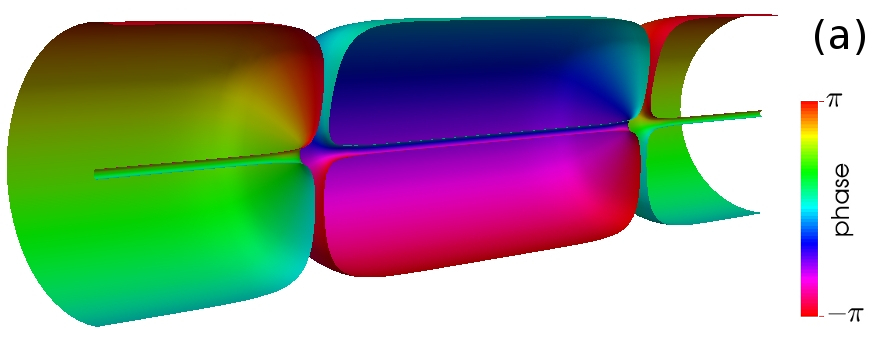
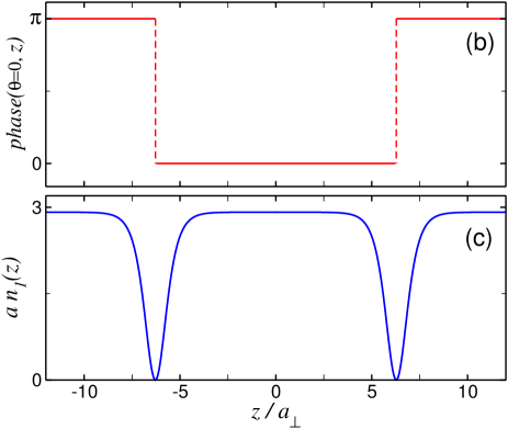
Figure 2: Two dark solitons connected by axisymmetric vortices in a channeled condensate with $\mu=4\,\hbar\omega_{\perp}$. (a) Perspective view of the density isocontour at 5 $\%$ of maximum density, colored by phase, after removing half condensate for better visualization. (b)-(c) Same as in Fig. LABEL:Fig1_os.

IV.2 Stability

States containing open vortex lines, as exemplified by Figs. LABEL:Fig1_os and  2, are dynamically stable as long as the dark soliton does not decay. As it is known, the decay of multidimensional dark solitons is produced by long-wavelength modes excited on the soliton membrane, through the so-called snaking instability Kuznetsov1988 . However, such modes can be prevented to appear by means of a tight transverse trap, which confines the system to a reduced cross section. In terms of the chemical potential, and in the absence of a vortex, a channeled dark soliton is stable up to the value $\mu=2.65\,\hbar\omega_{\perp}$ Mateo2014 . One could expect that, since the zero point energy introduced by an axisymmetric vortex in the harmonic trap increases in one energy quantum $\hbar\omega_{\perp}$ relative to the ground state, the stability threshold for dark solitons in the presence of the vortex would increase by the same amount relative to the case without vortex. This argument leads to a threshold localized at $\mu=3.65\,\hbar\omega_{\perp}$. As we will see below, it is a reasonable estimate, since the unstable frequencies that can be found under such value are very small. We have observed that these latter instabilities are derived from the junction vortex–soliton (i.e. the boundary conditions imposed by the soliton on the vortex ends), and possess slightly different amplitudes for different axial lengths of the computational domain considered. For particular axial lengths, it is possible to find dynamically stable configurations with chemical potentials below the mentioned threshold [as the case shown in Fig. 4(a)], and in the general case our results show that the system presents long lifetimes in the characteristic units of the trap.

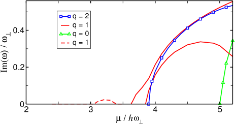
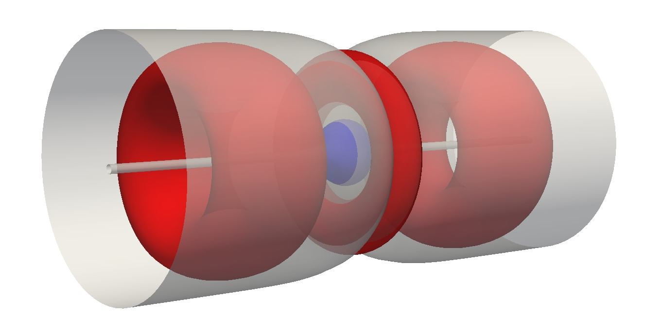
Figure 3: Frequencies of unstable modes for open vortex lines as a function of the chemical potential (upper panel). The curves correspond to the three lowest azimuthal quantum numbers $q$ of the excitation modes (see text). The $q=1$ dashed line accounts for excitations derived from the vortex-soliton junction, an example of which is given in the lower panel for a condensate with $\mu=\,3.2\hbar\omega_{\perp}$. The density isocontours (lower panel) correspond to the condensate (semi-transparent contour), and to two different unstable modes (colour contours) having zero (inner blue contour) and $2\hbar$ (outer red toroidal contours) angular momentum per particle.

A quantitative analysis of the dynamical stability can be done through the Bogoliubov equations (BE) for the linear excitations of the condensate. To this aim, we introduce the linear modes $\{u(\mathbf{r}),v(\mathbf{r})\}$ with energy $\mu\pm\hbar\omega$ to perturb the equilibrium state, i.e. $\Psi(\mathbf{r},t)=\psi+\sum_{\omega}(u\,e^{-i\omega t}+v^{*}e^{i\omega t})$. After substitution in Eq. (3), and keeping terms up to first order in the perturbation, we get

$$\left(H_{L}+2g|\psi|^{2}\right)u+g\psi^{2}v=\hbar\omega\,u\,,$$ (41a)

$$-g(\psi^{*})^{2}u-\left(H_{L}+2g|\psi|^{2}\right)v=\hbar\omega\,v\,,$$ (41b)

where $H_{L}$ is the linear part of the Hamiltonian in Eq. (3), i.e. $H_{L}=-\hbar^{2}\nabla^{2}/2m+V(\mathbf{r})-\mu$. These equations allow to identify the dynamical instabilities of the stationary state $\psi$, which are associated to the existence of $\omega$ frequencies with non-vanishing imaginary parts.

For the vortex state $\psi(z,\theta,r_{\perp})=\psi_{1}(z,r_{\perp})e^{i\theta}$ the BE Eq. (41) read

$$\left(H_{L}+2g\psi_{1}^{2}\right)u+g\psi_{1}^{2}e^{i2\theta}v=\hbar\omega\,u\;,$$ (42a)

$$-g{\psi_{1}}^{2}e^{-i2\theta}u-\left(H_{L}+2g\psi_{1}^{2}\right)v=\hbar\omega\,v\;.$$ (42b)

We search for the modes of the functional form $\{u(z,r_{\perp})e^{i(q+1)\theta},v(z,r_{\perp})e^{i(q-1)\theta}\}$ with $q=0,\pm 1,\pm 2,...$. After adding and substracting both Eqs. (42), we achieve

$$\left(H_{1}+\frac{\hbar^{2}(q^{2}+1)}{2mr_{\perp}^{2}}+g_{\pm}\psi_{1}^{2}\right)f_{\pm}=(\hbar\omega-\frac{\hbar^{2}q}{mr_{\perp}^{2}})f_{\mp}\;,$$ (43)

where $H_{1}=-\hbar^{2}(\partial_{z}^{2}+\partial_{r_{\perp}}^{2}+\partial_{r_{\perp}}/r_{\perp})/2m+V_{\perp}-\mu$, $g_{\pm}=(2\pm 1)g$, and $f_{\pm}(z,r_{\perp})=u(z,r_{\perp})\pm v(z,r_{\perp})$.

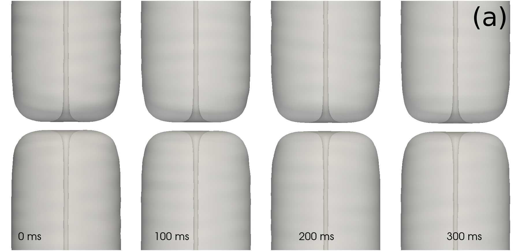
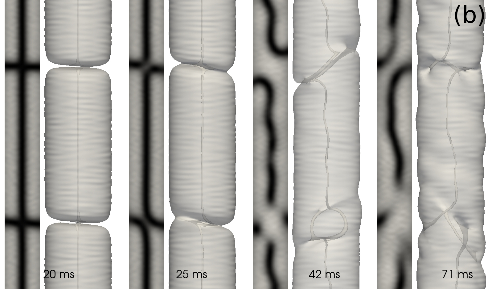
Figure 4: Real time evolution of open vortex lines after adding random perturbations to the corresponding stationary states. (a) Semi-transparent density isocontours at 5 $\%$ of maximum density around the soliton position for a stable state with $\mu=3.0\,\hbar\omega_{\perp}$ and $\omega_{\perp}/2\pi=100$ Hz. (b) Same as (a) for an unstable case containing two solitons, with $\mu=5.1\,\hbar\omega_{\perp}$ and $\omega_{\perp}/2\pi=71.3$ Hz, showing a decay dynamics dominated at early time by the $q=1$ mode (see text). For every time, along with the density isocontour of the whole system on the right, a narrow slice along the $z$-axis shows the density in a greyscale, with vortices in black, on the left.

Bifurcations from the dark soliton state occur if Eqs. (43) have non-trivial solutions for $\omega=0$ Brand2002 ; Mateo2015 . In this case, and for $q=0$ modes, Eqs. (43) are linear Schrödinger equations for $f_{\pm}$, with effective potentials given by $V_{\pm}=V_{\perp}+\hbar^{2}/2mr_{\perp}^{2}+g_{\pm}\psi_{1}^{2}$. In particular, the equation for $f_{-}$ is identical to the GP equation, thus admitting the solution $f_{-}^{G}=\psi_{1}(z,r_{\perp})$, apart from a global phase. This solution is the Goldstone mode associated to the breaking of the continuous symmetry of the phase. Since $f_{-}^{G}$ presents an axial node (the one of the soliton), there must be another solution to Eq. (43) without axial nodes, and then with lower axial energy. This energy difference, associated to the axial degrees of freedom, can be released for the excitation of transverse modes in the condensate, which can produce the decay of the dark soliton. Following a procedure parallel to that used in Ref. Mateo2014 , based in a separable ansatz for $f_{\pm}$ within the Thomas-Fermi regime, the bifurcation points for $q=0$ can be estimated to appear at chemical potential values $\mu_{0}=\sqrt{2}\,({2p+2})\,\hbar\omega_{\perp}$, where $p=1,2,\dots$ is a radial quantum number. The pair $(p,q)$ characterizes the corresponding transverse unstable modes localized at the soliton plane, and indicates the number of radial and azimuthal nodal points, respectively. Specifically, for $(p=1,q=0)$ the predicted unstable mode will appear at $\mu=5.66\,\hbar\omega_{\perp}$, which is close to the value ($\approx 5$) found by numerically solving Eq. (43).

The upper panel of Figure 3 shows the numerical solutions to Eq. (43) for the unstable excitation frequencies of open-vortex-line states. As can be seen, the unstable modes with $q=1,2$ ($p=0$) appear before those with $q=0$. The latter excitations introduce radial nodes ($p\neq 0$) in the soliton plane, whose energy cost is higher than the kinetic energy excess ($\propto\hbar^{2}q^{2}/2m$) of the azimuthal nodes generated by the modes with $q=1,2$. In particular, for a computational domain with periodic boundary conditions and axial length $4\pi\,a_{\perp}$, the excitation of transverse modes with $q=1$ above $\mu=3.0\,\hbar\omega_{\perp}$ marks the threshold for instability. As previously commented, the small bump extended between $3.05\,\hbar\omega_{\perp}$ and $3.4\,\hbar\omega_{\perp}$ on the $\mu$ axis is due to small instabilities derived from the vortex–soliton junction, and are represented by the ($q=1$)–dashed line of Figure 3. To illustrate this point, the lower panel of Figure 3 depicts the density isocontours of an open vortex state with $\mu=\,3.2\,\hbar\omega$ (semi-transparent contour) and its only unstable modes coming from the vortex–soliton junction (colored contours). Such unstable modes are not exclusively localized around the junction. This specific instability ceases to act for an intermediate range of chemical potentials, where the snaking instability makes its appearance through the $q=1$ solid curve.

We have cross-checked our results obtained from the linear stability analysis, by evolving in real time the stationary states $\psi$ with different chemical potentials, after adding a random Gaussian perturbation $\psi\rightarrow\psi+\delta\psi$. The upper panel of Fig. 4 presents an example of such dynamics for a condensate with $\mu=3\,\hbar\omega_{\perp}$, just below the instability threshold. The system remains nearly unaltered during the whole evolution, thus stable according to the linear analysis of Fig. 3; only smooth oscillations due to sound waves can be observed.

For states with two solitons, as shown in Fig.2, whenever the distance between solitons is large in comparison with the healing length, the stability analysis follows that of a single soliton. To illustrate their characteristic dynamics, we have selected an unstable system with $\mu=5.1\,\hbar\omega_{\perp}$, shown in the lower panel of Fig. 4. As can be seen, at about 20 ms, the snaking instability starts to operate at the planes of the solitons, while the vortices begin to lose their alignment. At later time, two new vortices appear as a remainder of the two initial solitons, along with manifest oscillations of the initial straight axisymmetric vortices.

V Half vortex ring states

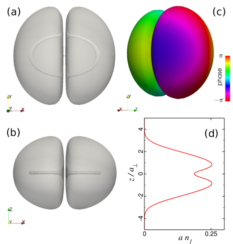
Figure 5: Half vortex rings attached to a dark soliton in an oblate condensate with $\mu=6\,\hbar\omega_{\perp}$ confined by a harmonic trap with aspect ratio $\lambda=1.4$. Density isocontours at 5$\%$ of maximum density are shown for the semi-transparent top and side views (left panels) and the perspective view colored by phase (top right). (d) Column density profile along the $z$-axis.

In this section we consider a variant layout with curved open vortex lines having both ends attached to the same planar dark soliton. The resulting structures bear some resemblance to the U-shaped vortices found in elongated systems Rosenbusch2002 , where the vortex lines bend near their end points. On the contrary, here we focus on half vortex rings. These objects have been studied in the realm of classical fluids Akhmetov2009 , and can propagate long distances attached to the water surface without decaying (see for instance Hu2005 , where they are shown to provide the mechanism of motion for light insects). This configuration mimics an open string whose both ends are attached to the same D-brane, which is another basic configuration of an open string.

In order to generate half vortex rings in a BEC, we proceed with two steps. We first search for stable vortex rings, which are later split into two halves by imprinting a planar dark soliton. To this end, we have chosen near-spherical, harmonically trapped condensates, where the conditions for the stability of vortex rings have been analytically predicted for aspect ratios in the range $1\leq\lambda\leq 2$ within the strongly interacting regime Horng2006 , and have been numerically corroborated in some particular cases near the weakly interacting regime Bisset2015 . Our results show that the analytical prediction breaks down for small values of the chemical potential, where, on the other hand, the conditions for the stability of solitons can be expected. As a result, we have not found a stable half vortex ring, although it is possible to observe robust configurations with weak instabilities. This is the case presented in Fig. 5, corresponding to the aspect ratio $\lambda=1.4$ and the chemical potential $\mu=6\,\hbar\omega_{z}$. The translucent density isocontours Fig. 5(a)-(b) show the condensate from two perpendicular views, and the colored density isocontour Fig. 5(c) reproduces the resulting phase pattern from the interplay between the soliton (lying across the $x$-coordinate) and the vortices. By integration of the density over the $x$-coordinate [panel Fig. 5(d)], it is possible to observe the density depletion produced by the vortices at $z=0$. As demonstrated in Fig. 6(a), showing the real time evolution of this state obtained from the numerical solution of the full GP equation (3), the half vortex ring is a robust state, which is able to survive under perturbations during $100$ ms in a harmonic trap with $\omega_{z}/2\pi=11.5$ Hz.

Other choices of parameters can lead to different lifetimes for half vortex rings. As an alternative example, in Fig. 6(b) we present a near-spherical condensate with $\lambda=1.1$ and a higher chemical potential $\mu=8.9\,\hbar\omega_{z}$, in a trap with $\omega_{z}/2\pi=57.5$ Hz. In this case, the dark soliton decay begins around 10 ms, and the later evolution shows complex dynamics. As a general trend, for high values of $\mu$ we have observed a chaotic scenario at the later stages of the half-vortex-ring decay, including the appearance of new vortex lines that split or reconnect.

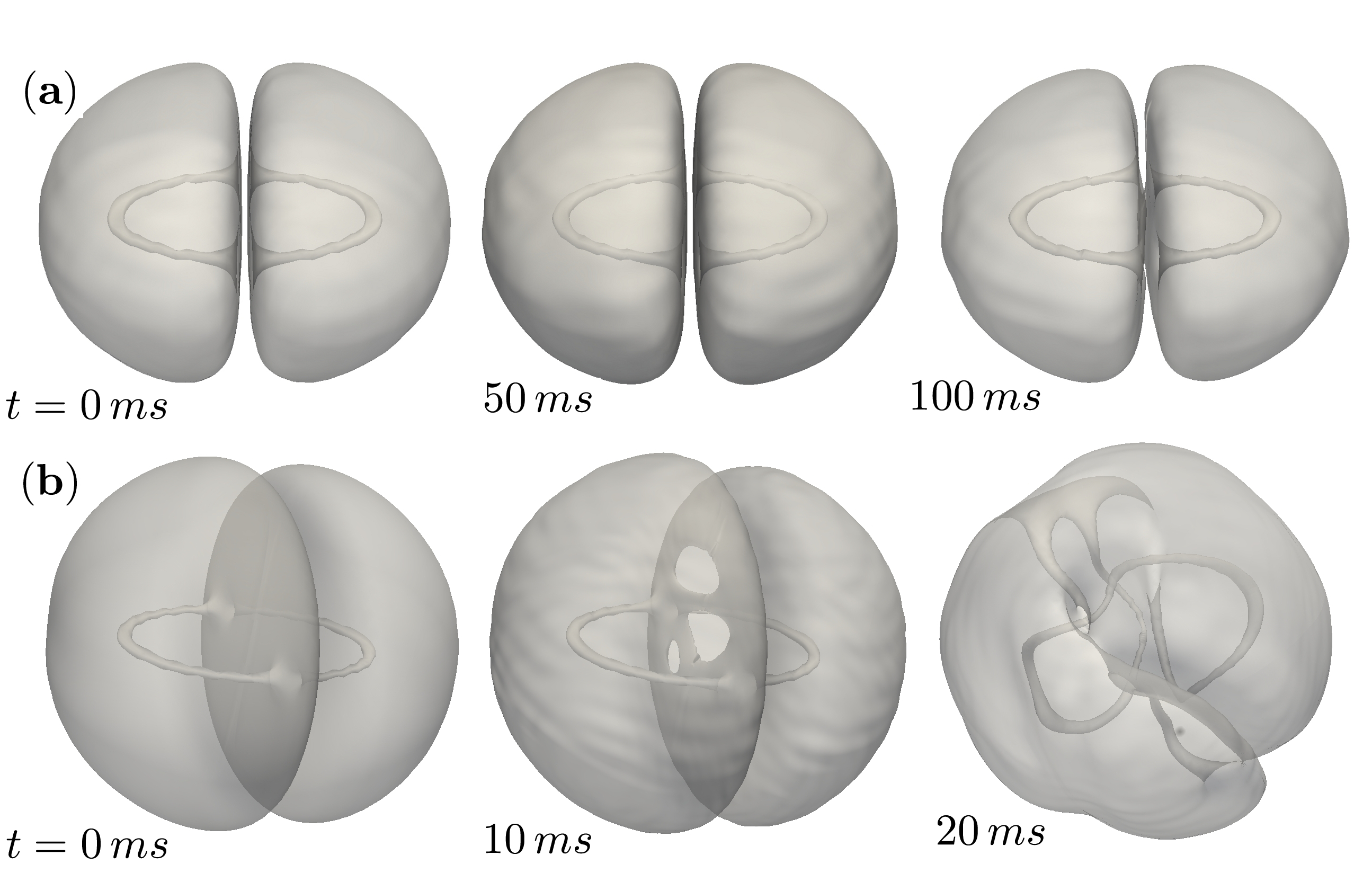
Figure 6: Real time evolution, after adding a random Gaussian perturbation, of half vortex rings in oblate BECs. Semitransparent density isocontours at 5 $\%$ of maximum density are shown at different times for condensates with: (a) $\lambda=1.4$, $\mu=6\,\hbar\omega_{z}$, and $\omega_{z}/2\pi=11.5$ Hz; (b) $\lambda=1.1$, $\mu=8.9\,\hbar\omega_{z}$, and $\omega_{z}/2\pi=57.5$ Hz.

VI Discussion and Conclusions

In this paper two variants of open vortex lines in scalar BECs have been reported, having either one end or two ends of a vortex attached to a planar soliton. In the latter case, consisting of half vortex rings, we have shown that these configurations present long lifetimes for typical parameters of current experiments. For channeled condensates containing straight vortices attached to solitons, we have demonstrated the existence of dynamically stable states and identified the bifurcation points of the first unstable modes. In both variants, a necessary condition for the corresponding configurations to be stationary requires that the vortex lines appear in pairs, as shown in Figs. LABEL:Fig1_os, 2, 4, 5.

The stationary configurations we considered in this paper are either stable (vortex lines attached to planar dark solitons) or long-lived (U-shaped vortex lines), which indicate their feasibility for BEC experimental realizations. To this aim, the well-established experimental techniques in BECs developed for the observation of topological defects, such as optical phase imprinting Burger1999 ; Denschlag2000 or laser stirring Madison2000 , can be used. We propose here two possible ways for elongated condensates adequately devised to prevent the snaking instability Weller2008 . By means of phase imprinting, both a transverse planar soliton and a pinned straight vortex along the $z$-axis could be simultaneously seeded. Alternatively, the laser stirring of the atomic cloud could be applied to drive the condensate into rotation around the $z$-axis, so that an energetically stable, singly charged vortex can be generated. After this, a planar soliton could be imaged onto the condensate by phase imprinting, in order to split the initial vortex into two vortex lines attached to the soliton. With regard to the realization of half vortex rings, the experimental procedures are more elaborate, since they would involve the controlled generation of vortex rings Anderson2001 , within a regime of dynamical stability, followed by the phase imprinting of a soliton. These settings can open up a way to advance in the fairly unexplored domain of the interplay between vortices and solitons.

To summarize, we have demonstrated that stationary, robust states composed of vortex lines attached to planar dark solitons can be found in scalar BECs. Among them, we have reported on dynamically stable configurations in elongated systems for small values of the chemical potential. Our results follow from the Gross-Pitaevskii theory applied to realistic condensates of ultracold gases, and allow the study of vortex lines with Dirichlet boundary conditions. In addition, we have shown that in the hydrodynamic limit the dynamics of open vortex lines can be well characterized by the dual description of the Gross-Pitaevskii theory, which can be viewed as a (3+1)-dimensional effective string theory. This connection might pave the way to test some analytical predictions of string theory with experimental realizations in ultracold gases. To advance in this way, the further analysis of solutions to the equation of motion derived from the string functional Eq. (26) and the comparison with numerical simulations from the Gross-Pitaevskii equation are required, which will be reported elsewhere BECstring3 .

References

- [1] Alexander Fetter. Rotating trapped Bose-Einstein condensates. Reviews of Modern Physics, 81(2):647–691, 2009.
- [2] D. J. Frantzeskakis. Dark solitons in atomic Bose-Einstein condensates: from theory to experiments. J. Phys. A. Math. Gen., 43:213001, 2010.
- [3] A. Schirotzek C. H. Schunck M. W. Zwierlein, J. R. Abo-Shaeer and W. Ketterle. Vortices and superfluidity in a strongly interacting fermi gas. Nature, 435:1047, 2005.
- [4] Mark J. H. Ku, Wenjie Ji, Biswaroop Mukherjee, Elmer Guardado-Sanchez, Lawrence W Cheuk, Tarik Yefsah, and Martin W Zwierlein. Motion of a Solitonic Vortex in the BEC-BCS Crossover. Phys. Rev. Lett., 113:065301, 2014.
- [5] Mark J H Ku, Biswaroop Mukherjee, Tarik Yefsah, and Martin W Zwierlein. From Planar Solitons to Vortex Rings and Lines: Cascade of Solitonic Excitations in a Superfluid Fermi Gas. 2015.
- [6] T.B.W. Kibble. Topology of cosmic domains and strings. J. Phys. A : Math. Gen., 9(8), 1976.
- [7] W. H. Zurek. Cosmological experiments in superfluid helium? Nature, 317(505), 1985.
- [8] Giacomo Lamporesi, Simone Donadello, Simone Serafini, Franco Dalfovo, and Gabriele Ferrari. Spontaneous creation of Kibble–Zurek solitons in a Bose–Einstein condensate. Nat. Phys., 9(10):656–660, 2013.
- [9] C. M. Savage and J. Ruostekoski. Dirac monopoles and dipoles in ferromagnetic spinor Bose-Einstein condensates. Phys. Rev. A, (68):043604, 2003.
- [10] Magnus O. Borgh and Janne Ruostekoski. Topological Interface Engineering and Defect Crossing in Ultracold Atomic Gases. Phys. Rev. Lett., (109):015302, 2012.
- [11] D I Bradley, S N Fisher, A M Gu Eacute Nault, R P Haley, J Kopu, H Martin, G R Pickett, J E Roberts, and V Tsepelin. Relic topological defects from brane annihilation simulated in superfluid 3He. Nature Physics, 4(1):46, 2007.
- [12] Kenichi Kasamatsu, Hiromitsu Takeuchi, Muneto Nitta, and Makoto Tsubota. Analogues of D-branes in Bose-Einstein condensates. JHEP, 11:068, 2010.
- [13] Kenichi Kasamatsu, Hiromitsu Takeuchi, and Muneto Nitta. D-brane solitons and boojums in field theory and Bose-Einstein condensates. J. Phys. Condens. Matter, 25:404213, 2013.
- [14] Kenichi Kasamatsu, Hiromitsu Takeuchi, Makoto Tsubota, and Muneto Nitta. Wall-vortex composite solitons in two-component bose-einstein condensates. Phys. Rev. A, 88:013620, 2013.
- [15] M. W. Ray, E. Ruokokoski, K. Tiurev, M. Möttönen, and D. S. Hall. Observation of isolated monopoles in a quantum field. Science, 348(6234):544–547, 2015.
- [16] M. W. Ray, E. Ruokokoski, S. Kandel, M. Möttönen, and D. S. Hall. Observation of Dirac monopoles in a synthetic magnetic field. Nature (London), 505:657–660, January 2014.
- [17] A. Muñoz Mateo and V. Delgado. Effective equations for matter-wave gap solitons in higher-order transversal states. Physical Review E, 88:042916, 2013.
- [18] Fernando Lund and Tullio Regge. Unified approach to strings and vortices with soliton solutions. Phys. Rev. D, 14:1524–1535, Sep 1976.
- [19] A. Zee. Vortex strings and the antisymmetric gauge potential. Nucl.Phys., B421:111–124.
- [20] Steven S. Gubser, Revant Nayar, and Sarthak Parikh. Strings, vortex rings, and modes of instability. Nucl. Phys., B892:156–180, 2015.
- [21] Steven S. Gubser, Bart Horn, and Sarthak Parikh. Perturbations of vortex ring pairs. Phys. Rev. D, 93:046001, Feb 2016.
- [22] Bart Horn, Alberto Nicolis, and Riccardo Penco. Effective string theory for vortex lines in fluids and superfluids. Journal of High Energy Physics, 2015(10):1–58, 2015.
- [23] M. Franz. Vortex-boson duality in four space-time dimensions. Europhys. Lett., 77:47005, 2007.
- [24] Stefano Giaccari and Jun Nian. Dark Solitons, D-branes and Noncommutative Tachyon Field Theory. 2016.
- [25] J. Hubbard. Calculation of partition functions. Phys. Rev. Lett., 3:77–78, Jul 1959.
- [26] B. Zwiebach. A first course in string theory. Cambridge University Press, 2006.
- [27] Vladimir V. Konotop and Lev Pitaevskii. Landau Dynamics of a Grey Soliton in a Trapped Condensate. Physical Review Letters, 93:240403, 2004.
- [28] Ahmed Abouelsaood, Curtis G. Callan, Jr., C. R. Nappi, and S. A. Yost. Open Strings in Background Gauge Fields. Nucl. Phys., B280:599–624, 1987.
- [29] A. Muñoz Mateo and J Brand. Chladni Solitons and the Onset of the Snaking Instability for Dark Solitons in Confined Superfluids. Phys. Rev. Lett., 113(25):255302, 2014.
- [30] EA Kuznetsov and SK Turitsyn. Instability and collapse of solitons in media with a defocusing nonlinearity. Sov. Phys. JETP, 67(August 1988):1583–1588, 1988.
- [31] Joachim Brand and William P. Reinhardt. Solitonic vortices and the fundamental modes of the “snake instability”: Possibility of observation in the gaseous Bose-Einstein condensate. Phys. Rev. A, 65:043612, 2002.
- [32] A. Muñoz Mateo and J Brand. Stability and dispersion relations of three-dimensional solitary waves in trapped Bose–Einstein condensates. New J. Phys., (17):125013, 2015.
- [33] V. Bretin P. Rosenbusch and J. Dalibard. Dynamics of a single vortex line in a bose-einstein condensate. Phys. Rev. Lett., 89:200403, 2002.
- [34] D. G. Akhmetov. Vortex rings. Springer, 2009.
- [35] David L. Hu and John W. M. Bush. Meniscus-climbing insects. Nature, 437(7059):733–736, 2005.
- [36] T.-L. Horng, S.-C. Gou, and T.-C. Lin. Bending-wave instability of a vortex ring in a trapped Bose-Einstein condensate. Phys. Rev. A, 74(4):041603, 2006.
- [37] C. Ticknor R. Carretero-González D. J. Frantzeskakis L. A. Collins R. N. Bisset, W. Wang and P. G. Kevrekidis. Bifurcation and stability of single and multiple vortex rings in three-dimensional bose-einstein condensates. Phys. Rev. A, 92(043601), 2015.
- [38] S. Burger, K. Bongs, S. Dettmer, W. Ertmer, K. Sengstock, A. Sanpera, G. V. Shlyapnikov, and M. Lewenstein. Dark Solitons in Bose-Einstein Condensates. Phys. Rev. Lett., 83(25):5198–5201, 1999.
- [39] J Denschlag, Je E Simsarian, Dl L Feder, Cw Charles W Clark, La A Collins, J Cubizolles, L Deng, Ew W Hagley, K Helmerson, Wp William P Reinhardt, Sl L Rolston, Bi I Schneider, and Wd William D Phillips. Generating solitons by phase engineering of a bose-einstein condensate. Science (New York, N.Y.), 287(5450):97–101, 2000.
- [40] K.W. Madison, F. Chevy, and W. Wohlleben. Vortex formation in a stirred Bose-Einstein condensate. Physical review letters, 84(5):806–809, 2000.
- [41] A. Weller, J. P. Ronzheimer, C. Gross, J. Esteve, M. K. Oberthaler, D. J. Frantzeskakis, G. Theocharis, and P. G. Kevrekidis. Experimental observation of oscillating and interacting matter wave dark solitons. Phys. Rev. Lett., 101:130401, 2008.
- [42] B. P. Anderson, P. C. Haljan, C. A. Regal, D. L. Feder, L. A. Collins, C. W. Clark, and E. A. Cornell. Watching Dark Solitons Decay into Vortex Rings in a Bose-Einstein Condensate. Phys. Rev. Lett., 86(14):2926–2929, 2001.
- [43] A. Muñoz Mateo, Xiaoquan Yu, and Jun Nian. unpublished.