Collective resonance fluorescence in small and dense atom clouds:
Comparison between theory and experiment

Abstract

We study the emergence of a collective optical response of a cold and dense ⁸⁷Rb atomic cloud to a near-resonant low-intensity light when the atom number is gradually increased. Experimental observations are compared with microscopic stochastic simulations of recurrent scattering processes between the atoms that incorporate the atomic multilevel structure and the optical measurement setup. We analyze the optical response of an inhomogeneously-broadened gas and find that the experimental observations of the resonance line shifts and the total collected scattered light intensity in cold atom clouds substantially deviate from those of thermal atomic ensembles, indicating strong light-induced resonant dipole-dipole interactions between the atoms. At high densities, the simulations also predict a significantly slower decay of light-induced excitations in cold than in thermal atom clouds. The role of dipole-dipole interactions is discussed in terms of resonant coupling examples and the collective radiative excitation eigenmodes of the system.

I Introduction

An improved experimental control of cold atoms and an increase in computing power now allow both measurements and many-body simulations of the optical response in small atomic ensembles. These systems have proved to be important since strong light-induced dipole-dipole (DD) interactions can lead to collective light scattering phenomena. In particular, it was recently pointed out Javanainen et al. (2014) that a cold and dense atomic medium can exhibit light-induced correlations and an optical response that dramatically differ from those of a thermal, inhomogeneously-broadened medium.

Here we analyze in detail near-resonance light scattering from small clouds of cold or thermal, trapped ⁸⁷Rb atoms that were recently experimentally measured or numerically simulated in Refs. Pellegrino et al. (2014); Jenkins et al. (2016). Large-scale numerical classical electrodynamic simulations and experimental observations indicate the emergence of collective effects in the optical response of a cold-atom sample due to DD interactions, as the number of atoms is gradually increased and the density of the cloud increases. The experimentally observed light scattering and classical electrodynamic simulations provide a detailed side-by-side comparison between experiment and theory in a gas of multilevel ⁸⁷Rb atoms. By performing microscopic numerical simulations of both cold and hot atomic ensembles, in which the atoms are represented by linear point emitters in the low excitation limit, we find that the experimental observations of the resonance line shifts and the total collected scattered light intensity substantially deviate from those of thermal atomic ensembles. In particular, in both cases the density-dependent resonance shift is absent. However, introducing inhomogeneous broadening due to thermal atomic motion restores the shift.

The experiments are performed in a microscopic elongated dipole trap where we study the role of DD interactions between ⁸⁷Rb atoms in the resonance fluorescence by varying the atom number from one to $\sim 450$. The sample is illuminated by near-resonant low-intensity laser pulses. Before the illumination the atoms are laser-cooled to a temperature $\sim 110\mu$K, such that the thermal Doppler broadening is negligible. The corresponding stochastic simulations go beyond idealized models, by incorporating a nonuniform atom density, the effects of an anisotropic elongated trap, the multilevel structure of the $F=2$ ground-state manifold of ⁸⁷Rb, imaging geometry, and the optical components such as lenses and polarizers. In the simulations the thermally-induced broadening of hot atoms is generated by stochastically sampling the inhomogeneous broadening of the resonance frequencies of individual atoms. The numerical simulations also incorporate the recurrent (dependent) scattering processes between the atoms where the light is scattered more than once by the same atom. These are the source of light-induced correlations between the atoms Javanainen et al. (2014); Ruostekoski and Javanainen (1997a). We find that the strong DD interactions in the system lead to collective excitation eigenmodes of the system that exhibit a broad range of collective radiative linewidths. The role of collective eigenmodes is revealed in the temporal profile of the decay of light-induced excitations after the incident laser pulse is switched off. For large atom numbers in stochastic simulations we find a significantly slower decay of the excitations for cold than for thermal atom clouds.

The radiative interactions in ensembles of resonant emitters constitute an active area of research that covers a variety of systems, such as thin thermal atom cells Keaveney et al. (2012), metamaterial arrays of nanofabricated resonators Lemoult et al. (2010); Fedotov et al. (2010); Adamo et al. (2012); Jenkins and Ruostekoski (2013), arrays of ions Meir et al. (2014), and nanoemitters Brandes (2005); Pierrat and Carminati (2010). Experiments in cold atomic ensembles have dominantly addressed optically thick but relatively dilute samples Balik et al. (2013); Bienaimé et al. (2010); Löw et al. (2005); Kwong et al. (2014, 2015); Bromley et al. (2016); Guerin et al. (2016a); Bons et al. (2016); Roof et al. (2016); Araújo et al. (2016), whereas the setup described here deals with small samples but at higher densities. It has been used to study fluorescence Pellegrino et al. (2014); Jenkins et al. (2016) and forward scattering Jennewein et al. (2016, 2015), although the present paper concentrates on the case of fluorescence. Theoretically, ensembles of resonant emitters provide a rich and challenging phenomenology whereby light-induced correlation effects Dicke (1954); Lehmberg (1970a, b); Saunders and Bullough (1973); Ishimaru (1978); van Tiggelen et al. (1990); Morice et al. (1995); Ruostekoski and Javanainen (1997a, b); Rusek et al. (1996); Javanainen et al. (1999); Ruostekoski and Javanainen (1999); Berhane and Kennedy (2000); Clemens et al. (2003); Chomaz et al. (2012); Jenkins and Ruostekoski (2012a, b); Olmos et al. (2013); Antezza and Castin (2013); Javanainen et al. (2014); Pellegrino et al. (2014); Javanainen and Ruostekoski (2016); Kuraptsev and Sokolov (2014); Skipetrov and Sokolov (2014); Bettles et al. (2015); Lee et al. (2016); Bettles et al. (2016); Schilder et al. (2015); Longo et al. (2016); Sutherland and Robicheaux (2016); Jones et al. (2016); Syzranov et al. (2015); Guerin et al. (2016b); Zhu et al. (2016) due to recurrent scattering can profoundly alter the optical response of sufficiently dense samples.

Parallel to our work, the effects of motional dynamics of atoms were observed in a cold Sr atom vapor by comparing the optical response of narrow and broad linewidth transitions of the atoms Bromley et al. (2016). A qualitatively different behavior was observed in the two cases. Unlike our experiment, Ref. Bromley et al. (2016) considered a dilute gas $\rho/k^{3}\sim 10^{-3}$. Another important difference is that the narrow Sr resonance is affected by the recoil shift of the atom.

We begin with a brief overview of the experimental setup in Sec. II. This is followed by a description of strong DD interactions in cold and dense atomic ensembles in Sec. III. We first cover the simple case of a two-level atom and how to incorporate the effects of inhomogeneous broadening. The discussion is then extended to the multilevel ⁸⁷Rb case in Sec. III.2. We present the experimental and numerical results in Sec. IV by first analyzing the collective modes and their decay in Sec. IV.1, then the experimental observations in Sec. IV.2, and the theoretical results in Sec. IV.3. Finally, some concluding remarks are made in Sec. V.

II Experimental Setup

As described in Ref Pellegrino et al. (2014), our experimental setup enables us to access densities and temperatures at which strong DD interactions manifest themselves in the optical response. To achieve this, we laser-cool an ensemble of $N$ ⁸⁷Rb atoms in a microscopic dipole trap obtained by focusing a laser beam with a wavelength of 957 nm onto a spot size of 1.6 $\mu$m, as depicted in Fig. 1(a). We obtain an elongated cloud at a temperature of $\sim 110\,\mathrm{\mu K}$ Bourgain et al. (2013), with a thermal Gaussian distribution with root-mean-square sizes of $\sigma_{x}=\sigma_{y}=0.3\lambda$ and $\sigma_{z}=2.4\lambda$, where $\lambda\simeq 780.2\,\mathrm{nm}$ is the resonant wavelength of the D2 transition used in this work. Varying the number of atoms in the trap from $N=1$ to $N=450$ allows us to study the increasing role of inter-atomic interactions in the radiative response. For the largest atom numbers the peak density at the center of the trap is $\rho\simeq 0.9k^{3}$ ($k\equiv 2\pi/\lambda$), which, as we show in Sec. III, results in DD interactions strong enough to heavily influence the optical response of the atomic cloud. At the same time, thermal motion within this cold atomic cloud produces only a negligible Doppler broadening of $0.04\gamma$, where $\gamma=2\pi\times 3\,\mathrm{MHz}$ is the half width half maximum (HWHM) radiative linewidth of the D2 transition

$$\gamma=\frac{{\cal D}^{2}k^{3}}{6\pi\hbar\epsilon_{0}}\,,$$ (1)

where ${\cal D}$ denotes the reduced dipole matrix element. The number of atoms $N$ is experimentally controlled with a 10% uncertainty. The uncertainties in the temperature, atom number, and the waist size lead to an uncertainty on the peak atom density of a factor of two.

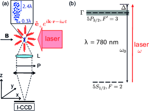
Figure 1: (a) Experimental setup. The atoms are initially confined in a microscopic single-beam dipole trap (not shown) (wavelength $957$ nm, depth $1$ mK, and waist $1.6$ $\mu$m, oscillation frequencies $\omega_{x}=\omega_{y}=2\pi\times 62$ kHz and $\omega_{z}=2\pi\times 8$ kHz). The excitation laser propagates anti-parallel to the quantization axis $x$, set by a magnetic field $B\sim 1$ G. We collect light scattered in the negative $z$ direction, after a polarizer $P$ oriented at an angle of $55^{\circ}$ with respect to $x$, using a lens $L$ with a large numerical aperture ($\textrm{NA}=0.5$) and an image intensifier followed by a CCD camera (I-CCD). (b) Structure of ⁸⁷Rb atoms relevant to this work. The excitation light at frequency $\omega$ is near resonant with the transition at $\lambda=2\pi/\omega_{0}=780\,\mathrm{nm}$.

We observe the light scattered by the cloud when it is illuminated by an incident laser field tuned near the resonance of the transition between ground and excited hyperfine levels $|g\rangle=(5S_{1/2},F=2)$ and $|e\rangle=(5P_{3/2},F^{\prime}=3)$, respectively; Fig. 1(b). The incident field is sent along the small axis of the cloud and has a $\sigma_{+}$ polarization, where we use the unconventional unit vectors,

$$\hat{\mathbf{e}}_{\pm 1}=\mp{1\over\sqrt{2}}(\hat{\mathbf{e}}_{y}\pm i\hat{\mathbf{e}}_{z}),\quad\hat{\mathbf{e}}_{0}=\hat{\mathbf{e}}_{x}\,,$$ (2)

corresponding to the labeling of the directions in the experiment, shown in Fig. 1(a), with the $x$ axis as the quantization axis set by a 1 Gauss magnetic field.

Prior to the illumination by the excitation laser, we prepare the atoms in the hyperfine ground level $|g\rangle$ with $95\%$ efficiency using a $\sigma_{+}$-polarized beam tuned on the $(5S_{1/2},F=1)$ to $(5P_{3/2},F^{\prime}=2)$ transition. The atoms are thus prepared in an incoherent mixture of Zeeman states $\left|g,m\right\rangle$ ($|m|\leq 2$) with relative populations $p_{m}$, estimated by solving rate equations:

$$p_{-2}=p_{-1}\simeq 0,\quad p_{0}=p_{1}=p_{2}\simeq 1/3\,.$$ (3)

In the experiments reported in Sec. IV.2 we use flat-top light pulses to excite the prepared atoms, with durations ranging from $T=125\,\mathrm{ns}$ (rise time $\sim 7$ ns, using an electro-optical modulator) to $T=2$ $\mu$s (rise time $\sim 50$ ns, using an acousto-optical modulator). We employ pulses with low intensity $I<0.1I_{\rm sat}$ ($I_{\rm sat}=1.6\,\mathrm{mW/cm^{2}})$ in order to operate in the limit where the response of the atoms to light is linear. The probe frequency is $\omega=\omega_{0}+\Delta$, where $\omega_{0}$ is the resonance frequency of the $|g\rangle\leftrightarrow|e\rangle$ transition in the absence of a magnetic field.

III The influence of DD interactions on the optical response

An incident field nearly resonant with the $|g\rangle\leftrightarrow|e\rangle$ transition induces electric dipoles in each of the atoms. In this Section, we will see how interactions between the dipoles bring about a collective response of the gas in response to the incident field. The key here is that each atom is driven not only by the incident field, but also by the fields emitted by all other atoms in the gas. The resulting DD interactions profoundly alter the cloud’s scattering properties at atom densities attained in our experiments.

Generally, in the limit of low light intensity, recurrent scattering, in which a photon repeatedly scatters between the same atoms, results in dynamics where a cloud’s polarization density depends on two-body correlations involving the polarization density and the atomic number density Ruostekoski and Javanainen (1997a). These two-body correlations depend on three-body correlations, which depend on four body-correlations, and so on. To exactly account for the DD interactions in the optical response of an $N$-body system, one would ultimately need to solve the dynamics of $N$-body correlation functions.

Fortunately, in the limit of low light intensity one can avoid the coupled equations of the correlation functions by carrying out a stochastic simulation instead Javanainen et al. (1999); Lee et al. (2016). We first sample stochastically $N$ atomic positions $\{\mathbf{X}_{1},\ldots,\mathbf{X}_{N}\}$ from the joint probability distribution of the positions. In our experiment, at temperatures of $110\,\mathrm{\mu{}K}$, the de Broglie wavelength is much smaller than the inter-atomic separation. We therefore treat the atomic positions in our harmonic trap as independent identically distributed Gaussian random variables with the experimentally observed root-mean-square widths $\sigma_{x}=\sigma_{y}=0.3\lambda$ and $\sigma_{z}=2.4\lambda$. The atom at each position $\mathbf{X}_{j}$ is taken to be a linear dipole driven by the electric field falling on it. We next solve the optical response for such a collection of dipoles and compute the relevant observable(s). To model an experiment, real or hypothetical, we finally average the result(s) over a large number of samples of atomic positions. In the simulations we consider both the steady-state and time-dependent cases.

For each atomic sample, the optical response may be analyzed in terms of collective dipole excitations, each with a distinct resonance frequency and decay rate. The cooperative nature of a cloud’s response can be roughly characterized by the widths of the distributions of collective resonance shifts and decay rates. We will show that at the densities reached in the experiment, the interactions between an atom and its nearest neighbor sensitively depend on their relative distance, thus illustrating the role of DD interactions in the formation of correlations in the cold atoms.

We will then review how this model can be generalized to a cloud of ⁸⁷Rb atoms, accounting for Zeeman degeneracy Pellegrino et al. (2014), in Sec. III.2. In the case of multiple electronic ground states the simulations represent a classical approximation where the recurrent scattering between the atoms is included, but nonclassical higher order correlations between internal levels that involve fluctuations between ground-state coherences of different levels and the polarization are factorized Lee et al. (2016). In the limit of low light intensity (that we assume everywhere in this paper) the classical approximation correctly represents all the atomic ground-state population expectation values of even the exact quantum solution.

We will illustrate that, in a cloud of $N=450$ atoms as realized in the experiment, the light-induced DD interactions between the atoms result in broad distributions of collective mode resonance frequencies and decay rates. We will also discuss the effects of atomic motion in a thermal sample by introducing an inhomogeneous broadening to the resonance frequencies of the atoms, but still considering the atoms as frozen during their interaction with the probe light.

III.1 Coupled dynamics of two-level atoms

For simplicity we introduce the theoretical model first by considering an ensemble of two-level atoms, before generalizing to the multilevel scheme that describes the ⁸⁷Rb $F=2$ ground-state experiments. Since the vectorial nature of electric field and dipole moment matters in this paper, the two-level atom is assumed to have the vector dipole moment matrix element between the ground and excited state ${\cal D}\hat{\mathbf{{e}}}$, where ${\cal D}$ is real and $\hat{\mathbf{{e}}}$ is a possibly complex unit vector. This situation could be approximated experimentally by applying a strong magnetic field on an atom, so that only one transition between the Zeeman levels is close to resonance with the driving light.

III.1.1 Basic relations

For each stochastic realization of atomic positions, we have an ensemble of $N$ atoms with ground state $\left|g\right\rangle$ and excited state $\left|e\right\rangle$, which the incident field couples via an electric dipole transition with resonance frequency $\omega_{0}$. In the low-intensity limit, in which population of the excited state can be neglected, the expected scattered field can be computed by treating the atoms as classical linear oscillators whose dipole moments are given by

$$\mathbf{d}_{j}(t)=\hat{\mathbf{{e}}}\,{\cal D}\mathcal{P}^{(j)}(t)\textrm{.}$$ (4)

When analyzing the light and atoms, we adopt the rotating wave approximation where the dynamics is dominated by the frequency of the driving laser $\omega$. Here, and in the rest of the paper, the light and atomic field amplitudes refer to the slowly-varying versions of the positive frequency components of the corresponding variables, where the rapid oscillations $e^{-i\omega t}$ due to the laser frequency have been factored out. In Eq. (4) $\mathcal{P}^{(j)}$ is a dimensionless dipole amplitude; the index $j=1,\ldots,N$ denotes the $j^{\rm th}$ atom with the position $\mathbf{X}_{j}$. This dipole, in turn, emits an electric field with the amplitude

$$\epsilon_{0}\mathbf{E}_{S}^{(j)}({\bf r})=\mathsf{G}({\bf r}-\mathbf{X}_{j})\hat{\mathbf{{e}}}\,{\cal D}\mathcal{P}^{(j)}\textrm{,}$$ (5)

where $\mathsf{G}$ is the monochromatic dipole radiation kernel whose elements are given in Cartesian coordinates by Zangwill (2013)

$$\mathsf{G}_{ij}(\mathbf{r})=\left[\frac{\partial}{\partial r_{i}}\frac{\partial}{\partial r_{j}}-\delta_{ij}\nabla^{2}\right]\frac{e^{ikr}}{4\pi r}-\delta_{ij}\delta({\bf r})\textrm{ .}$$ (6)

There is a characteristic length to the dipole radiation set by the wave number of the light, $k^{-1}=\lambda/2\pi$.

An incident field with $\boldsymbol{\mathbf{\cal E}}_{0}(\mathbf{r},t)$ drives the atomic sample. The atom $j$ in the ensemble is driven by the electric field that includes the incident field and the fields emitted by all other atoms in the system,

$$\mathbf{E}_{\rm ext}(\mathbf{X}_{j},t)=\boldsymbol{\mathbf{\cal E}}_{0}({\mathbf{X}_{j}},t)+\sum_{l\neq j}\mathbf{E}_{S}^{(l)}(\mathbf{X}_{j},t).$$ (7)

This results in the atomic dipole amplitudes satisfying the coupled dynamics

$$\frac{d}{dt}\mathcal{P}^{(j)}=\left(i\Delta-\gamma\right)\mathcal{P}^{(j)}+i\frac{\xi}{{\cal D}}\hat{\mathbf{{e}}}^{\ast}\cdot\epsilon_{0}\mathbf{E}_{\rm ext}(\mathbf{X}_{j})\textrm{,}$$

$$=\left(i\Delta-\gamma\right)\mathcal{P}^{(j)}+i\xi\sum_{l\neq j}{\cal G}^{(jl)}\mathcal{P}^{(l)}+i\frac{\xi}{{\cal D}}\hat{\mathbf{{e}}}^{\ast}\cdot\epsilon_{0}\boldsymbol{\mathbf{\cal E}}_{0}(\mathbf{X}_{j}),$$

with the detuning $\Delta=\omega-\omega_{0}$, the single-atom Wigner-Weisskopf linewidth $\gamma$ [Eq. (1)], and

$$\xi={6\pi\gamma\over k^{3}}\,.$$ (9)

${\cal G}^{(jl)}$ is the DD coupling between two different atoms $j$ and $l$,

$$\mathcal{G}^{(jl)}=\hat{\mathbf{{e}}}^{\ast}\cdot\mathsf{G}(\mathbf{X}_{j}-\mathbf{X}_{l})\hat{\mathbf{{e}}}\textrm{.}$$ (10)

The decay rate $\gamma$ may, in fact, be regarded as a result of the dipolar field acting back on the same atom that radiates it.

In typical situations we are mostly interested in the steady-state response. It is then useful to introduce the atomic polarizability $\alpha=-{\cal D}^{2}/[\hbar\epsilon_{0}(\Delta+i\gamma)]$ that provides the relationship between the atomic dipole amplitude and the field driving the atom

$${\cal D}\mathcal{P}^{(j)}=\alpha\epsilon_{0}\,\hat{\mathbf{{e}}}^{\ast}\cdot\mathbf{E}_{\rm ext}(\mathbf{X}_{j})\,.$$ (11)

This simulation procedure with coupled dipoles accounts for recurrent scattering of light between the atoms to all orders, exactly reproducing the dynamics of light-induced $N$-body correlation functions for stationary atoms in the limit of low light intensity, and was originally introduced for atomic systems in Ref. Javanainen et al. (1999) (see also Lee et al. (2016)); owing to the simple level structure and the low light intensity, the coupled-dipole model simulations are exact even in quantum mechanics Javanainen et al. (1999); Lee et al. (2016). The close correspondence between the classical electrodynamics and the quantum-mechanical collective emission of a single-photon excitation for a cloud of $N$ two-level atoms was also discussed in Ref. Svidzinsky et al. (2010).

The coupled equations for the dipole amplitudes (III.1.1) are linear, of the form

$$\dot{\mathrm{b}}=-i\mathcal{H}\mathrm{b}+\mathrm{F}\textrm{,}$$ (12)

where $\mathrm{b}$ is a vector made of the amplitudes $\mathcal{P}^{(j)}$, say, $\mathrm{b}=[\mathcal{P}^{(1)},\ldots,\mathcal{P}^{(N)}]^{\rm T}$, $-i\mathcal{H}$ is the coupling matrix corresponding to the first two terms on the right-hand side of Eq. (III.1.1), and $\mathrm{F}$ is a vector whose components correspond to the driving of the dipoles by the incident field.

The evolution of the coupled atom-light system can be analyzed using collective eigenmodes $n$ ($n=1,\ldots,N$), which correspond to the eigenvectors $\mathrm{v}_{n}$ of $\mathcal{H}$ with the eigenvalues $\delta_{n}-i\upsilon_{n}$. Here $\delta_{n}$ is the difference between the collective mode resonance frequency and the resonance frequency of a single, isolated atom, and $\upsilon_{n}$ is the collective radiative linewidth. The matrix $\mathcal{H}$ is in general not Hermitian, hence the nonzero imaginary parts of the eigenvalues. Moreover, the eigenvectors are not necessarily orthogonal. In all of our examples, though, they still form a basis. One can therefore uniquely express the dipole amplitudes and the driving incident field as

$$\mathrm{b}(t)=\sum_{n}c_{n}(t)\mathrm{v}_{n},\quad\mathrm{F}(t)=\sum_{n}f_{n}(t)\mathrm{v}_{n}.$$ (13)

Conversely, given $\mathrm{b}$ at any time $t$, the first of Eqs. (13) may be construed as a linear set of equations from which to solve the coefficients $c_{n}$, and likewise for the second equation.

From Eq. (12), the amplitudes $c_{n}$ of the collective mode (here driven at the single atom resonance) satisfy the equation of motion

$$\dot{c}_{n}=\left(-i\delta_{n}-\upsilon_{n}\right)c_{n}+f_{n}(t)\,\textrm{.}$$ (14)

Equivalently, since the atoms are not excited before the incident field is turned on [$c_{n}(-\infty)=0$], the amplitudes satisfy

$$c_{n}(t)=\int_{-\infty}^{t}dt^{\prime}e^{\left(-i\delta_{n}-\upsilon_{n}\right)\left(t-t^{\prime}\right)}f_{n}(t^{\prime})\,\textrm{.}$$ (15)

This is how we handle explicitly time-dependent excitation pulses in the present paper.

For a driving field that is turned on at time $t=0$ and remains constant in time, the inverse of the collective linewidth $1/\upsilon_{n}$ is a measure of how quickly a collective mode will reach its steady state. In the special case of a driving field with a time-independent amplitude and hence constant $f_{n}$, the atomic response eventually reaches a steady state. In the present notation the steady state is specified by

$$c_{n}=\frac{f_{n}}{i\delta_{n}+\upsilon_{n}}.$$ (16)

The same steady state could be found directly from Eq. (12) by solving the linear set of equations $-i\mathcal{H}\mathrm{b}+\mathrm{F}=0$ for the excitation amplitudes $\mathrm{b}$.

Given the vector of the dipole excitations $\mathrm{b}$, one can compute the electric field at an arbitrary position ${\bf r}$, except for the exact positions of the atoms, from

$$\mathbf{E}({\bf r},t)=\boldsymbol{\mathbf{\cal E}}_{0}({\bf r},t)+\sum_{l}\mathbf{E}_{S}^{(l)}({\bf r},t).$$ (17)

Of course, the assumption here and in all of our development is that the slowly varying quantities do not change substantially during the time it takes light to propagate across the atomic sample. That is why the time argument, explicit or implied, is the same throughout our equations. The assumption is valid in light propagation, provided that the group velocity of light does not become comparable with $L\gamma$ where $L$ denotes the characteristic sample size.

III.1.2 Inhomogeneous broadening

At the very low temperatures of the experiments the atoms make a homogeneously broadened sample; to the leading order of approximation they do not move at all. We have thus adopted a “frozen gas” approximation with stationary atoms. In principle one could allow the atoms to move ballistically and in response to the dipole forces between the atoms, even take into account collisions of other origin, and integrate the equations of the polarization amplitudes (III.1.1) treating the positions $\mathbf{X}_{j}$ as time dependent. This would make the propagation phases such as $e^{ikr}$ in the dipolar field time dependent, and bring in the usual consequences of the atomic motion such as the Doppler shifts. The drawbacks are that then both our analysis of the collective modes and the notion of a microscopic stationary state break down, and the management of the motion in and of itself greatly complicates the coding.

Instead, we resort to a simple model of inhomogeneous broadening. Although our aim here is to model the Doppler shifts of moving atoms Javanainen et al. (2014), the simulation procedure for the inhomogeneous broadening is general and applies also to other resonant emitter systems Jenkins and Ruostekoski (2012c), such as those consisting of circuit resonators or quantum dots in which case typical sources for inhomogeneous broadening are fabrication imperfections.

In order to incorporate the inhomogeneous broadening to the stochastic model we add to the detuning of the $j^{\rm th}$ atom a random quantity $\zeta_{j}$ that has a Gaussian distribution with the root-mean-square width $\Omega$. For instance, with $\Omega=ku$ and $u=\sqrt{k_{B}T/m}$ being the thermal velocity, this would be the standard model for the Doppler broadening of a resonance line of an atom with mass $m$ at the temperature $T$. Instead of the usual Lorentzian resonance line of width $\gamma$ (normalized here to the maximum value of one), we use the Voigt profile (the convolution of a Lorentzian and a Gaussian):

$$V(\Delta,\gamma,\Omega) =\frac{1}{\sqrt{2\pi}\,\Omega}\int d\zeta\frac{\gamma^{2}}{(\Delta+\zeta)^{2}+\gamma^{2}}e^{-\frac{\zeta^{2}}{2\Omega^{2}}}$$

$$= \sqrt{\frac{\pi}{2}}\frac{\gamma}{\Omega}\Re\left[e^{\frac{(\gamma-i\Delta)^{2}}{2\Omega^{2}}}\text{erfc}\left(\frac{\gamma-i\Delta}{\sqrt{2}\,\Omega}\right)\right],$$ (18)

where erfc stands for the complement of the error function. We then fit $A\,V(\Delta-\delta\omega,\gamma,\Omega)$ to a resonance line, with any of $A$, $\delta\omega$, $\gamma$ or $\Omega$ regarded as variable parameters as needed, providing an estimate of the resonance shift $\delta\omega$ of the sample from the atomic resonance $\omega_{0}$.

III.1.3 General role of DD interactions

To appreciate qualitatively the effect that the DD interactions have on the atomic response, we display in Fig. 2 the distribution of nearest-neighbor separations in an atomic gas of $N=450$ atoms corresponding to the experimental setup. The interatomic separation distance $1/k$ that represents the characteristic length scale associated with the dipole radiation and below which the light-induced DD interactions become especially strong is highlighted in the plot.

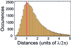
Figure 2: Stochastic simulation of the probability distribution of the distance between an atom and its nearest neighbor in a cloud of $N=450$ atoms. The characteristic interatomic separation distance $1/k$ that represents the length scale below which the light-induced DD interactions become especially strong is highlighted in the plot by a vertical line.

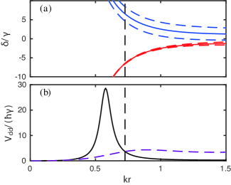
Figure 3: The sensitivity of DD interactions to the distance between an atom and its nearest neighbor. Here two two-level atoms are positioned so that their axis of separation is perpendicular to the direction of propagation of the driving plane wave and the dipoles are perpendicular to the axis of separation. (a) The shift $\delta$ of the superradiant collective mode (blue, solid top curve) and subradiant mode (red, solid lower curve) of the two atoms as a function of the distance between them. The dashed lines that bracket the solid lines indicate the collective widths of the modes. (b) The DD interaction energy $V_{\rm dd}$ as a function of the separation distance. The two curves are for the driving light tuned to the resonance frequency of the superradiant mode of the atoms when separated by the mean distance between the atoms in a cloud of $N=450$ atoms as in Fig. 2 (solid line), and to the single-atom resonance (dashed line).

In the case of two atoms, there are two collective eigenmodes for the optical response, each with a distinct frequency and decay rate. The frequencies and decay rates are shown in Fig. 3(a). As a result of the DD interactions mediated by the electric field, the eigenfrequencies of the nonrelativistic theory diverge in the limit of vanishing distance between the atoms as $1/r^{3}$. In this same limit the linewidth of one of the modes approaches $2\gamma$, twice the linewidth of an individual atom, and the linewidth of the other mode tends to zero. We call these modes, respectively, superradiant and subradiant Dicke (1954); Gross and Haroche (1982).

Figure 3(b) shows the strength of the DD interaction

$$V_{\rm dd} = -{\cal D}\mathcal{P}^{(1)\ast}\hat{\mathbf{{e}}}_{y}\cdot\mathbf{E}_{S}^{(2)}(\mathbf{X}_{1})$$ (19)

$$-{\cal D}\mathcal{P}^{(2)\ast}\hat{\mathbf{{e}}}_{y}\cdot\mathbf{E}_{S}^{(1)}(\mathbf{X}_{2})+{\rm c.c.}$$

as a function of the distance between the two atoms for two different fixed tunings of the driving light. The interaction tends to zero at short distances.

Our example presents two important lessons about DD interactions between two atoms. First, as the characteristic frequencies of the collective modes $\delta_{n}$ diverge at short distance, the external drive will no longer excite the collective modes [c.f. Eq. (16)]; nor will the individual atoms be polarized. Moreover, even if the DD interaction formally seems to diverge as $1/r^{3}$ at short distances, the decoupling of the atoms from the driving light wins out. One might surmise that at very short distances the DD interaction between two atoms becomes a calamity. Not so: Both atoms drop out of consideration altogether. Second, when the characteristic distance between the atoms is comparable to $1/k$, their interactions with light depends sensitively on their relative positions. Local density fluctuations are important, and the conventional electrodynamics for a many-atom system that assumes that the density of the atoms is sufficient to characterize their interactions with light is liable to break down.

III.2 Coupled dynamics of ⁸⁷Rb atoms

The multilevel structure of alkali-metal atoms, such as ⁸⁷Rb complicates, the collective dynamics of a cold gas with respect to that of two-level gases Pellegrino et al. (2014); Jenkins et al. (2016). Rather than atoms beginning in a single ground state, they could in principle occupy any linear combination of Zeeman ground states before the incident field interacts with the ensemble. Furthermore, different polarizations of light interact with the various transitions between Zeeman states in the ground and hyperfine levels in different ways according to the corresponding Clebsch-Gordan coefficients. Here, we simulate the response of an atomic cloud whose atoms are in an incoherent mixture of Zeeman levels. We will then discuss the dynamics of an individual stochastic realization, and examine the distributions of collective resonance frequencies and decay rates that appear in a dense cloud of atoms.

III.2.1 Dealing with Zeeman states

In the experiments the optical pumping process prepares each atom in an incoherent mixture of Zeeman states $\left|g,M\right\rangle$ with probabilities $p_{M}$ ($\sum_{M}p_{M}=1$), where $M=-g,\ldots,g$ indicates the magnetic quantum number of a state in the hyperfine level $g$. To account for this incoherent mixture in our stochastic simulations, for each realization of atomic positions $\{\mathbf{X}_{1},\ldots,\mathbf{X}_{N}\}$ we also sample a magnetic quantum number $M_{j}$ from each atom $j$ according to the probability distribution $p_{M}$. In the discussion below the ground-state magnetic quantum numbers $M_{j}$ are constants characteristic of one particular realization of the $N$-atom sample.

The EM response of each atom is then characterized by three amplitudes $\mathcal{P}_{M_{j},M_{j}+\sigma}^{(j)}$, where $\sigma=-1,0,1$ is an index indicating the polarization, and $\mathcal{P}_{M_{j},\eta}^{(j)}$ is an amplitude corresponding to the $\left|g,M_{j}\right\rangle_{j}\leftrightarrow\left|e,\eta\right\rangle_{j}$ transition. In the low light-intensity limit, the electric dipole moment is

$$\mathbf{d}_{j}(t)={\cal D}\sum_{\sigma=-1}^{1}\mathcal{C}_{M_{j},\eta}^{(\sigma)}\hat{\mathbf{e}}_{\sigma}\mathcal{P}_{M_{j},\eta}^{(j)}(t)\,\textrm{,}$$ (20)

where $\mathcal{C}_{M,\eta}^{(\sigma)}\equiv\langle F_{e}\eta;1F_{g}|F_{g}M;1\sigma\rangle$ are Clebsch-Gordan coefficients for the corresponding dipole transition ($F_{f}$ is the total atomic angular momentum of hyperfine level $f$), and the polarization vectors are defined in Eq. (2). We use Greek indices to denote the Zeeman states of the excited level $e$, and adopt the convention that repeated Greek indices are summed over. Here we consider the case $F_{g}=2$ and $F_{e}=3$.

As with two-level atoms, each ⁸⁷Rb atom $j$ in our system is driven by the field $\mathbf{E}_{\rm ext}(\mathbf{X}_{j},t)$, which comprises the incident field $\boldsymbol{\mathbf{\cal E}}_{0}$ and the scattered fields $\mathbf{E}_{S}^{(l)}$ ($l\neq j$). As a result, the amplitudes of the atomic dipoles associated to a given transition have the dynamics

$$\frac{d}{dt}\mathcal{P}_{M_{j}\eta}^{(j)} = \left(i\Delta_{M_{j}\eta}-\gamma\right)\mathcal{P}_{M_{j}\eta}^{(j)}$$ (21)

$$+i\xi\sum_{l\neq j}\mathcal{C}_{M_{j},\eta}^{(\sigma)}\mathcal{G}_{\sigma\varsigma}^{(jl)}\mathcal{C}_{M_{l},\zeta}^{(\varsigma)}\mathcal{P}_{M_{l}\zeta}^{(l)}$$

$$+i\frac{\xi}{{\cal D}}\mathcal{C}_{M_{j},\eta}^{(\sigma)}\hat{\mathbf{e}}_{\sigma}^{*}\cdot\epsilon_{0}\boldsymbol{\mathbf{\cal E}}_{0}({\bf r},t)\text{,}$$

where the amplitudes are coupled through the DD interaction between dipoles of orientation $\hat{\mathbf{e}}_{\sigma}$ and $\hat{\mathbf{e}}_{\varsigma}$,

$$\mathcal{G}^{(jl)}_{\sigma\varsigma}=\hat{\mathbf{{e}}}^{\ast}_{\sigma}\cdot\mathsf{G}(\mathbf{X}_{j}-\mathbf{X}_{l})\hat{\mathbf{{e}}}_{\varsigma}.$$ (22)

In addition to the incident and scattered electric fields, the applied $B=1\,\mathrm{G}$ bias field in the $x$ direction shifts the individual Zeeman levels. The resonance frequency of the $\left|g,M\right\rangle\leftrightarrow\left|e,\eta\right\rangle$ transition is shifted so that the incident field is detuned from that transition by

$$\Delta_{M\eta}\equiv\omega-\big{[}\omega_{0}+\frac{\mu_{B}B}{\hbar}(g_{e}M-g_{g}\nu)\big{]}\,,$$ (23)

where the Landé g-factors are $g_{g}\approx 0.50$ and $g_{e}\approx 0.67$, and $\omega_{0}$ is the resonance frequency unperturbed by the magnetic bias field. The total electric field elsewhere except at the position of the atoms is

$$\mathbf{E}({\bf r},t)=\boldsymbol{\mathbf{\cal E}}_{0}({\bf r},t)+\frac{{\cal D}}{\epsilon_{0}}\sum_{j}\mathcal{C}_{M_{j},\eta}^{(\sigma)}\mathsf{G}({\bf r}-\mathbf{X}_{j})\hat{\mathbf{e}}_{\sigma}\mathcal{P}_{M_{j},\eta}^{(j)}(t)\,.$$ (24)

The steady-state response then follows from

$${\cal D}\mathcal{P}_{M_{j}\eta}^{(j)}=\alpha_{M_{j}\eta}\sum_{\sigma}\mathcal{C}_{M_{j},\eta}^{(\sigma)}\hat{\mathbf{e}}_{\sigma}^{*}\cdot\epsilon_{0}\mathbf{E}_{\rm ext}(\mathbf{X}_{j},t)\,,$$ (25)

where the polarizability now reads

$$\alpha_{M_{j}\eta}=-{{\cal D}^{2}\over\hbar\epsilon_{0}(\Delta_{M_{j}\eta}+i\gamma)}\,.$$ (26)

The construction of the collective modes and their use in the analysis of the response of the system proceeds in the same way as with the two-level system, except that the vector of polarization amplitudes $\mathrm{b}$ for $N$ atoms is now made of the $3N$ polarization amplitudes $\mathcal{P}_{M_{j}\eta}^{(j)}$ with $\eta=M_{j}-1,M_{j},M_{j}+1$. In our analysis of the Rb cloud we will also introduce an inhomogeneous broadening for the resonance frequencies similarly as it was explained in the case of two-level atoms.

The numerical results shown in this paper have been tested by two independently developed sets of codes. The codes are based on a collection of C++ classes capable of handling an arbitrary angular momentum degenerate multilevel atom dipole-coupled to an arbitrary set of driving fields, etc. The same numerical methods have also been applied to solving collective electromagnetic response of plasmonic and microwave resonator arrays Jenkins and Ruostekoski (2012a); Adamo et al. (2012); Jenkins and Ruostekoski (2013), with appropriate extensions to include the magnetic properties of these materials.

IV Numerical and experimental results

In this section we present numerical simulation results and experimental findings of the optical response of an atomic ensemble in an elongated, ellipsoidal trap. The experimental setup is explained in Sec. II and concerns a cold ⁸⁷Rb vapor with several internal electronic ground states participating in the light scattering processes. In numerical simulations we also compare the cold-atom simulations with those of a thermal vapor. We begin by analyzing some generic collective properties of the atomic ensemble by calculating the collective radiative excitations modes of the atoms and the corresponding collective radiative resonance linewidths and line shifts.

IV.1 Cooperative modes

The collective mode characteristics for a particular realization of atomic positions strongly influence the response of the ensemble as a whole. As seen in Eqs. (14) and (15), the closer the collective resonance frequencies and decay rates are to those of a single atom, the better the scattering dynamics can be approximated by independent atoms. A broad distribution of resonance frequencies or decay rates, as will be evidenced in Secs. IV.2 and IV.3, alters the optical response.

IV.1.1 Eigenmodes

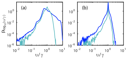
Figure 4: Distribution of collective mode decay rates in a cloud of homogeneously broadened (cold) ⁸⁷Rb atoms (a), and in an inhomogeneously broadened (hot) cloud in which the single-atom resonance frequencies have a Gaussian distribution with the root-mean-square width $\Omega=100\gamma$ (b). The samples contain $N=50$ (light bottom curve) and $N=450$ (dark top curve) atoms. The distributions were computed from a histogram of the values of $\log_{10}(\upsilon_{n})$ generated by $51200$ samples of atomic positions in which the Zeeman states have initial populations $p_{0}=p_{1}=p_{2}=1/3$ and $p_{-1}=p_{-2}=0$.

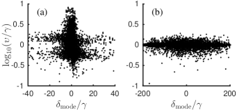
Figure 5: Representation in the complex plane of the eigenvalues associated with the collective modes for a particular realization of the atomic positions. Each mode is represented by a point, with the coordinates being the mode resonance frequencies $\delta_{n}$ and its decay rates $\gamma_{n}$. (a) Homogeneously and (b) inhomogeneously broadened (with a root-mean-square Gaussian width of $100\gamma$) samples of 450 ⁸⁷Rb atoms.

Figure 4 shows the distribution of the logarithm of collective mode decay rates $\log_{10}(\upsilon/\gamma)$ for cold (homogeneously broadened) and thermal (inhomogeneously broadened) gases of ⁸⁷Rb atoms with $N=450$. This distribution represents the probability density of obtaining a particular value of $\log_{10}(\upsilon/\gamma)$ on randomly selecting a collective mode from a gas with randomly chosen atomic positions. We computed the distribution numerically from $51200$ realizations of atomic positions.

In a cold gas the number of atoms in the ensemble strongly influences the width of the distribution of the collective decay rates. The system may support collective modes with subradiant and superradiant decay rates spanning several orders of magnitude. For $N=50$ and $N=450$ cold ⁸⁷Rb atoms, one percent of collective modes have decay rates of less than $0.45\gamma$ and $0.39\gamma$, respectively, and the median linewidths in these samples are $0.98\gamma$ and $0.79\gamma$, respectively. The inhibition of the light-mediated interactions in thermal ensembles is also shown in the distribution of the decay rates that is notably narrower. For both $N=50$ and $N=450$ atoms, the median linewidth matches that of a single atom, while one percent of the collective decay rates are below $0.90\gamma$ and $0.62\gamma$, respectively. Overall, we find that increasing the density of cold atoms makes the median value of the linewidth smaller, and generates a long tail of subradiant mode decay rates.

One can also see how collective modes differ in cold and thermal gases by examining the joint distributions of $\delta_{n}$ and $\log_{10}\upsilon_{n}$. Scatter plots of $\delta_{n}$ and $\log_{10}\upsilon_{n}$ obtained from five realization of atomic positions in samples of 450 atoms are shown in Fig. 5. In a cold gas, many of the mode resonance frequencies are shifted from the single-atom resonance, while collective decay rates span several orders of magnitude. The eigenmodes that exhibit larger resonance shifts also tend to be either fairly subradiant or superradiant and do not have linewidths that are close to the linewidth of a single isolated atom, indicating that large resonance shifts are correlated with the changes in the decay rates. Interestingly, the largest shifts are not associated with the most subradiant or superradiant modes.

The distribution of mode resonance frequencies in the inhomogeneously broadened sample, on the other hand, mostly reflects the Gaussian distributions of single-atom resonance frequencies. Furthermore, the collective mode decay rates closely match single-atom decay rates, indicating that the atoms respond to light nearly independently.

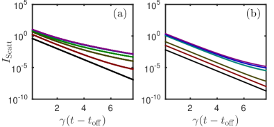
Figure 6: The simulated scattered power collected by the lens as a function of time after a $125$ns square excitation pulse is turned off for (a) a homogeneously broadened sample, and (b) an inhomogeneously broadened sample of ⁸⁷Rb atoms with the Doppler broadening of $100\gamma$. Here the atoms are trapped in a thermal equilibrium during and after the pulse. We show the intensity scattered into the detection apparatus (the curves from bottom to top) for the atom numbers $N=1$ (black), $N=5$ (red), $N=20$ (brown), $N=50$ (green), $N=200$ (cyan), $N=325$ (blue), and $N=450$ (purple). The light is on single-atom resonance. The varying rates of decay in the homogeneously broadened sample indicate the participation of both superradiant and subradiant collective modes, while the constant decay rates of the inhomogeneously broadened samples at the lowest atom numbers indicate that the atoms are radiating independently.

IV.1.2 The decay of collective modes

The role different collective decay rates play in the optical response of the ensemble can be inferred by calculating the temporal profile of scattered light. Consider a $125$ns square pulse, tuned to the frequency that, on average, most strongly scatters from a single ⁸⁷Rb atom. Here, for simplicity, we neglect the rise and fall times. After the pulse is turned off, the collective modes with higher decay rates contribute most strongly to light emission. But later, when more subradiant modes are present in the ensemble, the reduction in scattered light intensity slows with time, reflecting the excitation of subradiant modes that live longer. This behavior is illustrated for samples of various numbers of atoms in Fig. 6. Samples with more atoms, and hence broader distribution of decay rates, produce scattered radiation with a temporal profile that decays more slowly as time goes on. The deviations of the curves from straight lines in Fig. 6 indicate the co-existence of different exponential decay rates in the temporal profile. These represent non-negligible atom populations of different collective modes that exhibit different linewidths. In a thermal gas, where inhomogeneous broadening weakens DD interactions, this effect of subradiant modes requires higher densities to manifest itself than in a cold gas.

Using a cold and low-density, but optically thick, atom vapor the effects of subradiance were recently observed Guerin et al. (2016a). In these experiments the long tails of the decay distribution indicated the existence of subradiant mode excitations. Our simulations show that the signal in a dense gas could be notably enhanced.

IV.2 Experimental measurements of scattered light

The experimental setup was described in Sec. II. Reference Pellegrino et al. (2014) reported measurements of light scattering performed by sending a series of light pulses on the atomic cloud, hereafter referred to as the “burst excitation” method. Additional experimental protocols based on imaging with a single laser pulse were reported in Ref. Jenkins et al. (2016). These were used to rule out potential systematics and check the robustness of the resonance shift measurements of Ref. Pellegrino et al. (2014).

IV.2.1 Burst excitation method

In the first experiments described in detail in Ref. Pellegrino et al. (2014), we excited the cloud with 125 ns long pulses with flat-top temporal profile (rise time 7 ns) while the cloud had been released in free flight for 500 ns. The switching-off of the dipole trap was meant to eliminate light shifts caused by the trapping laser. The atomic density was nearly frozen during this period. However, as the amount of scattered light collected in a single realization of the experiment was very small, corresponding to less than $10^{-3}$ photons, we recycled the cloud many times and repeated sequences of excitation and recapture two hundred times with the same cloud of atoms. Excitation pulses were thus interleaved with $1\,\mathrm{\mu s}$ periods of recapture in the dipole trap. Further runs were then performed with newly prepared atomic clouds. The duration of the excitation pulse of $T=2.4/\gamma=125$ ns results from a compromise: it allows the atoms to approach the steady state, while minimizing the heating of the atoms. The choice of the number of sequences of excitation and recapture is then a trade-off between getting a good signal-to-noise ratio and avoiding light assisted losses Fuhrmanek et al. (2012) or heating of the cloud, as both effects would lower the cloud’s density. We have checked that the temperature of the cloud did not rise by more than $5\%$ after the entire set of pulses and that less than $5\%$ of the atoms were depumped in the $(5S_{1/2},F=1)$ hyperfine level.

For each excitation pulse, we recorded the total time-integrated power of the light scattered by the cloud arriving at the CCD camera, as shown in Fig. 1. For each number of atoms, we monitored the amount of scattered light as a function of the detuning of the excitation laser. As shown in Ref. Pellegrino et al. (2014), the lines are well fit by a Lorentzian. From the fit we extracted the amplitude $A$, the shift of the center of the line $\delta\omega_{\rm c}$, as well as the HWHM $\gamma_{\rm c}$. The results for the shift and the width are plotted in Figs. 7 and 8 as a function of the peak atomic density $\rho$ of the cloud. The latter is calculated from the measurement of the number of atoms, the temperature, and the knowledge of the trapping potential. Each point, for a given atom number, corresponds to an average over typically $1000$ newly-loaded clouds. We observe a small red-shift ($|\delta\omega_{\rm c}|\lesssim 0.3\gamma)$ and a broadening of the line, showing a sharp increase with the density for $\rho\lesssim 10^{14}$ at/$\rm cm^{3}$.

Let us consider now an incident field tuned to the frequency that maximizes the scattered intensity from a single atom. If $N$ atoms were to scatter independently, the fluorescence of the ensemble would be $N$ times that of a single atom. We find that the light scattered in the $z$ direction at resonance does not increase linearly with the number of atoms as one would expect for noninteracting atoms, but actually increases more slowly. It is shown in Fig. 9 that this is also the case off resonance. We observe that the amount of scattered light is strongly suppressed on resonance as the number of atoms increases, and that we gradually recover the behavior of noninteracting atoms as we detune the laser away from resonance.

IV.2.2 Complementary protocols

To rule out possible systematics due to the repetition of excitation pulses, we performed complementary measurements using the protocol described above Jenkins et al. (2016) but where we reduced the number of pulses per burst . The results, which we report in Figs. 7 and 8, do not indicate any significant change. While this does not entirely exclude the possibility of variations of the density during a single pulse, it does rule out the possible cumulative effect from sending several pulses on the same cloud. Finally, we performed measurements with excitation intensities at even lower levels (down to $I/I_{\rm sat}=0.001$). We still did not see any significant shift in the resonance.

In order to check for the robustness of the absence of the shift in a cold atomic sample, we also implemented a new protocol for the excitation. Instead of varying the density by modifying the atom number we change the geometry of the cloud. After having trapped $\sim 450$ atoms, we switched off the trap and varied the free-flight period $\Delta t$ during which the density of the atoms drops as $N/[(2\pi)^{3/2}\sigma_{x}\sigma_{y}\sigma_{z}]$, with $\sigma_{i}^{2}(\Delta t)=\sigma_{i}^{2}(0)+k_{B}T(\Delta t)^{2}/m$ ($i=x,y,z$), and the aspect ratio of the cloud evolves from a highly elongated cigar-shaped cloud to a spherical cloud. We then imaged the atoms with a $2\,\mu$s pulse at a given detuning and repeated the experiment $\sim 1000$ times using a new cloud each time. The results for the resonance shifts and widths are shown in Figs. 7 and 8 as a function of the peak density of the cloud at the beginning of the excitation pulse . The density is again deduced from the independent measurements of the trap size, atom number, and temperature of the cloud. Importantly, the various experimental protocols were implemented over a period of several months and with numerous adjustments to the experimental apparatus, but the results consistently indicate a very small resonance shift, and a broadening of the line with the same general shape.

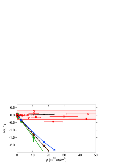
Figure 7: Line shift as a function of the atom density. Filled red circles: excitation with bursts of $200$ light pulses; each point corresponds to a different number of atoms. Upper and lower red triangles: excitation with respectively 75 and 1 pulses per burst. Empty red circles: excitation with one pulse after a variable time of flight; the cloud contains $\sim 450$ atoms. The shaded area indicates the laser linewidth of $\pm 0.3\gamma$. The error bars on the densities result from the cumulated measurement uncertainties on the trap size ($\sim 10\%$), atom number ($\sim 10\%$) and temperature ($\sim 10\%$). Decreasing values of the density correspond to time-of-flights $\Delta t=(0.7,1.7,2.7,3.7,4.7,6.7,8.7,20.7)\mu$s. Error bars on the experimental shift are from the fit of the fluorescence resonance spectrum by a Lorentz function. Numerical simulations: Shift of the line for homogeneously (black empty squares) and inhomogeneously broadened samples with root-mean-square spectral broadening of $10\gamma$ (blue crosses), $20\gamma$ (brown diamonds), and $100\gamma$ (green circles). Error bars: $95\%$ confidence intervals on the shift obtained from the fit of the spectrum to the Voigt profile (see text). Dashed line: estimated Lorentz-Lorenz shift.

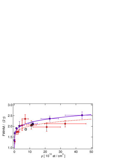
Figure 8: Full width at half maximum of the lines from the experiments where many bursts are sent onto the cloud (purple squares), and from probing the cloud after a time-of-flight measurement (red circles). Also shown are the results of the burst experiment for different number of pulses sent onto the cloud. The open square correspond to 350 atoms, at 190 $\mu$K, probed with a single pulse. Open circle: 350 atoms at 140 $\mu$K, one pulse. Open triangle: 340 atoms at 150 $\mu$K, 75 pulses. Error bars on the densities: same as in Fig. 7. Error bars on the width are from the fit of the fluorescence spectrum to a Lorentz function. The solid and dashed lines are phenomenological fits by a power law to the burst and time-of-flight method data, respectively.

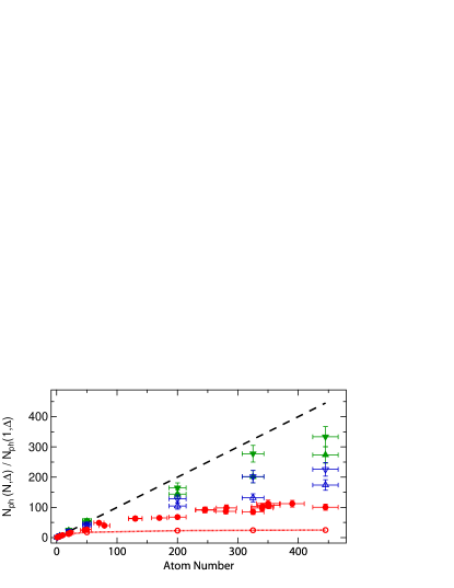
Figure 9: Amount of scattered photons $N_{\rm ph}(N,\Delta)$ detected in the $z$ direction, versus the number of atoms $N$, for different detunings $\Delta$ of the laser. The number of detected photons for each atom number is normalized to the single atom case, $N_{\rm ph}(1,\Delta)$, at the same detuning. The detunings are $\Delta=0$ (red circle), $\Delta=\pm 2\gamma$ (up/down open triangles), and $\Delta=\pm 5\gamma$ (up/down filled triangles). Red line: result of the numerical simulation of a homogeneously-broadened gas.

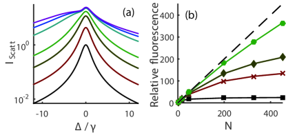
Figure 10: (a) Scattered intensity from an ensemble of ⁸⁷Rb atoms as a function of detuning $\Delta$. Light is scattered from an ensemble (the curves from bottom to top) with $N=1$ (black), $N=5$ (red), $N=20$ (brown), $N=50$ (green), $N=200$ (cyan), $N=325$, and $N=450$ (purple) atoms. (b) relative fluorescence as a function of number of atoms for homogeneously (black squares) and inhomogeneously broadened samples with root-mean-square spectral broadening of $10\gamma$ (red crosses), $20\gamma$ (brown diamonds), and $100\gamma$ (green circles). The dashed line denotes the result for noninteracting atoms.

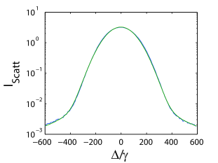
Figure 11: The light scattered from an inhomogeneously broadened ($100\gamma$) sample of 450 atoms in the presence of a $1G$ magnetic field as a function of driving frequency. The scattered intensity calculated from numerical simulations and the fit to the Voigt profile are virtually indistinguishable.

IV.3 Simulations of the optical response

The basic procedures of the numerical simulations of the multilevel ⁸⁷Rb experiment are described in Sec. III.2 where we model the experimental setup described in Sec. II. The inhomogeneous broadening is introduced using the techniques explained in Sec. III.1.2. From the response of the atomic dipoles to the incident field, we then calculate the intensity scattered into the detection apparatus as in the experimental configuration: the lens with numerical aperture $0.5$ gathers light in the far field centered on the $-z$ direction, and the signal passes through a polarizer rotated about $-\hat{\mathbf{{e}}}_{z}$ by $55^{\circ}$ from the $x$ axis.

IV.3.1 Fluorescence spectrum

Figure 10 shows the integrated scattered intensity as a function of $\Delta=\omega-\omega_{0}^{\prime}$ for numbers of atoms $N=1$-$450$, where $\omega_{0}^{\prime}$ is the frequency at which a single ⁸⁷Rb atom scatters the most incident light in the presence of the magnetic field. Calculations on few-atom cold ensembles produce the expected Lorentzian line shapes for the spectra of the scattered intensity. As $N$ increases, the spectral response begins to deviate from the independent atom scattering both in width and in the power of scattered light Pellegrino et al. (2014). The spectral response in the numerics becomes both broader and more asymmetric, with a fat tail that drops off more slowly for red-detuned incident fields than for blue detuning. As the numerically calculated spectrum cannot be modeled by a Lorentzian, extracting the value of the width is difficult. More quantitative comparisons between the theory and the measurements may be obtained from (1) the shift of the resonance and (2) the suppression of the computed peak fluorescence per atom relative to that of a single atom.

IV.3.2 Resonance shifts

Figure 7 shows the experimental shifts, which are deduced from Lorentzian fits to the measured spectra, together with the shifts deduced from the coupled-dipole simulations by simply taking the detunings corresponding to the maxima of the fluorescence intensity. Both shifts are negligible over the range of densities explored here, and are generally smaller than the linewidth of the laser $\sim\gamma/3$ in the experiments.

By contrast, in the simulations we may also introduce the Doppler broadening associated with the thermal Maxwell-Boltzmann distribution of the atomic velocities, and find the resonance shift by fitting to a Voigt lineshape. We find notably larger shifts Jenkins et al. (2016). For the Doppler width of $10\gamma$, corresponding to the temperature of $5.5$ K, the shift is, e.g., at the density $\rho=2.4\times 10^{14}$ cm^-3, already $50$ times larger than the stationary-atom result. Increasing the Doppler broadening further has a weaker effect on the shift. The quality of the fit of the Doppler-broadened lineshape to the Voigt profile is illustrated in Fig. 11.

In continuous effective-medium electrodynamics a natural energy scale for the resonance shifts is the Lorentz-Lorenz (LL) shift $\Delta_{\rm LL}=-2\pi\gamma\rho/k^{3}$, and at low atom densities $\rho$ one expects a shift of a resonance $\propto\rho/k^{3}$ also from dimensional analysis. We may estimate the LL shift by $\rho$ at the center of the trap (dashed line in Fig. 7). We find that the LL shift is absent both in the experiments and in the electrodynamics simulations of a cold gas. By contrast, introducing inhomogeneous broadening restores a resonance shift that is roughly equal to the LL shift $\Delta_{\rm LL}$, as illustrated in Fig. 7.

The difference between the optical responses of the cold and thermal atomic ensembles may be understood by the change in the light-induced DD interactions. With increasing inhomogeneous broadening the atoms are simply farther away from resonance with the light sent by the other atoms, which reduces the light-mediated interactions Javanainen et al. (2014). Moreover, the response of a cold, dense vapor is characterized by the many-atom collective excitation modes. In our case (this generally depends on the geometry of the sample and the excitation protocol ) the highly excited modes exhibit resonance frequencies close to the single atom resonance, and the shift in the observed spectrum consequently is small. In contrast, in thermal ensembles the shift can be qualitatively attributed to the standard local-field corrections Jackson (1999); Born and Wolf (1999) that give rise to the LL shift.

IV.3.3 Scattered intensity

In addition to the absence of the resonance shift, the collective response suppresses the resonant fluorescence. The numerical calculations predict the suppression of the scattered light when the number of atoms increases Fuhrmanek et al. (2012); Pellegrino et al. (2014). The homogeneously broadened case, as shown in Fig. 9, is in good agreement with the experimental data for $N\lesssim 50$. For $N\gtrsim 50$, the agreement is only qualitative, as the effects of the dipole-dipole interactions are found to be less pronounced experimentally.

By contrast, as shown in Fig. 10(b), adding a small amount of inhomogeneous broadening reduces the suppression of the scattering. The fluorescence of the inhomogeneously-broadened samples eventually also approaches the ideal limit of noninteracting atoms as the broadening reduces the interactions.

IV.3.4 Finite pulse duration

The results shown thus far indicate how the ensemble of atoms would scatter in the steady state when exposed to a monochromatic driving field of frequency $\omega$. In the experiments, on the other hand, the atoms are excited by a pulse with a carrier frequency $\omega$ that is about $125$ ns long. The apparatus then captures the scattered intensity integrated over time for each pulse. The spectral width of the driving pulse would tend to smoothen out some of the features that appear in the steady-state responses, since the time integrated response is proportional to a convolution of the pulse spectrum with the steady-state spectral response.

Figure 12 compares the response of ensembles of ⁸⁷Rb atoms to two pulse profiles and to the steady-state illumination. One pulse is a square pulse with the temporal profile

$$\mathbf{E}_{\mathrm{sq}}(t)=E_{0}\hat{\mathbf{{e}}}_{\mathrm{in}}\Theta(t)\Theta(T-t)\,\textrm{,}$$ (27)

where $T$ is $125$ ns. The second is a smoothed square pulse that closely resembles the experimental pulse profile,

$$\mathbf{E}_{\mathrm{sm}}(t)=E_{0}\sqrt{\frac{1}{1+\exp\left(-\frac{t-t_{\mathrm{on}}}{\Delta{}t}\right)}-\frac{1}{1+\exp\left(-\frac{t-T-t_{\mathrm{on}}}{\Delta{}t}\right)}}\,\textrm{;}$$ (28)

here $T\simeq 124$ns and $\Delta t\simeq 7.56$ns is the pulse rise/fall time.

The scattered intensities shown in Fig. 12 are normalized to the peak single-atom integrated intensity for the respective pulse shape. Since the smoothed pulse is spectrally narrower than the square pulse, the resonance width is consistently slightly narrower than that of the square pulse. Both pulsed excitations, however, are broader than the steady-state response. The relative fluorescence of the smoothed pulse is also slightly smaller than that of the square pulse, but not suppressed as much as that of the steady state.

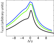
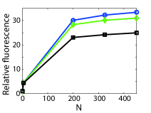
Figure 12: Differences between the responses to the steady-state and pulsed laser excitations. Left: The time integrated intensity scattered from $N=450$ atoms. Each curve is normalized to the peak time-integrated intensities scattered from a single atom driven by the incident field corresponding to that curve. Right: The peak relative fluorescence (at the frequency that maximizes scattering from a single atom) of the time integrated intensity as it depends on the number of atoms. Curves from bottom to top: the steady-state response (black), a smoothed square pulse [Eq. (28)] (green), and a square [Eq. (27)] (blue).

IV.3.5 Ground-state populations and Zeeman splitting

In the simulations discussed until now the populations of the initial state of the Rb atoms were always $p_{0}=p_{1}=p_{2}=1/3$. Our next topic about the simulations is the question about the sensitivity of the results to the initial state of the atom.

Figure 13 shows both the fluorescence line shape for a fixed large ($N=450$) number of atoms and the fluorescence intensity on resonance for a variable number of atoms for three different initial level populations of Rb, and indeed for the hypothetical two-level atom. The left-hand side panel shows that the level structure has a significant quantitative effect on the fluorescence intensity, but not on the line shift that was the object of our comparisons with the experiments. In the right-hand side panel the fluorescence intensities for different atom numbers are normalized to the maximum fluorescence intensity for a single atom with the same level structure and initial state. There is an effect from the level structure, but, when viewed in this way, it is not particularly dramatic.

In addition, we have tested the robustness of the simulation results to various other parameters in the experiments and have found no notable changes in the resonance shifts. For example, the Zeeman splitting due to the 1G magnetic field in the simulations does not significantly modify the response as compared with the zero field case. In a dense ensemble of ⁸⁷Rb atoms the main effect is to provide a slightly narrower resonance peak with a more recognizable ‘hump’ on the red-detuned side of the peak than in the absence of the magnetic field.

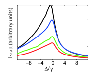
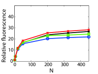
Figure 13: Left: The effects of Zeeman state populations on scattered intensity for an ensemble of $N=450$ ⁸⁷Rb atoms. The curves from top to bottom: the scattered intensity from two-level atoms (black), from ⁸⁷Rb with $p_{2}=1$ (blue), $p_{2}=p_{1}=p_{0}=1/3$ (green), and $p_{j}=1/5$ for all $j$ (red). Right: Relative fluorescence as a function of number of atoms, for an incident field tuned to a single atom’s peak fluorescence. The scattered intensity from an ensemble of atoms is normalized to the maximum of the scattered intensity from a single atom. The curves from top to bottom: the scattered intensity from ⁸⁷Rb with $p_{j}=1/5$ for all $j$ (red), two-level atoms (black), ⁸⁷Rb with $p_{2}=p_{1}=p_{0}=1/3$ (green), and $p_{2}=1$ (blue). The magnetic field is equal to zero.

V Concluding remarks

It has previously been shown in the case of coherent light transmission that in dense, homogeneously-broadened atomic ensembles strong light-mediated interactions and the resulting light-induced correlations can lead to a dramatic and qualitative failure of standard continuous effective-medium electrodynamics Javanainen et al. (2014); Javanainen and Ruostekoski (2016). This is because the standard textbook theory of optics Jackson (1999); Born and Wolf (1999) represents an effective-medium mean-field theory that assumes each atom interacting with the average behavior of the surrounding atoms. In such models the spatial information about the precise locations of the pointlike atoms – and the corresponding details of the position-dependent DD interactions – is washed out, resulting in the absence of the light-induced correlations.

In the presence of inhomogeneous broadening the results of the standard electrodynamics of continuous polarizable medium, however, can be restored Javanainen et al. (2014). At sufficiently high temperatures, the simulations qualitatively agree with the standard established models of resonance line shifts, the LL shift and its similarly mean-field theoretical collective (finite-size) counterpart, the “cooperative Lamb shift” Friedberg et al. (1973). The microscopic mechanism for the emergence of the continuous medium electrodynamics is the suppression of the light-mediated resonant DD interactions between the atoms: With increasing inhomogeneous broadening the atoms are simply farther away from resonance with the light scattered by the other atoms. Formally, one can show Javanainen et al. (2014) that in thermal ensembles each recurrent scattering event is suppressed by the factor $\sim\gamma/\Omega$, where $\Omega$ denotes the width of the inhomogeneous broadening.

Here we have explained in detail and extended our work of Refs. Pellegrino et al. (2014); Jenkins et al. (2016) on near-resonance light scattering from small clouds of cold or thermal atoms. We illustrated a substantially different behavior of resonance fluorescence of trapped, cold Rb atoms from that of thermal atoms. In our analysis we performed side-by-side comparisons between experimental observations and large-scale numerical simulations of resonance fluorescence in a dense cloud of ⁸⁷Rb atoms. Both the experiment and stochastic simulations demonstrate the emergence of collective DD interactions that dramatically alter the optical response as the number of atoms is gradually increased. We found that both the cold-atom simulations and the experimental observations of the resonance line shifts and the total collected scattered light intensity substantially deviate from those of thermal atomic ensembles. In particular, a density-dependent resonance shift of a thermal atomic ensemble is almost entirely absent in a cold atomic cloud. Our numerical models of fluorescence are also more involved than those of light transmission in Ref. Javanainen et al. (2014), and incorporate the experimental setup in detail, including the inhomogeneous atom densities due to the trapping potential, the internal multilevel structure of ⁸⁷Rb, and the imaging geometry with the optical components (e.g., lenses and polarizers).

Moreover, we analyzed the effect of strong light-mediated interactions between the atoms by calculating the collective radiative excitation eigenmodes of the system. As a result of light-induced DD interactions, the response of the sample becomes collective, exhibiting collective radiative resonance linewidths and line shifts including those with subradiant and superradiant character. When the collective radiative decay rates are far from those of a single isolated atom, the optical response of the cloud cannot be approximated by the one consisting of independent atoms, and a broad distribution of decay rates is an indication of strong DD interactions.

The role of collective excitation eigenmodes in the optical response is in particular illustrated by the calculation of the temporal profile of the decay of light-induced excitations after the incident laser pulse is switched off. At high atom densities the simulations predict a significantly slower decay for cold than for thermal atom clouds. In a logarithmic scale the calculated scattered power notably deviates from a straight line, indicating non-negligible occupations of (both superradiant and subradiant) collective modes with different radiative linewidths.