Identifying Phase Space Boundaries with Voronoi Tessellations

Abstract

Determining the masses of new physics particles appearing in decay chains is an important and longstanding problem in high energy phenomenology. Recently it has been shown that these mass measurements can be improved by utilizing the boundary of the allowed region in the fully differentiable phase space in its full dimensionality. Here we show that the practical challenge of identifying this boundary can be solved using techniques based on the geometric properties of the cells resulting from Voronoi tessellations of the relevant data. The robust detection of such phase space boundaries in the data could also be used to corroborate a new physics discovery based on a cut-and-count analysis.

1 Introduction

Voronoi tessellations Voronoi are useful in a wide variety of fields, from biology biology to astronomy Ramella:2001yt ; Cappellari:2003ir to condensed matter physics bowick . In high energy physics, they have been used rather sporadically, e.g., as an optional approach to QCD jet-finding and area determination in FastJet Cacciari:2011ma and in the model-independent definition of search regions in SLEUTH  Abbott:2000fb ; Abbott:2001ke ; Aaltonen:2007dg ; Aaltonen:2008vt . In Ref. Debnath:2015wra , some of us pointed out that Voronoi methods can be applied directly to the analysis of data from high energy physics experiments, e.g., when trying to detect the presence of a new physics signal in the data or to perform parameter measurements.

In most Voronoi-based approaches, the goal is to use Voronoi tessellations to identify “neighbors” of data points. The tessellation then automatically provides a number of cell-based attributes for each data point. Ref. Debnath:2015wra argued that using the geometric properties of Voronoi cells, and, in particular, functions of the geometric properties of Voronoi cells and their neighbors, gives valuable additional information and can allow for relatively model-independent searches for targeted “features” in the data. As briefly discussed in Ref. Debnath:2015wra , a particularly useful application is the study of kinematic edges when investigating cascade decays in new physics models such as supersymmetry (SUSY) Martin:1997ns .

To understand the importance of edge-finding in multidimensional spaces for SUSY mass measurement, we first note that many extensions of the standard model (SM) are characterized by a $\mathbb{Z}_{2}$ symmetry under which new physics particles (NPPs) are charged but the SM particles are uncharged. Such a symmetry ensures that the lightest NPP will be stable and hence may constitute the dark matter. With the assumption of such a symmetry, a typical collider event involving NPPs proceeds as follows:

1. NPPs are pair produced.

2. Each NPP goes through a series of (generally two and three-body) decays called a “decay chain”. In each decay, an NPP decays to another, lighter, NPP, and one or more SM particles. The NPPs generally have a small intrinsic width compared with their mass. Hence it is generally a good approximation to view the decay chain as consisting of a series of on-shell decays of NPPs.

3. Eventually the lightest particle charged under the $\mathbb{Z}_{2}$ is reached. It is stable, and, if a dark matter candidate, uncharged and uncolored. Hence it will escape the detector without being detected.

Popular new physics models within this paradigm include SUSY, where the $\mathbb{Z}_{2}$ symmetry is called “$R$-parity”; Universal Extra Dimensions (UED) Appelquist:2000nn , in which the $\mathbb{Z}_{2}$ symmetry is called “KK-parity”; and Little Higgs models, in which the $\mathbb{Z}_{2}$ symmetry is called “$T$-parity” Cheng:2003ju .

As the lightest NPP escapes detection, we are not able to determine directly the masses of the initial new physics particles produced in the collision, nor the masses of any intermediate particles in the decay, as we would if we were studying a resonance decaying to visible particles. However, we can determine the masses of the NPPs by studying the distributions of (functions of) the momenta of observed particles Barr:2010zj .

Much effort has gone into determining the best way to actually perform this mass measurement. The simplest methods involve finding an edge or an endpoint in the one-dimensional distribution of the invariant mass of two (or more) reconstructed objects  Hinchliffe:1996iu ; Bachacou:1999zb ; Allanach:2000kt ; Lester:2001zx ; Gjelsten:2004ki ; Gjelsten:2005aw ; Lester:2005je ; Miller:2005zp ; Lester:2006yw ; Ross:2007rm ; Barr:2008ba ; Barr:2008hv ; Cho:2012er . If one is able to measure enough of these kinematic endpoints, it is then possible to solve for the unknown masses, possibly up to discrete ambiguities  Gjelsten:2005sv ; Burns:2009zi ; Matchev:2009iw . This approach naturally evolved into the so-called “polynomial method”  Hinchliffe:1998ys ; Nojiri:2003tu ; Kawagoe:2004rz ; Cheng:2007xv ; Nojiri:2008ir ; Cheng:2008mg ; Cheng:2009fw ; Webber:2009vm ; Autermann:2009js ; Kang:2009sk ; Nojiri:2010dk ; Kang:2010hb ; Hubisz:2010ur ; Cheng:2010yy ; Gripaios:2011jm , where one attempts to solve explicitly for the momenta of the invisible particles in a given event, possibly using additional information from prior measurements of kinematic invariant mass endpoints. Since at hadron colliders the longitudinal momenta of the initial state partons are unknown, much effort went into the development of suitable “transverse variables” Lester:1999tx ; Barr:2003rg ; Baumgart:2006pa ; Lester:2007fq ; Tovey:2008ui ; Serna:2008zk ; Nojiri:2008vq ; Cho:2008tj ; Cheng:2008hk ; Burns:2008va ; Choi:2009hn ; Matchev:2009ad ; Polesello:2009rn ; Konar:2009wn ; Cho:2009ve ; Nojiri:2010mk , which are Lorentz-invariant under longitudinal boosts. In principle, the optimal approach to mass measurement is provided by the so-called “Matrix Element Method” (MEM), Kondo:1988yd ; Dalitz:1991wa ; Abazov:2004cs ; Alwall:2009sv ; Artoisenet:2010cn ; Alwall:2010cq ; Fiedler:2010sg ; Gainer:2013iya . However, its use is often computationally prohibitive, especially when dealing with complicated final states and/or large reducible backgrounds. Many of the approaches described above have been extended in various ways, e.g., the $M_{T2}$ kink method allows the measurement of the mass of the lightest NPP  Cho:2007qv ; Gripaios:2007is ; Barr:2007hy ; Cho:2007dh ; Nojiri:2008hy ; Barr:2009jv ; Matchev:2009fh ; Konar:2009qr , and useful $3+1$-dimensional analogues of the “transverse” invariant mass variables have been suggested Konar:2008ei ; Konar:2010ma ; Barr:2011xt ; Robens:2011zm ; Mahbubani:2012kx ; Bai:2013ema ; Cho:2014naa ; Cho:2014yma ; Cho:2015laa ; Konar:2015hea .

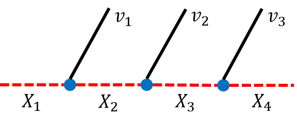
Figure 1: Decay process of a heavy resonance $X_{1}$ into three visible particles, $v_{1}$, $v_{2}$ and $v_{3}$, along with an invisible particle, $X_{4}$, via two on-shell intermediate states, $X_{2}$ and $X_{3}$. The NPPs, $X_{i}$, are denoted by red dashed lines while visible SM particles are denoted by black solid lines.

The approach to mass measurement taken here seeks to improve on those described in the existing literature in the following ways:

1. Instead of finding edges or endpoints in the one-dimensional distribution of a single variable, we will attempt to determine the boundary of the signal region in a higher-dimensional phase space. This improves on one-dimensional methods, in increasing greatly the amount of information that can be extracted from the data Agrawal:2013uka . To be specific, we shall consider the classic SUSY decay chain of three successive two-body decays as shown in Fig. 1. From the measured four-momenta, $p_{i}~{}(i=1,2,3)$, of the three visible particles, $v_{i}$, in the decay, one can form three two-body invariant mass combinations, $m_{ij}=\sqrt{(p_{i}+p_{j})^{2}}$, for $i<j$. Signal events will then populate the interior of a compact region, ${\cal V}_{3}$, in the three-dimensional phase space, $(m_{12},m_{23},m_{13})$, of invariant masses Costanzo:2009mq ; Kim:2015bnd . The size and the shape of the two-dimensional surface boundary of ${\cal V}_{3}$, which we term ${\cal S}_{2}$, contains the complete information about the underlying mass spectrum, $m_{X_{i}}(i=1,2,3,4),$ of the NPPs in Fig. 1. Therefore, we shall focus on methods for detecting ${\cal S}_{2}$ directly. One can imagine doing this in two ways:

   • By defining a kinematic variable which takes the same (constant) value (e.g., zero) everywhere along the phase space boundary. This approach will be discussed below in section 3, where we review the relevant variable, $\Delta_{4}$, introduced in Ref. Agrawal:2013uka .

   • By analyzing the measured density of events in phase space and locating the boundary, ${\cal S}_{2}$, directly using techniques inspired by spatial analyses performed in other fields of science. This will be the main subject of this paper, and will be discussed in sections 2.2, 3.2, 3.3, and 4.

2. We build on the idea of Ref. Debnath:2015wra that Voronoi tessellations provide a powerful and model-independent tool for identifying edges (for a brief introduction to Voronoi tessellations, see section 2.1 below). While the analysis of Ref. Debnath:2015wra was limited to data in two dimensions, here we extend the procedure to the three-dimensional case and try to delineate the region, ${\cal V}_{3}$, in the phase space of the three variables, $(m_{12},m_{23},m_{13})$. Before tackling a SUSY physics example in section 4, we consider several analogous toy examples of increasing complexity in sections 2 and 3. This helps develop the reader’s intuition and motivates some of our analysis choices. Following Ref. Debnath:2015wra , in order to select “edge” cells in the Voronoi tessellation of the data, we consider the relative standard deviation (RSD), $\bar{\sigma}_{i}$, of the volumes of neighboring cells, which is defined as follows. Let $N_{i}$ be the set of neighbors of the $i$-th Voronoi cell, with volumes, $\{v_{j}\}$, for $j\in N_{i}$. The RSD, $\bar{\sigma}_{i}$, is now defined by

   $$\bar{\sigma}_{i}\equiv\frac{1}{\langle{v}(N_{i})\rangle}\,\sqrt{\sum_{j\in N_{i}}\frac{\left(v_{j}-\langle{v}(N_{i})\rangle\right)^{2}}{|N_{i}|-1}},$$ (1)

   where we have normalized by the average volume of the set of neighbors, $N_{i}$, of the $i$-th cell

   $$\langle{v}(N_{i})\rangle\equiv\frac{1}{|N_{i}|}\sum_{j\in N_{i}}v_{j}.$$ (2)

   The variable defined in eq. (1) is a straightforward extension to three dimensions of the “scaled standard deviation” of neighbor areas found to be helpful in Ref. Debnath:2015wra .

3. We make crucial use of the recent observation of Ref. Agrawal:2013uka that for sufficiently many-body final states there is an enhancement (in fact a singularity) in the phase space density near the boundary, ${\cal S}_{2}$, of the allowed phase space, ${\cal V}_{3}$. Due to the enhancement in the density of signal events near the boundary of phase space, we can alternatively target the boundary points of ${\cal V}_{3}$ as being points in a densely populated region. This motivates us to consider, in addition to $\bar{\sigma}_{i}$, a second variable related to volume. We choose

   $$\bar{v}_{i}=\frac{v_{i}}{\langle{v}(N_{i})\rangle},$$ (3)

   where again we normalize by the average volume (2) of the set of neighbors, $N_{i}$.

In what follows, we will therefore focus on the two Voronoi-based dimensionless variables (1) and (3). The former is motivated by the discontinuity in the density of events at the boundary Debnath:2015wra , while the latter is motivated by the enhancement in the density of signal events at the boundary Agrawal:2013uka . We will find that the judicious combination of these two variables yields a significant increase in sensitivity as compared with either variable in isolation. As a result we find that we are able to identify the boundary, ${\cal S}_{2}$, of the allowed signal phase space, ${\cal V}_{3}$, with a high degree of accuracy, even when the ratio of signal to background events, $S/B$, is relatively small.

To support these conclusions, as well as to explain in detail to the reader the methods employed, we proceed as follows. In section 2 we will provide a brief, but sufficient, review of Voronoi tessellation methods and the use of the geometric properties of Voronoi cells for identifying features in high energy physics data. Section 3.1 will review the consideration of events in multi-dimensional phase space, and, especially the observation that, for sufficiently many dimensions, the differential phase space volume is highly peaked near the boundary. Then in sections 3.2 and 3.3 we study the efficacy of Voronoi methods for finding a densely populated spherical boundary in a generalized “phase space”, while section 4 will examine the application of these methods to an actual benchmark point. We present our conclusions in section 5. Throughout our studies, we will use ROC curves to quantify the sensitivity of the variables we define; we briefly review and discuss this approach in Appendix A.

2 Voronoi Methods for Finding Boundaries

Voronoi tessellation voronoi refers to the procedure, previously proposed by Dirichlet dirichlet and hinted at by Descartes descartes , through which an $n$-volume containing a set of $N_{d}$ data points, $\{d_{i}\}$, is divided into $N_{d}$ non-overlapping regions, $\{R_{i}\}$, such that $d_{i}\in R_{i},\forall i$. The boundaries of $R_{i}$ are chosen such that, for every point in some region $R_{j}$, the corresponding data point, $d_{j}$, is the nearest data point.

For applications in high energy physics, we consider the data points to be events in a suitably chosen phase space. It is important to make a judicious choice of phase space — on the one hand, it should be of low enough dimensionality to keep the problem tractable in practice, yet the dimensional reduction should not result in the loss of any useful information, e.g., the washing out of interesting features in the underlying phase space distributions. Consider, as an example, the decay chain of Fig. 1. In general, the inclusive production of the $X_{1}$ resonance will be described by a 9-dimensional phase space, consisting, e.g., of the nine momentum components of the visible particles, $v_{i}$. However, three of those degrees of freedom correspond to uninteresting Lorentz boosts of $X_{1}$, another three degrees of freedom are angular variables which are sensitive to spins but not the $X_{i}$ mass spectrum, leaving only the three degrees of freedom relevant to a mass measurement. As already mentioned in the introduction, we can take these three degrees of freedom to be the invariant mass quantities $(m_{12},m_{23},m_{13})$. We shall present the results from our analysis of this physics example in section 4, but we first begin with a few toy studies.

2.1 Voronoi tessellations in two dimensions

In order to make contact with Ref. Debnath:2015wra and to introduce our notation, we begin by studying several simplified scenarios in two dimensions. In the next section, (2.2), we will generalize the approaches taken and the lessons learned here to the case of three dimensions.

2.1.1 A linear boundary in two dimensions

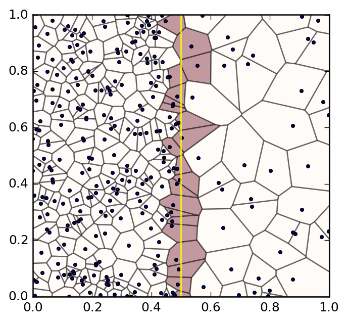
Figure 2: $N_{events}=280$ events distributed according to (4) with $\rho=6$ and the respective Voronoi tessellation. The shaded cells are those crossed by the boundary (vertical yellow line) and are defined to be the “edge cells”.

In Fig. 2, we consider the unit square in the first quadrant ($x\geq 0,y\geq 0$) and simulate $N_{events}=280$ events (data points) according to the probability distribution

$$f(x,y)=\frac{2}{1+\rho}\left[\rho H(0.5-x)+H(x-0.5)\right],$$ (4)

where $H(x)$ is the Heaviside step function and $\rho$ is a constant density ratio, taken in Fig. 2 to be $\rho=6$. The meaning of the distribution (4) is very simple: the unit square is divided into two equal halves by the vertical boundary at $x=0.5$ (the yellow line in Fig. 2). Within each half, the density is constant (on average), but the left region is denser by a factor of $\rho$. This setup produces an edge at $x=0.5$, where the density changes by a factor of $\rho$. Our goal will be to detect this edge by tagging the Voronoi cells that are crossed by the boundary line — such cells from now on will be referred to as “edge cells” and in Fig. 2 they are shaded in brown. The remaining Voronoi cells away from the edge will be referred to as “bulk” cells, and in Fig. 2 they are left white.

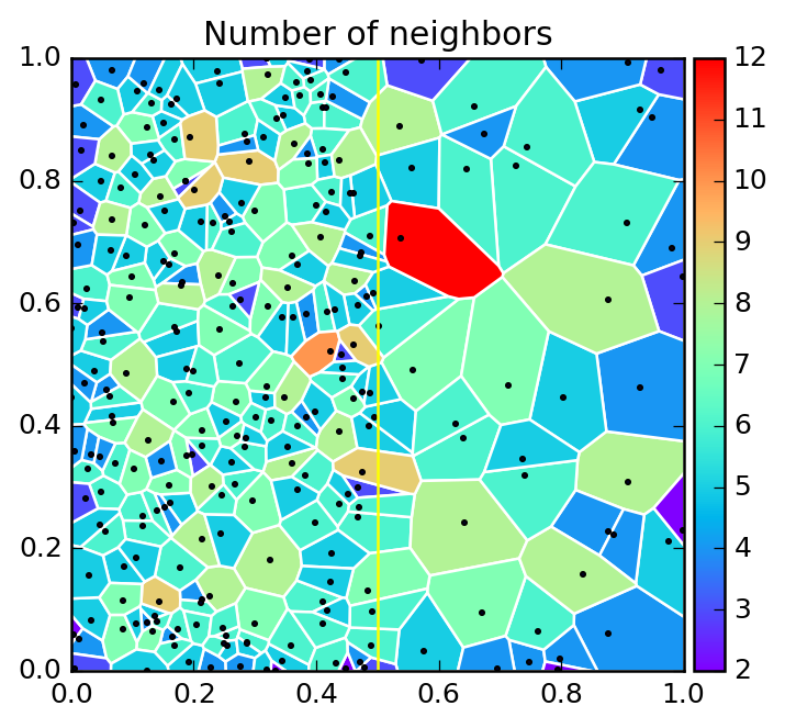
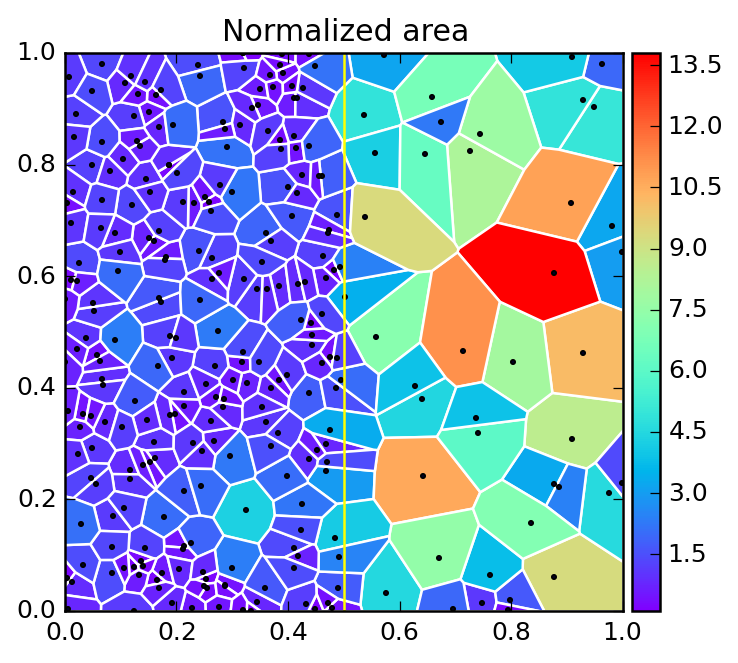
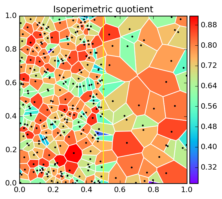
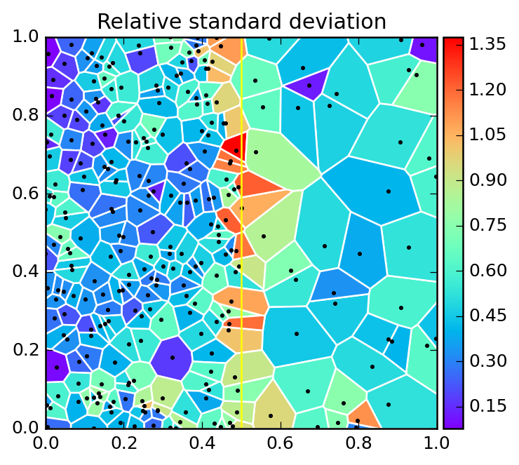
Figure 3: The Voronoi tessellation shown in Fig. 2, with cells color-coded according to the number of neighboring polygons (upper left), normalized area (7) (upper right), isoperimetric quotient (8) (lower left), and RSD (9) (lower right).

The basic idea put forth in Ref. Debnath:2015wra was to study the resulting Voronoi tessellation and identify edge cells from their geometric properties (as well as from the geometric properties of neighboring cells within the immediate vicinity). The Voronoi cells in two dimensions are planar polygons, for which one can investigate the usual geometric properties like number of sides, area, perimeter, etc. Fig. 3 shows four possibilities, where the Voronoi cells are color-coded according to the value of the corresponding geometric quantity. Then, in Fig. 4, we plot the probability distributions for these geometric quantities separately for the edge cells (red solid lines) and the bulk cells (blue dotted lines). As can be seen in Fig. 2, the edge cells, by construction, represent a very small fraction of the total number of Voronoi cells in the tessellation. Thus, in order to increase the statistical precision of the distributions in Fig. 4, we generated $N_{exp}=1000$ pseudo-experiments analogous to the one shown in Fig. 2.

In the upper left panels of Figs. 3 and 4, we study the number of elements, $|N_{i}|$, in the set of neighbors, $N_{i}$. This is equivalent to the number of sides of the $i$-th Voronoi polygon. This variable has been studied in the literature MilesMaillardet1982 : for example, it is known that the Voronoi polygons most commonly have 5 or 6 sides, which is confirmed in Figs. 3 and 4. There is also a long tail of polygons with many sides, which is conjectured to behave asymptotically as $|N_{i}|^{-2|N_{i}|}$ Drouffe:1983wr . Indeed, Fig. 2 contains an example of a polygon with as many as 12 sides! The upper left panel of Fig. 4 demonstrates that, as expected, the $|N_{i}|$ distributions for bulk and edge cells are rather similar, and are thus not suitable for tagging edge cells Debnath:2015wra .

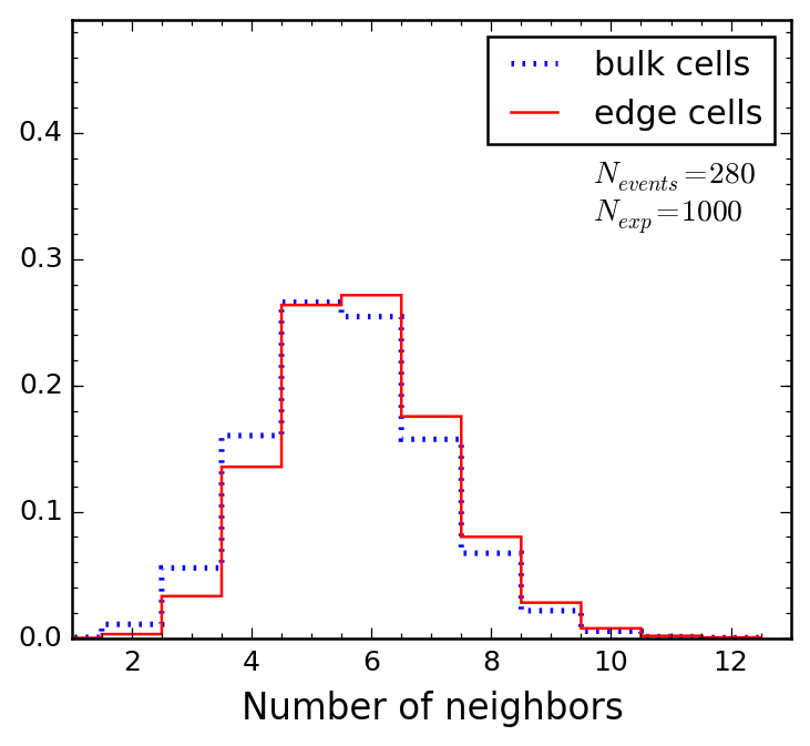
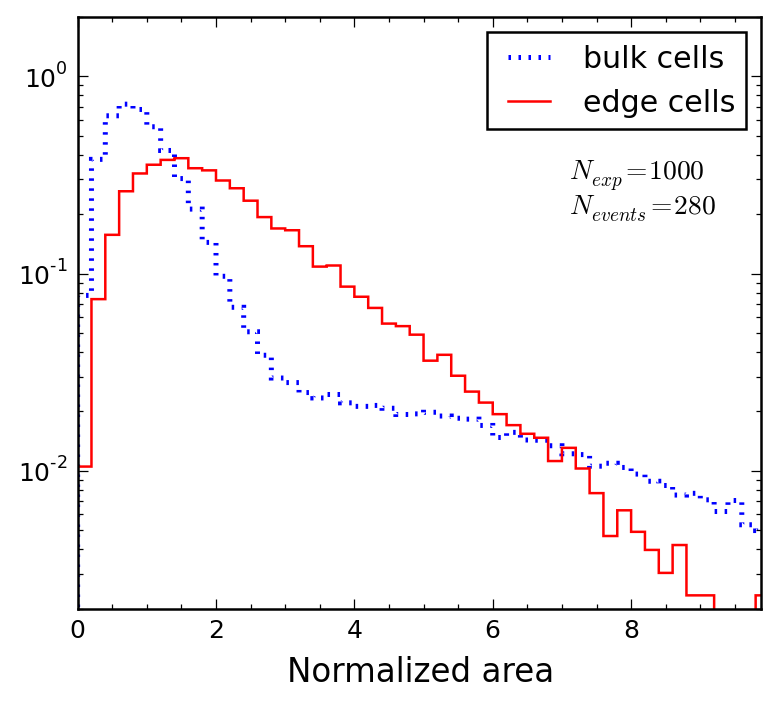
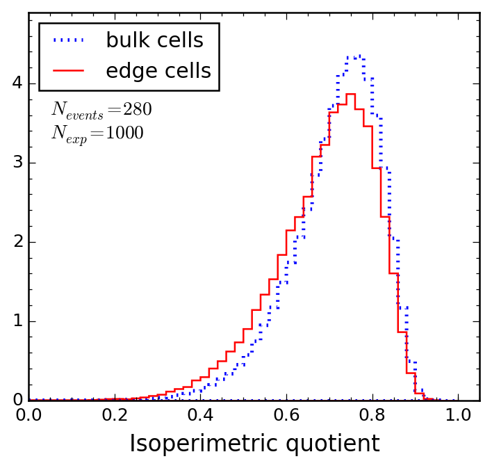
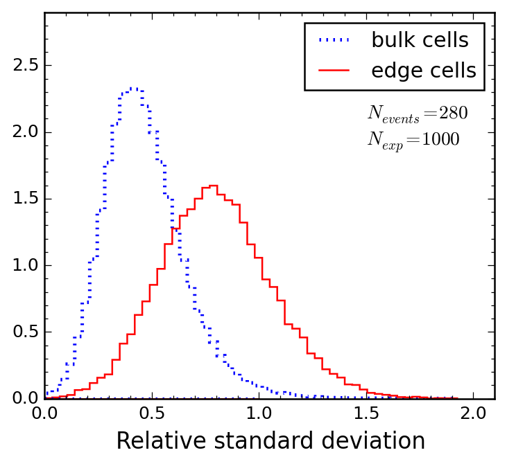
Figure 4: Unit-normalized distributions of the four Voronoi cell properties depicted in Fig. 3. Blue dotted (red solid) histograms refer to bulk (edge) cells. In order to increase the statistics, we show results from $N_{exp}=1000$ pseudo-experiments with $N_{events}=280$ each.

The upper right panels of Figs. 3 and 4 illustrate a different geometric quantity related to the areas, $a_{i}~{}(i=1,2,\ldots,N_{events})$, of the Voronoi cells. The areas of the Voronoi polygons are meaningful because they provide an estimate of the value of the underlying distribution $f(x,y)$ (4) at the corresponding data point $(x_{i},y_{i})$:

$$f(x_{i},y_{i})\approx\frac{1}{N_{events}\times a_{i}},$$ (5)

so that $f(x,y)$ is still unit-normalized:

$$\sum_{i=1}^{N_{events}}f(x_{i},y_{i})\times a_{i}=\frac{1}{N_{events}}\sum_{i=1}^{N_{events}}\frac{a_{i}}{a_{i}}=1.$$ (6)

In Figs. 3 and 4 we choose to normalize the cell areas not locally as in (3), but by the expected average area in the dense region. Thus, a typical bulk cell to the left of the vertical boundary has normalized area of approximately 1, while a typical bulk cell to the right of the boundary has a normalized area of approximately $\rho=6$. Note that while we fix the total number of events, $N_{events}$, the fraction which ends up on one side of the boundary varies — for example, in the single pseudo-experiment depicted in Figs. 2 and 3, there happen to be 243 events on the left side and 37 events on the right side (to be compared with the expectation of $\rho N_{events}/(\rho+1)=240$ events on the left side and $N_{events}/(\rho+1)=40$ events on the right side). If the total area is $A=\sum_{i}a_{i}$, the expected average size of a bulk cell in the dense region on the left is given by $A(\rho+1)/(2\rho N_{events})$, hence in the upper right panels of Figs. 3 and 4 we plot the cell areas, $a_{i}$, normalized as

$$\bar{a}_{i}=\frac{2\rho N_{events}}{\rho+1}\,\frac{a_{i}}{A}.$$ (7)

The distribution of the Voronoi cell areas when the points have been randomly selected (in a “Poisson process”) is not known analytically, and is typically approximated with a three-parameter generalized gamma function, where the parameters are fitted to results from Monte Carlo simulations HindeMiles1980 . For our purposes, we are not interested in the form of the actual distributions but in the question of whether the distributions for bulk and edge cells show any appreciable differences. As seen in the upper right panel of Fig. 4, the area distribution for bulk cells is nearly bimodal; with the normalization (7) two peaks are expected near $\bar{a}_{i}\sim 1$ and $\bar{a}_{i}\sim\rho=6$. The area distribution for edge cells, on the other hand, is unimodal, peaking relatively close to $\bar{a}_{i}\sim 1$. After all, we expect a larger fraction, namely $\rho/(\rho+1)$ of the edge cells, to have their centers on the “dense” side of the boundary and only $1/(\rho+1)$ of the edge cells to have their centers on the “sparse” side of the boundary. A close inspection of Fig. 2 confirms this expectation: out of the 21 edge cells, 18 (3) have their centers to the left (to the right) of the vertical boundary, which is consistent with our expectations for $\rho=6$. In conclusion, it is clear that in this case, the Voronoi cell area by itself is not a very good candidate for an edge-tagging variable Debnath:2015wra . We expect that in the more general situation, where the densities on each side of the boundary are not uniform, this variable will be even more unsuitable.

Having investigated a variable describing the size of the Voronoi polygon, we now examine a variable characterizing the shape of the polygon, e.g., the isoperimetric quotient

$$q_{i}\equiv\frac{4\pi a_{i}}{p_{i}^{2}},$$ (8)

where $a_{i}$ is the area and $p_{i}$ is the perimeter of the $i$-th Voronoi polygon. The variable (8) is a measure of “roundedness” — it is equal to zero for infinitely thin (pencil-like) polygons, and is equal to 1 in the limit of a perfectly symmetric polygon with infinitely many sides (i.e., a circle). The corresponding results for the isoperimetric quotient are shown in the lower left panels of Figs. 3 and 4. We observe that the edge cells tend to be slightly more “squashed”, but the difference is very minor and not useful in practice.

In a similar vein, one could continue to study other geometric characteristics of a single Voronoi cell, e.g., perimeter, average side length, etc. Debnath:2015hva , but, similarly, this is unlikely to lead to any success in identifying edge cells. The reason is that we are trying to detect a discontinuity and therefore we need to study the relative properties of cells on both sides of the boundary. One possibility is to compute a derivative quantity, e.g., the gradient at each cell location Debnath:2015wra . Another option is to compare the spread in the areas of the neighboring cells, e.g., by computing the RSD, $\bar{\sigma}_{i}$, of the areas of the cells in $N_{i}$ (the set of neighbors of the $i$-th Voronoi polygon) in analogy to (1) Debnath:2015wra :

$$\bar{\sigma}_{i}\equiv\frac{1}{\langle{a}(N_{i})\rangle}\,\sqrt{\sum_{j\in N_{i}}\frac{\left(a_{j}-\langle{a}(N_{i})\rangle\right)^{2}}{|N_{i}|-1}},$$ (9)

where the normalization now is done by the average area of the neighbors

$$\langle{a}(N_{i})\rangle\equiv\frac{1}{|N_{i}|}\sum_{j\in N_{i}}a_{j}.$$ (10)

The idea is very simple — the neighbors of edge cells are typically quite diverse — some happen to be on the dense side and are therefore relatively small, while others are on the sparse side and are relatively large. As a result, the RSD of neighbor areas for edge cells is expected to be enhanced. On the other hand, for bulk cells, all neighbors are roughly similar, and the RSD of their areas should be small. These expectations are confirmed in the lower right panels of Figs. 3 and 4. In the temperature plot of Fig. 3, the edge cells are clearly distinguished by the different color, and the $\bar{\sigma}_{i}$ distributions for bulk and edge cells in Fig. 4 are visibly displaced from each other. We see that, in agreement with the conclusions from Ref. Debnath:2015wra , the RSD, $\bar{\sigma}_{i}$, is a promising variable for edge detection.

2.1.2 A circular boundary in two dimensions

Before concluding our discussion in two dimensions, we perform one more toy exercise. In the example of the previous section 2.1.1, the boundary was a straight line; in a more realistic situation we will encounter a boundary which is an arbitrary curved line. In anticipation of the physics example discussed in section 4, we now consider a two-dimensional example with a curved boundary in the shape of a circle. Instead of the rectangular pattern given by (4), we consider the radially symmetric distribution

$$f(\vec{r})\sim\rho H(1-r)+H(r-1)H(\sqrt{2}-r),$$ (11)

where $\vec{r}=(x,y)$ is the position vector in 2 dimensions and $r\equiv|\vec{r}|$ is its magnitude. As in (4), the distribution (11) describes two regions, the inner region is a unit circle, while the outer region is a hollow disk extending up to $r=\sqrt{2}$ (the circular dashed line in Fig. 5). The regions are separated by a circular boundary at $r=1$, marked with the solid yellow curve in Fig. 5. Similarly to the example from section 2.1.1, the two regions have equal areas, each region has a constant density, and one region is $\rho$ times denser than the other, see Fig. 5.

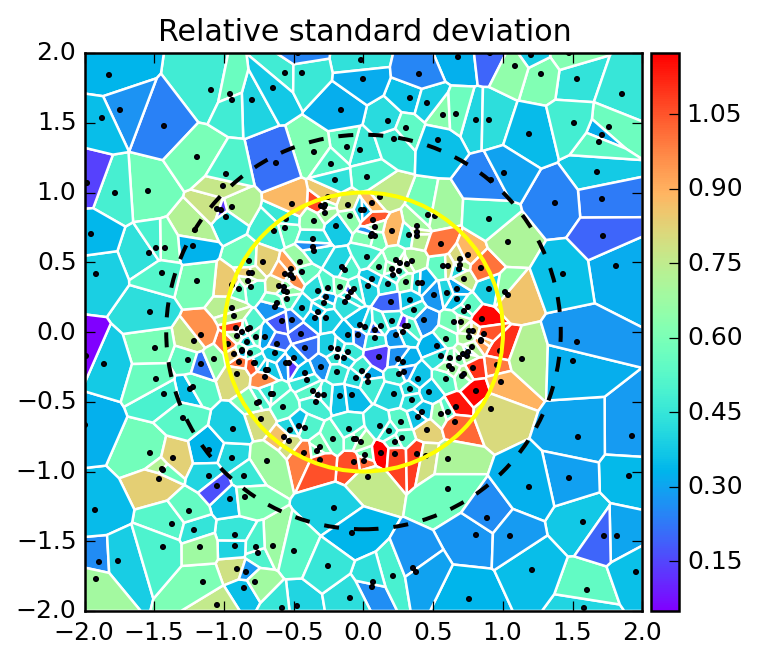
Figure 5: The analogue of Fig. 2 (left panel) and the analogue of the lower right panel in Fig. 3 (right panel), for the radially symmetric distribution (11). In order to keep the statistics the same as in Figs. 2 and 3 we place $N_{events}=280$ events inside the dashed circle with radius $r=\sqrt{2}$.

Just as in section 2.1.1, we choose $\rho=6$ and generate $N_{events}=280$ events according to (11); they are distributed so that the ratio of the bulk events on the two sides of the boundary is equal to $\rho$. Thus, out of the $N_{events}=280$ events inside the dashed circle with $r=\sqrt{2}$, on average we will have $\rho N_{events}/(\rho+1)=240$ events in the dense interior region (the unit circle) and $N_{events}/(\rho+1)=40$ events within the sparse exterior hollow disk.

In the left panel of Fig. 5, the brown-shaded polygons are by definition the edge cells (those crossed by the yellow circular boundary). The right panel in Fig. 5 demonstrates that, once again, the edge cells can be effectively selected by the RSD, $\bar{\sigma}_{i}$, of the areas of the neighboring cells.

2.2 Voronoi tessellations in three dimensions

Since the relevant physics example we treat in section 4 is in a three-dimensional phase space, $(m_{12},m_{23},m_{13})$, we shall now generalize our previous discussion to three dimensions. For this purpose, we consider the three-dimensional analogue of (11):

$$f(\vec{R})\sim\rho H(1-R)+H(R-1)H(\sqrt[3]{2}-R),$$ (12)

where now $\vec{R}=(x,y,z)$ is the position vector in three dimensions and $R\equiv|\vec{R}|$. The distribution, (12), again describes two regions of constant density, except now the dense region is a three-dimensional spherical core of radius 1. Again, we choose $\rho=6$ and generate $N_{events}=4200$ events according to (12). The events populate a ball of radius $R=\sqrt[3]{2}$ centered at the origin, $(x,y,z)=(0,0,0)$. On average, we expect to have $\rho N_{events}/(\rho+1)=3600$ events in the core and $N_{events}/(\rho+1)=600$ events in the outer hollow spherical shell ($1\leq R\leq\sqrt[3]{2}$).

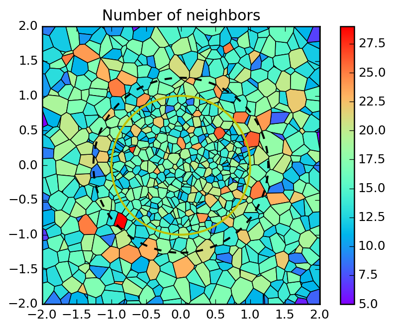
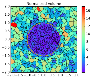
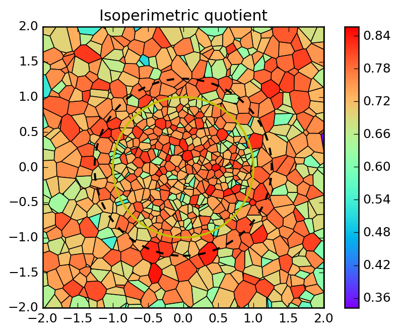
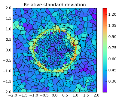
Figure 6: Two-dimensional slices at $z=0$ through phase space for the three-dimensional toy example studied in section 2.2. We distribute $N_{events}=4200$ points according to the three-dimensional probability distribution (12) within a sphere of radius $\sqrt[3]{2}$ centered at the origin $(x,y,z)=(0,0,0)$. The Voronoi tessellation is done before taking the two-dimensional slice, i.e., the cell boundaries seen on these four plots are obtained by intersecting the three-dimensional Voronoi cell boundaries with the plane at $z=0$. The yellow circle marks the boundary of the dense core. The resulting cells in the two-dimensional slice are color coded by a certain attribute of the corresponding three-dimensional Voronoi cell: number of neighbors (upper left); normalized volume (upper right); isoperimetric ratio (13) (lower left), and RSD of the neighboring volumes (1) (lower right).

Figs. 6 and 7 illustrate this three-dimensional simplified scenario in analogy to Figs. 3 and 4. Since the Voronoi cells in three dimensions are polyhedra, it is difficult to visualize them on a planar plot. Thus, Fig. 6 shows only a slice at a fixed $z=0$, i.e., an equatorial plane view. The cell boundaries seen in the figure are the intersections of the equatorial plane with the walls of the Voronoi polyhedra. The interiors of those cells are color-coded according to the value of the geometric property (number of faces, volume, etc.) of the corresponding three-dimensional polyhedron. For example, the upper left panel in Fig. 6 shows that the Voronoi polyhedra typically have a relatively large number of faces (or equivalently, neighbors); the corresponding distribution for bulk cells, shown in the upper left panel in Fig. 7, is known to peak at 15 Lorz1991 . We also observe that the edge cells are very similar in that regard, i.e., there is no appreciable difference in the number of neighbors as we move across the boundary.

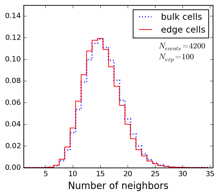
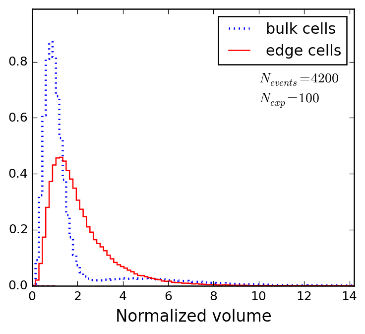
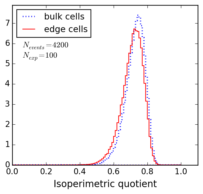
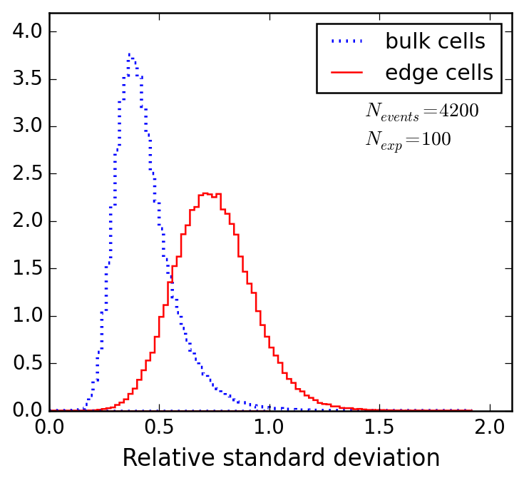
Figure 7: The same as Fig. 4, but for the three-dimensional toy example depicted in Fig. 6. Edge cells are defined to be those Voronoi cells which are crossed by the boundary of the unit sphere ($r=1$).

In the upper right panels of Figs. 6 and 7 we show the corresponding result for the normalized volumes, $\bar{v}_{i}$, of the Voronoi polyhedra, where, in analogy to (7), we scale each volume, $v_{i}$, by the expected average volume in the dense core, $\frac{4}{3}\pi(\rho+1)/(\rho N_{events})$. As expected, the distribution for bulk cells is bimodal, while edge cells behave somewhat similarly to the interior bulk cells (as we already saw in the two-dimensional example of section 2.1.1).

In the lower left panels of Figs. 6 and 7 we plot the analogous “isoperimetric quotient” for the three-dimensional case,

$$Q_{i}\equiv\frac{6\sqrt{\pi}\,v_{i}}{s_{i}^{3/2}},$$ (13)

where $v_{i}$ ($s_{i}$) is the volume (surface area) of the Voronoi polyhedron and the normalization is chosen so that $Q_{i}=1$ for a perfect sphere. Figs. 6 and 7 show that the shapes of the Voronoi polyhedra, as measured by (13), are very similar in the two bulk regions and not much different near the boundary either.

This leaves us with the RSD, $\bar{\sigma}_{i}$, of the volumes for the set of neighbors, $N_{i}$. This quantity was already defined in (1) and our results are shown in the lower right panels of Figs. 6 and 7. We see that $\bar{\sigma}_{i}$ can efficiently identify edge cells; the circular boundary is clearly seen in the lower right plot of Fig. 6. The $\bar{\sigma}_{i}$ distributions for bulk and edge cells are quite distinct, as shown in Fig. 7. Thus we verify that $\bar{\sigma}_{i}$ remains a promising variable for edge detection beyond the two-dimensional examples studied in Ref. Debnath:2015wra .

3 Phase Space Considerations

While two and three-body phase space is discussed at length in most standard lectures and textbooks on quantum field theory, a Lorentz-invariant formulation of the general case with an arbitrary number of final state particles is often omitted. This is in part because processes with more than three final state particles can, in almost all circumstances, be analyzed as a sequence of on-shell production and decay stages and in part because the level of formalism required to describe the general case is significantly more involved. Nevertheless, as was shown in Ref. Agrawal:2013uka , even when a cascade decay proceeds through multiple on-shell stages, treating the phase space in its fully-differential form captures important correlations that cannot be inferred from more traditional one-dimensional observables such as kinematic edges and endpoints. In this context, we briefly review the geometry of four-body phase space, concentrating on the equation describing the boundary of the kinematically available region and on the differential volume element. In section 3.2, we shall apply kinematic features obtained from the phase space considerations in section 3.1 to our uniform sphere example from section 2.2 and use the resulting toy example to study our Voronoi methods for three-dimensional data.

3.1 Review of the four-body phase space of a cascade decay

Let us consider the process where a heavy resonance, $X$, decays into four particles. We first focus on presenting the form of four-body phase space in full generality and will further specialize to the case where the decay proceeds via three-step two-body cascade decays as in Fig. 1. Following the argument in Ref. ByersYang , we begin by introducing a $4\times 4$ matrix defined as

$${\mathcal{Z}}=\left\{z_{ij}\right\}\quad{\rm with}\quad z_{ij}=p_{i}\cdot p_{j}\,,$$ (14)

where the $\{p_{i}\}$ denote four momenta of final state particles, including the NPP $X_{4}$. We then define the characteristic polynomial of $\mathcal{Z}$ as

$$\det\left[\lambda I_{4\times 4}-\mathcal{Z}\right]\equiv\lambda^{4}-\left(\sum_{i=1}^{4}\Delta_{i}\lambda^{4-i}\right)=0,$$ (15)

where $\lambda$ represents the relevant eigenvalues and the $\Delta_{i}$ identify the coefficients of the above polynomial. Specifically, one finds that $\Delta_{1}={\rm Tr}[{\mathcal{Z}}]=\sum_{i=1}^{4}m_{i}^{2}$ and $\Delta_{4}=-\det\left[{\mathcal{Z}}\right]$. It turns out that the kinematically allowed region is given by $\Delta_{1,2,3,4}>0$ ByersYang ; the boundary of this region is formed by

$$\Delta_{4}=0,\qquad\Delta_{1,2,3}>0\,.$$ (16)

What makes four-body (and higher) phase space particularly interesting is the form of the volume element. In terms of $m_{ij}^{2}=\left(p_{i}+p_{j}\right)^{2}=2z_{ij}+m_{i}^{2}+m_{j}^{2}$, the four-body phase space, $\Pi_{4}$, can be written as

$$d\Pi_{4}=\left(\prod_{i<j}dm_{ij}^{2}\right)\frac{8}{(4\pi)^{10}M_{X}^{2}\Delta_{4}^{1/2}}\ \delta\left(\sum_{i<j}m_{ij}^{2}-\left(M_{X}^{2}+2\sum_{i=1}^{4}m_{i}^{2}\right)\right),$$ (17)

where the normalization has been chosen to reproduce the PDG convention Agashe:2014kda for the well-known expression with non-Lorentz invariant quantities

$$d\Pi_{4}=\delta\left(p_{X}-\sum_{i=1}^{4}p_{i}\right)\prod_{i=1}^{4}\frac{d^{3}p_{i}}{(2\pi)^{3}2E_{i}}.$$ (18)

We remark that $d\Pi_{4}$ is inversely proportional to $\Delta_{4}$, and, given the fact that $\Delta_{4}=0$ defines the kinematic boundary, as in (16), the phase space has a singular structure near $\Delta_{4}=0$. While being an integrable singularity, this implies that events are more likely to be populated close to the boundary rather than far away from it. This observation is ideal for mass measurements which ultimately rely on the determination of this phase space boundary.

Given the generic formalism for the phase space with four particles in the final state, we now specialize to the case where the decay proceeds through the three consecutive two-body decays shown in Fig. 1. The $X_{i}$’s are NPPs represented by red dashed lines, while the $v_{i}$’s are SM particles represented by black solid lines. For simplicity, we assume that all SM particles are massless unless specified otherwise. $X_{1,2,3}$ are assumed to be narrow resonances, while $X_{4}$ is collider-stable and invisible.

We point out that the presence of the intermediate particles does not affect the enhancement near the boundary of phase space discussed above. Within the narrow width approximation, each internal propagator squared can be replaced by a delta function, whose argument is linear in the $z_{ij}$ or, equivalently, in the $m_{ij}^{2}$ variables. Therefore, integrating over those delta functions does not introduce any non-trivial Jacobian factors which would ruin the enhancement.

To quantify the enhancement near the boundary for this event topology, we derive the analytic form of the $\Delta_{4}$ probability distribution and show that it is completely independent of $m_{X_{i}}$ for the massless limit, i.e., $m_{v_{i}}=0$. We start by writing $\Delta_{4}$ in terms of the experimental observables $m_{v_{i}v_{j}}^{2}$ which are denoted by $m_{12}^{2}$, $m_{13}^{2}$, and $m_{23}^{2}$. These dimensionful variables can be traded for dimensionless, unit-normalized variables $\xi_{ij}$ as

$$m_{ij}^{2}\equiv\xi_{ij}\,m_{ij,{\rm max}}^{2},$$ (19)

where $0\leq\xi_{ij}\leq 1$ and the maximal values, $m_{ij,{\rm max}}^{2}$, are given by the well-known kinematic endpoint formulae (see, e.g., Allanach:2000kt ):

$$m_{12,{\rm max}}^{2} = \frac{(m_{X_{1}}^{2}-m_{X_{2}}^{2})(m_{X_{2}}^{2}-m_{X_{3}}^{2})}{m_{X_{2}}^{2}}\,,$$ (20)

$$m_{13,{\rm max}}^{2} = \frac{(m_{X_{1}}^{2}-m_{X_{2}}^{2})(m_{X_{3}}^{2}-m_{X_{4}}^{2})}{m_{X_{3}}^{2}}\,,$$ (21)

$$m_{23,{\rm max}}^{2} = \frac{(m_{X_{2}}^{2}-m_{X_{3}}^{2})(m_{X_{3}}^{2}-m_{X_{4}}^{2})}{m_{X_{3}}^{2}}\,.$$ (22)

We also trade the dimension-8 quantity $\Delta_{4}$ for a dimensionless and unit-normalized quantity $q$ defined as

$$\Delta_{4}\equiv q\,\Delta_{4,{\rm max}},\quad 0\leq q\leq 1.$$ (23)

Here the maximum value of $\Delta_{4}$ is given by

$$\Delta_{4,{\rm max}}=\left(\frac{(m_{X_{1}}^{2}-m_{X_{2}}^{2})(m_{X_{2}}^{2}-m_{X_{3}}^{2})(m_{X_{3}}^{2}-m_{X_{4}}^{2})}{8m_{X_{2}}m_{X_{3}}}\right)^{2}.$$ (24)

As shown in Ref. Agrawal:2013uka , for any given set of masses, $\left\{m_{X_{i}}\right\}$, in this topology, the probability of obtaining any given event near the point, $\left\{m_{ij}^{2}\right\}$, is expressed as

$$dP=\frac{1}{4\pi m_{X_{1}}^{2}}\left(1-\frac{m_{X_{2}}^{2}}{m_{X_{1}}^{2}}\right)^{-1}\left(1-\frac{m_{X_{3}}^{2}}{m_{X_{2}}^{2}}\right)^{-1}\left(1-\frac{m_{X_{4}}^{2}}{m_{X_{3}}^{2}}\right)^{-1}\frac{H\left(\Delta_{4}\right)}{\sqrt{\Delta_{4}}}dm_{12}^{2}\,dm_{13}^{2}\,dm_{23}^{2},$$ (25)

or equivalently, in terms of the dimensionless quantities, $\xi_{ij}$ and $q$, defined in (19) and (23), this can be rewritten as

$$dP=\frac{2}{\pi}\frac{m_{X_{3}}}{m_{X_{2}}}\frac{H\left(q\right)}{\sqrt{q}}d\xi_{12}\,d\xi_{13}\,d\xi_{23}.$$ (26)

Here $H(x)$ is the usual Heaviside step function.

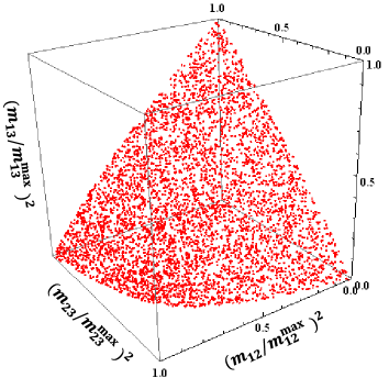
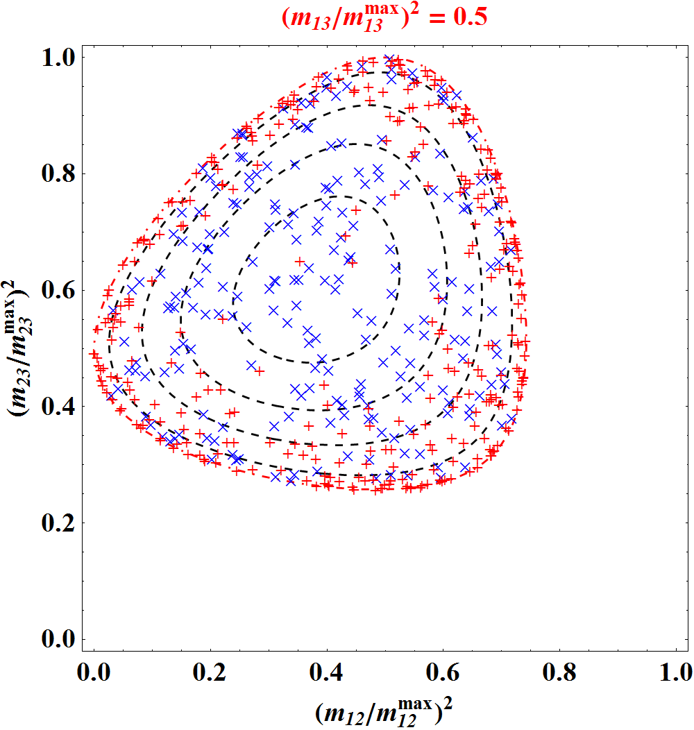
Figure 8: The phase space structure implied by eq. (25). The data points are generated with the event topology in Fig. 1, using a constant matrix element. The mass spectrum is $(m_{X_{1}},m_{X_{2}},m_{X_{3}},m_{X_{4}})=(500,350,200,100)$ GeV. A three-dimensional scatter plot (upper left) and three phase space slices at fixed $\xi_{13}$: $\xi_{13}=0.25$ (upper right), $\xi_{13}=0.5$ (lower left), and $\xi_{13}=0.75$ (lower right). The red dot-dashed (outermost) curve is the contour for $\Delta_{4}=0$, while the black dashed curves correspond to $\Delta_{4}$ contours for 10%, 30%, 50%, 70%, and 90% of $\Delta_{4,\max}$. The data points which would have emerged via the flat component in eq. (27) are represented by blue “$\times$” symbols, whereas the data points from the remaining enhanced component $\sim\frac{1}{\sqrt{q}}-1$ are represented by red “$+$” symbols.

Obviously, the expression in eq. (26) diverges for $q\rightarrow 0$, as expected from the general discussion earlier, and has a non-zero finite value at $q_{\max}=1$. In order to visualize the enhancement near $q\sim 0$, it is useful to partition the probability density in (26) into two components: a flat piece, proportional to $1$, and an enhanced piece, containing the $q^{-1/2}$ singularity:

$$\frac{dP}{dV_{\xi}}\sim\frac{1}{\sqrt{q_{\max}}}+\left(\frac{1}{\sqrt{q}}-\frac{1}{\sqrt{q_{\max}}}\right)=1+\left(\frac{1}{\sqrt{q}}-1\right),$$ (27)

where $dV_{\xi}\equiv d\xi_{12}\,d\xi_{23}\,d\xi_{13}$ is a shorthand notation. If events were uniformly distributed over the entire phase space in $\xi_{ij}$, their probability density would simply be proportional to the first (constant) term in eq. (27). Hence, all non-trivial effects in the phase space density distribution are due to the second term (inside the parentheses) in (27).

Fig. 8 helps us develop some useful intuition about the probability distribution (27). The upper left panel shows a scatter plot of physical events in the dimensionless $\xi_{ij}$-space, generated according to (27). We used a mass spectrum of $(m_{X_{1}},m_{X_{2}},m_{X_{3}},m_{X_{4}})=(500,350,200,100)$ GeV. The events populate a compact region whose shape has been likened to that of a “samosa” Kim:2015bnd . Since it is difficult to visualize the enhancement near the phase space boundary in this three-dimensional view, in the next three panels of Fig. 8 we take a few slices at fixed $\xi_{13}$: $\xi_{13}=0.25$ (upper right), $\xi_{13}=0.5$ (lower left), and $\xi_{13}=0.75$ (lower right). For each slice at a fixed $\xi_{13}$, we show all data points whose $m_{13}^{2}$ values fall within $0.5$ GeV² of the nominal value for that slice, i.e., within $\xi_{13}m_{13,max}^{2}\pm 0.5$ GeV². Then we project those points onto the plane of $\xi_{12}$ vs. $\xi_{23}$ and divide them into two (color-coded) groups. The data points which would have emerged from the flat piece in (27) are denoted with blue “$\times$” symbols, whereas the points arising from the enhanced piece in (27) are identified by red “$+$” symbols. In addition, we also show several theoretical contours of constant $\Delta_{4}$ values, starting with the outermost red dot-dashed curve at $\Delta_{4}=0$ (i.e., $q=0$) representing the phase space boundary. The internal, black dashed curves mark the contours for $\Delta_{4}=0.1\,\Delta_{4,\max}$, $\Delta_{4}=0.3\,\Delta_{4,\max}$, $\Delta_{4}=0.5\,\Delta_{4,\max}$, $\Delta_{4}=0.7\,\Delta_{4,\max}$, and $\Delta_{4}=0.9\,\Delta_{4,\max}$, respectively. Note that some of these contours are absent from the bottom panels because the relevant hyper-surfaces, corresponding to large $\Delta_{4}$ values do not intersect those slices.

Comparing the densities of red and blue data points, we get an idea about the effect of the enhancement in the vicinity of the phase space boundary. The blue points are more or less uniformly distributed, which is by design. In contrast, the distribution of red points is highly irregular, and their density peaks at the phase space boundary. For a more quantitative understanding, we derive the analytic expression for the probability density function in $q$ and obtain del4short

$$\frac{dP}{dq}=\frac{\arcsin(\sqrt{1-q})}{2\sqrt{q}}.$$ (28)

As previously advertised, this probability density function is completely independent of all $\left\{m_{X_{i}}\right\}$ and is enhanced near $q\approx 0$. In other words, the fraction of events that lie in a fixed $q$-interval is universal, and it is enhanced near the boundary of the phase space region. For example, roughly $5\%$ of events have $q\leq 10^{-3}$, i.e., less than 0.1% of $\Delta_{4,\max}$.

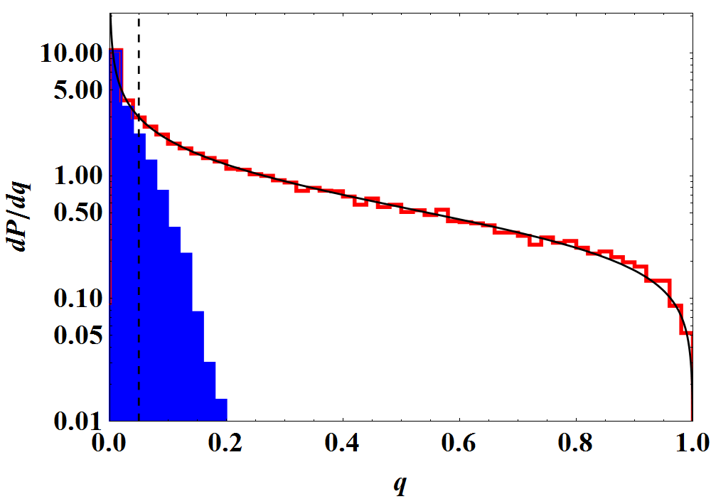
Figure 9: Probability density distribution in the $q$ variable (23) using the same event sample as in Fig. 8. The blue shaded histogram is contributed by the boundary data points which are tagged by the Voronoi tessellation. The black solid curve is the theory prediction for $dP/dq$ in eq. (28).

In Fig. 9, we plot the distribution of the $q$ variable from (23), taking 20,000 events out of the same event sample as the one used for Fig. 8. If we define any phase space point whose $q$ value is less than 5% of $q_{\max}$ as a boundary point, we find that $\sim 33\%$ of the events are then categorized as boundary points. The red histogram represents the $q$ distribution with respect to the full data set; the black dashed, vertical line denotes the location of $0.05\,q_{\max}$. The black solid curve shows the theoretical prediction from eq. (28). One can easily see that the $q$ distribution (red histogram) is fully consistent with the theory expectation. Indeed, the value of $q$ (or equivalently, $\Delta_{4}$) is not an experimental observable, since it requires a model assumption (the input of a mass spectrum for $X_{i}$). What is needed then is a practical way of tagging the boundary data points with such low values of $q$ by some other means; we employ Voronoi tessellations as an available tool. We Voronoi tessellate our phase space using the full data set. If a given Voronoi cell has vertices on both sides of the “samosa” surface defined by $q=0$ (or equivalently, $\Delta_{4}=0$), then the associated data point is tagged as a boundary point (recall the definition of “edge” cells in Fig. 2). The contribution from the boundary points extracted with the above algorithm is shown by the blue shaded histogram in Fig. 9, which we find represents $\sim 38\%$ of the events in the sample. As Fig. 9 demonstrates, the set of boundary cells which can be tagged by placing a cut on $q$ is essentially the same as the set of boundary cells identified with the Voronoi tessellation. In what follows, therefore, instead of using the variable $q$, which is experimentally inaccessible, we shall focus on the Voronoi cells belonging to the blue-shaded histogram in Fig. 9 and try to develop a tagging method based on their geometric properties, since they are experimentally observable.

3.2 Density-enhanced sphere boundaries

Inspired by the behavior of the phase space density near the boundary, we deform the density of data points from the sphere example considered previously in section 2.2. Performing Voronoi tessellations and studying the properties of the resulting Voronoi cells, we can develop our insight on what is expected from physical examples. Note that $\Delta_{4}$ vanishes on the phase space boundary and takes its maximum somewhere in the bulk. In other words, the $\Delta_{4}$ value increases as the distance between the data point of interest and the boundary surface increases (see also contours in Fig. 8). Although specifying the value of distance does not determine the $\Delta_{4}$ value, it turns out that there exists a positive correlation between the two quantities del4short . To proceed, we make the simplifying Ansatz that the distribution of the data points inside a unit sphere depends only on the radius, $R$, with an enhancement at $R=1$. Motivated by the form of the probability density in (26), we introduce the following volume density function for the data points inside the unit sphere

$$\frac{dP}{dV}\sim\frac{1}{\sqrt{1-R}}\,.$$ (29)

Now in analogy to (12), we consider the three-dimensional distribution

$$f(\vec{R})\sim\frac{\rho}{\sqrt{1-R}}H(1-R)+H(R-1)H(\sqrt[3]{2}-R).$$ (30)

Following the example from section 2.2, we again take the density ratio $\rho=6$ and generate $N_{events}=4200$ events according to (30). Our results are shown in Figs. 10 and 11, which are the analogues of Figs. 6 and 7, respectively.

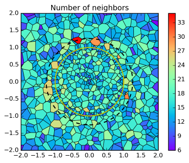
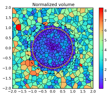
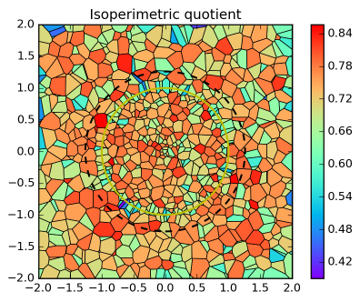
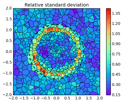
Figure 10: The same as Fig. 6, but for a toy example in which the dense core has a non-uniform distribution given by (30).

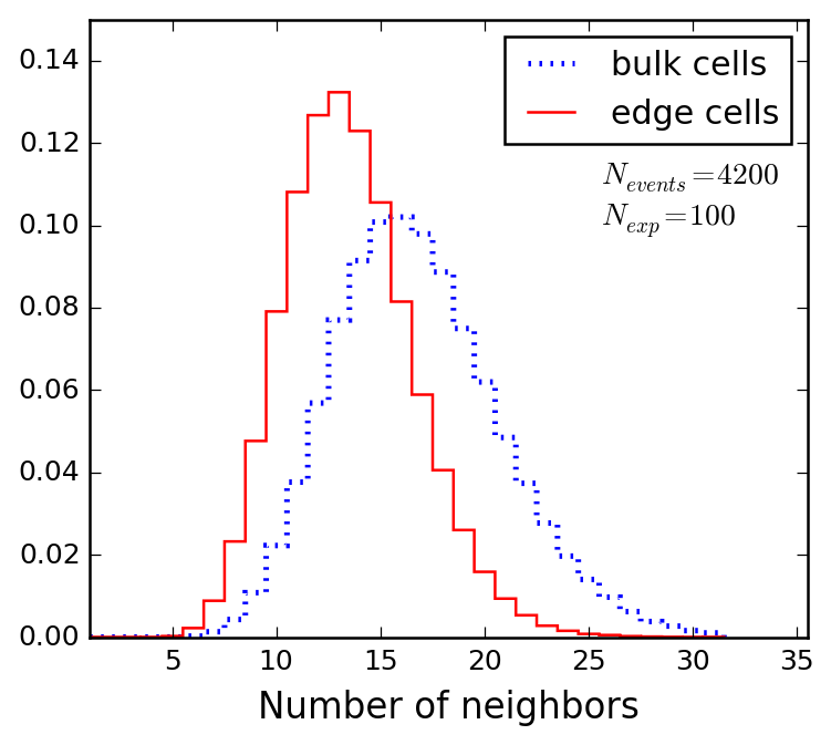
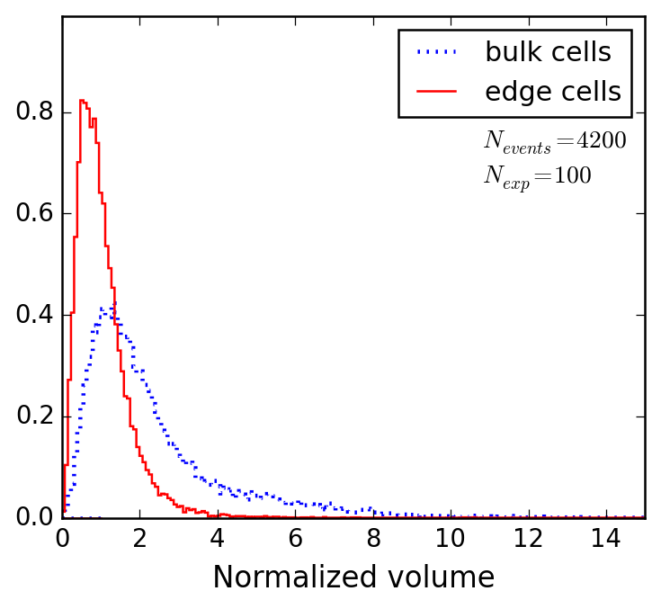
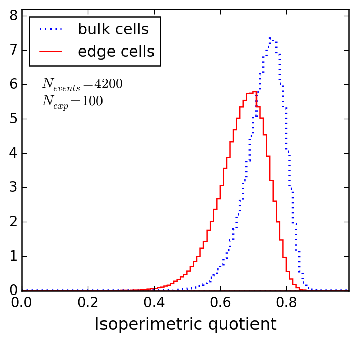
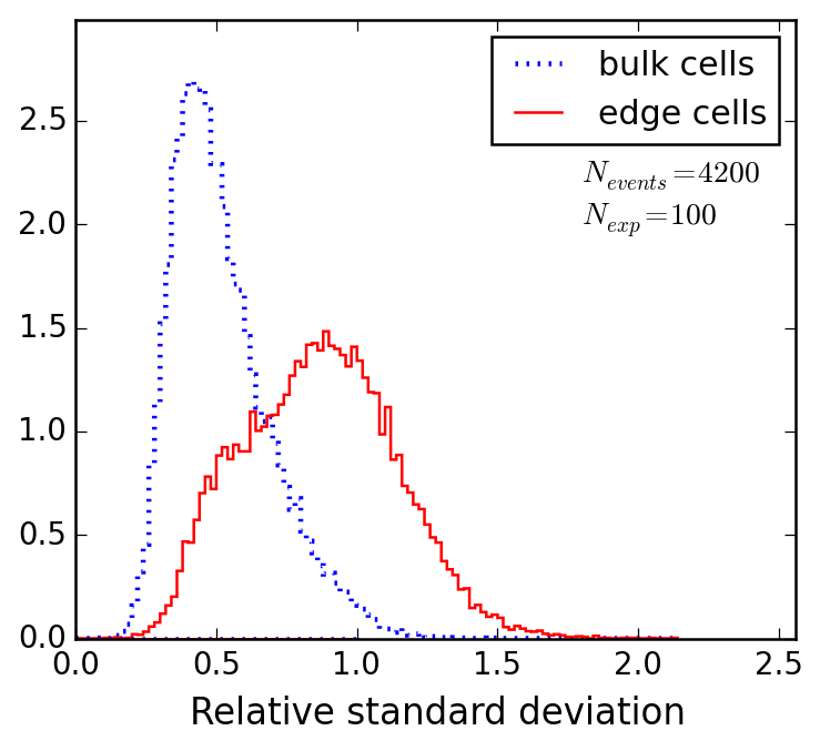
Figure 11: The same as Fig. 7, but for the example shown in Fig. 10.

We see that, in principle, all four variables plotted in Fig. 10 show some potential for discriminating edge cells. For example, a careful inspection of the lower left panel of Fig. 10 reveals that the edge cells appear somewhat elongated, which results in a lower isoperimetric quotient, as confirmed by the lower left panel in Fig. 11. On the other hand, due to the density enhancement near the boundary, we would also expect the edge cells to have smaller normalized volumes. This expectation is also confirmed — in the upper right panels of Figs. 10 and 11. Finally, the lower right panels of Figs. 10 and 11 again demonstrate that the RSD of the neighboring areas is a good discriminator, in agreement with our observations from the earlier toy examples. In order to compare the performance of the four variables investigated in Figs. 10 and 11, we use the concept of a ROC curve, which is reviewed in Appendix A.

3.3 Finding density-enhanced sphere boundaries with Voronoi tessellations

We now analyze the example of a sphere with an enhanced density near the boundary considered in section 3.2, in terms of ROC curves. In the left panel of Fig. 12, we show the ROC curve for each of the four variables depicted in Figs. 10 and 11: number of neighbors (magenta dotted line), normalized volume (green dashed line), isoperimetric quotient (blue dot-dashed line) and RSD of neighbor areas (red solid line). We observe that the RSD outperforms the other three variables, in agreement with the conclusions from Debnath:2015wra for the two-dimensional case.

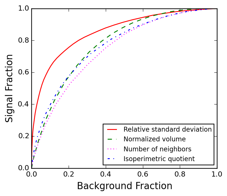
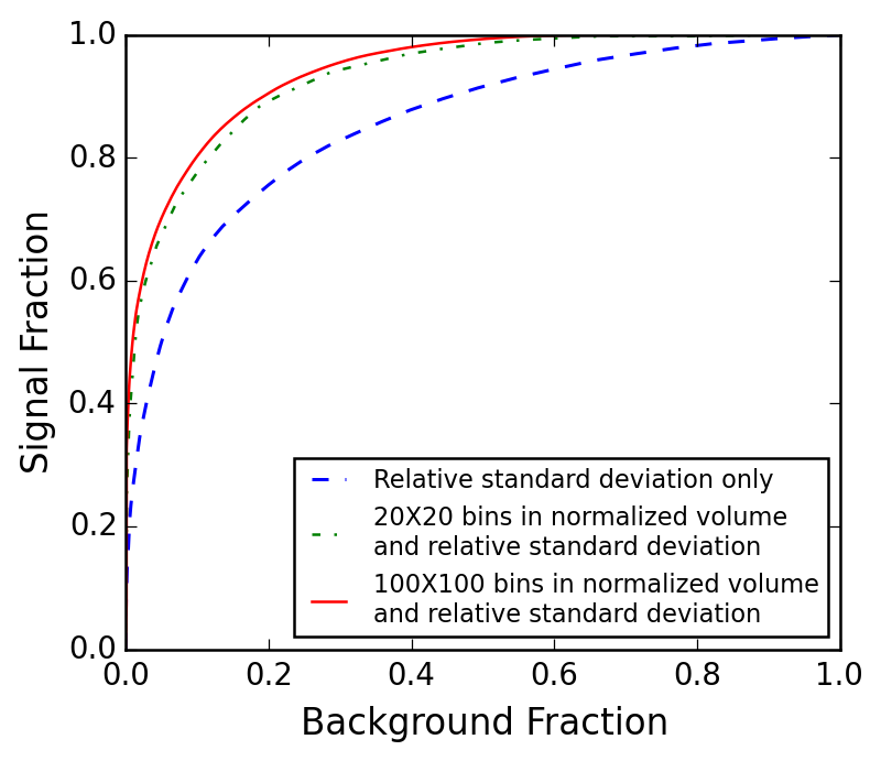
Figure 12: ROC curves for the toy example depicted in Fig. 10. Left: The four different ROC curves resulting from each of the four variables shown in Fig. 11. Right: Improved ROC curves with optimal two-dimensional cuts in the $(\bar{v},\bar{\sigma})$ plane as illustrated in Fig. 13: with $20\times 20$ binning (green dot-dashed) or $100\times 100$ binning (dotted blue). The blue dashed line is the ROC curve based on the $\bar{\sigma}$ variable alone and is identical to the solid red line in the left panel.

However, the other three variables also have a certain degree of discriminating power, as seen in Fig. 11. The natural question then is how much additional sensitivity can be gained by considering not just one, but two variables simultaneously. We studied the correlations between the RSD, $\bar{\sigma}$, and each of the other three variables, and generally find that they are not perfectly correlated. (This makes sense intuitively because the RSD is computed from the neighbor set, $N_{i}$, while the other three variables are properties of the individual cell.) We concluded that, among the three options, the normalized volume, $\bar{v}$, is the most promising, since it appears least correlated with $\bar{\sigma}$. Therefore, we expect that the sensitivity will improve once we incorporate the normalized volume, $\bar{v}$, in the analysis. This expectation is confirmed in the right panel of Fig. 12, where we show “improved” ROC curves based on binning in both $\bar{v}$ and $\bar{\sigma}$. The procedure, illustrated in Fig. 13, is as follows. We consider the $(\bar{v},\bar{\sigma})$ plane divided into $20\times 20$ bins (left panel of Fig. 13) or $100\times 100$ bins (right panel of Fig. 13). We expect the signal, i.e., the boundary Voronoi cells, to populate the bins with small volume and relatively large RSD, while the background, i.e., the bulk cells, are distributed more uniformly throughout the $(\bar{v},\bar{\sigma})$ plane. In order to build the optimal ROC curve, we need to determine the signal to background ratio, $S/B$, in each bin, and design the cuts so that we remove successively the bins with the smallest $S/B$. The bins in Fig. 13 are color-coded according to the corresponding value of $\log(S/B)$. Given the finite statistics, there are bins which have no events (neither signal nor background); they are left uncolored. For definiteness, the bins which have some signal events, but no background events, are assigned the same value as the maximal $\log(S/B)$ value among the bins containing both signal and background events. Similarly, the bins which had some background events, but no signal events, were assigned the same value as the minimal $\log(S/B)$ value among the bins containing both signal and background events.

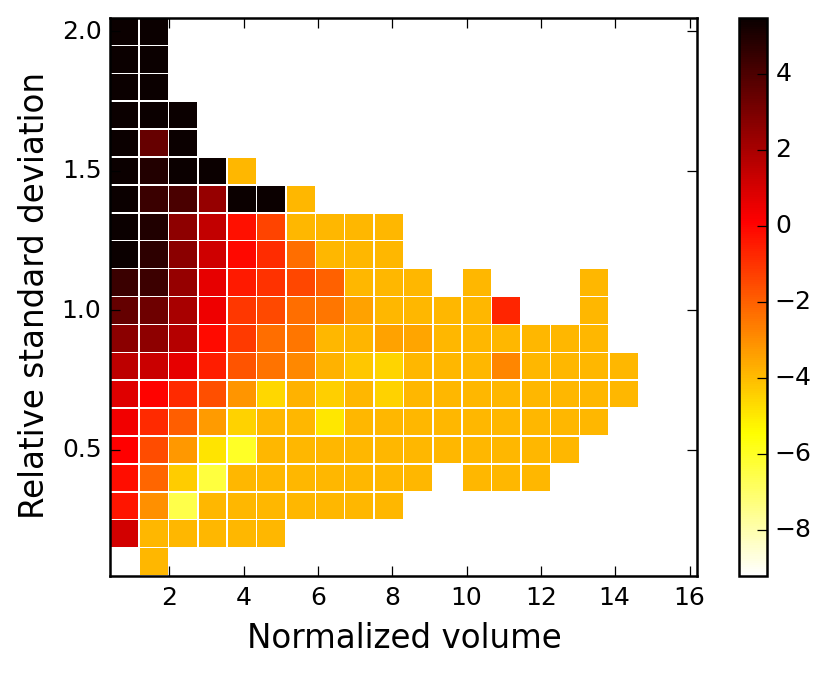
Figure 13: Two-dimensional histograms of the expected signal to background ratio in the $(\bar{v},\bar{\sigma})$ plane: for $20\times 20$ bin (left) and $100\times 100$ bins (right). The ROC curves in the right panel of Fig. 12 were built by successively cutting away the bin with the lowest signal-to-background ratio among all remaining bins. (Alternatively, one could start from zero and successively keep adding the bin with the highest signal-to-background ratio among all remaining bins.)

Fig. 13 shows that, as expected, the bins with the largest $S/B$ (colored in black) are located in the upper left corner of the plot, corresponding to small $\bar{v}$ and large $\bar{\sigma}$. The spread in the cluster of black-colored bins is indicative of the gain in sensitivity due to simultaneous consideration of the two variables, $\bar{v}$ and $\bar{\sigma}$. According to the right panel of Fig. 12, the bulk of the gain is already obtained with a $20\times 20$ grid; increasing the number of bins 25 times to a $100\times 100$ grid does not lead to substantial improvement. Therefore, in practice, one might want to consider grids of even smaller size, especially since the true ranking of the bins in terms of $S/B$ depends on the parameter values, e.g., the density enhancement on the boundary and the value of $\rho$, which are not known a priori. This is why when we consider the physics example in the next section, we shall utilize a smaller grid of $15\times 15$ bins in the $(\bar{v},\bar{\sigma})$ plane (see Fig. 16).

4 Finding Phase Space Boundaries with Voronoi Tessellations

We now use Voronoi tessellations to find the phase space boundary for SUSY events at the $14$ TeV LHC. We consider the $2+2+2$ topology from Fig. 1, where, as usual, a (left-handed) squark $X_{1}=\tilde{q}$ undergoes a cascade decay through a heavy neutralino, $X_{2}=\tilde{\chi}^{0}_{2}$; a slepton, $X_{3}=\tilde{\ell}$; and a light neutralino, $X_{4}=\tilde{\chi}^{0}_{1}$. As in Ref. Agrawal:2013uka , we consider the production of a squark in association with a neutralino LSP ($\tilde{\chi}^{0}_{1}$). Events were generated with MadGraph5 Alwall:2011uj . The mass spectrum that we used was $m_{\tilde{q}}=350$ GeV, $m_{\tilde{\chi}^{0}_{2}}=300$ GeV, $m_{\tilde{\ell}}=250$ GeV, and $m_{\tilde{\chi}^{0}_{1}}=200$ GeV. The particles visible in the detector are: a quark jet $v_{1}=j$, a “near” lepton $v_{2}=\ell_{n}$, and a “far” lepton $v_{3}=\ell_{f}$. The relevant phase space is then $(m_{12},m_{23},m_{13})\equiv(m_{j\ell_{n}},m_{\ell\ell},m_{j\ell_{f}})$. For SUSY signal events, each of these three variables exhibits an upper kinematic endpoint. The three endpoint values are given by eqs. (20-22):

$$m^{2}_{j\ell_{n},max} = 9931\ {\rm GeV}^{2},$$ (31)

$$m^{2}_{\ell\ell,max} = 9900\ {\rm GeV}^{2},$$ (32)

$$m^{2}_{j\ell_{f},max} = 11700\ {\rm GeV}^{2}.$$ (33)

From the three-dimensional point of view, the signal events populate the interior of a compact region in the $(m_{j\ell_{n}},m_{\ell\ell},m_{j\ell_{f}})$ space, whose boundary is given by the constraint Costanzo:2009mq ; Kim:2015bnd

$$\hat{m}^{2}_{j\ell_{f}}=\left[\sqrt{\hat{m}^{2}_{\ell\ell}\left(1-\hat{m}^{2}_{j\ell_{n}}\right)}\pm\frac{m_{\tilde{\ell}}}{m_{\tilde{\chi}^{0}_{2}}}\sqrt{\hat{m}^{2}_{j\ell_{n}}\left(1-\hat{m}^{2}_{\ell\ell}\right)}\right]^{2},$$ (34)

which, for convenience, is written in terms of unit-normalized variables (see also (19))

$$\hat{m}_{j\ell_{n}} = \frac{m_{j\ell_{n}}}{m_{j\ell_{n},max}},$$ (35)

$$\hat{m}_{\ell\ell} = \frac{m_{\ell\ell}}{m_{\ell\ell,max}},$$ (36)

$$\hat{m}_{j\ell_{f}} = \frac{m_{j\ell_{f}}}{m_{j\ell_{f},max}}.$$ (37)

Our main goal in this section will be to test the algorithms from the previous sections for tagging the Voronoi cells in the vicinity of the boundary surface (34). In addition to the signal events from squark-neutralino associated production with the squark decaying as in Fig. 1, we shall also consider a representative number of background events. In order to make contact with the results from the previous sections, in section 4.1 we first take the background events to be uniformly distributed in mass-squared phase-space, and we ignore the combinatorial background. Then in section 4.2 we study a more realistic case, where the SM background is comprised of dilepton $t\bar{t}$ events and we also account for the combinatorial problem with the two leptons.

4.1 An example with uniform background and no combinatorics

As in the other two three-dimensional examples considered in sections 2.2 and 3.3, in this section we include “SM physics background” events, which we take to be uniformly distributed everywhere throughout the mass-squared phase-space $(m^{2}_{j\ell_{n}},m^{2}_{\ell\ell},m^{2}_{j\ell_{f}})$ and normalized so that the density contrast across the boundary (34) is equal to $\rho=4$. Note that in this scenario the interior “bulk” events and the “edge” cells on the surface boundary (34) consist of both SUSY signal and SM background events.

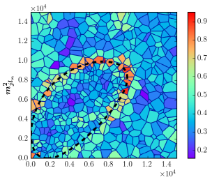
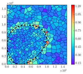
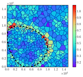
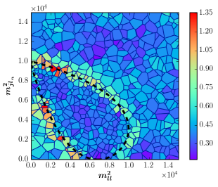
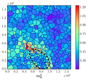
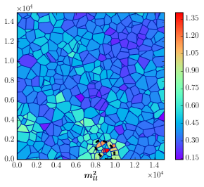
Figure 14: Two-dimensional slices of the relevant three-dimensional phase space of the SUSY-like cascade decay in Fig. 1. Each slice is in the $(m_{\ell\ell}^{2},m_{j\ell_{n}}^{2})$ plane at a fixed value of $m_{j\ell_{f}}^{2}=2000$ ${\rm GeV}^{2}$ (upper left panel); $m_{j\ell_{f}}^{2}=4000$ ${\rm GeV}^{2}$ (upper middle panel); $m_{j\ell_{f}}^{2}=6000$ ${\rm GeV}^{2}$ (upper right panel); $m_{j\ell_{f}}^{2}=8000$ ${\rm GeV}^{2}$ (lower left panel); $m_{j\ell_{f}}^{2}=10000$ ${\rm GeV}^{2}$ (lower middle panel); and $m_{j\ell_{f}}^{2}=11000$ ${\rm GeV}^{2}$ (lower right panel). As in Figs. 6 and 10, the two-dimensional cells seen in the plots result from the intersection of the projective plane with the three-dimensional Voronoi cells, and are color-coded by the value of $\bar{\sigma}_{i}$ for the corresponding three-dimensional Voronoi cell.

As before, we visualize the resulting Voronoi tessellation by presenting two-dimensional slices of the relevant three-dimensional phase space, in this case $(m^{2}_{j\ell_{n}},m^{2}_{\ell\ell},m^{2}_{j\ell_{f}})$. In Figs. 14 and 15 we show six slices in the $(m_{\ell\ell}^{2},m_{j\ell_{n}}^{2})$ plane at a fixed value of $m^{2}_{j\ell_{f}}$ as follows: $m_{j\ell_{f}}^{2}=2000$ ${\rm GeV}^{2}$ (upper left panel); $m_{j\ell_{f}}^{2}=4000$ ${\rm GeV}^{2}$ (upper middle panel); $m_{j\ell_{f}}^{2}=6000$ ${\rm GeV}^{2}$ (upper right panel); $m_{j\ell_{f}}^{2}=8000$ ${\rm GeV}^{2}$ (lower left panel); $m_{j\ell_{f}}^{2}=10000$ ${\rm GeV}^{2}$ (lower middle panel); $m_{j\ell_{f}}^{2}=11000$ ${\rm GeV}^{2}$ (lower right panel). As in Figs. 6 and 10, the two-dimensional cells seen in the plots result from the intersection of the projective plane with the three-dimensional Voronoi cells and are color-coded by the value of the RSD, $\bar{\sigma}_{i}$, defined in (1) (in Fig. 14) or the normalized volume $\bar{v}_{i}$ defined in (3) (in Fig. 15) of the corresponding three-dimensional Voronoi cell.

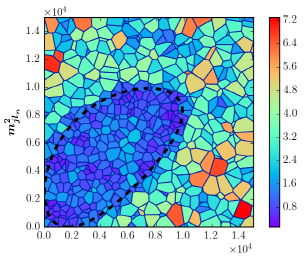
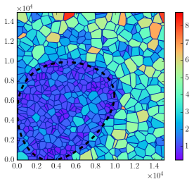
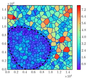
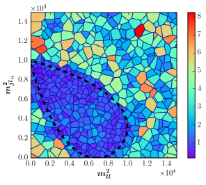
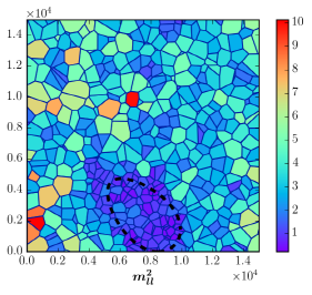
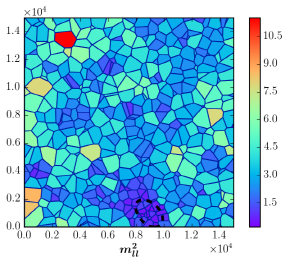
Figure 15: The same as Fig. 14, but color-coding the cells according to the normalized volume, $\bar{v}_{i}$, defined in (3).

Just as in the case of the density-enhanced sphere considered in section 3.3, Figs. 14 and 15 suggest that the edge cells near the phase space boundary (34) are characterized both by a large value of $\bar{\sigma}_{i}$ and a small value of $\bar{v}_{i}$. Therefore, in designing a selection cut to pick up edge cells, it makes sense to consider both of these two variables at the same time. This is illustrated in the left panel of Fig. 16, which is the analogue of Fig. 13 for this case.

Figure 16: The integer ranking of the $15\times 15$ bins in the $(\bar{v},\bar{\sigma})$ plane according to their signal-to-background ratio. Left: The ranking for the case of $\rho=4$. Right: the average ranking for the cases of $\rho=1.2$, $\rho=1.5$, $\rho=2.0$, $\rho=3.0$, and $\rho=4.0$.

We consider a moderately large $15\times 15$ grid in the $(\bar{v},\bar{\sigma})$ plane and rank the resulting bins according to their signal-to-background ratio as follows. The bin with the highest $S/B$ is assigned rank $1$, while the bin with the lowest $S/B$ is assigned rank $15\times 15=225$. In case of a tie between several bins, each bin is assigned the same average rank. Finally, bins with no events at all are ranked at the very bottom. We observe that, similarly to Fig. 13, the highest ranked bins in terms of $S/B$ appear at large values of $\bar{\sigma}$ and small values of $\bar{v}$. Using the obtained bin ranking, we can build the corresponding ROC curve, shown with the red solid line in the left panel of Fig. 17, which in some sense is the “ideal” ROC curve that could be achieved, if $\bar{\sigma}$ and $\bar{v}$ were the only discriminating variables under consideration.

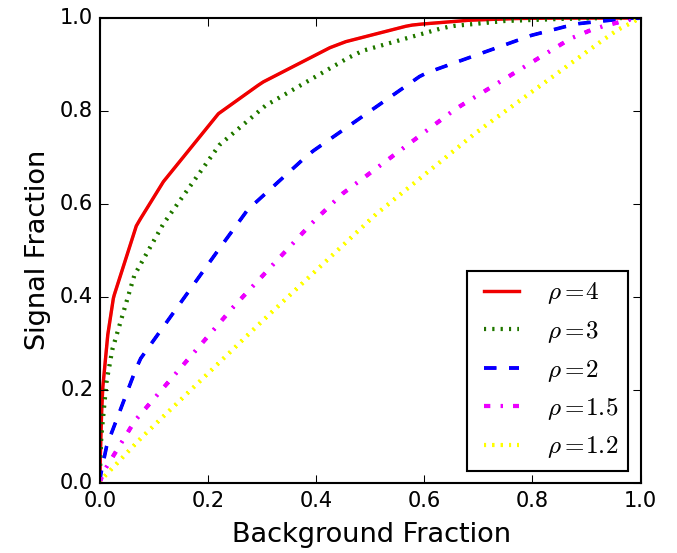
Figure 17: The same as the ROC curves shown in the right panel of Fig. 12, but for a $15\times 15$ grid. Left: the ranking of the bins in constructing the ROC curve was done with the correct value of $\rho$ (shown on each curve) used in generating the “data”. Right: the ranking of the bins was always done according to the “average” ranking shown in the right panel of Fig. 16.

One can now repeat the same procedure for different values of $\rho$. We show four more examples in the left panel of Fig. 17, with increasingly pessimistic values for the density contrast $\rho$: $3$, $2$, $1.5$ and $1.2$. As expected, the ROC curves become progressively worse, as quantified in the figure. With regards to the bin ranking in each case, we notice the following trend — the highest ranked bins remain at the lowest possible values of $\bar{v}$, but slide down the $\bar{\sigma}$ axis to slightly lower values of the RSD, near, or even below $\bar{\sigma}\sim 1$. This is easy to understand intuitively — as $\rho$ is decreased, the number densities on both sides of the surface boundary become more similar, and there is less variation between the sizes of bulk cells on the inside and on the outside. The fact that the bin ranking derived from our Monte Carlo simulations depends on the value of $\rho$ poses an important conceptual problem with this procedure — when the analysis is performed on real data, we will not know the actual value of $\rho$, and, hence, we will not be certain which particular ordering of bins to use. Nevertheless, the fact that the highest ranked bins are clustered, more or less, in the same location, suggests a possible resolution: we can simply average our results obtained for several different values of $\rho$ and use the resulting average rank for each bin, which is shown in the right panel of Fig. 16. The corresponding ROC curves derived with the help of this “average” bin ranking procedure are shown in the right panel of Fig. 17. Comparing the two panels of Fig. 17, we see that the ROC curves based on the average ranking are only slightly degraded compared to the “ideal” case.

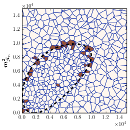
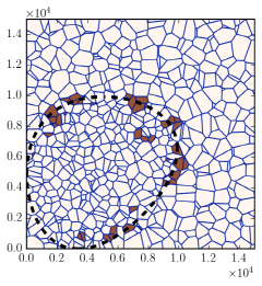
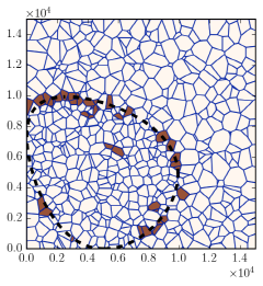
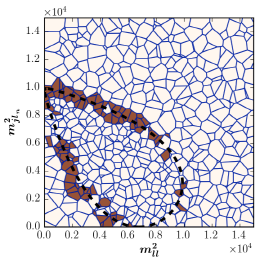
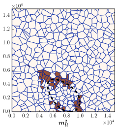
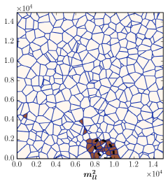
Figure 18: The Voronoi cells which pass the two-dimensional selection cut requiring the cell to belong to one of the top 5 bins in terms of signal-to-background ratio for the correct choice of $\rho=4$ (see the left panel in Fig. 16).

We are now ready to start designing selection cuts for the edge cells. One possibility is to select the cells which fall into the a predetermined number, $N_{top\ bins}$, of the highest ranked bins in the $(\bar{v},\bar{\sigma})$ plane. If we “cheat”, i.e., use the correct value of $\rho$ for the ranking (as in the left panel of Fig. 16), we obtain the result shown in Fig. 18, where we have chosen $N_{top\ bins}=5$. In general, the tagged cells are distributed throughout the volume of the three dimensional phase space, so for illustration purposes we again use the same six two-dimensional slices as in Figs. 14 and 15. We observe that the procedure is pretty efficient in tagging edge cells, and occasionally we tag an isolated bulk cell. Of course, for such a low value of $N_{top\ bins}$, not all edge cells will pass the cut, which will cause the boundary contours (marked with black dashed lines) to appear segmented and incomplete. By increasing the value of $N_{top\ bins}$, we can obviously tag more edge cells and eventually “close” those contours, but at the cost of more mistagged bulk cells.

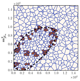
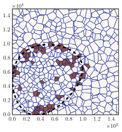
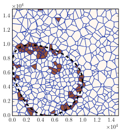
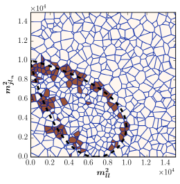
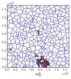
Figure 19: The same as Fig. 18, but using the average ranking of the bins shown in the right panel of Fig. 16.

Since the true value of $\rho$ will be unknown, the plots in Fig. 18 are for academic purposes only. The more realistic situation is depicted in the analogous Fig. 19, where we again choose $N_{top\ bins}=5$, only this time we use the average bin ranking from the right panel of Fig. 16. The result in Fig. 19 is slightly worse than Fig. 18 — while we do find a higher rate for mistagging bulk cells (typically in the interior), the majority of the tagged cells are very close to the surface boundary, suggesting that this is a promising technique for identifying edge cells.

4.2 A realistic example with $t\bar{t}$ background and combinatorics

We now repeat the exercise from the previous section 4.1 with two improvements. First, we have to address the combinatorial problem of distinguishing the “near” and “far” lepton. The standard approach in the literature is to trade the original variables $m_{j\ell_{n}}$ and $m_{j\ell_{f}}$ for the ordered pair Allanach:2000kt ; Gjelsten:2004ki ; Matchev:2009iw

$$m_{j\ell}(high) \equiv\max\left\{m_{j\ell_{n}},m_{j\ell_{f}}\right\},$$ (38a)

$$m_{j\ell}(low) \equiv\min\left\{m_{j\ell_{n}},m_{j\ell_{f}}\right\}.$$ (38b)

This reordering procedure is pictorially illustrated with the first two rows of plots in Fig. 20, where we show scatter plots of signal events for different ranges of the third invariant mass variable (the dilepton mass): $1,000\ {\rm GeV}^{2}\leq m_{\ell\ell}^{2}\leq 3,000\ {\rm GeV}^{2}$ (first column); $3,000\ {\rm GeV}^{2}\leq m_{\ell\ell}^{2}\leq 5,000\ {\rm GeV}^{2}$ (second column); $5,000\ {\rm GeV}^{2}\leq m_{\ell\ell}^{2}\leq 7,000\ {\rm GeV}^{2}$ (third column); and $7,000\ {\rm GeV}^{2}\leq m_{\ell\ell}^{2}\leq 9,000\ {\rm GeV}^{2}$ (fourth column).

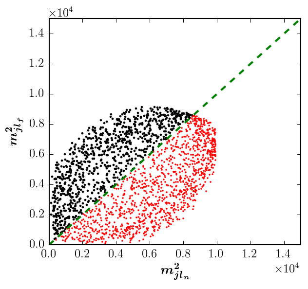
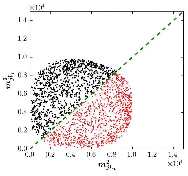
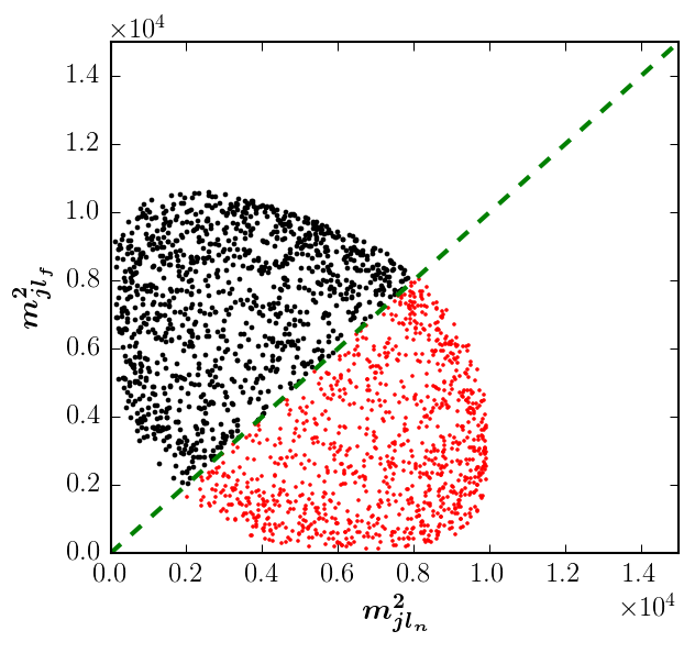
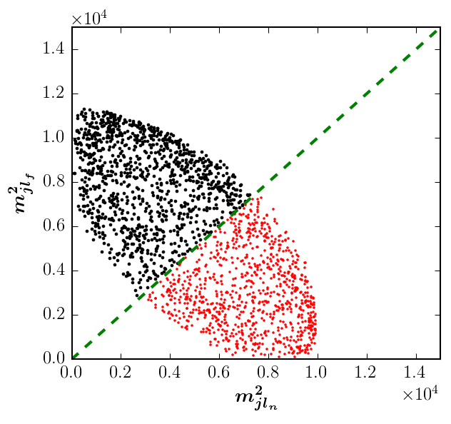
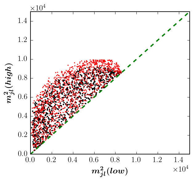
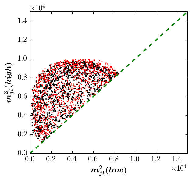
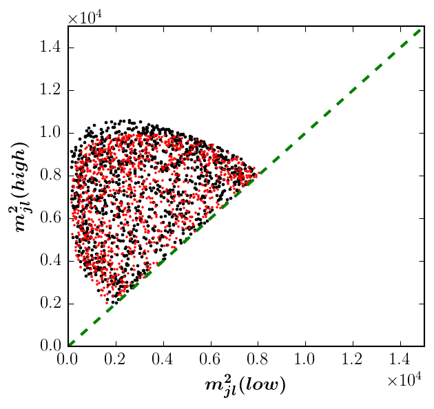
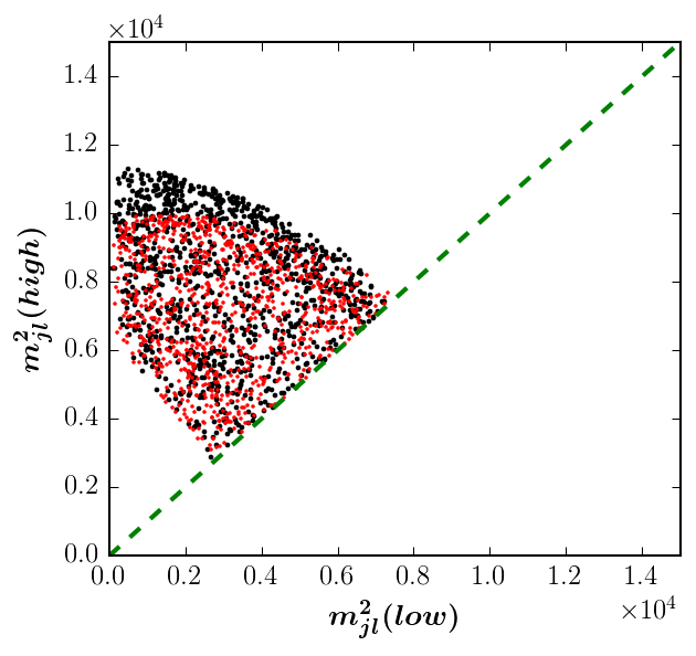
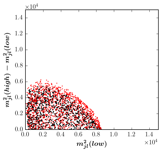
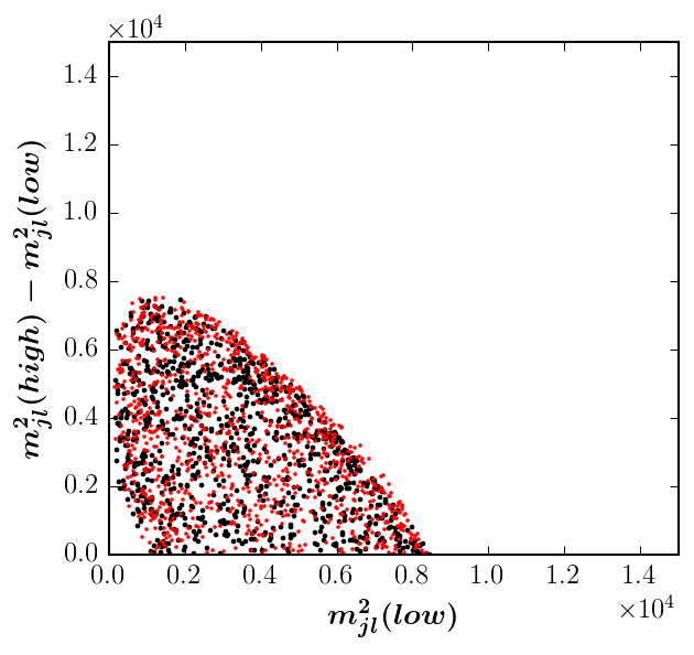
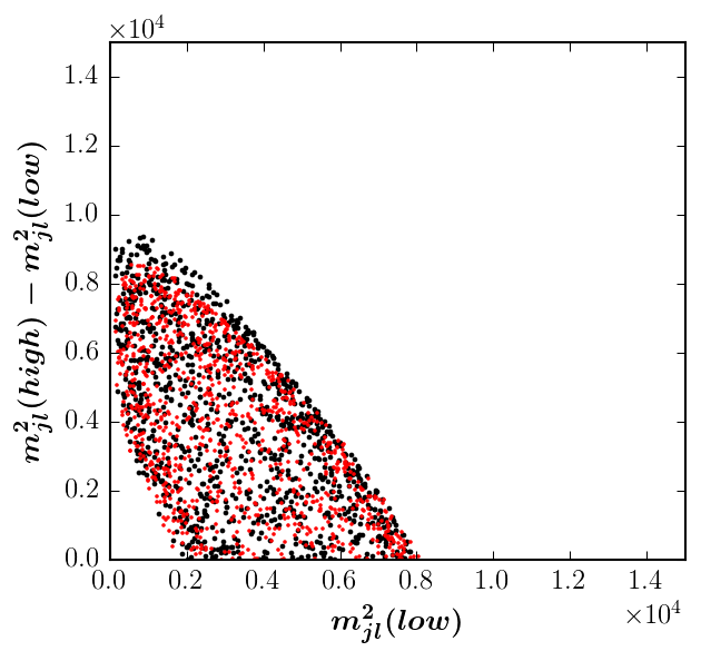
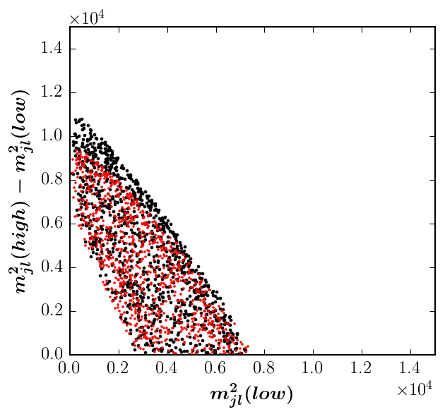
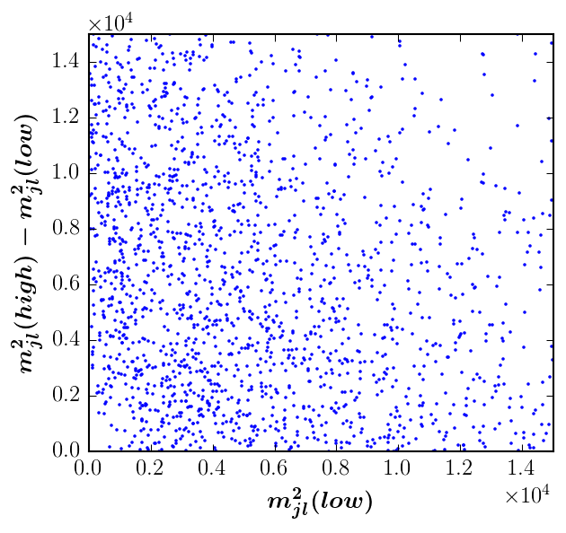
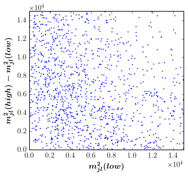
Figure 20: Scatter plots of signal events (black and red points, top three rows) and dilepton $t\bar{t}$ events (blue points, bottom row), for different ranges of the dilepton invariant mass squared: $1,000\ {\rm GeV}^{2}\leq m_{\ell\ell}^{2}\leq 3,000\ {\rm GeV}^{2}$ (first column); $3,000\ {\rm GeV}^{2}\leq m_{\ell\ell}^{2}\leq 5,000\ {\rm GeV}^{2}$ (second column); $5,000\ {\rm GeV}^{2}\leq m_{\ell\ell}^{2}\leq 7,000\ {\rm GeV}^{2}$ (third column); and $7,000\ {\rm GeV}^{2}\leq m_{\ell\ell}^{2}\leq 9,000\ {\rm GeV}^{2}$ (fourth column). In the first row, the signal events are plotted in the plane of $(m^{2}_{j\ell_{n}},m^{2}_{j\ell_{f}})$ and colored red (black) if $m^{2}_{j\ell_{n}}\geq m^{2}_{j\ell_{f}}$ ($m^{2}_{j\ell_{n}}\leq m^{2}_{j\ell_{f}}$). The same points are then plotted in the planes of $(m^{2}_{j\ell}(low),m^{2}_{j\ell}(high))$ (second row) and $(m^{2}_{j\ell}(low),m^{2}_{j\ell}(high)-m^{2}_{j\ell}(low))$ (third row). The background events in the fourth row are plotted in the plane of $(m^{2}_{j\ell}(low),m^{2}_{j\ell}(high)-m^{2}_{j\ell}(low))$.

In the first row, the signal events are plotted in the original plane of $(m^{2}_{j\ell_{n}},m^{2}_{j\ell_{f}})$, and the points are color-coded as follows. The points below the diagonal $45^{\circ}$ line, which have $m^{2}_{j\ell_{n}}\geq m^{2}_{j\ell_{f}}$, are colored in red, while the remaining points above the diagonal $45^{\circ}$ line with $m^{2}_{j\ell_{n}}\leq m^{2}_{j\ell_{f}}$, are colored in black. The same data is then plotted in the second row of Fig. 20 in the plane of $(m^{2}_{j\ell}(low),m^{2}_{j\ell}(high))$. Notice that the effect of the reordering procedure (38) is to leave all the black points in place, while interchanging the $x$ and $y$ coordinates of the red points. After the reordering (38), half of the plane on each plot is left blank. In order to avoid such voids, in the third row of Fig. 20 we replot the data in the plane of $(m^{2}_{j\ell}(low),m^{2}_{j\ell}(high)-m^{2}_{j\ell}(low))$, which is fully accessible.

As expected, the scatter plots in the third row of Fig. 20 exhibit boundary lines, which we can target with our edge-detecting method. In fact, each plot has two such boundaries where the signal number density sharply changes — one for the red points and another for the black points. At low values of $m_{\ell\ell}$ the “red” (“black”) boundary line is an external (internal) boundary, while for high values of $m_{\ell\ell}$ it is the other way around. At intermediate values of $m_{\ell\ell}$ the two boundaries are very close to each other and that is where we expect the edge detection method to perform best.

Having thus taken care of the combinatorial problem, we now also improve our treatment of the background — instead of uniformly distributed background events as in section 4.1, we consider dilepton events from $t\bar{t}$ production. The corresponding scatter plots are shown in the fourth (last) row of Fig. 20. Since there are 2 $b$-jets, each background event contributes two entries to the scatter plot. We see that within the relevant range of the plotted variables $m^{2}_{j\ell}(low)$ and $m^{2}_{j\ell}(high)-m^{2}_{j\ell}(low)$, the distribution of the background events is somewhat uniform, with some noticeable clustering near the origin.

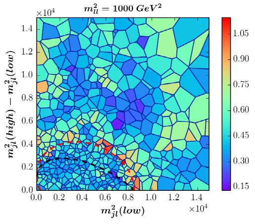
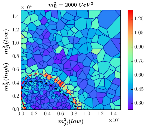
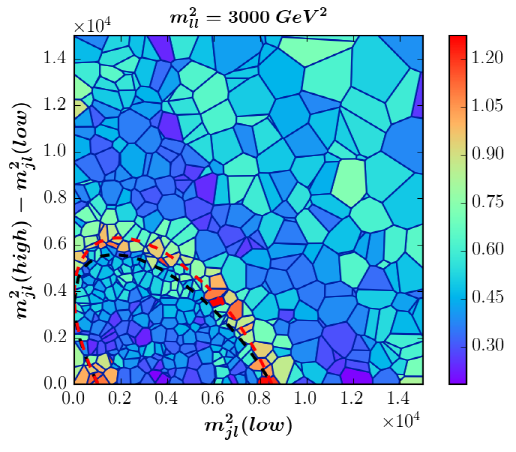
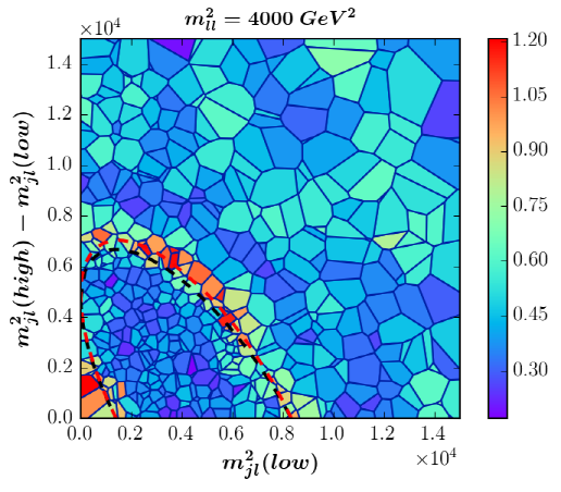
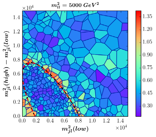
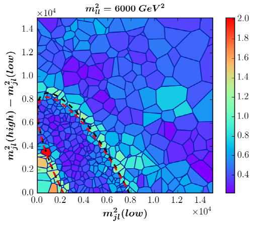
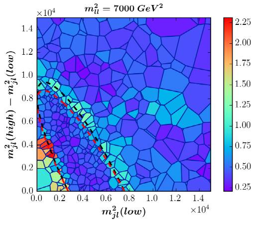
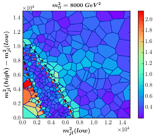
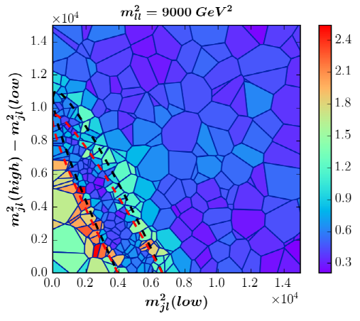
Figure 21: The analogue of Fig. 14 for the physics example considered in section 4.2. We show nine slices at fixed values of $m_{\ell\ell}^{2}$ as indicated at the top of each panel. The red (black) dashed line in each plot corresponds to the expected theoretical boundary implied by eq. (34) for the set of points with $m^{2}_{j\ell_{n}}\geq m^{2}_{j\ell_{f}}$ ($m^{2}_{j\ell_{n}}\leq m^{2}_{j\ell_{f}}$) (see also the third row in Fig. 20).

We are now in position to apply our Voronoi boundary detection algorithm. The result is shown in Fig. 21, where we present nine slices at fixed values of $m_{\ell\ell}^{2}$ as indicated at the top of each panel. The red (black) dashed line in each plot corresponds to the expected theoretical boundary implied by eq. (34) for the set of points with $m^{2}_{j\ell_{n}}\geq m^{2}_{j\ell_{f}}$ ($m^{2}_{j\ell_{n}}\leq m^{2}_{j\ell_{f}}$) (see also the third row in Fig. 20). As before, the signal and background events were normalized so that $\rho=4$. Fig. 21 demonstrates that the Voronoi cells with the highest values of RSD $\bar{\sigma}_{i}$ (colored in red or orange) are indeed found near the theoretical boundaries (the red or black dashed lines). As anticipated, the method performs well for intermediate values of $m^{2}_{\ell\ell}\sim(4,000-5,000)\ {\rm GeV}^{2}$, where the two boundaries resulting from the reordering (38) tend to overlap. We also observe that the boundary closer to the origin also seems to be singled out, especially at high values of $m^{2}_{\ell\ell}$.

5 Conclusions

In this paper, we took the first steps towards developing a general method for identifying surface boundaries in 3D phase space distributions from Voronoi tessellations. In the case of a sequential cascade decay like the one exhibited in Fig. 1, the surface boundary in the relevant $(m_{12},m_{23},m_{13})$ space is characterized by two properties: 1) it is the location of points where the number density is enhanced, due to the $\Delta_{4}^{-1/2}$ factor in the phase space distribution (25) Agrawal:2013uka ; 2) it is the location of points where the number density suddenly changes due to the lack of signal events outside the kinematically allowed boundary. These two properties motivate the use of the geometric variables, $\bar{\sigma}_{i}$ and $\bar{v}_{i}$, derived from the Voronoi tessellation of the data. (For other options, see Debnath:2015wra .) We showed that the edge cells tend to have large values of $\bar{\sigma}_{i}$ and small values of $\bar{v}_{i}$, thus we advocated empirically selected cuts in terms of $\bar{v}_{i}$ and $\bar{\sigma}_{i}$ for tagging edge cell candidates. We considered several examples of increasing complexity and quantified the efficiency of those selection cuts using the language of ROC curves.

There are several directions in which this line of research can proceed from here.

• Statistical significance of a set of tagged edge cells. As we have seen in Figs. 18 and 19, the method is not perfect, in the sense that it occasionally tags a few bulk cells. Therefore, we need to develop a statistical procedure for determining the statistical significance of a given observed set of tagged edge cell candidates. Such a procedure should involve not just the relative number of tagged cells, but also their correlations, e.g., proximity to each other, connectedness, etc. This is an interesting subject on its own and will be addressed in a future publication del4short .

• Parameter measurements from fitting to a set of tagged edge cells. Having selected a set of edge cell candidates, one could imagine fitting to the theoretical prediction for the shape of the boundary surface (34), obtaining a measurement of the mass spectrum of the new particles $X_{1},X_{2},X_{3},X_{4}$. The actual fitting can be done in several different ways, which will also be investigated in del4short .

• Experimental effects. In order to keep the discussion simple and to the point, in this paper we have ignored the experimental complications arising from finite particle widths, detector resolution, ISR jet combinatorics, fakes, etc. Our goal was to present the method as a proof of principle, since the Voronoi approach to data analysis is still in its infancy. Once Voronoi-based methods have become more established and mature, it will become worthwhile to perform detailed and more realistic studies beyond parton level and with full detector simulation.

Here we have focused on cases where the number of signal events on the boundary is significant, leading to a “step” function discontinuity in the total density of events as one moves across the boundary. However, there are interesting examples of distributions where the number density is continuous, but exhibits a “kink”, i.e., a discontinuity in its derivative (gradient)  Han:2009ss ; Han:2012nm ; Han:2012nr . In such cases, our methods can still be applied — not directly on the initial data itself, but on a secondary data sample created by taking suitable derivatives. Indeed, while we have identified and studied a promising use of Voronoi tessellations in the analysis of particle physics data, there are many exciting applications yet to be developed. We look forward with anticipation to the future development and adoption of these novel and powerful methods.

Appendix A ROC Curves and Sensitivity Measures

ROC (receiver operating characteristic) curves are a useful tool for measuring the sensitivity of a variable.

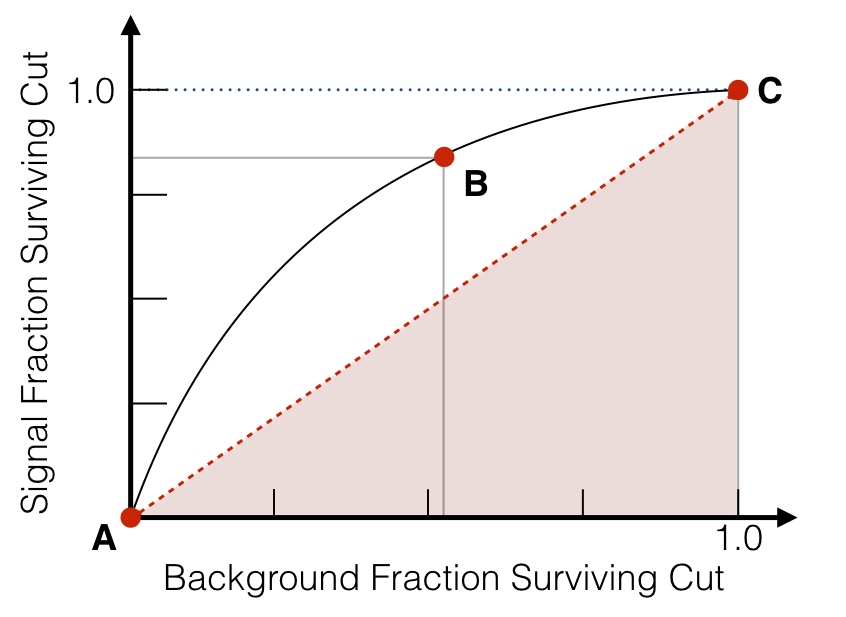
Figure 22: Schematic illustrating the construction of the ROC curve. Each point along the curve indicates the fractions of signal and background events that pass a parameterizable cut. If the cut parameter is chosen to disallow all signal and all background events, we are at the point labelled “A”, while if the cut parameter is chosen to allow signal and background events, then the appropriate point is “C”. An intermediate point, where a certain fraction of signal and background events are allowed is labelled by “B”.

As shown in Fig. 22, the ROC curve is found by (i) defining an event selection procedure (“cut”) based on the variable in question and (ii) determining the fraction, $\varepsilon_{S}$, of signal events, and the fraction, $\varepsilon_{B}$, of background events that pass the given cut. The coordinates of each point along the curve are then provided by $(\epsilon_{B},\epsilon_{S})$. It is easy to see that the ROC curve must include the point $(0,0)$, “A” in Figs. 22 and 23, where all events, signal and background, have been disallowed by the cut. The point $(1,1)$, where all events pass the cut (“C” in Figs. 22 and 23), is also part of every ROC curve. ROC curves have a number of important and useful properties which we shall explore in the remainder of this section.

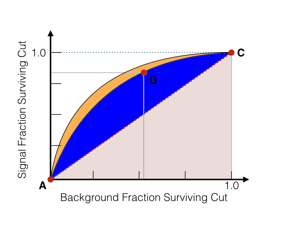
Figure 23: Schematic illustrating the connection between the Gini coefficient (63) and sensitivity. Points “A”, “B”, and “C” from Fig. 22 together with the ROC curve from Fig. 22 are reproduced here. We have also indicated the ROC curve of a perfectly insensitive cut, which is shown by the line from point “A” to point “C”. Finally we have shown a ROC curve for a cut which gives a higher signal fraction for every choice of background fraction than the ROC curve from Fig. 22. We see that the area under the ROC curve of the perfectly insensitive variable (shown in pink) is $1/2$, that there is additional area under the ROC curve shown in Fig. 22 (shown in blue), and that there is even an even greater area under the ROC curve for the more sensitive variable.

A.1 Comparing ROC curves

If we consider two ROC curves, $R_{1}(\varepsilon_{B})$ and $R_{2}(\varepsilon_{B})$, obtained for the same signal and background processes using different choices of variable and/or the cut procedure, then if

$$R_{1}(\varepsilon_{B})\geq R_{2}(\varepsilon_{B})~{}\mathrm{for}~{}\mathrm{all}~{}\varepsilon_{B},$$ (39)

the variable/ cut combination used to produce $R_{1}$ is clearly more sensitive than the variable/cut combination used to produce $R_{2}$. This statement is uncontroversial, but the comparison is not always applicable, as a pair of ROC curves, $R_{1}$ and $R_{2}$ may have points $\varepsilon_{B,1}\neq\varepsilon_{B,2}$ such that

$$R_{1}(\varepsilon_{1})>R_{2}(\varepsilon_{1}),$$ (40)

but

$$R_{1}(\varepsilon_{2})<R_{2}(\varepsilon_{2}).$$ (41)

We will therefore need to develop other procedures to compare ROC curves; we will present several approaches in section A.4. First, however, we must investigate the connection between ROC curves and likelihood and explore some of the more important consequences of this relationship.

A.2 ROC curves and likelihood

There are many ways to perform an analysis using a given variable, and hence many ROC curves that may be constructed with no other information than the value of a given variable for signal and background events. We note that the ratio of signal and background likelihoods is an optimal test statistic, i.e., choosing to accept an event, $e$, when

$$\frac{L_{S}(e)}{L_{B}(e)}\geq l({\varepsilon_{B}}),$$ (42)

where $L_{S}$ is the signal likelihood and $L_{B}$ is the background likelihood, is the procedure which accepts the maximum fraction of signal events ($\varepsilon_{S})$ for a given choice of $\varepsilon_{B}$ (which in turn determines the numerical value of $l(\varepsilon_{B})$ in eq. (42)). This fact is known as the Neyman-Pearson lemma neyman1992problem and is equivalent to the statement that the likelihood ratio produces the optimal ROC curve.

We now provide a heuristic proof of this assertion in terms of ROC curves, which hopefully provides useful insights into both ROC curves and the Neyman-Pearson lemma. We consider the situation where signal and background likelihoods are calculated numerically from samples of signal and background events, $S$ and $B$, which can be assumed arbitrarily large in order to approximate analytic expressions with any desired accuracy. First, we create a set of “variable bins” in our variable of interest, i.e.,

$$V_{i}=[v_{min,i},v_{max,i}),$$ (43)

such that for every event, $e$, in our signal and background samples,

$$v(e)\in[v_{min,i},v_{max,i})$$ (44)

for exactly one choice of $i$, where $v(e)$ refers to the value of the variable under consideration obtained from the event, $e$. We then divide our signal and background events into bins using the values of the variable, $v$, under consideration. I.e., we obtain “signal bins”

$$S_{i}=\{e~{}|~{}v(e)\in V_{i}\}~{}\mathrm{for}~{}e\in S$$ (45)

and “background bins”

$$B_{i}=\{e~{}|~{}v(e)\in V_{i}\}~{}\mathrm{for}~{}e\in B.$$ (46)

Since every signal and every background event must be in some bin, by construction, we have

$$\sum_{i}|S_{i}|=|S|$$ (47)

and

$$\sum_{i}|B_{i}|=|B|.$$ (48)

Hence the estimators of the signal and background likelihood,

$$L_{S,i}=L_{S}(v_{i})\approx|S_{i}|/|S|~{}\mathrm{for}~{}v_{i}\in V_{i}$$ (49)

and

$$L_{B,i}=L_{B}(v_{i})\approx|B_{i}|/|B|~{}\mathrm{for}~{}v_{i}\in V_{i},$$ (50)

are automatically normalized. Further, we note that the contribution to the ROC curve from bin $i$ is a line segment from initial point $(\varepsilon_{B,0},~{}\varepsilon_{S,0})$ to $(\varepsilon_{B,0}+|B_{i}|/|B|,~{}\varepsilon_{S,0}+|S_{i}|/|S|)$, i.e. from $(\varepsilon_{B,0},~{}\varepsilon_{S,0})$ to $(\varepsilon_{B,0}+L_{B,i},~{}\varepsilon_{S,0}+L_{S,i})$. We therefore see from eqs. (49) and (50) that the slope of the line segment corresponding to a particular bin is given by the ratio of signal and background likelihoods calculated for that bin. An interesting corollary, since $L_{S,i}$ and $L_{B,i}$ are always non-negative, is that the ROC curve must be monotonically increasing, i.e.,

$$\frac{d\varepsilon_{S}}{d\varepsilon_{B}}\geq 0.$$ (51)

We now assert that any physically reasonable cut procedure accepts a set of variable bins

$$V_{A}={v\in V_{i}}~{}\mathrm{for}~{}i\in\{i_{1},i_{2},...\},$$ (52)

signal events

$$S_{A}={e\in S_{i}}~{}\mathrm{for}~{}i\in\{i_{1},i_{2},...\},$$ (53)

and background events

$$B_{A}={e\in B_{i}}~{}\mathrm{for}~{}i\in\{i_{1},i_{2},...\},$$ (54)

where $\{i_{1},i_{2},...\}$ are the indices of the variable bins which pass the cut. Further if we have a cut that can be parameterized and that ranges from a cut in which all events are accepted to a cut in which no events are accepted, then we can express the cut function as a permutation, $p$ of $1,2,...,n$, where $n$ is the number of bins, such that the variable bin labelled by $p(1)$ is the last to be eliminated, the variable bin eliminated by $p(2)$ is the next-to-last to be eliminated, etc.

The optimal cut function identified by the Neyman-Pearson lemma, i.e., eq. (42) corresponds to the case where $p(1)$ labels a bin with the maximum value of signal to background likelihood ratio and

$$\frac{L_{S}(v_{p(i)})}{L_{B}(v_{p(i)})}\geq\frac{L_{S}(v_{p(j)})}{L_{B}(v_{p(j)})}$$ (55)

if $i>j$. We claim that this gives the ROC curve for which $\varepsilon_{S}(\varepsilon_{B})$ is maximized for any choice of $\varepsilon_{B}$. This is geometrically obvious given that the likelihood ratio gives the slope of the line segment in the ROC curve; the optimal ROC curve is one in which the steepest segments occur first. A more rigourous proof notes that the ROC curve based on the likelihood ratio has

$$\varepsilon_{S}=\sum_{i}^{m}\frac{L_{S,p(i)}}{L_{B,p(i)}}L_{B,i}+f_{m+1}\frac{L_{S,p(m+1)}}{L_{B,p(m+1)}}L_{B,(m+1)},$$ (56)

where

$$\varepsilon_{B}=\sum_{i}^{m}L_{B,i}+f_{m+1}L_{B,(m+1)}.$$ (57)

and $f_{m+1}\in[0,1]$ is the fraction of bin $m+1$ that must be included to give the desired value of $\varepsilon_{B}$.

We now consider the value of $\varepsilon_{S}$ at the same value of $\varepsilon_{B}$ in a different ROC curve. Since this ROC curve differs from the optimal ROC curve described by eqs. (56-57), it must include some different bins or different fractions of bins. These “new bins” give a contribution to $\varepsilon_{B}$ of $\Delta\varepsilon_{B}$, which is also the contribution to $\varepsilon_{B}$ from the “replcaed original bins” they replace. The contribution to $\varepsilon_{S}$ from the replaced original bins was $\Delta\varepsilon_{S}$, and can be found by multiplying $\Delta\varepsilon_{B}$ by the (appropriately weighted) average slope of the replaced original bins. The contribution to $\varepsilon_{S}$ from the new bins is also the weighed average slope of the bins. However every bin in the new bins has a slope less than or equal to the slope of any bin in the replaced original bins. Thus the value of $\varepsilon_{S}$ in the new ROC curve is less than or equal to its value in the ROC curve based on the likelihood ratio.

A.3 Subdividing variable bins

We now consider the effect on our ROC curve of subdividing a bin, by which we mean that we take a bin, $V_{i}$, and break it into two bins, which we label $V_{i}$ and $V_{n+1}$ as follows:

$$V_{i}=[v_{i,min},v_{i,max})\to[v_{i,min},v_{i^{\prime},max})~{}\mathrm{and}~{}[v_{i^{\prime},max},v_{i,max})=V_{i^{\prime}}~{}\mathrm{and}~{}V_{i^{\prime\prime}}.$$ (58)

We then obtain the signal bins $S_{i}$ and $S_{n+1}$ following eq. (45) and the background bins $B_{i}$ and $B_{n+1}$ following eq. (46). Using these new bins will always allow for the construction of a ROC curve that is as good as or better than the curve before subdivision (in the sense of eq. (39)). This is clear as if the permutation of bins that led to the original ROC curve is $p$, then the permutation

$$p^{\prime}(j)=p(j)~{}\mathrm{for}~{}j<i$$ (59)

$$p^{\prime}(i)=i~{}(\mathrm{which}~{}\mathrm{now}~{}\mathrm{refers}~{}\mathrm{to}~{}\mathrm{a}~{}\mathrm{fraction}~{}\mathrm{of}~{}\mathrm{the}~{}\mathrm{original}~{}\mathrm{bin,}~{}i)$$ (60)

$$p^{\prime}(i+1)=i^{\prime}=n+1$$ (61)

$$p^{\prime}(j)=p(j-1)~{}\mathrm{for}~{}j>i+1$$ (62)

yields a ROC curve which is the same everywhere except in the region corresponding to the subdivided bin. If the two “daughter” bins have the same slope (likelihood ratio), then this curve will be exactly the same as the original ROC curve. However, if this is not the case, then if we choose (without loss of generality) the daughter bin with the greater slope to come first (i.e., to be labelled as $i$), we have a ROC curve which has strictly greater signal values than the original ROC curve in the regime corresponding to the subdivided bin. Finally, it is possible that daughter bin $i$ may have a greater slope than some of the other bins, that daughter bin $n+1$ may have a lesser slope than some of the other bins, or both of these possibilities may be realized. In all of these cases the ROC curve may be further imporoved by sorting the bins by slope.

As a consequence of this result considering smaller bins will increase sensitivity; the extreme limit is to use an unbinned likelihood rather than binned likelihood. While we have not proved it, this fact also motivates the (true) statement that considering additional relevant, but still independent, variables will improve sensitivity (as subdividing a bin using the new variable may yield daughter bins with different slopes).

However, it should be noted, when using actual samples of signal and background events to construct likelihoods, that one can reach false conclusions about sensitivity by subdividing bins too far. An extreme example of this is provided by the case where all the signal and background events we are considering have their own bin. In this case, the likelihood ratio is infinite for bins with one signal event and zero for bins with one background event and the ROC curve is vertical from $(0,0)$ to $(0,1)$, and then horizontal from $(0,1)$ to $(1,1)$. Obviously this is too good to be true. What has happened is an example of posterior statistics and is clearly an invalid inference. Clearly such a situation should be avoided, e.g., by using bins large enough to be robust with respect to statistical fluctuations.

A.4 Measures of ROC curve sensitivity

In section A.1, we noted that sometimes a ROC curve will indicate that one variable/ cut procedure is absolutely better than another variable/ cut procedure. However, this may not always be the case. Thus it is important to have procedures for comparing ROC curves (and hence sensitivity) that always allow the comparison to be made. All of these procedures can be viewed as functionals, i.e., they describe a ROC curve by a number that corresponds directly to the quality of a variable.

Simple functionals that can be used are (i) the value of $\varepsilon_{S}$ at a fixed value of $\varepsilon_{B}$ and (ii) the value of $\varepsilon_{B}$ at a fixed value of $\varepsilon_{S}$. We can view (i) as the fraction of signal events chosen with a fixed false positive rate, while in (ii) we demand that the cut accept a fixed fraction of signal events. A better variable will then reject a larger fraction of background events.

In particle physics, we are generally interested in the significance with which we can claim the discovery (or the exclusion) of some process. Therefore we can describe ROC curves by (i) the maximum value of $S/\sqrt{B}$ attained on the ROC curve, (ii) the maximum value of $S/B$ attained on the ROC curve, or (iii) the maximum discovery significance on the ROC curve. Choice (i) is appropriate as a measure of significance in the (Gaussian) limit of a large number of events in situations where systematic uncertainties do not have a large effect. Choice (ii) is appropriate in the situation where systematic errors dominate. There are different appropaches to implementing choice (iii) to model the statistical and systematic components of the significance. The difference between the Gaussian and Poisson distributions for small numbers of events may also be modelled. While choice (iii) represents the actual quantity to be maximized for a specifc analysis, it has the drawbacks of (i) being complicated and (ii) being dependent on specific experimental conditions, such as the luminosity gathered, systematic uncertainties, etc.

To make comparisons between ROC curves in a general way, we note that the worst possible likelihood-based ROC curve is the ROC curve that reflects throwing away signal and background events indiscriminately, i.e. a straight line from (“A” to “C” in Figs. 22 and 23). On the other hand, a perfect variable would take us from “A” to $(0,1)$ to “C”. This ROC curve contains the entire range of $\varepsilon_{B}$ and $\varepsilon_{S}$ underneath it, suggesting the use of the integral of the ROC curve as a sensitivity measure. Further, as indicated in Fig. 23, variables which lead to “better” ROC curves, in the sense of eq. (39) in section A.1 have more area under their ROC curves. In order for the worst possible likelihood ROC curve to have a value of $0$ and the best possible ROC curve to have a value of $1$, we multiply the integral under the ROC curve by $2$ and subtract $1$. The resulting expression,

$$G_{1}\equiv 2\,{\rm AUROC}-1=2\int_{0}^{1}d\varepsilon_{B}\times\varepsilon_{S}(\varepsilon_{B})-1,$$ (63)

where AUROC referes to the “area under the ROC curve”, e.g., under curve $ABC$ in Figs. 22 and 23 gives the measure of sensitivity known as the Gini coefficient; it is our main quantifier of ROC curves (and hence of variable/ cut procedure sensitivity) in the bulk of this work.

References

- (1) For a basic introduction to Voronoi tessellations, see, e.g., S. Okabe, B. Boots and K. Sugihara, “Spatial Tessellations: Concepts and Applications of Voronoi Diagrams,” John Wiley & Sons, 1992.
- (2) L. Schlicht, M. Valcu and B. Kempenaers, “Thiessen polygons as a model for animal territory estimation,” Ibis 156, no. 1, 215-219 (2014).
- (3) M. Ramella, W. Boschin, D. Fadda and M. Nonino, “Finding galaxy clusters using voronoi tessellations,” Astron. Astrophys. 368, 776 (2001) doi:10.1051/0004-6361:20010071 [astro-ph/0101411].
- (4) M. Cappellari and Y. Copin, “Adaptive spatial binning of integral-field spectroscopic data using voronoi tessellations,” Mon. Not. Roy. Astron. Soc. 342, 345 (2003) doi:10.1046/j.1365-8711.2003.06541.x [astro-ph/0302262].
- (5) L. Giomi and M. Bowick, “Crystalline Order On Riemannian Manifolds With Variable Gaussian Curvature And Boundary,” Phys. Rev. B 76, 054106 (2007) [arXiv:cond-mat/0702471].
- (6) M. Cacciari, G. P. Salam and G. Soyez, “FastJet User Manual,” Eur. Phys. J. C 72, 1896 (2012) doi:10.1140/epjc/s10052-012-1896-2 [arXiv:1111.6097 [hep-ph]].
- (7) B. Abbott et al. [D0 Collaboration], “Search for new physics in data at DØ using Sherlock: A quasi model independent search strategy for new physics,” Phys. Rev. D 62, 092004 (2000) doi:10.1103/PhysRevD.62.092004 [hep-ex/0006011].
- (8) B. Abbott et al. [D0 Collaboration], “A quasi-model-independent search for new high physics at DØ,” Phys. Rev. Lett. 86, 3712 (2001) doi:10.1103/PhysRevLett.86.3712 [hep-ex/0011071].
- (9) T. Aaltonen et al. [CDF Collaboration], “Model-Independent and Quasi-Model-Independent Search for New Physics at CDF,” Phys. Rev. D 78, 012002 (2008) doi:10.1103/PhysRevD.78.012002 [arXiv:0712.1311 [hep-ex]].
- (10) T. Aaltonen et al. [CDF Collaboration], “Global Search for New Physics with 2.0 fb-1 at CDF,” Phys. Rev. D 79, 011101 (2009) doi:10.1103/PhysRevD.79.011101 [arXiv:0809.3781 [hep-ex]].
- (11) D. Debnath, J. S. Gainer, D. Kim and K. T. Matchev, “Edge Detecting New Physics the Voronoi Way,” Europhys. Lett. 114, no. 4, 41001 (2016) doi:10.1209/0295-5075/114/41001 [arXiv:1506.04141 [hep-ph]].
- (12) S. P. Martin, “A Supersymmetry primer,” Adv. Ser. Direct. High Energy Phys. 21, 1 (2010) [Adv. Ser. Direct. High Energy Phys. 18, 1 (1998)] [hep-ph/9709356].
- (13) T. Appelquist, H. C. Cheng and B. A. Dobrescu, “Bounds on universal extra dimensions,” Phys. Rev. D 64, 035002 (2001) doi:10.1103/PhysRevD.64.035002 [hep-ph/0012100].
- (14) H. C. Cheng and I. Low, “TeV symmetry and the little hierarchy problem,” JHEP 0309, 051 (2003) doi:10.1088/1126-6708/2003/09/051 [hep-ph/0308199].
- (15) A. J. Barr and C. G. Lester, “A Review of the Mass Measurement Techniques proposed for the Large Hadron Collider,” J. Phys. G 37, 123001 (2010) doi:10.1088/0954-3899/37/12/123001 [arXiv:1004.2732 [hep-ph]].
- (16) I. Hinchliffe, F. E. Paige, M. D. Shapiro, J. Soderqvist and W. Yao, “Precision SUSY measurements at CERN LHC,” Phys. Rev. D 55, 5520 (1997) doi:10.1103/PhysRevD.55.5520 [hep-ph/9610544].
- (17) H. Bachacou, I. Hinchliffe and F. E. Paige, “Measurements of masses in SUGRA models at CERN LHC,” Phys. Rev. D 62, 015009 (2000) doi:10.1103/PhysRevD.62.015009 [hep-ph/9907518].
- (18) B. C. Allanach, C. G. Lester, M. A. Parker and B. R. Webber, “Measuring sparticle masses in nonuniversal string inspired models at the LHC,” JHEP 0009, 004 (2000) doi:10.1088/1126-6708/2000/09/004 [hep-ph/0007009].
- (19) C. G. Lester, “Model independent sparticle mass measurements at ATLAS,” CERN-THESIS-2004-003.
- (20) B. K. Gjelsten, D. J. Miller and P. Osland, “Measurement of SUSY masses via cascade decays for SPS 1a,” JHEP 0412, 003 (2004) doi:10.1088/1126-6708/2004/12/003 [hep-ph/0410303].
- (21) B. K. Gjelsten, D. J. Miller and P. Osland, “Measurement of the gluino mass via cascade decays for SPS 1a,” JHEP 0506, 015 (2005) doi:10.1088/1126-6708/2005/06/015 [hep-ph/0501033].
- (22) C. G. Lester, M. A. Parker and M. J. White, “Determining SUSY model parameters and masses at the LHC using cross-sections, kinematic edges and other observables,” JHEP 0601, 080 (2006) doi:10.1088/1126-6708/2006/01/080 [hep-ph/0508143].
- (23) D. J. Miller, P. Osland and A. R. Raklev, “Invariant mass distributions in cascade decays,” JHEP 0603, 034 (2006) doi:10.1088/1126-6708/2006/03/034 [hep-ph/0510356].
- (24) C. G. Lester, “Constrained invariant mass distributions in cascade decays: The Shape of the ‘-threshold’ and similar distributions,” Phys. Lett. B 655, 39 (2007) doi:10.1016/j.physletb.2007.08.061 [hep-ph/0603171].
- (25) G. G. Ross and M. Serna, “Mass determination of new states at hadron colliders,” Phys. Lett. B 665, 212 (2008) doi:10.1016/j.physletb.2008.06.003 [arXiv:0712.0943 [hep-ph]].
- (26) A. J. Barr, G. G. Ross and M. Serna, “The Precision Determination of Invisible-Particle Masses at the LHC,” Phys. Rev. D 78, 056006 (2008) doi:10.1103/PhysRevD.78.056006 [arXiv:0806.3224 [hep-ph]].
- (27) A. J. Barr, A. Pinder and M. Serna, “Precision Determination of Invisible-Particle Masses at the CERN LHC. II.,” Phys. Rev. D 79, 074005 (2009) doi:10.1103/PhysRevD.79.074005 [arXiv:0811.2138 [hep-ph]].
- (28) W. S. Cho, D. Kim, K. T. Matchev and M. Park, “Probing Resonance Decays to Two Visible and Multiple Invisible Particles,” Phys. Rev. Lett. 112, no. 21, 211801 (2014) doi:10.1103/PhysRevLett.112.211801 [arXiv:1206.1546 [hep-ph]].
- (29) B. K. Gjelsten, D. J. Miller and P. Osland, “Resolving ambiguities in mass determinations at future colliders,” eConf C 050318, 0211 (2005) [hep-ph/0507232].
- (30) M. Burns, K. T. Matchev and M. Park, “Using kinematic boundary lines for particle mass measurements and disambiguation in SUSY-like events with missing energy,” JHEP 0905, 094 (2009) doi:10.1088/1126-6708/2009/05/094 [arXiv:0903.4371 [hep-ph]].
- (31) K. T. Matchev, F. Moortgat, L. Pape and M. Park, “Precise reconstruction of sparticle masses without ambiguities,” JHEP 0908, 104 (2009) doi:10.1088/1126-6708/2009/08/104 [arXiv:0906.2417 [hep-ph]].
- (32) I. Hinchliffe and F. E. Paige, “Measurements in gauge mediated SUSY breaking models at CERN LHC,” Phys. Rev. D 60, 095002 (1999) doi:10.1103/PhysRevD.60.095002 [hep-ph/9812233].
- (33) M. M. Nojiri, G. Polesello and D. R. Tovey, “Proposal for a new reconstruction technique for SUSY processes at the LHC,” hep-ph/0312317.
- (34) K. Kawagoe, M. M. Nojiri and G. Polesello, “A New SUSY mass reconstruction method at the CERN LHC,” Phys. Rev. D 71, 035008 (2005) doi:10.1103/PhysRevD.71.035008 [hep-ph/0410160].
- (35) H. C. Cheng, J. F. Gunion, Z. Han, G. Marandella and B. McElrath, “Mass determination in SUSY-like events with missing energy,” JHEP 0712, 076 (2007) doi:10.1088/1126-6708/2007/12/076 [arXiv:0707.0030 [hep-ph]].
- (36) M. M. Nojiri and M. Takeuchi, “Study of the top reconstruction in top-partner events at the LHC,” JHEP 0810, 025 (2008) doi:10.1088/1126-6708/2008/10/025 [arXiv:0802.4142 [hep-ph]].
- (37) H. C. Cheng, D. Engelhardt, J. F. Gunion, Z. Han and B. McElrath, “Accurate Mass Determinations in Decay Chains with Missing Energy,” Phys. Rev. Lett. 100, 252001 (2008) doi:10.1103/PhysRevLett.100.252001 [arXiv:0802.4290 [hep-ph]].
- (38) H. C. Cheng, J. F. Gunion, Z. Han and B. McElrath, “Accurate Mass Determinations in Decay Chains with Missing Energy. II,” Phys. Rev. D 80, 035020 (2009) doi:10.1103/PhysRevD.80.035020 [arXiv:0905.1344 [hep-ph]].
- (39) B. Webber, “Mass determination in sequential particle decay chains,” JHEP 0909, 124 (2009) doi:10.1088/1126-6708/2009/09/124 [arXiv:0907.5307 [hep-ph]].
- (40) C. Autermann, B. Mura, C. Sander, H. Schettler and P. Schleper, “Determination of supersymmetric masses using kinematic fits at the LHC,” arXiv:0911.2607 [hep-ph].
- (41) Z. Kang, N. Kersting, S. Kraml, A. R. Raklev and M. J. White, “Neutralino Reconstruction at the LHC from Decay-frame Kinematics,” Eur. Phys. J. C 70, 271 (2010) doi:10.1140/epjc/s10052-010-1477-1 [arXiv:0908.1550 [hep-ph]].
- (42) M. M. Nojiri, K. Sakurai and B. R. Webber, “Reconstructing particle masses from pairs of decay chains,” JHEP 1006, 069 (2010) doi:10.1007/JHEP06(2010)069 [arXiv:1005.2532 [hep-ph]].
- (43) Z. Kang, N. Kersting and M. White, “Mass Estimation without using MET in early LHC data,” arXiv:1007.0382 [hep-ph].
- (44) J. Hubisz and J. Shao, “Mass Measurement in Boosted Decay Chains with Missing Energy,” Phys. Rev. D 84, 035031 (2011) doi:10.1103/PhysRevD.84.035031 [arXiv:1009.1148 [hep-ph]].
- (45) H. C. Cheng, Z. Han, I. W. Kim and L. T. Wang, “Missing Momentum Reconstruction and Spin Measurements at Hadron Colliders,” JHEP 1011, 122 (2010) doi:10.1007/JHEP11(2010)122 [arXiv:1008.0405 [hep-ph]].
- (46) B. Gripaios, K. Sakurai and B. Webber, “Polynomials, Riemann surfaces, and reconstructing missing-energy events,” JHEP 1109, 140 (2011) doi:10.1007/JHEP09(2011)140 [arXiv:1103.3438 [hep-ph]].
- (47) C. G. Lester and D. J. Summers, “Measuring masses of semiinvisibly decaying particles pair produced at hadron colliders,” Phys. Lett. B 463, 99 (1999) doi:10.1016/S0370-2693(99)00945-4 [hep-ph/9906349].
- (48) A. Barr, C. Lester and P. Stephens, “m(T2): The Truth behind the glamour,” J. Phys. G 29, 2343 (2003) doi:10.1088/0954-3899/29/10/304 [hep-ph/0304226].
- (49) M. Baumgart, T. Hartman, C. Kilic and L. T. Wang, “Discovery and measurement of sleptons, binos, and winos with a Z-prime,” JHEP 0711, 084 (2007) doi:10.1088/1126-6708/2007/11/084 [hep-ph/0608172].
- (50) C. Lester and A. Barr, “MTGEN: Mass scale measurements in pair-production at colliders,” JHEP 0712, 102 (2007) doi:10.1088/1126-6708/2007/12/102 [arXiv:0708.1028 [hep-ph]].
- (51) D. R. Tovey, “On measuring the masses of pair-produced semi-invisibly decaying particles at hadron colliders,” JHEP 0804, 034 (2008) doi:10.1088/1126-6708/2008/04/034 [arXiv:0802.2879 [hep-ph]].
- (52) M. Serna, “A Short comparison between and ,” JHEP 0806, 004 (2008) doi:10.1088/1126-6708/2008/06/004 [arXiv:0804.3344 [hep-ph]].
- (53) M. M. Nojiri, K. Sakurai, Y. Shimizu and M. Takeuchi, “Handling jets + missing E(T) channel using inclusive m(T2),” JHEP 0810, 100 (2008) doi:10.1088/1126-6708/2008/10/100 [arXiv:0808.1094 [hep-ph]].
- (54) W. S. Cho, K. Choi, Y. G. Kim and C. B. Park, “M(T2)-assisted on-shell reconstruction of missing momenta and its application to spin measurement at the LHC,” Phys. Rev. D 79, 031701 (2009) doi:10.1103/PhysRevD.79.031701 [arXiv:0810.4853 [hep-ph]].
- (55) H. C. Cheng and Z. Han, “Minimal Kinematic Constraints and m(T2),” JHEP 0812, 063 (2008) doi:10.1088/1126-6708/2008/12/063 [arXiv:0810.5178 [hep-ph]].
- (56) M. Burns, K. Kong, K. T. Matchev and M. Park, “Using Subsystem MT2 for Complete Mass Determinations in Decay Chains with Missing Energy at Hadron Colliders,” JHEP 0903, 143 (2009) doi:10.1088/1126-6708/2009/03/143 [arXiv:0810.5576 [hep-ph]].
- (57) K. Choi, S. Choi, J. S. Lee and C. B. Park, “Reconstructing the Higgs boson in dileptonic W decays at hadron collider,” Phys. Rev. D 80, 073010 (2009) doi:10.1103/PhysRevD.80.073010 [arXiv:0908.0079 [hep-ph]].
- (58) K. T. Matchev and M. Park, “A General method for determining the masses of semi-invisibly decaying particles at hadron colliders,” Phys. Rev. Lett. 107, 061801 (2011) doi:10.1103/PhysRevLett.107.061801 [arXiv:0910.1584 [hep-ph]].
- (59) G. Polesello and D. R. Tovey, “Supersymmetric particle mass measurement with the boost-corrected contransverse mass,” JHEP 1003, 030 (2010) doi:10.1007/JHEP03(2010)030 [arXiv:0910.0174 [hep-ph]].
- (60) P. Konar, K. Kong, K. T. Matchev and M. Park, “Superpartner Mass Measurement Technique using 1D Orthogonal Decompositions of the Cambridge Transverse Mass Variable ,” Phys. Rev. Lett. 105, 051802 (2010) doi:10.1103/PhysRevLett.105.051802 [arXiv:0910.3679 [hep-ph]].
- (61) W. S. Cho, J. E. Kim and J. H. Kim, “Amplification of endpoint structure for new particle mass measurement at the LHC,” Phys. Rev. D 81, 095010 (2010) doi:10.1103/PhysRevD.81.095010 [arXiv:0912.2354 [hep-ph]].
- (62) M. M. Nojiri and K. Sakurai, “Controlling ISR in sparticle mass reconstruction,” Phys. Rev. D 82, 115026 (2010) doi:10.1103/PhysRevD.82.115026 [arXiv:1008.1813 [hep-ph]].
- (63) K. Agashe, R. Franceschini and D. Kim, “Simple ÒinvarianceÓ of two-body decay kinematics,” Phys. Rev. D 88, no. 5, 057701 (2013) doi:10.1103/PhysRevD.88.057701 [arXiv:1209.0772 [hep-ph]].
- (64) K. Agashe, R. Franceschini and D. Kim, “Using Energy Peaks to Measure New Particle Masses,” JHEP 1411, 059 (2014) doi:10.1007/JHEP11(2014)059 [arXiv:1309.4776 [hep-ph]].
- (65) K. Agashe, R. Franceschini, D. Kim and K. Wardlow, “Mass Measurement Using Energy Spectra in Three-body Decays,” JHEP 1605, 138 (2016) doi:10.1007/JHEP05(2016)138 [arXiv:1503.03836 [hep-ph]].
- (66) K. Agashe, R. Franceschini, S. Hong and D. Kim, “Energy spectra of massive two-body decay products and mass measurement,” JHEP 1604, 151 (2016) doi:10.1007/JHEP04(2016)151 [arXiv:1512.02265 [hep-ph]].
- (67) K. Kondo, “Dynamical Likelihood Method for Reconstruction of Events With Missing Momentum. 1: Method and Toy Models,” J. Phys. Soc. Jap. 57, 4126 (1988). doi:10.1143/JPSJ.57.4126
- (68) R. H. Dalitz and G. R. Goldstein, “The Decay and polarization properties of the top quark,” Phys. Rev. D 45, 1531 (1992). doi:10.1103/PhysRevD.45.1531
- (69) V. M. Abazov et al. [D0 Collaboration], “A precision measurement of the mass of the top quark,” Nature 429, 638 (2004) doi:10.1038/nature02589 [hep-ex/0406031].
- (70) J. Alwall, A. Freitas and O. Mattelaer, “Measuring Sparticles with the Matrix Element,” AIP Conf. Proc. 1200, 442 (2010) doi:10.1063/1.3327611 [arXiv:0910.2522 [hep-ph]].
- (71) P. Artoisenet, V. Lemaitre, F. Maltoni and O. Mattelaer, “Automation of the matrix element reweighting method,” JHEP 1012, 068 (2010) doi:10.1007/JHEP12(2010)068 [arXiv:1007.3300 [hep-ph]].
- (72) J. Alwall, A. Freitas and O. Mattelaer, “The Matrix Element Method and QCD Radiation,” Phys. Rev. D 83, 074010 (2011) doi:10.1103/PhysRevD.83.074010 [arXiv:1010.2263 [hep-ph]].
- (73) F. Fiedler, A. Grohsjean, P. Haefner and P. Schieferdecker, “The Matrix Element Method and its Application in Measurements of the Top Quark Mass,” Nucl. Instrum. Meth. A 624, 203 (2010) doi:10.1016/j.nima.2010.09.024 [arXiv:1003.1316 [hep-ex]].
- (74) J. S. Gainer, J. Lykken, K. T. Matchev, S. Mrenna and M. Park, “The Matrix Element Method: Past, Present, and Future,” arXiv:1307.3546 [hep-ph].
- (75) W. S. Cho, K. Choi, Y. G. Kim and C. B. Park, “Gluino Stransverse Mass,” Phys. Rev. Lett. 100, 171801 (2008) doi:10.1103/PhysRevLett.100.171801 [arXiv:0709.0288 [hep-ph]].
- (76) B. Gripaios, “Transverse observables and mass determination at hadron colliders,” JHEP 0802, 053 (2008) doi:10.1088/1126-6708/2008/02/053 [arXiv:0709.2740 [hep-ph]].
- (77) A. J. Barr, B. Gripaios and C. G. Lester, “Weighing Wimps with Kinks at Colliders: Invisible Particle Mass Measurements from Endpoints,” JHEP 0802, 014 (2008) doi:10.1088/1126-6708/2008/02/014 [arXiv:0711.4008 [hep-ph]].
- (78) W. S. Cho, K. Choi, Y. G. Kim and C. B. Park, “Measuring superparticle masses at hadron collider using the transverse mass kink,” JHEP 0802, 035 (2008) doi:10.1088/1126-6708/2008/02/035 [arXiv:0711.4526 [hep-ph]].
- (79) M. M. Nojiri, Y. Shimizu, S. Okada and K. Kawagoe, “Inclusive transverse mass analysis for squark and gluino mass determination,” JHEP 0806, 035 (2008) doi:10.1088/1126-6708/2008/06/035 [arXiv:0802.2412 [hep-ph]].
- (80) A. J. Barr, B. Gripaios and C. G. Lester, “Transverse masses and kinematic constraints: from the boundary to the crease,” JHEP 0911, 096 (2009) doi:10.1088/1126-6708/2009/11/096 [arXiv:0908.3779 [hep-ph]].
- (81) K. T. Matchev, F. Moortgat, L. Pape and M. Park, “Precision sparticle spectroscopy in the inclusive same-sign dilepton channel at LHC,” Phys. Rev. D 82, 077701 (2010) doi:10.1103/PhysRevD.82.077701 [arXiv:0909.4300 [hep-ph]].
- (82) P. Konar, K. Kong, K. T. Matchev and M. Park, “Dark Matter Particle Spectroscopy at the LHC: Generalizing to Asymmetric Event Topologies,” JHEP 1004, 086 (2010) doi:10.1007/JHEP04(2010)086 [arXiv:0911.4126 [hep-ph]].
- (83) P. Konar, K. Kong and K. T. Matchev, “ : A Global inclusive variable for determining the mass scale of new physics in events with missing energy at hadron colliders,” JHEP 0903, 085 (2009) doi:10.1088/1126-6708/2009/03/085 [arXiv:0812.1042 [hep-ph]].
- (84) P. Konar, K. Kong, K. T. Matchev and M. Park, “RECO level and subsystem : Improved global inclusive variables for measuring the new physics mass scale in events at hadron colliders,” JHEP 1106, 041 (2011) doi:10.1007/JHEP06(2011)041 [arXiv:1006.0653 [hep-ph]].
- (85) A. J. Barr, T. J. Khoo, P. Konar, K. Kong, C. G. Lester, K. T. Matchev and M. Park, “Guide to transverse projections and mass-constraining variables,” Phys. Rev. D 84, 095031 (2011) doi:10.1103/PhysRevD.84.095031 [arXiv:1105.2977 [hep-ph]].
- (86) T. Robens, “ resurrected,” JHEP 1202, 051 (2012) doi:10.1007/JHEP02(2012)051 [arXiv:1109.1018 [hep-ph]].
- (87) R. Mahbubani, K. T. Matchev and M. Park, “Re-interpreting the Oxbridge stransverse mass variable MT2 in general cases,” JHEP 1303, 134 (2013) doi:10.1007/JHEP03(2013)134 [arXiv:1212.1720 [hep-ph]].
- (88) Y. Bai, H. C. Cheng, J. Gallicchio and J. Gu, “A Toolkit of the Stop Search via the Chargino Decay,” JHEP 1308, 085 (2013) doi:10.1007/JHEP08(2013)085 [arXiv:1304.3148 [hep-ph]].
- (89) W. S. Cho, J. S. Gainer, D. Kim, K. T. Matchev, F. Moortgat, L. Pape and M. Park, “On-shell constrained variables with applications to mass measurements and topology disambiguation,” JHEP 1408, 070 (2014) doi:10.1007/JHEP08(2014)070 [arXiv:1401.1449 [hep-ph]].
- (90) W. S. Cho, J. S. Gainer, D. Kim, K. T. Matchev, F. Moortgat, L. Pape and M. Park, “Improving the sensitivity of stop searches with on-shell constrained invariant mass variables,” JHEP 1505, 040 (2015) doi:10.1007/JHEP05(2015)040 [arXiv:1411.0664 [hep-ph]].
- (91) W. S. Cho, J. S. Gainer, D. Kim, S. H. Lim, K. T. Matchev, F. Moortgat, L. Pape and M. Park, “OPTIMASS: A Package for the Minimization of Kinematic Mass Functions with Constraints,” JHEP 1601, 026 (2016) doi:10.1007/JHEP01(2016)026 [arXiv:1508.00589 [hep-ph]].
- (92) P. Konar and A. K. Swain, “Mass reconstruction with under constraint in semi-invisible production at a hadron collider,” Phys. Rev. D 93, no. 1, 015021 (2016) doi:10.1103/PhysRevD.93.015021 [arXiv:1509.00298 [hep-ph]].
- (93) P. Agrawal, C. Kilic, C. White and J. H. Yu, “Improved mass measurement using the boundary of many-body phase space,” Phys. Rev. D 89, no. 1, 015021 (2014) doi:10.1103/PhysRevD.89.015021 [arXiv:1308.6560 [hep-ph]].
- (94) D. Costanzo and D. R. Tovey, “Supersymmetric particle mass measurement with invariant mass correlations,” JHEP 0904, 084 (2009) doi:10.1088/1126-6708/2009/04/084 [arXiv:0902.2331 [hep-ph]].
- (95) D. Kim, K. T. Matchev and M. Park, “Using sorted invariant mass variables to evade combinatorial ambiguities in cascade decays,” JHEP 1602, 129 (2016) doi:10.1007/JHEP02(2016)129 [arXiv:1512.02222 [hep-ph]].
- (96) I. W. Kim, “Algebraic Singularity Method for Mass Measurement with Missing Energy,” Phys. Rev. Lett. 104, 081601 (2010) doi:10.1103/PhysRevLett.104.081601 [arXiv:0910.1149 [hep-ph]].
- (97) G. Voronoi, “Nouvelles applications des paramètres continus à la théorie des formes quadratiques,” Journal für die Reine und Angewandte Mathematik, 133, 97 (1908).
- (98) G. L. Dirichlet, “Über die Reduktion der positiven quadratischen Formen mit drei unbestimmten ganzen Zahlen,” Journal für die Reine und Angewandte Mathematik, 40, 209 (1850).
- (99) R. Descartes, Principia philosophiae (1644).
- (100) See, e.g., R. E. Miles and R. J. Maillardet, “The basic structures of Voronoi and generalized Voronoi polygons,” J. of Appl. Prob. 19A, 97-112 (1982).
- (101) J. M. Drouffe and C. Itzykson, “Random Geometry and the Statistics of Two-dimensional Cells,” Nucl. Phys. B 235, 45 (1984). doi:10.1016/0550-3213(84)90147-0
- (102) A. L. Hinde and R. E. Miles, “Monte Carlo estimates of the distributions of the random polygons of the Voronoi tessellation with respect to a Poisson process,” J. Statist. Comput. Simul. 10, 205-223 (1980).
- (103) D. Debnath, J. S. Gainer, D. Kim and K. T. Matchev, “Discovering New Physics with Voronoi Tessellations,” arXiv:1511.02724 [hep-ph].
- (104) U. Lorz, “Distribution of cell characteristics of the spatial Poisson-Voronoi tessellation and plane sections,” Geometrical Problems of Image Processing, Proc. 1991 Georgenthal workshop, ed. U. Eckhardt, A. Hbler, W. Nagel and G. Werner, Akademie-Verlag, 1991, pp. 171-178.
- (105) N. Byers and C. N. Yang, “Physical Regions in Invariant Variables for Particles and the Phase-Space Volume element”, Rev. Mod. Phys. 36, 595 (1964).
- (106) K. A. Olive et al. [Particle Data Group Collaboration], “Review of Particle Physics,” Chin. Phys. C 38, 090001 (2014). doi:10.1088/1674-1137/38/9/090001
- (107) D. Debnath, J. .S. Gainer, C. Kilic, D. Kim, K. T. Matchev, and Y.-P. Yang, in progress.
- (108) J. Alwall, M. Herquet, F. Maltoni, O. Mattelaer and T. Stelzer, “MadGraph 5 : Going Beyond,” JHEP 1106, 128 (2011) doi:10.1007/JHEP06(2011)128 [arXiv:1106.0522 [hep-ph]].
- (109) G. Aad et al. [ATLAS Collaboration], “Search for supersymmetry in events containing a same-flavour opposite-sign dilepton pair, jets, and large missing transverse momentum in TeV pp collisions with the ATLAS detector,” Eur. Phys. J. C 75, no. 7, 318 (2015) Erratum: [Eur. Phys. J. C 75, no. 10, 463 (2015)] doi:10.1140/epjc/s10052-015-3661-9, 10.1140/epjc/s10052-015-3518-2 [arXiv:1503.03290 [hep-ex]].
- (110) T. Han, I. W. Kim and J. Song, “Kinematic Cusps: Determining the Missing Particle Mass at Colliders,” Phys. Lett. B 693, 575 (2010) doi:10.1016/j.physletb.2010.09.010 [arXiv:0906.5009 [hep-ph]].
- (111) T. Han, I. W. Kim and J. Song, “Kinematic Cusps With Two Missing Particles I: Antler Decay Topology,” Phys. Rev. D 87, no. 3, 035003 (2013) doi:10.1103/PhysRevD.87.035003 [arXiv:1206.5633 [hep-ph]].
- (112) T. Han, I. W. Kim and J. Song, “Kinematic Cusps with Two Missing Particles II: Cascade Decay Topology,” Phys. Rev. D 87, no. 3, 035004 (2013) doi:10.1103/PhysRevD.87.035004 [arXiv:1206.5641 [hep-ph]].
-
(113)
“Receiver operating characteristic”,
https://en.wikipedia.org/wiki/Receiver_operating_characteristic. Accessed June 8, 2016. - (114) J. Neyman and E. S. Pearson, “On the problem of the most efficient tests of statistical hypotheses”, Philosophical Transactions of the Royal Society of London. Series A, Vol. 231 (1933), pp. 289-337.