Resonant dynamics in higher dimensional anti-de Sitter spacetime

Abstract

We present results from a detailed study of spherically symmetric Einstein-massless-scalar field dynamics with a negative cosmological constant in four to nine spacetime dimensions. This study is the first to present a detailed examination of the dynamics in AdS beyond five dimensions, including a detailed comparison with numerical solutions of perturbative methods and their gauge dependence. Using these perturbative methods, we provide evidence that the oscillatory divergence of the first derivative used to argue for instability of anti-de Sitter space by Bizoń et al. is a gauge-dependent effect in five spacetime dimensions but the divergence of the second derivative is gauge-independent. We find that the divergence of the first derivative appears to be gauge-independent in higher dimensions; however, understanding how this divergence depends on the initial data is more difficult. We also find that four dimensions is more difficult to study than higher dimensions. The results we present show that while much progress has been made in understanding the rich dynamics and stability of anti-de Sitter space, much work is still to be done. The recent work of Moschidis is encouraging that it is possible to understand the problem analytically.

I Introduction

Stability of de Sitter and Minkowski spacetimes under small perturbations was established in 1986Friedrich (1986) and 1993Christodoulou and Klainerman (2014). Following the Anti-de Sitter (AdS)/Conformal Field Theory (CFT) conjectureMaldacena (1999), the question of the stability of AdS became more interesting. Using the AdS/CFT conjecture it is possible to address the important question of thermalization and equilibration of strongly coupled CFTs, which is dual to the question of whether or not small perturbations of AdS collapse to a black hole. The stability of AdS against arbitrarily small scalar field perturbations was first studied numerically in spherical symmetry by Bizoń and Rostworowski in 2011Bizoń and Rostworowski (2011), where the authors suggested that a large class of perturbations eventually collapse to form a black hole even at arbitrarily small amplitude, $\epsilon$. However, in such simulations a finite $\epsilon$ must be used, leaving room for doubt as to whether arbitrarily small perturbations do actually form a black holeDimitrakopoulos et al. (2015). The probing of small-amplitude perturbations is aided by the recently proposed renormalization flow equations (RFEs)Balasubramanian et al. (2014); Craps et al. (2014, 2015a) for which any behavior observed at amplitude $\epsilon$ and time $t/\epsilon^{2}$ is also present at an amplitude $\epsilon^{\prime}$ and time $t/\epsilon^{\prime 2}$. This rescaling symmetry was used by Bizoń et al. to argue for the instability of AdS₅ based on a divergence in the RFE solution for specific initial dataBizoń et al. (2015). However, it is suspected that this divergence is a gauge-dependent effectCraps et al. (2015b). The gauge dependence is understood as an infinite redshift in AdS₅ and signals that the assumption that the system is weakly gravitating is no longer validDimitrakopoulos et al. (2016). Recently, Moschidis has shown that the Einstein–null dust system with an inner mirrorMoschidis (2017) and the Einstein–massless Vlasov systemMoschidis (2018) are unstable.

In this paper, we address the AdS stability question and the concerns of Craps et al. (2015b) by performing a detailed study of the RFEs and the nonlinear Einstein equations. Our study is the first to examine the gauge dependence of the RFEs and dynamics in AdS beyond five dimensions. Our numerical methods enable us to study the RFEs to a much higher accuracy than previous work, providing new insight into when the RFEs are no longer valid and the reasons they fail. With a new understanding of the RFEs we revisit AdS₄, finding agreement with previous workBalasubramanian et al. (2014); Green et al. (2015) but strong contrast with what is observed in higher dimensions. Finally, we show that our results are largely robust against the choice of initial data and present evidence that the dynamics of AdS₄ are more intricate than in higher dimensions.

II Model

We consider a self-gravitating massless scalar field in a spherically symmetric, asymptotically AdS spacetime in $d$ spatial dimensions. The metric in Schwarzschild-like coordinates is

$$ds^{2}=\frac{\ell^{2}\left[-Ae^{-2\delta}dt^{2}+A^{-1}dx^{2}+\sin^{2}\left(\frac{x}{\ell}\right)d\Omega^{d-1}\right]}{\cos^{2}\left(\frac{x}{\ell}\right)},$$ (1)

where $d\Omega^{d-1}$ is the metric on $\mathbb{S}^{d-1}$, $x/\ell\in[0,\pi/2]$, and $t/\ell\in[0,\infty)$. The areal radius is $R(x)=\ell\tan(x/\ell)$, and we henceforth work in units of the AdS scale $\ell$ (i.e. $\ell=1$).

The evolution of the scalar field $\psi$ is governed by the nonlinear system

$$\Phi_{,t}=\left(Ae^{-\delta}\Pi\right)_{,x},\quad\Pi_{,t}=\frac{(Ae^{-\delta}\tan^{d-1}x\Phi)_{,x}}{\tan^{d-1}x},$$ (2)

where $\Pi=A^{-1}e^{\delta}\psi_{,t}$ is the conjugate momentum and $\Phi=\psi_{,x}$ is an auxiliary variable. The metric functions are solved for from

$$\delta_{,x}= -\sin x\cos x(\Pi^{2}+\Phi^{2})$$ (3)

$$A_{,x}= \frac{d-2+2\sin^{2}x}{\sin x\cos x}(1-A)-\sin x\cos x(\Phi^{2}+\Pi^{2}).$$ (4)

See Deppe et al. (2015); Deppe and Frey (2015) for a detailed discussion of the code we use to solve this system. At the origin we choose $A(x=0,t)=1$. Two common gauge choices are the interior time gauge (ITG), where $\delta(x=0,t)=0$, and the boundary time gauge (BTG), where $\delta(x=\pi/2,t)=0$. We perform evolutions of the full nonlinear theory in the ITG.

We are particularly interested in perturbations about AdS_(d+1) whose evolution at linear order is governed by $\hat{L}=-(\tan^{1-d}x)\partial_{x}(\tan^{d-1}x\partial_{x})$ (this can be seen by setting $A=1,$ $\delta=0$ and $\Pi=\psi_{,t}$ in Eq. (2)). The eigenmodes of $\hat{L}$ are given in terms of Jacobi polynomials,

$$e_{j}(x) =\kappa_{j}\cos^{d}(x)P^{(d/2-1,d/2)}_{j}(\cos 2x)$$ (5)

with eigenvalues $\omega_{j}=d+2j$ and where $\kappa_{j}=2\sqrt{j!(j+d-1)!}/\Gamma(j+d/2)$Craps et al. (2015a).

Recently much attention has been given to the renormalization flow or two-time framework equationsBalasubramanian et al. (2014); Craps et al. (2014, 2015a, 2015b); Bizoń et al. (2015); Green et al. (2015). A detailed study of AdS₄ was presented in Green et al. (2015), while Bizoń et al. (2015) investigated AdS₅. To study the RFEs, a “slow time” $\tau=\epsilon^{2}t$ is introduced, and dynamics on very short time scales can be thought of as being averaged over. The scalar field perturbation is expanded as $\psi(x,t)=\sum_{l=0}^{\infty}A_{l}\cos(\omega_{l}t+B_{l})e_{l}(x)$, where $A_{l}(\tau)$ and $B_{l}(\tau)$ are time-dependent coefficients. The evolution of $A_{l}$ and $B_{l}$ is given by the RFEsCraps et al. (2015a)

$$-\frac{dA_{l}}{d\tau}= \sum_{\begin{subarray}{c}i,j,k\\ i+j=k+l\\ \{i,j\}\neq\{k,l\}\end{subarray}}\frac{S_{ijkl}}{2\omega_{l}}A_{i}A_{j}A_{k}\sin(B_{l}+B_{k}-B_{i}-B_{j}),$$ (6)

$$-\frac{dB_{l}}{d\tau}= \sum_{\begin{subarray}{c}i,j,k\\ i+j=k+l\\ \{i,j\}\neq\{k,l\}\end{subarray}}\frac{S_{ijkl}}{2\omega_{l}A_{l}}A_{i}A_{j}A_{k}\cos(B_{l}+B_{k}-B_{i}-B_{j})$$

$$+\frac{T_{l}}{2\omega_{l}}A_{l}^{2}+\sum_{\begin{subarray}{c}i\\ i\neq l\end{subarray}}\frac{R_{il}}{2\omega_{l}}A_{i}^{2},$$ (7)

where $\{i,j\}\neq\{k,l\}$ means both $i$ and $j$ are not equal to $k$ or $l$, and the coefficients $T_{l}$, $R_{il}$ and $S_{ijkl}$ are given by integrals over the eigenmodes in appendix A of Craps et al. (2015a) and by recursion relations in Craps et al. (2015b). The gauge dependence of the coefficients is discussed in Craps et al. (2015b).

In our numerical computations we typically truncate the RFEs (6-II) at $l_{\text{max}}=399$, giving a good balance between computational cost and accuracy, and refer to this system as the truncated RFEs (TRFEs). We note that the evolutions dominate the computational cost, not the construction of $T_{l},R_{il}$ and $S_{ijkl}$, which we have computed to $l_{\rm{max}}>700$. We compute the coefficients $T_{l},R_{il}$ and $S_{ijkl}$ directly by combining the integrals in Craps et al. (2015a) analytically. For the evaluation we have tested Simpson’s rule on a uniform grid and found this to be computationally inefficient. Ultimately we used adaptive Gaussian quadrature with a relative error tolerance of $10^{-10}$.

We tested several algorithms for time integration, including the fifth and eighth order methods by Dormand and Prince, the semi-implicit extrapolation method, and a fully implicit variable order (orders 5, 9 and 13) Gauss-Radau method similar to what is used in Green et al. (2015); Bizoń et al. (2015). We find that choosing good values for the absolute and relative truncation error is important since the $A_{l}$’s decay exponentially and we are interested in their behavior even early on when they are still small. For our simulations we are able to conserve the RFE energy, $E=\sum_{l=0}^{l_{\max}}\omega_{l}{}^{2}|A_{l}|^{2}/4$ to approximately thirteen significant figures and we also see excellent agreement with numerical evolutions of the nonlinear Einstein equations. The results presented here used the eighth order Dormand and Prince method.

III Results

We present results from a detailed study of the TRFEs and full nonlinear numerical evolutions in four to nine spacetime dimensions. For concreteness we focus on two-mode initial data of the form

$$\psi(x,0)=\epsilon(e_{0}(x)+\kappa e_{1}(x))/d$$ (8)

but have also studied Gaussian initial data given by

$$\Pi(x,0)=\epsilon\exp\left(-\frac{\tan^{2}(x)}{\sigma^{2}}\right),\;\;\psi(x,0)=0.\$$ (9)

In the evolutions presented here we choose $\kappa=d/(d+2)$, which has been studied extensively in AdS₄Balasubramanian et al. (2014); Green et al. (2015); Deppe and Frey (2015) and in AdS₅Bizoń et al. (2015) using the ITG. A logarithmic divergence in the time derivative of the phases, $dB_{l}/d\tau$, was observed in Bizoń et al. (2015). This is consistent with an asymptotic analysis of the equations in the ITG; however, the terms leading to the logarithmic divergence appear to be absent in the BTGCraps et al. (2015b). We will address this in detail below.

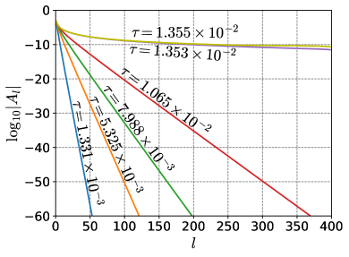
Figure 1: The spectrum $A_{l}$ with $l_{\text{max}}=399$ for initial data (8) in AdS₉ using the ITG. The spectrum becomes singular when $\tau_{\star}=\epsilon^{2}t_{\star}\approx 1.353\times 10^{-2}$.

An interesting technique for analyzing solutions to the TRFEs is the analyticity-strip methodSulem et al. (1983); Bizoń et al. (2015). This method involves fitting the spectrum $A_{l}$ to

$$A_{l}=C(\tau)l^{-\gamma(\tau)}e^{-\rho(\tau)l}$$ (10)

for $l\gg 1$. The analyticity radius $\rho(\tau)$ should be interpreted as the distance between the real axis and the nearest singularity in the complex plane. When $\rho$ becomes zero the TRFEs have evolved to a singular spectrum. We denote the time when the spectrum becomes singular by $\tau_{\star}$(or $t_{\star}=\tau_{\star}/\epsilon^{2}$) and in $d>3$ stop our evolutions of the TRFEs when $\tau$ is slightly larger than $\tau_{\star}$. All fits unless otherwise specified use data from simulations done with $l_{\text{max}}=399$ and omit the lowest and highest twenty modes to reduce errors from truncation. For concreteness we present results in AdS₉ but observe qualitatively identical behavior for $d>3$. The spectrum for initial data (8) in AdS₉ at different times is shown in Fig. 1. At $\tau=1.355\times 10^{-2}$ the spectrum is already singular, so we show it only for completeness.

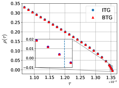
Figure 2: $\rho(\tau)$ for the $l_{\text{max}}=399$ AdS₉ evolution in the ITG and BTG. In both gauges the spectrum becomes singular at $\tau_{\star}\approx 1.353\times 10^{-2}$, suggesting this behavior is gauge-independent.

In Fig. 2 we plot $\rho(\tau)$ for both the ITG and BTG for AdS₉. We observe that the spectrum becomes singular at approximately the same $\tau_{\star}$ in both the BTG and the ITG, independent of the dimension being studied, suggesting this behavior is gauge-independent. Interestingly, in our study of $d>3$ we find that the spectrum becomes singular at approximately the same time that a black hole forms in the full nonlinear theory, at least for the initial data studied. We will discuss this further in the context of AdS₄ below. Note that the TRFEs should no longer be trusted when $\rho\leq 1/l_{\mathrm{max}}$.

Looking at the asymptotic behavior of the $T,R,S$ coefficients for $d>3$ in the ITG we see that $S_{\lambda i,\lambda j,\lambda k,\lambda l}\sim\lambda^{d}S_{ijkl}$, $T_{l}\sim l^{d+1}$, and $R_{il}\sim l^{2}i^{d-1}$Craps et al. (2015b). Substituting $T_{l}$, $R_{jl}$, and Eq. (10) into Eq. (II) we get

$$-2\omega_{l}\frac{dB_{l}}{d\tau}\sim l^{d+1-2\gamma}e^{-2\rho(\tau_{\star}-\tau)l}$$

$$+l^{2}\sum_{\begin{subarray}{c}i\\ i\neq l\end{subarray}}i^{d-1-2\gamma}e^{-2\rho(\tau_{\star}-\tau)i}.$$ (11)

Since $\rho\to 0$ as $\tau\to\tau_{\star}$ the first term goes to a constant as $\tau\to\tau_{\star}$. The sum in the second term evaluates to a polylogarithm,

$$\mathrm{Li}_{2\gamma+1-d}(e^{-2\rho(\tau_{\star}-\tau)}).$$ (12)

In AdS₅ $\gamma=2$ and we get the results of Bizoń et al. (2015) that

$$\frac{dB_{l}}{d\tau}\sim\ln(\tau_{\star}-\tau).$$ (13)

In the BTG the dominant terms in the coefficients go as $S_{\lambda i,\lambda j,\lambda k,\lambda l}\sim\lambda^{d}S_{ijkl}$, $T_{l}\sim l^{d}$, and $R_{il}\sim l^{2}i^{d-2}$. We have verified this by fitting some of the $R_{il}$ coefficients with $l_{\max}=4100$. Substituting into Eq. (II) we see that Eq. (12) describes the second derivative of the phases in the BTG while the first derivative goes as

$$-2\omega_{l}\frac{dB_{l}}{d\tau}\sim l^{d-2\gamma}e^{-2\rho(\tau_{\star}-\tau)l}$$

$$+l^{2}\sum_{\begin{subarray}{c}i\\ i\neq l\end{subarray}}i^{d-2-2\gamma}e^{-2\rho(\tau_{\star}-\tau)i}$$ (14)

$$\sim \mathrm{Li}_{2\gamma+2-d}(e^{-2\rho(\tau_{\star}-\tau)}).$$ (15)

In AdS₅ the asymptotic behavior means that the logarithmic divergence is present in the second time derivative in the BTG, but the first time derivative of the phases remains regular. The presence of the oscillatory singularity in the ITG but not in the BTG in AdS₅ can be understood as the assumption that the system is weakly gravitating is breaking downDimitrakopoulos et al. (2016). Specifically, the redshift becomes infinite and so gravity is no longer weak. The oscillatory blowup is related to this infinite redshift in AdS₅, but its nature is not yet understood in higher dimensionsDimitrakopoulos et al. (2016). However, the redshift in higher dimensions does explain why blowup in the time derivative of the phases occurs at different rates in the ITG and BTG.

$d$	Gauge	$\epsilon$	$\gamma$	$\tilde{\gamma}$	$\tau_{\star}$
4	ITG	0.0317	2	2.07	0.514
4	BTG	0.0317	2	2.11	0.514
8	ITG	0.00516	4	3.84	0.01354
8	BTG	0.00516	4	3.54	0.01354

Table 1: The estimated values of $\gamma$ and $\tau_{\star}$ in AdS₅ and AdS₉. We obtain $\gamma$ by fitting Eq. (10) at $\tau_{\star}$, and also from fitting Eq. (12) and Eq. (15). The value we obtain from Eq. 12 and Eq. 15 we denote by $\tilde{\gamma}$. In the BTG in AdS₅ we fit to $d^{2}B_{l}/d\tau^{2}$ instead of $dB_{l}/d\tau$.

Because determining $\gamma$ from the analyticity-strip method is notoriously difficult we also fit for $\gamma$ keeping $\tau_{\star}$ fixed, since the time when the spectrum becomes singular is estimated more robustly from the analyticity radius. In table 1 we show results of the fits in AdS₅ and AdS₉ in the ITG and BTG, denoting the result of the fit to Eq. (12) in the ITG and Eq. (15) in the BTG by $\tilde{\gamma}$. We note that in the BTG in AdS₅ we fit Eq. (12) to $d^{2}B_{l}/d\tau^{2}$. Because of the difficulty of the fit we only draw the qualitative conclusion that in $d>3$ spatial dimensions the time derivative of the phases blows up at some finite $\tau_{\star}$ that corresponds to black hole formation in the full nonlinear theory, at least in the cases we have studied. In general the blowup is polylogarithmic, is more severe in higher dimensions, and is more severe in the ITG than in the BTG. As suggested in Craps et al. (2015b), there is no logarithmic blowup in $dB_{l}/d\tau$. However, there is a logarithmic blowup in $d^{2}B_{l}/d\tau^{2}$, and since the first integral of $\ln(x)$ does not diverge as $x\to 0$, $dB_{l}/d\tau$ does not diverge in the BTG. This is consistent with an asymptotic analysis of the coefficients. In the top panel of Fig. 3 we show $dB_{l}/d\tau$ in the ITG and $d^{2}B_{l}/d\tau^{2}$ in the BTG along with logarithmic fits to the data in AdS₅, while in the bottom panel we show $dB_{l}/d\tau$ in the ITG and BTG in AdS₉. We analyze the $l=250$ mode because it is far below $l_{\max}$ to minimize errors that stem from mode truncation.

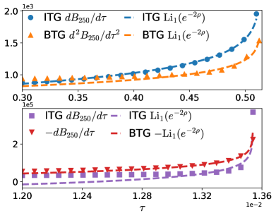
Figure 3: Derivatives of the phase $B_{250}$ in both the ITG and BTG in AdS₅ (top panel) and AdS₉ (bottom panel). We show the second derivative of $B_{l}$ in AdS₅ in the BTG because the first derivative does not exhibit any blowup, as suggested in Craps et al. (2015b). To assess the behavior we fit $\mathrm{Li}_{2\gamma+1-d}(e^{-2\rho(\tau_{\star}-\tau)})$ (dashed lines) to the data. Note that in the BTG in AdS₅ we rescale the second derivative by $1/70$ so that the scales of the first and second derivative are comparable.

In spatial dimensions $d>3$ we observe a direct cascade of energy to higher modes without any inverse cascades, suggesting the initial data is far from a quasi-periodic solutionGreen et al. (2015). In Fig. 4 we show the upper envelope of $\Pi^{2}(x=0,t)/\epsilon^{2}$, which is proportional to the Ricci scalar at the origin, for several different values of $l_{\text{max}}$ and different values of $\epsilon$ for full nonlinear evolutions in AdS₉. There is good agreement between the fully nonlinear and TRFE solutions and the agreement improves with increasing dimensionality, at least for $\Pi^{2}(x=0,t)/\epsilon^{2}$. Because $\Pi(x,t)/\epsilon=\sum_{l=0}^{l_{\mathrm{max}}}\partial_{t}(A_{l}\cos(\omega_{l}t+B_{l}))e_{l}(x=0)/\epsilon$ the improved agreement may be related to the eigenmodes having larger values at $x=0$ in higher dimensions. In Fig. 5 we plot $K_{l}=\partial_{t}(A_{l}\cos(\omega_{l}t+B_{l}))e_{l}(x=0)/\epsilon$ in the ITG for $l=96$ in AdS₅ and AdS₉. We plot $K_{l}$ as a function of $t$ instead of $\tau$ so the two simulations are more readily compared. Near the end of the simulation $K_{l}$ becomes several orders of magnitude larger in AdS₉ than AdS₅. We found qualitatively similar behavior for other values of $l$ and also in the BTG. However, in the BTG the difference between $K_{l}$ in AdS₅ and AdS₉ is smaller by approximately two orders of magnitude than in the ITG. The difference in $K_{l}$ between AdS₅ and AdS₉ arises mostly from $e_{l}(x=0)$. For example, we find that in AdS₉ $e_{250}(x=0)$ is $\sim 10^{4}$ times larger than in AdS₅.

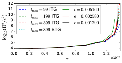
Figure 4: The upper envelope of $\Pi^{2}(x=0,t)$ for two-mode equal-energy data, Eq.  (8), for evolutions in AdS₉. Plotted are solutions to the TRFEs in the ITG (dash lines) and the BTG (dashed-dotted lines) for several different values of $l_{\text{max}}$, and full nonlinear evolutions for $\epsilon=0.00516,0.00258,0.00129$ (solid lines). As expected, the difference between the TRFE and fully nonlinear solution decreases for smaller $\epsilon$ and larger $l_{\rm{max}}$.

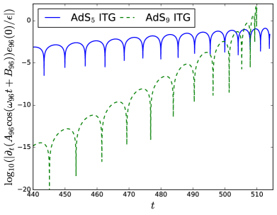
Figure 5: Plot showing how a single term in the series $\Pi(x=0,t)=\sum_{l=0}^{l_{\mathrm{max}}}\partial_{t}(A_{l}\cos(\omega_{l}t+B_{l}))e_{l}(x=0)$ evolves in the ITG comparing AdS₅ and AdS₉ for $l=96$. Similarly behavior is observed for other large $l$ modes and also in the BTG.

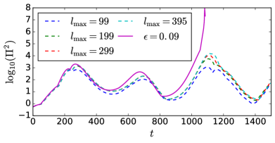
Figure 6: The upper envelope of $\Pi^{2}(x=0,t)$ for two-mode data (8) for evolutions in AdS₄. Plotted are solutions to the TRFEs (dash lines) for different values of $l_{\text{max}}$, and the fully nonlinear evolution (solid line) both using the ITG. The TRFE solutions with $l_{\text{max}}=299$ and $395$ differ only marginally until the third increase in $\Pi^{2}$.

We now turn to the case of two-mode equal-energy data, Eq. (8), in AdS₄. This case has been studied extensively using numerical relativity and the TRFEsBizoń and Rostworowski (2011); Balasubramanian et al. (2014); Bizoń and Rostworowski (2015); Balasubramanian et al. (2015); Deppe and Frey (2015). It was suggested in Green et al. (2015) that this solution orbits a quasi-periodic solution of the same temperature. For these evolutions we use $l_{\text{max}}=99,199,299,$ and 395 to test convergence and to understand how the analyticity radius depends on mode truncation. We compare $\Pi^{2}(x=0,t)$ with the full nonlinear evolution in Fig. 6. The 299 and 395 mode evolutions are almost indistinguishable until the third increase in $\Pi^{2}$. This suggests that the agreement between the TRFE and full nonlinear solutions would improve if a lower amplitude fully nonlinear evolution were studied, similar to what is observed in Fig. 4 for AdS₉. Unfortunately, such an evolution requires a prohibitive amount of computational resources. For concreteness we present results using the ITG but found the same behavior in the BTG. Because of the computational expense of using $l_{\mathrm{max}}=395$ we only studied $l_{\mathrm{max}}=99,199,$ and 299 in the BTG.

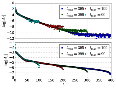
Figure 7: Spectrum of two-mode initial data in AdS₄ using the ITG and various $l_{\mathrm{max}}$ at $t=1000$ (upper panel) and $t=1100$ (lower panel). Mode truncation effects are very apparent at $t=1000$. However, the spectrum is better behaved at later times ($t=1100$). Qualitatively similar behavior is seen at earlier increases in $\Pi^{2}$ as well.

To better understand the reliability of the TRFEs for the two-mode data in AdS₄ we show the spectrum at two different times $t=1000$ (upper panel) and $t=1100$ (lower panel) of Fig. 7. To gain an understanding of mode truncation errors and convergence we compare results using several different values of $l_{\mathrm{max}}$. What we observe is that at $t=1000$ the highest (in $l$) modes are not well-behaved and that this effect is dependent on $l_{\mathrm{max}}$, while lower $l$ modes decay exponentially. Surprisingly, the spectrum using different $l_{\mathrm{max}}$ resemble each other closely again at $t=1100$. We note that the large $l$ modes are similarly poorly behaved after the first two increases in $\Pi^{2}$ in Fig. 6. What may be surprising is that even with the mode truncation effects, $\Pi^{2}$ computed from the TRFEs follows the general trend of the fully nonlinear evolution quite well.

Because of the agreement in $\Pi^{2}$ between the TRFE and fully nonlinear solutions it may be tempting to speculate that the two-mode data in AdS₄ is stable and that the theorems of Dimitrakopoulos and Yang (2015) for behavior of stable solutions should be applied for all times. We believe that this would be premature in light of our new understanding of when the perturbation theory suffers from mode truncation. Given the evidence we have presented for when our results are suffering from mode truncation and the general agreement between $\Pi^{2}$ in the fully nonlinear theory and from the TRFEs, the theorems of Dimitrakopoulos and Yang (2015) suggest that small amplitude equal-energy two-mode initial data is stable at least until $t\approx 1085$ for $\epsilon=0.09$ ($\tau\approx 8.8$). However, we are unable to make predictions about later time behavior.

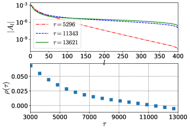
Figure 8: Evolution of Guassian initial data (9) in AdS₄. The spectrum is plotted at several times in the upper panel. In the bottom panel we plot $\rho(\tau)$ in the ITG fitting Eq. (10) to the interval $l\in[25,199]$.

Finally, to understand the genericity of our results we also studied initial data given by Eq. (9). Fully nonlinear evolutions of this data have been well-studied and found to collapseBizoń and Rostworowski (2011); Jałmużna et al. (2011); Buchel et al. (2012, 2013); Deppe and Frey (2015). We find that the TRFEs require a larger $l_{\mathrm{max}}$ for Gaussian data than for the two-mode data to achieve the same accuracy in the sense of how well $\Pi^{2}(x=0)$ is approximated. Nevertheless, for $d>3$ we find similar results as for the two-mode data discussed above.

In the bottom panel of Fig. 8 we plot $\rho(\tau)$, and in the upper panel we plot $|A_{l}|$. While testing how $\rho$ depends on the interval to which Eq. (10) is fit we found that if too many high modes are included then $\rho$ no longer crosses zero, even though a black hole forms in the full nonlinear theory. While a black hole forming in the full nonlinear theory does not mean $\rho$ crosses zero, given the sensitivity to the number of modes to which the fit is done we conclude that in AdS₄ many more modes are needed to accurately follow the dynamics than in higher dimensions.

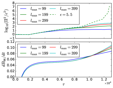
Figure 9: Results from an evolution of Gaussian initial data (9) in AdS₄. The upper panel shows the upper envelope of $\log_{10}(\Pi^{2}/\epsilon^{2})$ at the origin in the ITG with qualitatively identical results in the BTG. The lower panel shows $dB_{96}/dt$ in the ITG with similar results for other modes. In the BTG $dB_{l}/dt$ decreases rather than increases with increasing $\tau$ but similarly illustrates that $l_{\mathrm{max}}=399$ is insufficient to fully captured the large $l$ behavior.

In the upper panel of Fig. 9 we plot $\Pi^{2}/\epsilon^{2}$ showing that $l_{\mathrm{max}}=399$ does not capture the behavior nearly as well as it does for two-mode data and in higher dimensions (compare to Fig. 4). We plot $dB_{96}/dt$ for $l_{\mathrm{max}}=99,199,299$ and 399 in the lower panel of Fig. 9. In agreement with Green et al. (2015), we do not observe a divergence in $dB_{l}/dt$ in AdS₄. However, we cannot rule out that such behavior does not appear if $l_{\mathrm{max}}\gg 400$ is used or that higher derivatives also do not diverge. These findings suggest that at the TRFEs are much more sensitive to mode trunction in AdS₄ than in higher dimensions.

IV Conclusion

In summary, our study is the first to examine the gauge dependence of the RFEs and dynamics in AdS beyond five dimensions. Our numerical methods allow us to test the RFEs to a much higher accuracy than previous studies, providing new insight into when the equations no longer accurately approximate the Einstein equations. We provide evidence that the oscillatory singularity of the RFEs in the first derivative used to argue for the instability of AdS₅ in Bizoń et al. (2015) is a gauge-dependent effect in five dimensions and that this behavior is independent of initial data. However, in the BTG the second derivative of the phases diverges. Additionally, the divergence of the first derivative of the phases appears to be gauge-independent for dimensions greater than five. In agreement with Bizoń et al. (2015) we find that in $d>3$ the singular behavior of the RFEs, i.e. the spectrum becomes singular, occurs at approximately the same time that a black hole forms in the full nonlinear theory. We find that the TRFEs approximate the full nonlinear theory very well and that in AdS₅ through AdS₉ the primary source of discrepancy between the TRFEs and the full nonlinear theory is from mode truncation. However, AdS₄ proves significantly more difficult to study than higher dimensions. We find that in AdS₄ the TRFEs require many more modes in order to accurately follow the dynamics in regimes where a black hole forms in the full nonlinear theory, such as the Gaussian initial data (compare the upper panel of Fig. 9 to Fig. 4). While our results aid in understanding the validity and behavior of the RFEs, they also show that even though much progress has been made in understanding the (in)stability of AdS, there is still much work to be done. Recent work by Moschidis Moschidis (2017, 2018) is encouraging that it is possible to understand the AdS (in)stability problem analytically.

V Acknowledgements

We are grateful to Andy Bohn, Brad Cownden, Andrew Frey, François Hébert, Lawrence Kidder and Saul Teukolsky for insightful discussions and feedback on earlier versions of this manuscript. We are also grateful to P. Bizon, M. Maliborski and A. Rostworowski for insightful discussions. This work was supported in part by a Natural Sciences and Engineering Research Council of Canada PGS-D grant to ND, NSF Grants PHY-1606654 at Cornell University, and by a grant from the Sherman Fairchild Foundation. Computations were enabled in part by support provided by WestGrid (www.westgrid.ca) and Compute Canada Calcul Canada (www.computecanada.ca). Computations were also performed on the Zwicky cluster at Caltech, supported by the Sherman Fairchild Foundation and by NSF award PHY-0960291.

References

- Friedrich (1986) H. Friedrich, Journal of Geometry and Physics 3, 101 (1986).
- Christodoulou and Klainerman (2014) D. Christodoulou and S. Klainerman, The Global Nonlinear Stability of the Minkowski Space (PMS-41), Princeton Legacy Library (Princeton University Press, 2014).
- Maldacena (1999) J. M. Maldacena, Int. J. Theor. Phys. 38, 1113 (1999), [Adv. Theor. Math. Phys.2,231(1998)], arXiv:hep-th/9711200 [hep-th] .
- Note (1) Novel results beyond spherical symmetry were recently presented by Dias and SantosDias and Santos (2016).
- Bizoń and Rostworowski (2011) P. Bizoń and A. Rostworowski, Phys. Rev. Lett. 107, 031102 (2011), arXiv:1104.3702 [gr-qc] .
- Dimitrakopoulos et al. (2015) F. V. Dimitrakopoulos, B. Freivogel, M. Lippert, and I.-S. Yang, JHEP 08, 077 (2015), arXiv:1410.1880 [hep-th] .
- Balasubramanian et al. (2014) V. Balasubramanian, A. Buchel, S. R. Green, L. Lehner, and S. L. Liebling, Phys. Rev. Lett. 113, 071601 (2014), arXiv:1403.6471 [hep-th] .
- Craps et al. (2014) B. Craps, O. Evnin, and J. Vanhoof, JHEP 10, 048 (2014), arXiv:1407.6273 [gr-qc] .
- Craps et al. (2015a) B. Craps, O. Evnin, and J. Vanhoof, JHEP 01, 108 (2015a), arXiv:1412.3249 [gr-qc] .
- Bizoń et al. (2015) P. Bizoń, M. Maliborski, and A. Rostworowski, Phys. Rev. Lett. 115, 081103 (2015), arXiv:1506.03519 [gr-qc] .
- Craps et al. (2015b) B. Craps, O. Evnin, and J. Vanhoof, JHEP 10, 079 (2015b), arXiv:1508.04943 [gr-qc] .
- Dimitrakopoulos et al. (2016) F. V. Dimitrakopoulos, B. Freivogel, J. F. Pedraza, and I.-S. Yang, Phys. Rev. D94, 124008 (2016), arXiv:1607.08094 [hep-th] .
- Green et al. (2015) S. R. Green, A. Maillard, L. Lehner, and S. L. Liebling, Phys. Rev. D92, 084001 (2015), arXiv:1507.08261 [gr-qc] .
- Deppe et al. (2015) N. Deppe, A. Kolly, A. Frey, and G. Kunstatter, Phys. Rev. Lett. 114, 071102 (2015), arXiv:1410.1869 [hep-th] .
- Deppe and Frey (2015) N. Deppe and A. R. Frey, JHEP 12, 004 (2015), arXiv:1508.02709 [hep-th] .
- Sulem et al. (1983) C. Sulem, P.-L. Sulem, and H. Frisch, Journal of Computational Physics 50, 138 (1983).
- Note (2) See Eq. (2.2) of Sulem et al. (1983) for more details.
- Note (3) We are grateful to P. Bizon, M. Maliborski, and A. Rostworowski for suggesting we look at how higher derivatives behave.
- Bizoń and Rostworowski (2015) P. Bizoń and A. Rostworowski, Phys. Rev. Lett. 115, 049101 (2015), arXiv:1410.2631 [gr-qc] .
- Balasubramanian et al. (2015) V. Balasubramanian, A. Buchel, S. R. Green, L. Lehner, and S. L. Liebling, Phys. Rev. Lett. 115, 049102 (2015), arXiv:1506.07907 [gr-qc] .
- Note (4) Here we use instead of for easier comparison to the literature.
- Dimitrakopoulos and Yang (2015) F. Dimitrakopoulos and I.-S. Yang, Phys. Rev. D92, 083013 (2015), arXiv:1507.02684 [hep-th] .
- Jałmużna et al. (2011) J. Jałmużna, A. Rostworowski, and P. Bizoń, Phys. Rev. D84, 085021 (2011), arXiv:1108.4539 [gr-qc] .
- Buchel et al. (2012) A. Buchel, L. Lehner, and S. L. Liebling, Phys. Rev. D86, 123011 (2012), arXiv:1210.0890 [gr-qc] .
- Buchel et al. (2013) A. Buchel, S. L. Liebling, and L. Lehner, Phys. Rev. D87, 123006 (2013), arXiv:1304.4166 [gr-qc] .
- Moschidis (2017) G. Moschidis, (2017), arXiv:1704.08681 [gr-qc] .
- Moschidis (2018) G. Moschidis, (2018), arXiv:1812.04268 [math.AP] .
- Dias and Santos (2016) O. J. C. Dias and J. E. Santos, (2016), arXiv:1602.03890 [hep-th] .