Inertia-induced accumulation of flotsam in the subtropical gyres

Abstract

Recent surveys of marine plastic debris density have revealed high levels in the center of the subtropical gyres. Earlier studies have argued that the formation of great garbage patches is due to Ekman convergence in such regions. In this work we report a tendency so far overlooked of drogued and undrogued drifters to accumulate distinctly over the subtropical gyres, with undrogued drifters accumulating in the same areas where plastic debris accumulate. We show that the observed accumulation is too fast for Ekman convergence to explain it. We demonstrate that the accumulation is controlled by finite-size and buoyancy (i.e., inertial) effects on undrogued drifter motion subjected to ocean current and wind drags. We infer that the motion of flotsam in general is constrained by similar effects. This is done by using a newly proposed Maxey–Riley equation which models the submerged (surfaced) drifter portion as a sphere of the fractional volume that is submerged (surfaced).

Gindraft=false Beron-Vera, Olascoaga & LumpkinInertia-induced accumulationBeron-Vera, Olascoaga & LumpkinInertia-induced accumulation2016XX2016JGRXXXXXAGU2016F. J. Beron-Vera, RSMAS/ATM, University of Miami, 4600 Rickenbacker Cswy., Miami, FL 33149, USA. (fberon@rsmas.miami.edu) M. J. Olascoaga, RSMAS/OCE, University of Miami, 4600 Rickenbacker Cswy., Miami, FL 33149, USA. (jolascoaga@rsmas.miami.edu) R. Lumpkin, NOAA/AOML, 4301 Rickenbacker Cswy., Miami, FL 33149, USA. (rick.lumpkin@noaa.gov)

Key points

• Undrogued drifters and plastic debris accumulate similarly in the subtropical gyres.

• The accumulation is too fast to be due to Ekman convergence.

• Inertial effects (i.e., of finite size and buoyancy) explain the accumulation.

1 Introduction

The purpose of this brief communication is twofold. First, we report, for the first time, that drogued and undrogued drifters tend to distribute differently in the subtropical gyres, with undrogued drifters accumulating in regions where microplastic density surveys indicate elevated levels of floating marine debris (Cozar et al., 2014). Second, we provide an explanation for this tendency using an appropriate reduced Maxey–Riley equation (Maxey and Riley, 1983; Cartwright et al., 2010) for the motion of buoyant finite-size (i.e., inertial) spherical particles. Unlike the standard Maxey–Riley equation, used previously in oceanographic applications (Tanga and Provenzale, 1994; Beron-Vera et al., 2015), the new equation derived here takes into account the combined effects of water and air drags. The water velocity is taken to be causally related to the air velocity so the role of the Ekman transport in the accumulation of flotsam in the ocean gyres, proposed earlier (Maximenko et al., 2012), can be unambiguously evaluated. This is attained by considering the water velocity as the surface ocean velocity output from an ocean general circulation model. The air velocity is in turn obtained from the wind velocity that forces the model. The present approach is dynamical, aimed at explaining observed behavior, and thus is fundamentally different than earlier probabilistic approaches (Maximenko et al., 2012; van Sebille et al., 2012), more concerned with reproducing observations.

2 Observed accumulation

The drifter data belong to the NOAA (National Oceanic Atmospheric Administration) Global Drifter Program over the period 1979–2015 (Lumpkin and Pazos, 2007). The drifter positions are satellite-tracked by the Argos system or GPS (Global Positioning System). The drifters follow the SVP (Surface Velocity Program) design, consisting of a surface spherical float which is drogued at 15 m, to minimize wind slippage and wave-induced drift (Sybrandy and Niiler, 1991).

The top-left panel of Fig. 1 shows density (expressed as number per degree squared) of drifters after a period of at least 1 yr from deployment for all drifters that remained drogued over the entire period. The top-right panel shows the same but after at least 1 yr since the drifters lose their drogues. The initial positions (insets) are similarly homogeneously distributed. But there is a difference in the final positions: the undrogued drifters reveal a more clear tendency to accumulate in the subtropical gyres. The accumulation is most evident in the North and South Atlantic gyres and the South Pacific gyre.

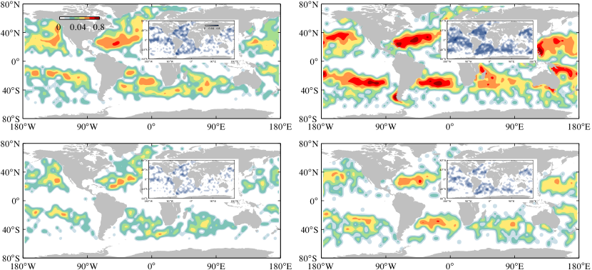
Figure 1: Expressed as number per degree squared, density of drogued (left) and undrogued (right) drifters from the NOAA Global Drifter Program over 1979–2015 after at least 1 (top) or exactly 1.5 (bottom) yr past the time at deployment for drogued drifters or the location where a drifter loses the drogue (insets).

The tendency of undrogued drifters to accumulate in the North and South Atlantic gyres is particularly robust as it is not influenced by the disparity in the amounts (1621 vs 2895) and mean lifetimes (1.5 vs 2 yr) of the drogued and undrogued drifters used in the construction of the top panels of Fig. 1. This follows from the inspection of the bottom panels, which show the same as in the top panels but restricted to equal number of drifters (826) and length of the trajectory records (1.5 yr).

The reported accumulation tendency had been inferred earlier, but for both undrogued and drogued drifters and from the topology of ensemble-mean streamlines constructed using drifter velocities (Maximenko et al., 2012). These authors found their result unexpected given the different water-following characteristics of drogued and undrogued drifters (Niiler and Paduan, 1995). The discrepancy with our finding may be attributed to errors in the drogue presence verification, which were discovered at the time of that publication and corrected in Lumpkin et al. (2012).

The accumulation inferred in Maximenko et al. (2012) was explained as a consequence of Ekman transport using steady flow arguments on fluid particle motion. In the next section we show that inertial effects provide an explanation for the accumulation when spherical float motion opposed by unsteady water and air flow drag is considered.

3 Simulated accumulation

Consider a small spherical particle of radius $a$ and density $\rho_{\mathrm{p}}\leq\rho$, where $\rho$ and $\rho_{\mathrm{a}}$ are the water and air densities. The fraction of water volume displaced by the particle is $\delta^{-1}$, where

$$\delta:=\frac{\rho}{\rho_{\mathrm{p}}}.$$ (1)

Posing the exact motion equation for a buoyant finite-size particle immersed in a fluid in motion is a challenging task (Cartwright et al., 2010), which was solved to a very good approximation by Maxey and Riley (1983). As a first step toward posing that for a particle at the air–sea interface, the more complicated case of interest here, we proceed heuristically by modeling the particle piece immersed in the water (air) as a sphere of the fractional volume that is immersed in the water (air), and assuming that it evolves according to the Maxey–Riley set. Adding the forces acting on each of the spheres as if they were decoupled from one another, we obtain (cf. Supporting Information, Appendix A):

$$\ddot{x}+f\dot{x}^{\perp}=\mathrm{D}_{t}v+fv^{\perp}-\frac{2\left(\gamma+\sqrt[3]{\delta-1}\right)}{3\gamma\sqrt[3]{\delta}\tau}\left(\dot{x}-u\right),$$ (2)

where

$$u:=\frac{\gamma v+\sqrt[3]{\delta-1}v_{\mathrm{a}}}{\gamma+\sqrt[3]{\delta-1}}.$$ (3)

Here $x$ denotes position on the horizontal plane; $v$ and $v_{\mathrm{a}}$ are water and air velocities; $\mathrm{D}_{t}:=\partial_{t}+v\cdot\nabla$; $f$ is the Coriolis parameter; and

$$\tau:=\frac{2a^{2}}{9\nu\delta},\quad\gamma:=\frac{\nu\rho}{\nu_{\mathrm{a}}\rho_{\mathrm{a}}},$$ (4)

where $\nu$ and $\nu_{\mathrm{a}}$ are water and air dynamic viscosities. The left-hand-side of (2) is the absolute acceleration of the particle. The first and second terms on the right-hand-side are flow and drag forces mediated by added mass effects, respectively, which water and air exert on the particle.

The Maxey–Riley equation (2) constitutes a nonautonomous four-dimensional dynamical system for the particle position and velocity, $v_{\mathrm{p}}=\dot{x}$. To integrate it one must specify both initial particle position and velocity, which is not known in general. In addition, long reversed-time integrations of (2), which are useful for instance in pollution source detection, are not feasible because the term $u/\tau$ tends to cause numerical instability as it has been noted earlier for the standard Maxey–Riley equation (Haller and Sapsis, 2008).

However, for a sufficiently small particle ($\tau\to 0$) the Maxey–Riley equation (2) reduces to (cf. Supporting Information, Appendix B)

$$\dot{x}=v_{\mathrm{p}}=u+\frac{3\gamma\sqrt[3]{\delta}\tau}{2\left(\gamma+\sqrt[3]{\delta-1}\right)}\left(\mathrm{D}_{t}v+fv^{\perp}-fu^{\perp}\right).$$ (5)

This equation, which will be referred to as an inertial equation, constitutes a two-dimensional system in the position, and thus can be integrated without knowledge of the initial velocity. Also, it is not subjected to numerical instability in long backward-time integration. Up to an $O(\tau^{2})$ error, the particle velocity is equal to a weighted average of the water and air velocities ($u$) plus a term proportional to the water absolute and Coriolis (due to $u$) accelerations times $\tau$, the particle timescale.

To carry out the integration of (5) realizations of $v$ and $v_{\mathrm{a}}$ near the ocean–atmosphere interface are needed. Here we have chosen to consider $v$ as given by surface ocean velocity from the Global $1/12^{\circ}$ HYCOM (HYbrid-Coordinate Ocean Model) $+$ NCODA (Navy Coupled Ocean Data Assimilation) Ocean Reanalysis (GLBu0.08/expt_19.0) (Cummings and Smedstad, 2013). In turn, we take $v_{\mathrm{a}}$ as the wind velocity from the National Centers for Environmental Prediction (NCEP) Climate Forecast System Reanalysis (CFSR), which is employed to construct the wind stress applied on the model.

Also needed for the integration of (5) are estimates of parameters $\gamma$, $\delta$, and $\tau$. For typical water and air density and viscosity values, $\gamma\approx 60$. From the configuration of the undrogued drifters we infer $\delta=2$ (about half of the spherical float is submerged when the drogue is not present) and further estimate $\tau\approx 0.05$ d (the mean radius of the float is about 17.5 cm). Note that $\tau$ is small compared to relevant timescales such as the turnover time of a mesoscale eddy (a few days) or a subtropical gyre (a few years) (Vallis, 2006).

For the above velocity realizations and parameter choices we begin by integrating the inertial equation (5) using a Runge–Kutta method from a uniform distribution of particles. For comparison we also integrate $\dot{x}=v$ from the same positions. In both cases integrations are initialized along three simulation years (2005–2007). Starting on the drifter deployment positions or where the drifters lose their drogues on the corresponding dates is not possible because model output is not available over the entire drifter trajectory records. The proposed ensemble integrations facilitate intercomparisons and also guarantee robustness of the results. The integrations are carried over a period of 4 yr, which is sufficiently long to reveal accumulation (undrogued drifters show clear signs of accumulation after about 1.5 yr). For convenience we restrict the analysis to the North Atlantic; similar results are attained in the other basins.

The density (normalized by initial density) of inertial particles, i.e., controlled by (5), after 1.5 (Fig. 2, top-left panel) and 4 (Fig. 2, middle-left panel) yr is high in the center of the subtropical gyre as is that of undrogued drifters . Note also (in the insets) that particles controlled by the Maxey–Riley equation (2) (circles) take similar final distributions as inertial particles (dots). This confirms the validity of (5), which attracts solutions of (2).

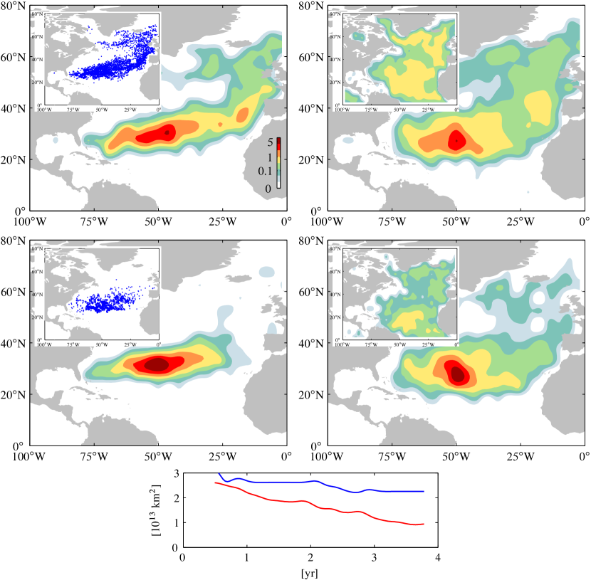
Figure 2: Density of particles after 1.5 (top) and 4 (middle) yr of integration of the inertial equation (5) (left) and of advection by water velocity (right) normalized by density in the initially uniform distribution of particles. Insets in the left show final positions of inertial particles (dots) and particles obeying the full Maxey–Riley equation (2) (circles). Insets in the right show normalized density for particles advected by velocity derived geostrophically from sea-surface height. In the bottom panel, as function of time, area of the region where normalized particle density is higher than 1% for inertial (red) and water (blue) particles. Water velocity is given by surface ocean velocity from the 1/12^∘ Global HYCOM$+$NCOM Ocean Reanalysis, from which sea-surface height is also taken. The air velocity corresponds to the wind velocity from the NCEP/CFSR reanalysis used to construct the wind stress that forces the model.

By contrast, after 1.5 yr water particles, i.e., controlled by $\dot{x}=v$, take a more homogeneous distribution (Fig. 2, top-right panel), which is in better agreement with the distribution taken by drogued drifters . Accumulation in this case, most evident after 4 yr (Fig. 2, middle-right panel), can be attributed to Ekman transport by comparing these distributions with the much more homogeneous distributions attained by the particles when $v$ is taken as geostrophic (i.e., divergenceless) velocity inferred from the model sea surface height (SSH) field (insets).

Accumulation due to Ekman transport is a slow process. This is evident from the inspection of the bottom panel of Fig. 2, which shows that the region where normalized particle density is higher than 1% decays nearly two times faster for inertial particles than for water particles. While there are not enough sufficiently long drogued drifter trajectories to verify this behavior, application of a probabilistic approach similar to that used earlier (Maximenko et al., 2012; van Sebille et al., 2012) on such drifters suggests it .

The behavior of the inertial particles just described can be anticipated by considering an idealized model of the large-scale circulation in the North Atlantic. In the simplest such models, due to Stommel (1966), the slow steady flow is divergenceless ($\nabla\cdot v=0$) and has an anticyclonic basin-wide gyre, driven by strong steady westerlies and trade winds, so $\nabla\cdot v_{\mathrm{a}}=0$. Under such conditions,

$$\nabla\cdot v_{\mathrm{p}}\approx\frac{3\gamma\sqrt[3]{\delta}\tau}{2\left(\gamma+\sqrt[3]{\delta-1}\right)^{2}}\sqrt[3]{\delta-1}f\omega_{\mathrm{a}},$$ (6)

where $\omega_{\mathrm{a}}:=-\nabla\cdot v_{\mathrm{a}}^{\perp}$ is the air vorticity. Because $f\omega_{\mathrm{a}}<0$, (6) is negative, which promotes accumulation of inertial particles in the center of the gyre. In other words, inertia-induced accumulation occurs on a faster timescale than Ekam convergence, which is a higher order (in the Rossby number) effect in Stommel’s model.

A pertinent question is if undrogued drifter accumulation may be inferred by simply considering $\dot{x}=v+\alpha\,v_{\mathrm{a}}$ with $\alpha>0$ small, an ad-hoc model widely used to simulate windage effects on floating matter in the ocean (Duhec et al., 2015). Use of $\alpha=0.01$ suggests that it may indeed be possible after 1.5 yr of evolution (Fig. 3, left panel), but use of a slightly larger value within the commonly used range such as $\alpha=0.05$ reveals leakage of particles in the southwest direction (Fig. 3, middle panel). This emphasizes the importance of finite-size effects. More specifically, for undrogued drifter parameters $u\approx 0.99\,v+0.02\,v_{\mathrm{a}}$ in (3), which incidentally is close to the ad-hoc models just considered. This is the first term in the inertial equation (5). Finite-size effects are accounted for in the second term.

Figure 3: As in in the top panels of Fig. 2, but for particles advected for 1.5 yr using model velocity with 1% (right) and 5% (middle) windage added, and obeying the inertial equation (5) with the water velocity derived geostrophically from the model sea-surface height output (right).

Another relevant question is if accumulation is revealed when SSH-derived instead of full $v$ is used in the inertial equation (5). The relevance of this question stems from the wide use of satellite altimetry measurements of SSH in diagnosing surface ocean currents (Fu et al., 2010). The answer to the question is partially affirmative as the final particle position distribution reveals (Fig. 3, right panel). A similar result is attained if altimetric SSH is employed.

4 Concluding remarks

We conclude that undrogued drifters are quite strongly influenced by inertial effects. Drogued drifters, by contrast, appear to more closely follow the water motion. Ekman transport contributes to accumulate water, but this acts on a longer time scale than inertial effects. We infer, then, that marine plastic debris, which accumulate in the same places as undrogued drifters, and flotsam in general must be affected by inertial effects in a similar manner as undrogued drifters.

We close by noting that shipwreck and airplane debris tracking, pollution source identification, and search and rescue operations at sea are among the many practical applications that may benefit from the use of the inertial equation derived here. Whether inaccuracies resulting from our heuristic derivation of this equation and omission of a number of potentially important processes (Stokes drift, infragravity waves, subgrid motions, etc.) or the quality of the velocity realizations will constrain more its success in such applications is a subject of ongoing research.

Appendix A The Maxey–Riley equation

The exact motion of inertial particles in the flow of a fluid is controlled by the Navier–Stokes equation with moving boundaries as such particles are extended objects in the fluid with their own boundaries [Cartwright et al., 2010]. This approach results in complicated partial differential equations which are very difficult—if not impossible—to solve and interpret. However, a good approximation to the motion of a small spherical particle, formulated in terms of an ordinary differential equation (ODE), is provided by the Maxey–Riley equation [Maxey and Riley, 1983]. Assuming that the time it takes such a particle to revisit a given region is long, so the Basset history term can be ignored, such equation is a classical mechanics Newton equation of the form:

$$m_{\mathrm{p}}a_{\mathrm{p}}=\mathcal{F}_{\mathrm{FF}}+\mathcal{F}_{\mathrm{AM}}+\mathcal{F}_{\mathrm{SD}}.$$ (7)

On the left-hand-side of (7), $m_{\mathrm{p}}=\frac{4}{3}\pi a^{3}\rho_{\mathrm{p}}$ is the mass of the particle and $a_{\mathrm{p}}$ is its acceleration. In the case of interest where the fluid is geophysical such acceleration is the absolute acceleration, which is given by [Provenzale, 1999; Beron-Vera et al., 2015]:

$$a_{\mathrm{p}}=\ddot{x}+f\dot{x}^{\perp},$$ (8)

where $x$ denotes position on a plane tangent to the Earth, which rotates with angular velocity $\frac{1}{2}f$. (The centrifugal acceleration was also included in Provenzale [1999] , but this is actually balanced out by the gravitational acceleration on the plane. Also, geometric terms due to the Earth sphericity are omitted for simplicity. While trajectory details depend on such terms [Ripa, 1997], they do not affect the results of the paper. For completeness, the full spherical forms of Maxey–Riley and inertial equations are given in Appendix C.

On the right-hand-side of (7), $\mathcal{F}_{\mathrm{SD}}$ denotes the drag force. Assuming that the flow is laminar, this force is described by the Stokes law. Deriving an exact expression for a spherical drifter at the water–air interface will require one to write the projected area of the submerged (surfaced) part in terms of the water-to-particle density ratio, $\delta$, whose inverse determines the submerged water volume, but this does not seem feasible or simple at least. So we approach the problem heuristically by modelling the submerged portion of the drifter as a sphere of the fractional volume that is submerged and the surfaced piece as another sphere of the fractional volume that is surfaced. The radius of the sphere immersed in the water is $\sqrt[3]{\delta^{-1}}\,a$, while that of the sphere immersed in the air is $\sqrt[3]{1-\delta^{-1}}\,a$. Neglecting Faxen corrections, which is reasonable for a small particle, we write the drag force as a superposition of the drag forces acting on the spheres as if they were well separated from one another:

$$\mathcal{F}_{\mathrm{SD}}=\sqrt[3]{\delta^{-1}}6\pi a\nu\rho(v-\dot{x})+\sqrt[3]{1-\delta^{-1}}6\pi a\nu_{\mathrm{a}}\rho_{\mathrm{a}}(v_{\mathrm{a}}-\dot{x}).$$ (9)

Force $\mathcal{F}_{\mathrm{AM}}$ describes added mass effects, which in the present case are due to the displacement of both water and air as the particle moves. To write an exact expression for this force one should know the potential flow around a sphere at the interface between two fluids in motion, which is not known in closed form. Thus we proceed as above and write it as a superposition of the added masses by the two spheres. This leads to the following explicit form:

$$\mathcal{F}_{\mathrm{AM}}={} -\frac{1}{2}\delta^{-1}m\left(\ddot{x}+f\dot{x}^{\perp}-\mathrm{D}_{t}v-fv^{\perp}\right)$$

$$-\frac{1}{2}(1-\delta^{-1})m_{\mathrm{a}}\left(\ddot{x}+f\dot{x}^{\perp}-\mathrm{D}_{\mathrm{a}t}v_{\mathrm{a}}-fv_{\mathrm{a}}^{\perp}\right),$$ (10)

where $\mathrm{D}_{\mathrm{a}t}:=\partial_{t}+v_{\mathrm{a}}\cdot\nabla$, $m=\frac{4}{3}\pi a^{3}\rho$, and $m_{\mathrm{a}}=\frac{4}{3}\pi a^{3}\rho_{\mathrm{a}}$. Finally, term $\mathcal{F}_{\mathrm{FF}}$ is the flow force, here exerted by both water and air on the particle. Proceeding as before, this reads:

$$\mathcal{F}_{\mathrm{FF}}=\delta^{-1}m\left(\mathrm{D}_{t}v+fv^{\perp}\right)+(1-\delta^{-1})m_{\mathrm{a}}\left(\mathrm{D}_{\mathrm{a}t}v_{\mathrm{a}}+fv_{\mathrm{a}}^{\perp}\right).$$ (11)

With the above explicit forms of each of the terms in (7), and taking into account that $\rho\gg\rho_{\mathrm{a}}$, the Maxey–Riley equation (2) follows.

Appendix B The inertial equation

The second-order ODE (2) is equivalent to the following first-order ODE set:

$$\dot{x}=v_{\mathrm{p}},\quad\dot{v}_{\mathrm{p}}=\mathrm{D}_{t}v+f(v-v_{\mathrm{p}})^{\perp}-\frac{2\left(\gamma+\sqrt[3]{\delta-1}\right)}{3\gamma\sqrt[3]{\delta}\tau}(v_{\mathrm{p}}-u).$$ (12)

When $\tau=0$, $v_{\mathrm{p}}=u$, which suggests the asymptotic series expansion $v_{\mathrm{p}}=u+u_{1}+u_{2}+\cdots$ where $u_{n}=O(\tau^{n})$. Plugging this series into the right-hand-side equation of system (12) and equating $O(\tau)$ terms, it follows that

$$u_{1}=\frac{3\gamma\sqrt[3]{\delta}}{2\left(\gamma+\sqrt[3]{\delta-1}\right)}\left(\mathrm{D}_{t}v+fv^{\perp}-fu^{\perp}\right).$$ (13)

Inserting this expression in the left-hand-side equation of system (12), the inertial equation (5), valid up to an $O(\tau^{2})$ error, follows. For the interpretation of (5) as a slow manifold of (12), cf. Haller and Sapsis [2008].

A few remarks relating to limiting behavior of the inertial equation (5) are in order. A sizeless ($\tau=0$) neutrally-buoyant ($\delta=1$) particle behaves as expected as a fluid particle because (2) reduces in this limit to

$$\dot{x}=v_{\mathrm{p}}=v.$$ (14)

Sizeless ($\tau=0$) but buoyant ($\delta>1$) particles obey

$$\dot{x}=v_{\mathrm{p}}=u,$$ (15)

where $u$ a weighted average of the air and water velocities. When a particle is completely exposed to the air above the water ($\delta\to\infty$), the inertial equation (5) reduces to

$$\dot{x}=v_{\mathrm{p}}=v_{\mathrm{a}},$$ (16)

i.e., its motion is completely driven by the air velocity as expected. A neutrally buoyant particle ($\delta=1$) obeys

$$\dot{x}=v_{\mathrm{p}}=v+\frac{3}{2}\tau\mathrm{D}_{t}v,$$ (17)

i.e., its behavior differs from that of a fluid particle unless $\mathrm{D}_{t}v$ can be neglected in front of $v$ (the water flow is nearly geostrophic). If the air above the water is replaced by vacuum ($\gamma\to\infty$), in which case particle motion is opposed by water drag exclusively,

$$\dot{x}=v_{\mathrm{p}}=v+\frac{3}{2}\sqrt[3]{\delta}\tau\mathrm{D}_{t}v.$$ (18)

When the air is quiescent ($v_{\mathrm{a}}=0$),

$$\dot{x}={} v_{\mathrm{p}}=\frac{\gamma v}{\gamma+\sqrt[3]{\delta-1}}$$

$$+\frac{3\gamma\sqrt[3]{\delta}\tau}{2\left(\gamma+\sqrt[3]{\delta-1}\right)}\left(\mathrm{D}_{t}v+\frac{\sqrt[3]{\delta-1}}{\gamma+\sqrt[3]{\delta-1}}fv^{\perp}\right).$$ (19)

This is different than the vacuum case as particle motion is opposed by both water and air drags.

Finally, the inertial equation derived by Beron-Vera et al. [2015] does not follow as a limiting case of the inertial equation derived here as that one implicitly assumes that the particle is completely immersed in the water (density stratification must be allowed in order for nearly horizontal motion to be possible in such a case). However, the attracting (repelling) role of cyclonic (anticyclonic) coherent Lagrangian eddies [Haller and Beron-Vera, 2013; 2014] which requires the water flow to be nearly geostrophic, predicted for floating objects is still realized for sufficiently calm air. In a such case $\mathrm{D}_{t}v$ can be neglected in right-hand-side of (19), so

$$\nabla\cdot v_{\mathrm{p}}=-\frac{3\gamma\sqrt[3]{\delta(\delta-1)}\tau}{2\left(\gamma+\sqrt[3]{\delta-1}\right)^{2}}f\omega,$$ (20)

where $\omega=-\nabla\cdot v^{\perp}$ is the water vorticity. Note that the sign of (20) is determined by $f\omega$, and thus the conclusions that follow from (11) in Beron-Vera et al. [2015] for light particles (i.e., with $\delta>1$) follow from (20) as well.

Appendix C The equations in full spherical geometry

Let $\lambda$ ($\vartheta$) be longitude (latitude) and $R$ the mean Earth radius. Then the Maxey–Riley equation reads:

$$\dot{\lambda}={} R^{-1}\sec\vartheta\,v_{\mathrm{p}}^{\lambda},$$ (21)

$$\dot{\vartheta}={} R^{-1}v_{\mathrm{p}}^{\vartheta}$$ (22)

$$\dot{v}_{\mathrm{p}}^{\lambda}={} \mathrm{D}_{t}v^{\lambda}+f(v_{\mathrm{p}}^{\vartheta}-v^{\vartheta})+\psi(v_{\mathrm{p}}^{\lambda}v_{\mathrm{p}}^{\vartheta}-v^{\lambda}v^{\vartheta})$$

$$-\frac{2(\gamma+\sqrt[3]{\delta-1})}{3\gamma\sqrt[3]{\delta}\tau}\big{(}v_{\mathrm{p}}^{\lambda}-u^{\lambda}\big{)},$$ (23)

$$\dot{v}_{\mathrm{p}}^{\vartheta}={} \mathrm{D}_{t}v^{\vartheta}+f(v^{\lambda}-v_{\mathrm{p}}^{\lambda})+\psi(v^{\lambda}v^{\lambda}-v_{\mathrm{p}}^{\lambda}v_{\mathrm{p}}^{\lambda})$$

$$-\frac{2(\gamma+\sqrt[3]{\delta-1})}{3\gamma\sqrt[3]{\delta}\tau}\big{(}v_{\mathrm{p}}^{\vartheta}-u^{\vartheta}\big{)},$$ (24)

where $\psi:=R^{-1}\tan\vartheta$ and $\mathrm{D}_{t}=\partial_{t}+R^{-1}\sec\vartheta\,v^{\lambda}\partial_{\lambda}+R^{-1}v^{\vartheta}\partial_{\vartheta}$.

The inertial equation, in turn, takes the form:

$$\dot{\lambda}={} R^{-1}\sec\vartheta\bigg{(}u^{\lambda}+\frac{3\gamma\sqrt[3]{\delta}\tau}{2(\gamma+\sqrt[3]{\delta-1})}\Big{(}\mathrm{D}_{t}v^{\lambda}$$

$$+f(u^{\vartheta}-v^{\vartheta})+\psi(u^{\lambda}u^{\vartheta}-v^{\lambda}v^{\vartheta})\Big{)}\bigg{)},$$ (25)

$$\dot{\vartheta}={} R^{-1}\bigg{(}u^{\vartheta}+\frac{3\gamma\sqrt[3]{\delta}\tau}{2(\gamma+\sqrt[3]{\delta-1})}\big{(}\mathrm{D}_{t}v^{\vartheta}$$

$$+f(v^{\lambda}-u^{\lambda})+\psi(v^{\lambda}v^{\lambda}-u^{\lambda}u^{\vartheta})\Big{)}\bigg{)}.$$ (26)

References

- Beron-Vera et al. (2015) Beron-Vera, F. J., M. J. Olascoaga, G. Haller, M. Farazmand, J. Triñanes, and Y. Wang (2015), Dissipative inertial transport patterns near coherent Lagrangian eddies in the ocean, Chaos, 25, 087,412, 10.1063/1.4928693.
- Cartwright et al. (2010) Cartwright, J. H. E., U. Feudel, G. Károlyi, A. de Moura, O. Piro, and T. Tél (2010), Dynamics of finite-size particles in chaotic fluid flows, in Nonlinear Dynamics and Chaos: Advances and Perspectives, edited by M. Thiel et al., pp. 51–87, Springer-Verlag Berlin Heidelberg.
- Cozar et al. (2014) Cozar, A., et al. (2014), Plastic debris in the open ocean, Proc. Nat. Acad. Sci. USA, 111(28), 10,239–10,244, 10.1073/pnas.1314705111.
- Cummings and Smedstad (2013) Cummings, J. A., and O. M. Smedstad (2013), Variational data analysis for the global ocean, in Data Assimilation for Atmospheric, Oceanic and Hydrologic Applications, vol. 2, edited by S. K. Park and L. Xu, chap. 13, Springer-Verlag Berlin Heidelberg, 10.1007/978-3-642-35088-7-13.
- Duhec et al. (2015) Duhec, A. V., R. F. Jeanne, N. Maximenko, and J. Hafner (2015), Composition and potential origin of marine debris stranded in the Western Indian Ocean on remote Alphonse Island, Seychelles, Mar. Poll. Bull., 96(1–2), 76–86, 10.1016/j.marpolbul.2015.05.042.
- Fu et al. (2010) Fu, L. L., D. B. Chelton, P.-Y. Le Traon, and R. Morrow (2010), Eddy dynamics from satellite altimetry, Oceanography, 23, 14–25.
- Haller and Beron-Vera (2013) Haller, G., and F. J. Beron-Vera (2013), Coherent Lagrangian vortices: The black holes of turbulence, J. Fluid Mech., 731, R4, 10.1017/jfm.2013.391.
- Haller and Beron-Vera (2014) Haller, G., and F. J. Beron-Vera (2014), Addendum to ‘Coherent Lagrangian vortices: The black holes of turbulence’, J. Fluid Mech., 755, R3.
- Haller and Sapsis (2008) Haller, G., and T. Sapsis (2008), Where do inertial particles go in fluid flows?, Physica D, 237, 573–583.
- Lumpkin and Pazos (2007) Lumpkin, R., and M. Pazos (2007), Measuring surface currents sith Surface Velocity Program driftres: the instrument, its data and some recent results, in Lagrangian Analysis and Prediction of Coastal and Ocean Dynamics, edited by A. Griffa, A. D. Kirwan, A. Mariano, T. Özgökmen, and T. Rossby, chap. 2, pp. 39–67, Cambridge University Press.
- Lumpkin et al. (2012) Lumpkin, R., S. A. Grodsky, L. Centurioni, M.-H. Rio, J. A. Carton, and D. Lee (2012), Removing spurious low-frequency variability in drifter velocities, J. Atm. Oce. Tech., 30, 353–360, 10.1175/JTECH-D-12-00139.1.
- Maxey and Riley (1983) Maxey, M. R., and J. J. Riley (1983), Equation of motion for a small rigid sphere in a nonuniform flow, Phys. Fluids, 26, 883.
- Maximenko et al. (2012) Maximenko, A. N., J. Hafner, and P. Niiler (2012), Pathways of marine debris derived from trajectories of Lagrangian drifters, Mar. Pollut. Bull., 65, 51–62.
- Niiler and Paduan (1995) Niiler, P. P., and J. D. Paduan (1995), Wind-driven Motions in the northeastern Pacific as measured by Lagrangian drifters, J. Phys. Oceanogr., 25, 2819–2830.
- Provenzale (1999) Provenzale, A. (1999), Transport by coherent barotropic vortices, Annu. Rev. Fluid Mech., 31, 55–93.
- Ripa (1997) Ripa, P. (1997), “Inertial” oscillations and the -plane approximation(s), J. Phys. Oceanogr., 27, 633–647.
- Stommel (1966) Stommel, H. (1966), The Gulf Stream, 2nd ed., University of California.
- Sybrandy and Niiler (1991) Sybrandy, A. L., and P. P. Niiler (1991), WOCE/TOGA Lagrangian drifter contruction manual, Tech. Rep. SIO Reference 91/6, Scripps Institution of Oceanography, La Jolla, California.
- Tanga and Provenzale (1994) Tanga, P., and A. Provenzale (1994), Dynamics of advected tracers with varying buoyancy, Physica D, 76, 202–215.
- Vallis (2006) Vallis, G. K. (2006), Atmospheric and oceanic fluid dynamics, Cambridge University.
- van Sebille et al. (2012) van Sebille, E., E. H. England, and G. Froyland (2012), Origin, dynamics and evolution of ocean garbage patches from observed surface drifters, Environ. Res. Lett., 7, 044,040.